Symmetrical Learning and Transferring: Efficient Knowledge Distillation for Remote Sensing Image Classification

Abstract

Knowledge distillation (KD) is crucial for remote sensing image (RSI) classification, particularly as the operating environment in remote sensing is often constrained by hardware limitations. However, prior research has not fully addressed the challenge of leveraging KD to develop lightweight, high-accuracy models for RSI classification. A key issue is the sparse distribution of training data, which often results in asymmetry within the data. This asymmetry impedes the transfer of prior knowledge during the distillation process, diminishing the overall efficacy of KD techniques. To overcome this challenge, we propose a novel, symmetry-enhanced approach that augments the logit-based KD process, improving its effectiveness and efficiency for RSI classification. Our method is distinguished by three core innovations: a symmetrically generative algorithm to enhance the symmetry of the training data, an efficient algorithm for constructing a robust teacher ensemble model, and a quantitative technique for feature alignment. Rigorous evaluations on three benchmark datasets demonstrate that our method outperforms 14 existing KD-based approaches and 30 other state-of-the-art methods. Specifically, the student model trained with our approach achieves accuracy improvements of up to 22.5% while reducing the model size and inference time by as much as 96% and 88%, respectively. In conclusion, this research makes a significant contribution to RSI classification by introducing an efficient and effective data symmetry-driven method to enhance the knowledge transferring efficiency of the logit-based KD process.

1. Introduction

Remote sensing images (RSIs) are observational data captured from airborne platforms and serve as powerful tools for monitoring Earth systems [1]. As Earth observation significantly increases, computer algorithms have progressively supplanted human involvement in various RSI recognition tasks for automation and intelligence [2,3,4]. Among these algorithms, classification plays a pivotal role, as enhancements in classification performance often lead to improved outcomes for related tasks, such as object detection and segmentation [5]. The advent of deep learning has further propelled RSI classification, with convolutional neural networks (CNNs) and vision Transformers (ViTs) emerging as the primary models due to their capabilities in automatic feature extraction and superior accuracy [6,7,8].

Deep learning models retain prior knowledge within large-scale datasets through pre-training, thereby excelling in downstream tasks via transfer learning. However, the remote sensing domain is often task-specific, resulting in a scarcity of large-scale datasets [9,10,11]. Consequently, state-of-the-art methods commonly utilize models pre-trained on ImageNet-1K, a large-scale dataset of natural images, for RSI classification. Furthermore, although ViTs currently achieve higher accuracy with high-resolution samples—owing to their ability to model long-range dependencies—CNNs continue to outperform ViTs when RSI resolution decreases [12,13,14,15,16]. This performance disparity is attributable to the diminished capability of ViTs to capture feature dependencies in low-quality images. Moreover, the larger parameter counts and slower inference speeds associated with ViTs further underscore the continued importance of CNNs, especially in applications that require rapid inference [17,18,19,20].

Recent advances have focused on structurally modifying classic CNN and ViT architectures to boost accuracy [21,22,23]. These designs commonly introduce additional modules or merge multiple models, leading to increased parameters and enlarged model sizes. As a result, inference speeds decline while accuracy gains remain marginal relative to the original networks [24]. Moreover, performance often degrades sharply under limited training data—a pervasive issue in remote sensing [25,26]. Given the stringent requirements for compact models, fast inference, and robustness in many RSI applications, these constraints hinder the general applicability of existing methods [27,28,29].

Pruning, a straightforward model compression technique, enhances inference speed at the expense of accuracy [30,31]. On the other hand, knowledge distillation (KD), a method that employs a high-accuracy, heavyweight model (teacher) to guide a lightweight model (student), shows great promise in creating compact classifiers with superior accuracy [32,33,34]. KD techniques include feature-based and logit-based frameworks. Feature-based methods typically incorporate additional structures to align the intermediate-layer features of the student and teacher models [35]. Conversely, logit-based methods transfer knowledge exclusively through the prediction logits of the teacher and student models [36,37]. Therefore, logit-based KD can yield more compact classifiers with a simple pipeline as it eliminates the need for structural modifications and additional parameters in the models.

Currently, research on the application of KD for RSI classification is notably limited. Specifically, existing studies often face two primary shortcomings: the teacher models lack competitive accuracy [38,39,40,41], and the KD phase is inefficient in knowledge transfer. These issues frequently result in a substantial accuracy gap between the teacher and student models [42,43,44,45], with the latter often exhibiting subpar performance. Consequently, existing studies have yet to demonstrate that KD techniques can effectively and efficiently produce lightweight classifiers with superior accuracy [46,47,48,49,50,51]. We posit that these challenges stem from specific factors.

Pre-trained models on ImageNet-1K contain rich prior knowledge that facilitates the classification of new, unseen imagery. Moreover, regularization techniques further enhance model performance by promoting the identification of generalizable features. These techniques improve the model’s capacity to recognize key attributes, including symmetrical patterns, across a wide range of examples. However, when applied to RSIs, the effectiveness of these regularization methods may be compromised due to inherent asymmetries in the data, such as variations in object size, complex backgrounds, and domain-specific conditions.

As illustrated in Figure 1, natural images typically exhibit a clear separation between objects and backgrounds, with the objects occupying a prominent portion of the image. This clear distinction allows regularization techniques like MixUp or CutMix to operate effectively, as swapping background patches (marked by red rectangles) between images does not significantly affect the object’s symmetrical characteristics or category definition. In contrast, RSIs often contain smaller objects (marked by red rectangles) situated against more intricate and heterogeneous backgrounds. When such techniques are applied to RSIs, the inherent asymmetry of the data means that swapping patches can disrupt not only the spatial layout but also the perceived symmetry of the object. For example, exchanging patches between images of a baseball field and a basketball court may alter not only the background but also the object structure and symmetry, leading to potential misclassification. Thus, the failure to properly account for symmetry during data augmentation (DA) could severely hinder the model’s ability to generalize across different orientations, scales, and object configurations in RSIs.

The unique imaging conditions of RSIs further exacerbate these challenges. Figure 2 (see below) shows that variations in sunlight intensity—due to time of day or atmospheric conditions—significantly influence the quality and symmetry of RSIs. At optimal illumination (samples A and B in Figure 2), RSIs exhibit high-quality images with clear, recognizable objects. However, subtle variations in the Sun’s elevation angles can result in asymmetric lighting, introducing larger inter-class dissimilarities between otherwise similar scenes. In these cases, the objects within the image may appear skewed or distorted, further complicating the model’s ability to learn symmetrical features. When sunlight dims or the focus is off (samples C, D, and E), the contrast ratio decreases, and the images become blurred, introducing additional asymmetries that pose challenges for object recognition and classification. The presence of such asymmetric lighting and focus distortions requires models to be robust to these variations in symmetry, which traditional regularization techniques do not sufficiently address.

Moreover, due to the limited availability of RSI data, training models on a small subset of samples often introduces significant data distribution shifts. These shifts are especially problematic when low-quality samples, which tend to exhibit asymmetry in lighting, focus, or contrast, are overrepresented. Traditional DA techniques, which simulate low-quality samples, typically apply binary transformations that either add or exclude certain features, leading to an artificially skewed distribution of sample quality. These methods fail to account for the underlying asymmetry of the RSI dataset as they do not preserve the inherent symmetry of high-quality samples. Consequently, these qualitative DA strategies result in biased training subsets that exacerbate the existing data imbalances, hindering the model’s ability to capture symmetrical features across all conditions.

In deep learning, models function as complex mappings, where models transform input samples (denoted as $x$) into predictions ($y$). The KD approach aims to minimize the prediction biases between a teacher model ($f_t$) and a student model ($f_s$) by approximating the teacher’s output. It becomes particularly challenging when training on mini-batches, as hardware limitations prevent the use of the entire dataset in one iteration. This issue introduces variance within mini-batches which, if not properly handled, can significantly disrupt the KD process.

As shown in Figure 3 (see below), when the variance ($D\left(x\right)$) within the mini-batches is small (Section A), the student model can more easily converge to the teacher’s predictions. However, when the variance is large (Section B), the biases between the teacher and student models become more pronounced, as the student must frequently adjust to the asymmetries in the data. This leads to larger accuracy gaps and difficulty in capturing symmetrical relationships across the dataset. Given that RSIs often exhibit such asymmetries—due to lighting, sensor issues, and complex backgrounds—this problem is exacerbated.

The right side of Figure 3 demonstrates how DA techniques can help mitigate variance by generating augmented data points (red dots) that guide the student model toward reducing biases relative to the teacher. However, excessive use of DA can introduce a large number of synthetic samples with varying levels of asymmetry (black dots). These unknown samples with large variances may lead to increased biases between the teacher and student models. In this context, traditional DA strategies fail to preserve the symmetry of the dataset and thus undermine the KD process. A more effective approach would involve symmetry-aware DA techniques that are tailored to preserve the object symmetry across transformations, ensuring that the augmented data maintains the structural consistency of objects within RSIs.

In this study, we propose a novel and entirely data-driven approach that addresses the challenges identified in the literature while significantly enhancing the effectiveness and efficiency of the knowledge distillation process for RSI classification. Our method distinguishes itself in four key areas.

First, we propose a symmetric generative algorithm to replace conventional augmentation and regularization, ensuring augmented RSI samples preserve their intrinsic object symmetry and thus reducing data imbalance. Second, we introduce a simple yet effective method for assembling an ensemble of lightweight CNNs, leveraging diversity among individual models to yield a more capable teacher network. Third, we develop quantitative feature alignment, a novel mechanism that aligns the distribution of augmented samples in the knowledge distillation phase with those used to train the teacher—preserving feature symmetry and inter-sample relationships within mini-batches. Finally, we integrate these components into a plug-and-play symmetrical learning and transferring (SLT) module, enabling seamless adoption and deployment.

We evaluate our method on three benchmark RSI classification datasets. Experimental results demonstrate that our student model achieves superior accuracy while substantially narrowing the performance gap with its teacher model. The key contributions of this study are as follows:

(1)

Symmetry-aware KD: We propose the SLT strategy, which addresses the challenge of preserving symmetry in RSI samples during the KD process. By ensuring that augmented data maintains spatial and feature symmetry, our method enhances the alignment between the teacher and student models, leading to more accurate knowledge transfer and reduced accuracy discrepancies.

(2)

Improved KD-based approach for RSI classification: Our approach introduces a symmetry-aware KD method that outperforms previous techniques with accuracy improvements of up to 22.5%. The student model also excels over multi-model strategies by maintaining a consistent, symmetrical feature representation across both training and augmented data, achieving significant reductions in model size (up to 96%) and inference time (up to 88%).

(3)

Purely data-driven, symmetry-preserving solution: Our method is entirely data-driven, requiring no architectural changes, and provides a straightforward solution for developing lightweight and accurate RSI classifiers. By focusing on symmetry-preserving data augmentation, regularization, and feature alignment, we achieve high performance without the need for complex model adjustments.

The remaining sections of this paper are structured as follows. Section 2 reviews the related literature. Section 3 describes the methodologies. Section 4 presents the experimental results and their interpretation. Section 5 and Section 6 conclude the core findings, limitations, and directions for future research.

2. Related Works

In recent times, researchers have explored various techniques for developing lightweight classification methods, as efficiency is always crucial in various RSI applications. We have briefly categorized these innovative approaches according to their pipelines.

2.1. Classical Distillation Approaches

Tian et al. [38] presented their logit-based KD work, where a CNN teaches a Grassmann manifold model. Their aim was to show that a lighter manifold classifier can achieve comparable accuracy with CNNs. Xu et al. [40] proposed a logit-based KD study, transferring knowledge from a ViT to a CNN. In this approach, the ViT teacher stops teaching halfway, allowing the CNN student to retain the advantages of both the teacher and itself. Zhao et al. [39] presented their logit-based KD approach, introducing a pairwise sampling strategy to ensure more effective transfer of discriminative information. Li et al. [41] introduced their feature-based research, transferring spatial-wise and channel-wise attention knowledge from a ResNet-101 to a ResNet-10 model, thereby replicating the spatial structures of the teacher model. Zhang et al. [42] introduced their feature-based KD method for an adder model, where the multiplication operation in convolution is replaced by addition and the effectiveness of knowledge transfer is enhanced by weight matching. Zhang et al. [43] shared their KD research within distributed systems, employing terminal-cloud pipelines.

2.2. Self-Distillation Approaches

Zhao et al. [44] presented their study, where their backbone model incorporates a contrastive module for processing multiple positive and negative samples, thereby mining similar and discriminative knowledge among samples. The mined knowledge is then transferred to enhance the accuracy of the backbone model. Xing et al. [45] introduced their collaborative self-distillation research by inserting multiple branches into their teacher and student models, thereby activating mutually supervised learning among branches and synchronously transferring knowledge between teacher and student models. Wang et al. [46] implemented contrastive learning for the Swin Transformer by generating unlabeled multi-scale samples, aiming to acquire the local-to-global correspondence among features. They then transferred knowledge between the teacher and student models that share the same structure. Hu et al. [47] shared their variable self-distillation research by deploying different classifiers at the last three layers of a ResNet model, thereby enabling mutual information exchange within layers, which improves the accuracy of the backbone model. Zhao et al. [48] shared their study by inserting multiple sub-branches into their backbone CNN as an ensemble teacher to supervise the student backbone through a logit-based KD process. Zhao et al. [49] presented their research by implementing branches at each stage of a CNN for feature fusion, where the backbone and branches are optimized together within the KD process. Shi et al. [50] introduced a feature pyramid module along with multiple branches to a ResNet model to supervise the backbone during the KD phase. Wu et al. [51] introduced their class-aware research by separately inputting similar and dissimilar samples into their model and then ensuring the prediction distribution of similar samples was more consistent than that of dissimilar samples after KD.

2.3. Lightweight CNN Approaches

Xie et al. [52] proposed a technique for model compression. This technique uses an enhanced evolution algorithm to discover a “superior gene” that guides the fine-tuning and compression of the network. Alhichri et al. [53] presented a modified EfficientNet-B3 model that employs an attention mechanism. This mechanism emphasizes relevant areas of a scene while suppressing irrelevant ones, leading to improved classification accuracy. Liang et al. [54] introduced a recurrent attention network that uses Efficientnet-B0 as a lightweight backbone and incorporates focal loss to manage sample imbalance. Yang et al. [55] propose a comprehensive framework that includes both scene classification and change detection. This framework uses a label semantic relation learning network to enhance the representation of image features. Sinaga et al. [56] suggest a training framework for CNNs. This framework uses EfficientNets trained with a weighted loss for imbalanced classes, sparse regularization for global object focus, and post-training pruning to reduce parameters. Alharbi et al. [57] presented a DA technique. This technique generates a large number of samples using geometric transformations and selects the best ones based on a quality criterion evaluated by the CNN model itself.

2.4. Lightweight Transformer Approaches

Zheng et al. [58] introduced a lightweight dual-branch method that enhances the discriminative ability of scene features by combining a Swin Transformer branch and a CNN branch. Song et al. [59] presented a hybrid model that combines a CNN and a Swin Transformer to extract and fuse information at various levels. Chen et al. [60] presented a feature fusion Transformer that includes a hierarchical merging block and a lightweight adaptive channel compression module, along with a unique patch dilating strategy. Hao et al. [61] introduced an inductively biased Swin Transformer that incorporates three key modules: inductively biased shifted window multi-head self-attention, a random dense sampler, and cyclic regression loss. Wang et al. [62] introduced a multi-level fusion Swin Transformer that integrates a multi-level feature merging module and an adaptive feature compression module to enhance performance. Zhou et al. [63] presented a Canny edge-enhanced multi-level attention feature fusion network that integrates global features extracted from original images and detailed edge features obtained using two Swin Transformers and a Canny operator to enhance classification accuracy.

2.5. Attention CNN Approaches

Hou et al. [64] developed a contextual spatial-channel attention mechanism that utilizes shallow object-level semantic information and multi-layer feature representations to enhance the accuracy of CNNs. Li et al. [65] proposed a position-sensitive cross-layer interactive Transformer that employs ResNet-50 as the backbone. This approach enhances the Transformer’s sensitivity to local objects’ positions and uses a prototype-based self-supervised loss function to mitigate the semantic gap problem. Sitaula et al. [66] designed an enhanced attention module to assist CNNs in capturing rich, salient multi-scale information from RSIs. Wang et al. [67] presented a frequency- and spatial-based multi-layer attention model. This model integrates a cross-resolution injection module for pyramid multi-resolution feature extraction, a frequency and spatial multiple layer perceptron for multi-level feature understanding, and a multi-layer context-aligned attention for aggregating contextual relations among multi-layer features. Xia et al. [68] introduced a multi-channel attention fusion model that employs three channels for feature extraction, a fusion module for effective feature integration, and an adaptive weight loss function for automatic loss adjustment. Chen et al. [69] proposed a ShuffleNet model that uses a context path for deep semantic information extraction and a spatial path for retaining spatial information, with a feature combination module for bi-path feature fusion.

2.6. Customized Learning Approaches

Sagar et al. [70] presented a Bayes neural network that integrates a channel-spatial attention module for refined feature extraction. Albarakati et al. [71] proposed a self-attention-fused CNN model that includes a new contrast enhancement equation for data augmentation and a quantum hippopotamus optimization algorithm for feature selection. Shi et al. [72] proposed a global context feature extraction module and a three-branch joint feature extraction module to generate lightweight CNNs. Shen et al. [73] introduced a modified GhostNet optimized for embedded platforms with limited resources. Bi et al. [74] introduced a ViT model combined with supervised contrastive learning, employing a joint loss function and a two-stage optimization framework. Lu et al. [75] introduced a universal downsampling module that includes shallow and deep feature downsampling to address the limitations of convolution downsampling by fusing multiple feature maps.

2.7. Multiple Model Approaches

Zhao et al. [76] proposed a collaborative framework that integrates CNNs and ViTs in a dual-stream structure, thereby addressing the CNNs’ limitations in capturing long-range contextual relations. Wang et al. [77] developed a hybrid model that fuses CNN and ViT, incorporating plug-and-play CNN features with ViT to assimilate and merge global context and local multimodal information. Yue et al. [78] presented a master–slave encoding model that employs a ViT-based master encoder and a CNN-based slave encoder and incorporates two fusion strategies for feature extraction and integration. Yang et al. [79] introduced a spatial-frequency multi-scale framework consisting of spatial-domain and frequency-domain multi-scale Transformer branches and a texture-enhanced encoder for integrating spatial-frequency global multi-scale representation features. Siddiqui et al. [80] unveiled a ResNet ensemble comprising two sub-networks to enhance performance. Xiao et al. [81] proposed a dual-stream model that employs a Swin Transformer-based global feature extractor and a ResNet-50-based local feature extractor, along with a category-related key region localization module for extracting and analyzing representative regions. Hao et al. [82] introduced a two-stream Swin Transformer model that includes an original stream and an edge stream to leverage deep features from both original images and edges.

2.8. Comparative Summary of Related Approaches

Table 1. Comparative analysis of existing KD-based and other related approaches.

Approaches	Merits	Limitations
Classical Distillation [38,39,40,41,42,43]	Improves the accuracy of smaller student models for RSI classification	Student models generally exhibit suboptimal accuracy and insufficient model compactness
Self-Distillation [44,45,46,47,48,49,50,51]	Enhances backbone model accuracy through integrated functional modules	Backbone and student models typically fail to achieve superior accuracy; model size often increases
Lightweight CNN [52,53,54,55,56,57]	Employs EfficientNets with integrated attention mechanisms; moderate gains	Lack of ImageNet-1K retraining limits transfer learning benefits; overall accuracy remains limited
Lightweight Transformer [58,59,60,61,62,63]	Introduces functional modules to ViT models	Struggles to capture long-range dependencies in low-quality RSI data, leading to limited performance
Attention CNN [64,65,66,67,68,69]	Incorporates attention mechanisms, improving accuracy on baseline CNNs	Improvements are primarily demonstrated on less competitive architectures; superior accuracy is rare
Customized Learning [70,71,72,73,74,75]	Proposes innovative learning strategies for CNNs and ViTs	Techniques are still in developmental stages and generally lack high accuracy
Multiple Models [76,77,78,79,80,81,82]	Combines multiple models, occasionally achieving competitive performance	Fusion significantly increases model size with limited corresponding accuracy improvements
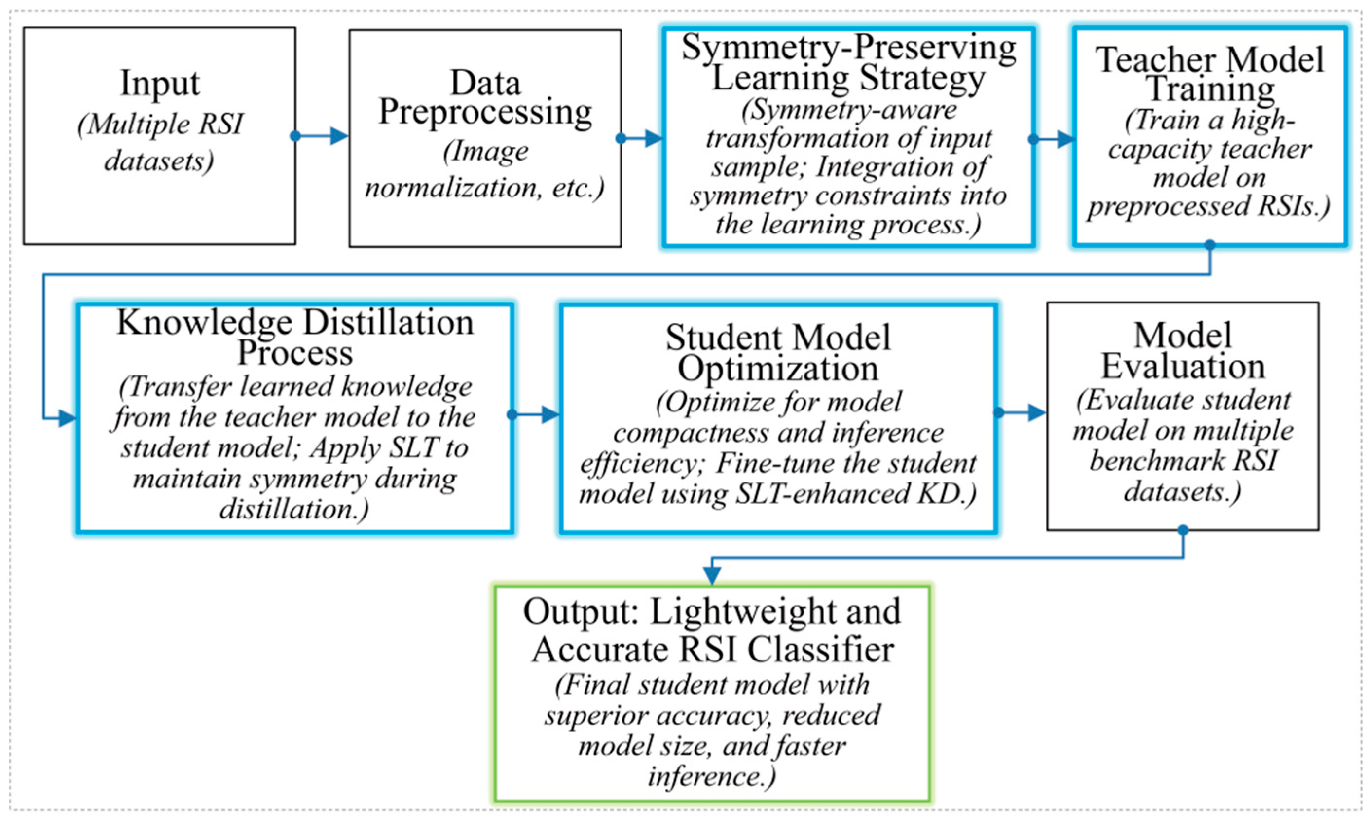
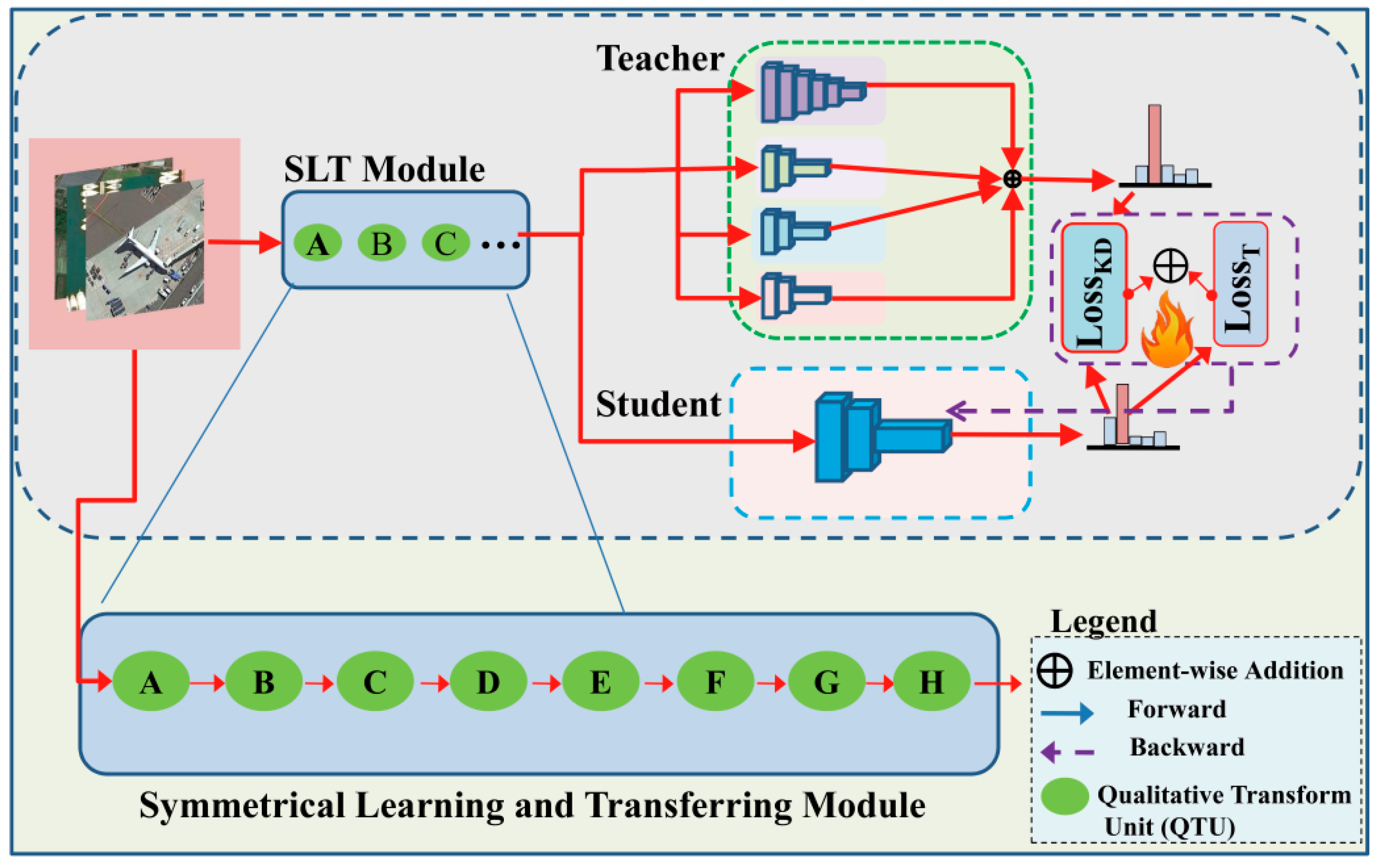
Our Proposed Method	Addresses RSI asymmetries with SLT strategy; achieves superior accuracy, reduced model size (up to 96%), and faster inference (up to 88%) without architectural modifications	Further exploration needed to verify generalization across broader datasets and real-world applications

provides a comparative overview of existing knowledge distillation and lightweight model approaches for RSI classification. It summarizes the main merits and limitations of each category, highlighting their performance in terms of accuracy, model size, and inference efficiency. The comparison shows that most existing methods involve trade-offs between accuracy and model complexity and often fail to achieve both simultaneously. In contrast, our proposed method effectively addresses these limitations by providing superior accuracy, significantly reduced model size, and faster inference without requiring architectural modifications.

3. Methodologies

Figure 4 shows the workflow of the proposed image classification framework. It starts with acquiring multi-source RSI datasets, followed by data preprocessing. The symmetry-preserving learning strategy ensures symmetry during training. A teacher model is trained, and knowledge is distilled into a lightweight, optimized student model. The final model is evaluated for accuracy, size, and inference speed, producing a compact, accurate RSI classifier without architectural changes.

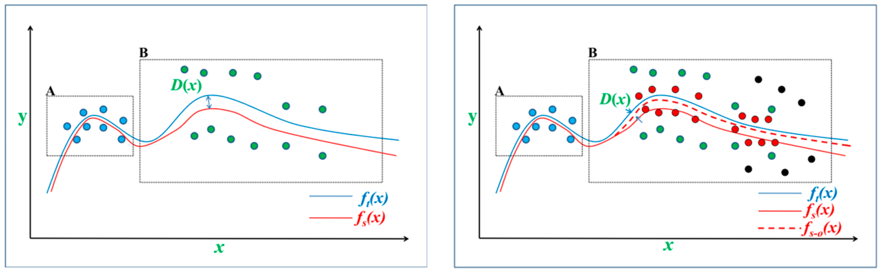
3.1. Qualitative Feature Alignment

Figure 5 illustrates the algorithmic realization of our qualitative feature alignment technique. In this approach, each mini-batch of RSI samples passes through the qualitative transform unit (QTU), which comprises a stochastic probability generator, a conditional branch, and a transformation function. The stochastic probability generator produces a random probability value ($P$) for each batch, sampled from a Gaussian distribution as follows:

$$P\sim \mathcal{N}(\mu ,{\sigma }^2)$$

(1)

where the mean $\mu =0.5$ and the variance ${\mathsf{\sigma }}^2=0.01$ ensure a balanced probability distribution centered around 0.5 with moderate variability. Each sampled probability $P$ is then compared with a predefined threshold ($Th$). If $P\le Th$, the transformation function processes the input features, outputting transformed features that maintain symmetrical consistency. Otherwise, the output features remain identical to the input, preserving their symmetry. This mechanism ensures that, when necessary, feature transformations do not distort the inherent structural relationships within the data.

In a QTU, we denote the input and output features as $X$ and $X^{\prime }$, respectively. We represent the transformation function within this QTU by $f$. Then, the transformation process within the QTU can be described as follows:

$$X^{\prime }=\left\{\begin{array}{l}f(X),\dots if P\le Th\\ X,\dots \dots \dots else\end{array}\right.$$

(2)

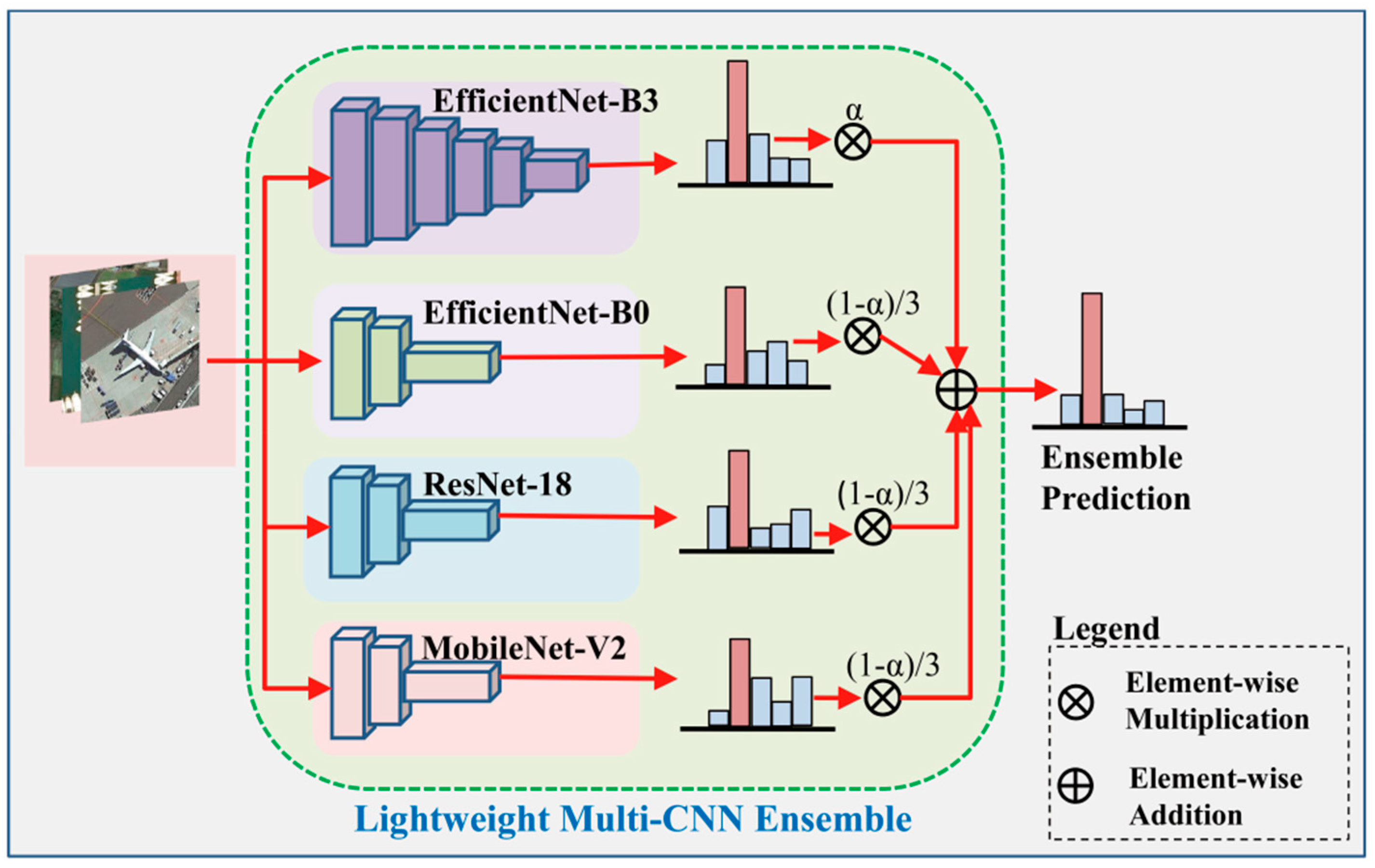
3.2. Architecture of the Teacher Ensemble

Figure 6 illustrates our proposed algorithm for the construction of a multi-CNN ensemble model. This model integrates four distinct CNN models: EfficientNet-B3, EfficientNet-B0, ResNet-18, and MobileNet-V2. For each mini-batch of samples, these CNN classifiers independently generate their prediction logits. These logits are then individually re-weighted through element-wise multiplication with a designated hyperparameter. The final step involves the aggregation of these weighted logits from each CNN, achieved through an element-wise addition, to yield the prediction logits of the teacher ensemble.

We assign the symbol $\alpha$ to represent the hyperparameter for EfficientNet-B3. The logits from the four CNNs and the teacher ensemble are denoted as ${Logit}_{B3}$, ${Logit}_{B0}$, ${Logit}_{R18}$, ${Logit}_{MB}$, and ${Logit}_E$, respectively. Then, the ensemble’s weighted logits can be articulated as follows:

$$Logi{t}_E=\alpha \times Logi{t}_{B3}+\left({\displaystyle \frac{1-\alpha }{3}}\right)\times (Logi{t}_{B0}+Logi{t}_{R18}+Logi{t}_{MB})$$

(3)

In Equation (3), the value of $\alpha$ is selected from the range 0.1 to 0.9 with an interval of 0.1, and the optimal value is determined using the search Algorithm 1 introduced in Section 3.5.

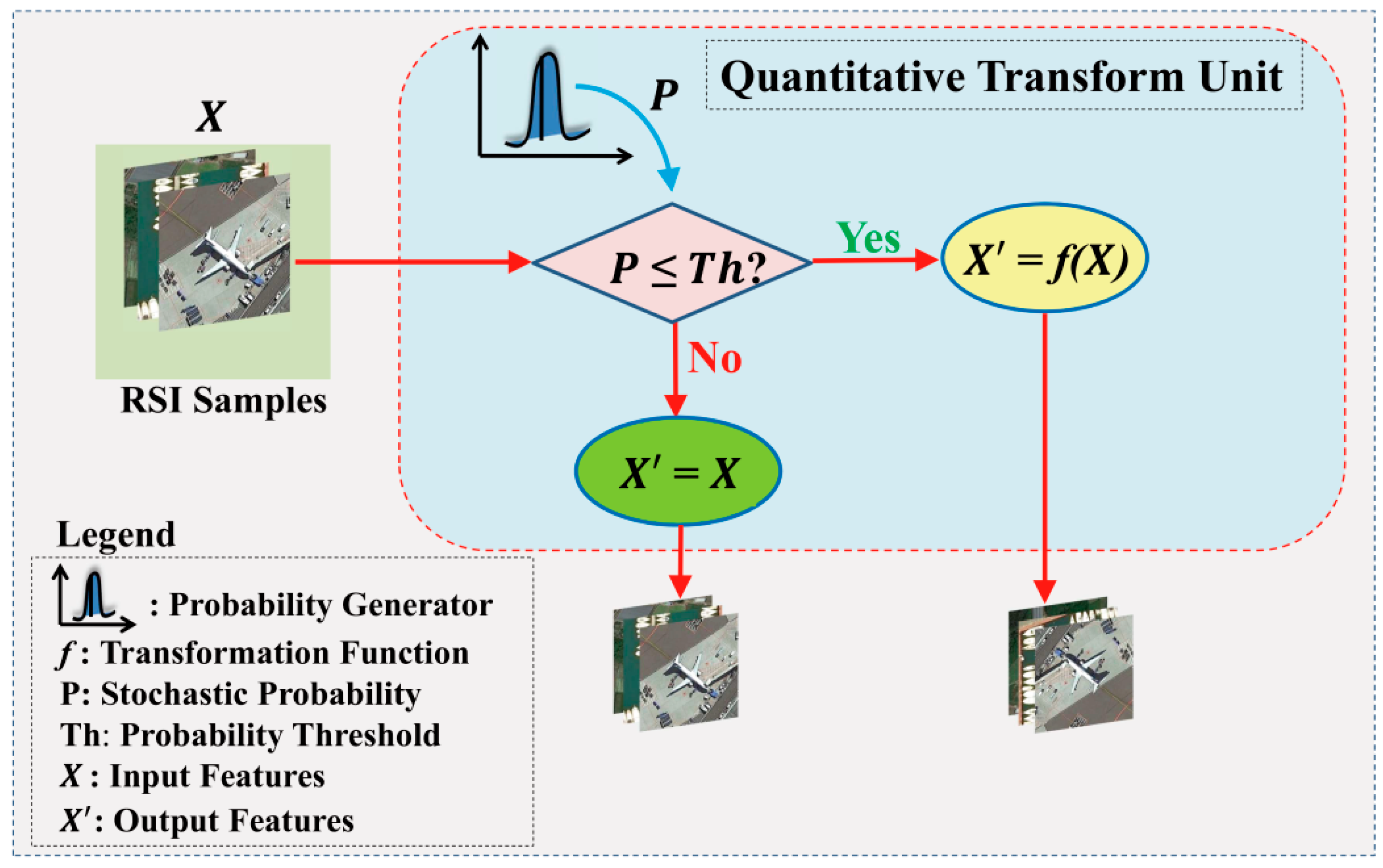
3.3. Symmetrical Learning and Transferring Framework

As illustrated in Figure 7 (see below), the knowledge transferring framework consists of several key steps designed to maintain symmetry in the training process. Initially, the SLT module accepts a batch of original RSIs as input samples, which are then processed through symmetry-aware transformations to either output transformed or unprocessed features. These features are subsequently used as inputs for both the teacher and student models. The teacher and student models generate their respective prediction logits, which are then used to compute the KD loss. Simultaneously, the logits of the student model are compared with the sample labels to compute a training loss. Finally, the KD loss and the training loss are combined via summation to compute gradients.

As shown at the bottom of the figure, the proposed SLT module consists of eight QTUs in sequence, labeled from A to H. Each QTU applies a specific symmetry-preserving transformation or regularization function in the following order: color jitter (A), horizontal flip (B), vertical flip (C), rotation (D), grayscale (E), auto contrast (F), Gaussian blur (G), and CutMix (H). The transformation process for the input sample ($\mathrm{X}$) can be mathematically described as:

$$X^{\prime }=f_H(P_H,f_G(P_G,f_F(P_F,f_E(P_E,f_D(P_D,f_C(P_C,f_B(P_B,f_A(P_A,X))))))))$$

(4)

where $X^{\prime }$ is the final output, $f_A$ to $f_H$ denote the transformation functions, and $P_A$ to $P_H$ are the stochastic probabilities governing each transformation. The probability thresholds within the grayscale and auto-contrast QTUs are set at 0.3, while the thresholds for the remaining QTUs are set at 0.5.

To ensure consistency and preserve symmetry during the KD phase, the training process of each CNN classifier within the teacher ensemble duplicates the same setting for all QTUs. This duplication ensures that the SLT module maintains a symmetrical environment across all teacher models, reducing asymmetries within the training samples. By minimizing these asymmetries, our approach enhances the stability and efficiency of the KD process, ensuring that both the teacher and student models learn from data that is either similarly transformed or untransformed, thereby preserving the structural relationships in the feature space.

3.4. KD Loss

The logit-based method minimizes the prediction difference between the teacher and student models by adjusting their output logits (represented as $Z_i$, where $i$ corresponds to the category number). However, when the teacher model exhibits high confidence, the predictions for target categories can attain values as high as 99%. Consequently, the aggregate of non-target predictions falls below 1%. This scenario leads to significantly low information entropy when transferring knowledge associated with non-target categories.

To address this, researchers commonly introduce a ‘temperature’ hyperparameter (denoted as $t$) to moderate the teacher’s logits. Additionally, the application of cross-entropy loss ($L_{CE}$) between the student’s predictions and the target labels (${Label}_i$) can expedite the KD-based convergence rates.

Consider the prediction logits (denoted as $Z_i$) of a model. In general, these logits are converted into category probabilities (denoted as $P_i$) via a softmax function. In the symbol $P_i$, the subscripts ‘T’ and ‘S’ represent teacher and student, respectively, while a superscript ‘t’ denotes adjustment by temperature. Consequently, we can define the KD loss, denoted as $L_{KD-Training}$, as follows:

$$P_i=softmax \left(Z_i\right)={\displaystyle \frac{exp\left(Z_i\right)}{{{\displaystyle \sum }}_1^{i}exp\left(Z_i\right)}}.$$

(5)

$$P_i^t=softmax({\displaystyle \frac{Z_i}{t}}).$$

(6)

$$L_{CE}=-{{\displaystyle \sum }}_1^i(Labe{l}_i\times log{P}_{S,i})$$

(7)

$$L_{KD-Training}=L_{CE}+{\displaystyle \sum }_1^i(t^2\times P_{T,i}^t\times \log {\displaystyle \frac{P_{T,i}^t}{P_{S,i}^t}})$$

(8)

The squared temperature term ($t^2$) in the equations is included to appropriately scale the gradients produced by the softened probability distributions, maintaining consistent gradient magnitudes and balancing the influence of the distillation loss across different temperature settings [32,33]. However, Stanton et al. [83] argue that a student model, when employing the loss function defined in the equations, struggles to achieve a level of accuracy comparable with that of its highly accurate teacher model. This challenge necessitates an extensive training process, potentially spanning tens of thousands of epochs, before the significant discrepancy in accuracy between the teacher and student models can be rectified.

Recently, Huang et al. [84] introduced an alternative loss function named DIST. This function supersedes the classical KD loss with a Pearson distance, aiming to efficiently align the probability vectors of the teacher ($V_T$) and student models ($V_S$). The definitions of the Pearson correlation coefficient ($\rho$) and the Pearson distance ($D_P$) are as follows:

$$D_P=1-\rho \left(V_T, V_S\right)=1-{\displaystyle \frac{{{\displaystyle \sum }}_0^{\mathrm{i}}(V_T-{\overline{V}}_T)\times \left(V_S-{\overline{V}}_S\right)}{\sqrt{{{\displaystyle \sum }}_0^{\mathrm{i}}{\left(V_T-{\overline{V}}_T\right)}^2\times {{\displaystyle \sum }}_0^{\mathrm{i}}{\left(V_S-{\overline{V}}_S\right)}^2}}}$$

(9)

DIST defines an inter-class loss ($L_{inter}$) and an intra-class loss ($L_{intra}$) based on Equation (9). Suppose the training batch size and category number are denoted by $n$ and $i$, respectively. Then, the DIST loss can be expressed as follows, where ${V_T}^{transpose}$ and ${V_S}^{transpose}$ are the transposes of $V_t$ and $V_s$ at the $n$ and $i$ dimensions:

$$L_{inter}={\displaystyle \frac{1}{n}}{\displaystyle \sum }_1^n{D}_P\left(V_T,V_S\right)$$

(10)

$$L_{intra}={\displaystyle \frac{1}{i}}{\displaystyle \sum }_1^i{D}_P\left({V_T}^{transpose},{V_S}^{transpose}\right)$$

(11)

Moreover, the CutMix technique [85] introduces a modified cross-entropy loss ($L_{CE-CM}$) by integrating two components. This is achieved by replacing a certain proportion of a sample from class A with a patch derived from a sample from class B. If we denote the labels of samples A and B as ${Label}_A$ and ${Label}_B$, respectively, and represent the proportion of the patch as $\beta$, then $L_{CE-CM}$ can be formulated as follows:

$$L_{CE-CM}=\left(1-\beta \right)\times L_{CE}\left(P_S,Labe{l}_A\right)+\beta \times L_{CE}\left(P_S,Labe{l}_B\right)$$

(12)

In this study, we have chosen DIST and $L_{CE-CM}$ as the components of our KD loss. Consistent with the DIST study, we assigned equal weights of 2.0 to both the inter- and intra-loss components and also set the temperature to 2.0. As a result, our KD loss ($\mathrm{d}\mathrm{e}\mathrm{n}\mathrm{o}\mathrm{t}\mathrm{e}\mathrm{d} \mathrm{a}\mathrm{s} L_{KD-proposed}$) can be expressed as follows:

$$L_{KD-proposed}=L_{CE-CM}+2\times L_{inter}+2\times L_{intra}$$

(13)

3.5. Algorithm for Generating the Teacher Ensemble

Algorithm 1 outlines the procedures for generating the teacher ensemble. In particular, our ensemble model employs a fast search method to pinpoint an optimal $\alpha$ among nine possible values. Throughout these cycles, $\alpha$ increases at a rate of 0.1 per cycle. Subsequently, the teacher ensemble uses the optimal $\alpha$ discovered during this search to recalibrate the logits derived from the four CNN classifiers. This approach ensures accuracy and efficiency in the generation of the teacher ensemble.

Algorithm 1. Procedures for Generating the Teacher Ensemble (Pseudocode)
Definition: Let $X_{test}$ represent the testing dataset. Let ${Logit}_E$, ${Logit}_{B3}$, ${Logit}_{B0}$, ${Logit}_{R18}$, ${Logit}_{MB}$, and $\alpha$ represent the same definitions as those in Equation (2).
Input: images and labels from testing subsets. Output: the accuracy ($Acc$) results of the teacher ensemble.
Procedures:
1:	Generate the teacher ensemble using Equation (3), where $\alpha$ is alterable
2:	Initialize $\alpha$ to 0.1.
3:	FOR i = 1 TO 9 DO
4:		Calculate the ensemble’s accuracy on $X_{test}$ using current $\alpha$.
5:		Increment $\alpha$ by 0.1.
6:	END FOR
7:	Return the $Acc$ results along with the corresponding $\alpha$.

3.6. KD Algorithm

The pseudocode in Algorithm 2 outlines the procedure for knowledge transfer between the teacher and student models. As specified in line 1, the process spans 1200 training epochs. Lines 2 and 3 illustrate that during each epoch, a batch of 64 samples, along with their corresponding labels, are simultaneously fed into both the teacher and student models. Subsequently, as delineated in lines 4 to 7, the loss is computed based on the prediction logits from both models. The student model’s parameters are then updated according to the gradients. As depicted in lines 9 and 11, the student model’s accuracy is validated at the conclusion of each epoch, and a record of the accuracy per epoch is compiled upon the completion of the training.

Algorithm 2. Distillation procedures (Pseudocode)
Definitions: The training subset for RSI is denoted as $S_{train}$, while a batch of samples is denoted as $X$. The ensemble teacher model is represented by $f_T$, and the student model is represented by $f_S$. The SLT module is signified by $M_{SLT}$, while $P_T$ and $P_S$ are the same as those in Equation (6).
Input: images and labels from training or testing subsets. Output: the accuracy ($Acc$) results of the student model.
Procedures:
1	FOR Epoch = 1 TO 1200 DO
2		FOR iteration = 1 TO $\left({\displaystyle \frac{length\left(S_{train}\right)}{64}}+1\right)$ DO
3			Sample a batch of samples $X$ from $S_{train}$, and input them to the functions $f_T$ and $f_S$, respectively.
4			Predict teacher probabilities using the equation: $P_T=f_T\left(M_{SLT}\right(X\left)\right)$.
5			Predict student probabilities using the equation: $P_S=f_S\left(M_{SLT}\right(X\left)\right)$.
6			Calculate the loss using Equation (13).
7			Update the student model’s parameters through back propagation.
8		End For
9		Calculate the student model’s accuracy and save this accuracy.
10	End For
11	Return the $Acc$ results

During training, an initial learning rate of 2 × 10⁻⁴ was set and adjusted using the cosine decay algorithm. The Adam-W optimizer was used with a weight decay of 1 × 10⁻⁶. A consistent resolution of 256² was maintained throughout all training and testing stages across all datasets.

3.7. CNN Models

Table 2. Comparative analysis of CNN models employed in this study.

Model	Accuracy (%)	Parameters (M)
EfficientNet-B3	82.0	12.2
EfficientNet-B1	78.6	7.8
EfficientNet-B0	77.6	6.3
ResNet-50	76.1	25.6
ResNet-18	69.7	11.7
MobileNet-V2	72.1	3.5

presents the evaluation of the proposed method using six CNN models. The top one accuracy results, reported by the PyTorch team, are based on the ImageNet-1K dataset. Among these models, EfficientNet-B3, -B1, and -B0, which incorporate built-in channel attention mechanisms, demonstrate superior performance. In contrast, MobileNet-V2 is characterized by its compact size, with only 3.5 million parameters. Detailed descriptions of these model architectures can be found in the reference [6].

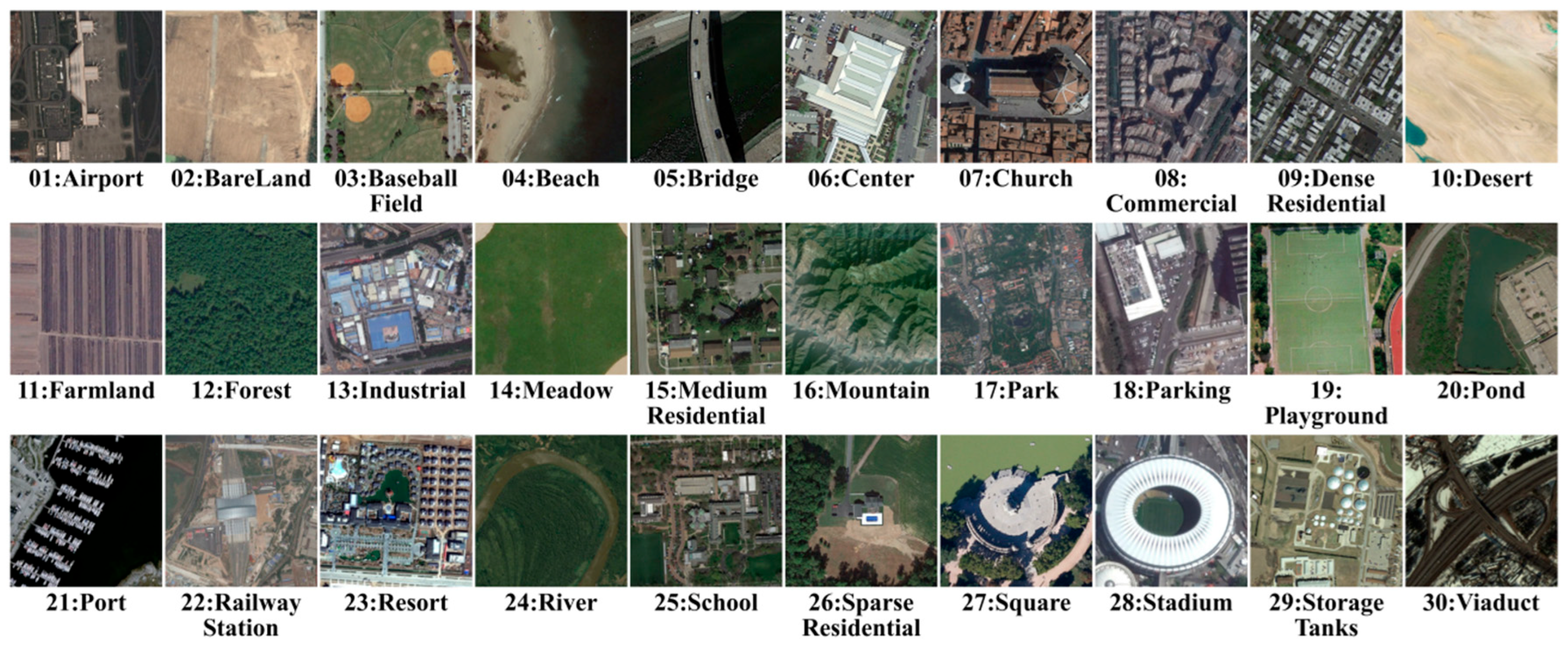
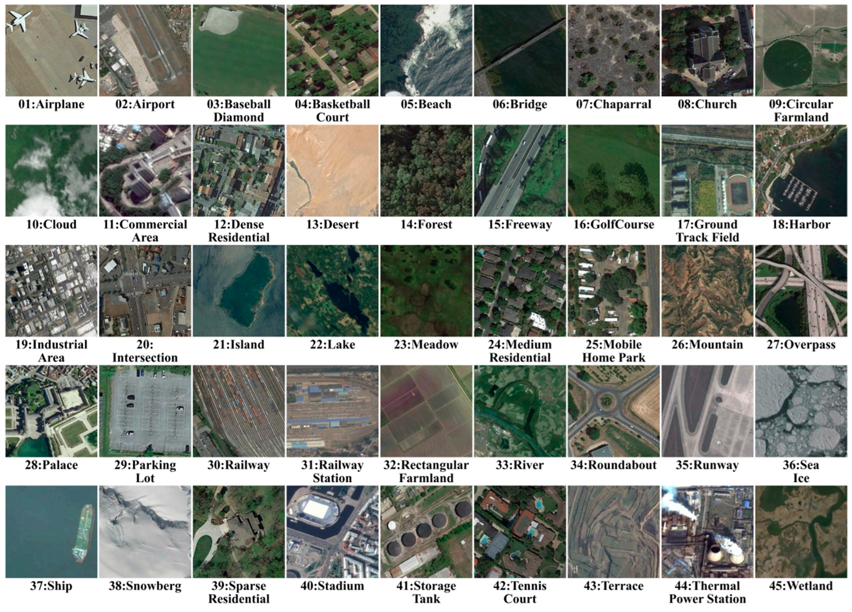
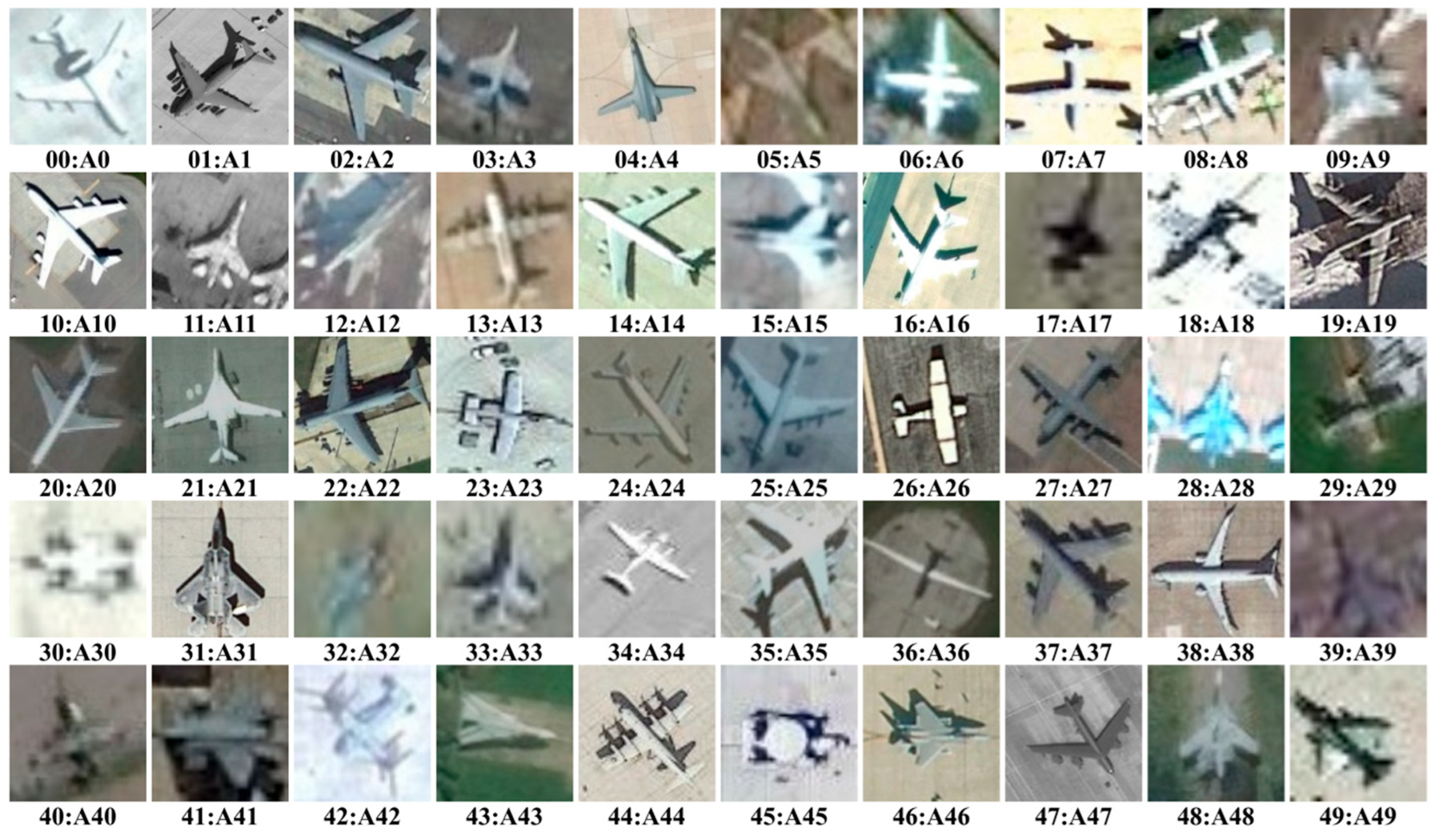
3.8. Dataset and Division

We employed three RSI datasets for performance evaluation: AID30, NWPU45, and AFGR50. All samples in these datasets are cropped from Google Earth imagery, which inherently features varying spatial resolutions and diverse atmospheric conditions. These characteristics closely mirror the complexities of real-world remote sensing data. A detailed summary of these datasets is provided in

Table 3. Comparative summary of three datasets for performance evaluation.

Dataset	Total Classes	Spatial Resolution	Total Images	Image Size	Samples per Class	Training Ratio
AID30 [6]	30	0.5–8 m	10,000	6002 pixels	220–420 (varied)	20%, 50%
NWPU45 [6]	45	30~0.2 m	31,500	2562 pixels	700 (fixed)	10%, 20%
AFGR50 [77]	50	0.5–8 m	12,500	1282 pixels	250 (fixed)	10%, 20%, 30%

.

Generally, the AID30 dataset contains samples with a higher resolution, although the number of samples per category varies. In contrast, the AFGR50 dataset is fine-grained, comprising 50 aircraft categories. The NWPU45 dataset, with its abundant samples, presents a more significant challenge for distinction. Representative samples from each category for the three datasets are provided in Figure A1, Figure A2 and Figure A3 in the Appendix A.

The training ratios in this study follow the official settings commonly used in the literature, ensuring direct and fair comparison with previous studies. Specifically, we use training ratios of 20% and 50% for AID30, 10% and 20% for NWPU45, and 10%, 20%, and 30% for AFGR50. The remaining portions of each dataset are used as testing subsets.

3.9. Performance Evaluation Metrics

In our research, we utilized three performance evaluation metrics: overall accuracy (OA), precision, and the confusion matrix. OA is defined as the ratio of the total number ($N_c$) of samples that were correctly classified to the total number ($N_t$) of classified samples. This can be mathematically represented as follows:

$$OA={\displaystyle \frac{N_c}{N_t}}$$

(14)

Precision measures the proportion of correctly predicted positive samples among all samples predicted as positive, particularly in relation to false positive errors. $TP$ represents the number of true positive predictions and $FP$ denotes the number of false positive predictions. Formally, precision is defined as:

$$Precision={\displaystyle \frac{TP}{TP+FP}}$$

(15)

The confusion matrix is a tabular layout that displays the classification results for all categories within a dataset. It provides a comprehensive overview of the number of samples that have been accurately and inaccurately classified for each category. This matrix is instrumental in understanding the performance of the classification model across different categories.

3.10. Experimental Settings

The experimental procedures were executed on four RTX 4070Ti GPUs. PyTorch version 2.1.0 was utilized within the Ubuntu 20.04 operating system for these experiments. The results reported are mean values derived from at least three independent trials.

4. Experimental Results

4.1. OA Results of the Teacher Ensemble

Table 4. Comparative OAs (%) of various models on three RSI datasets.

Model	AID30		NWPU45		AFGR50
	TR-20%	TR-50%	TR-10%	TR-20%	TR-10%	TR-20%	TR-30%
EfficientNet-B3	97.30 ± 0.06 ↓0.31	98.28 ± 0.07 ↓0.11	94.66 ± 0.17 ↓0.50	96.20 ± 0.08 ↓0.37	93.15 ± 0.61 ↓0.57	96.52 ± 0.13 ↓0.42	97.53 ± 0.10 ↓0.23
EfficientNet-B0	97.05 ± 0.20 ↓0.56	98.17 ± 0.07 ↓0.22	94.45 ± 0.12 ↓0.71	96.01 ± 0.01 ↓0.56	91.58 ± 0.30 ↓2.14	96.11 ± 0.32 ↓0.83	97.37 ± 0.12 ↓0.39
ResNet-18	96.08 ± 0.12 ↓1.53	97.08 ± 0.21 ↓1.21	92.78 ± 0.10 ↓2.38	94.54 ± 0.01 ↓2.03	91.90 ± 0.21 ↓1.82	95.88 ± 0.20 ↓1.06	97.06 ± 0.05 ↓0.70
MobileNet-V2	95.96 ± 0.12 ↓1.65	97.27 ± 0.12 ↓1.19	92.68 ± 0.05 ↓2.48	94.60 ± 0.05 ↓1.97	91.86 ± 0.26 ↓1.86	95.60 ± 0.18 ↓1.34	96.95 ± 0.03 ↓0.81
Teacher Ensemble	97.61 ± 0.04	98.39 ± 0.10	95.16 ± 0.19	96.57 ± 0.01	93.72 ± 0.40	96.94 ± 0.15	97.76 ± 0.04

illustrates the OA results of our teacher ensemble, along with its four CNN components. The values highlighted by arrows indicate an OA decrease compared with the ensemble model.

Firstly, Table 4 shows that the OA gaps between all models are minimal for those training ratios (TRs) that contain ample training samples, such as the TR-50% of AID30 or the TR-30% of AFGR50. This suggests that models can easily reach saturation on these larger TRs, despite ResNet-18 and MobileNet-V2 exhibiting noticeably lower accuracy on other smaller TRs.

Secondly, when compared with ResNet-18 and MobileNet-V2, we observe that EfficientNet-B3 and -B0, the top two models among the four CNNs, exhibit significant accuracy improvements on the AID30 and NWPU45 datasets. However, when the image quality deteriorates to a low resolution, as in the case of the AFGR50 dataset, those relative accuracy improvements associated with EfficientNet-B3 or B0 both decrease. This indicates that the recognition of fine-grained objects differs from other common tasks.

Lastly, when compared with EfficientNet-B3, the results demonstrate that our teacher ensemble consistently introduces approximately 0.3 to 0.6 improvements in accuracy across different datasets. This validates the effectiveness of our straightforward algorithm for generating lightweight ensembles by enhancing the accuracy of individual CNNs.

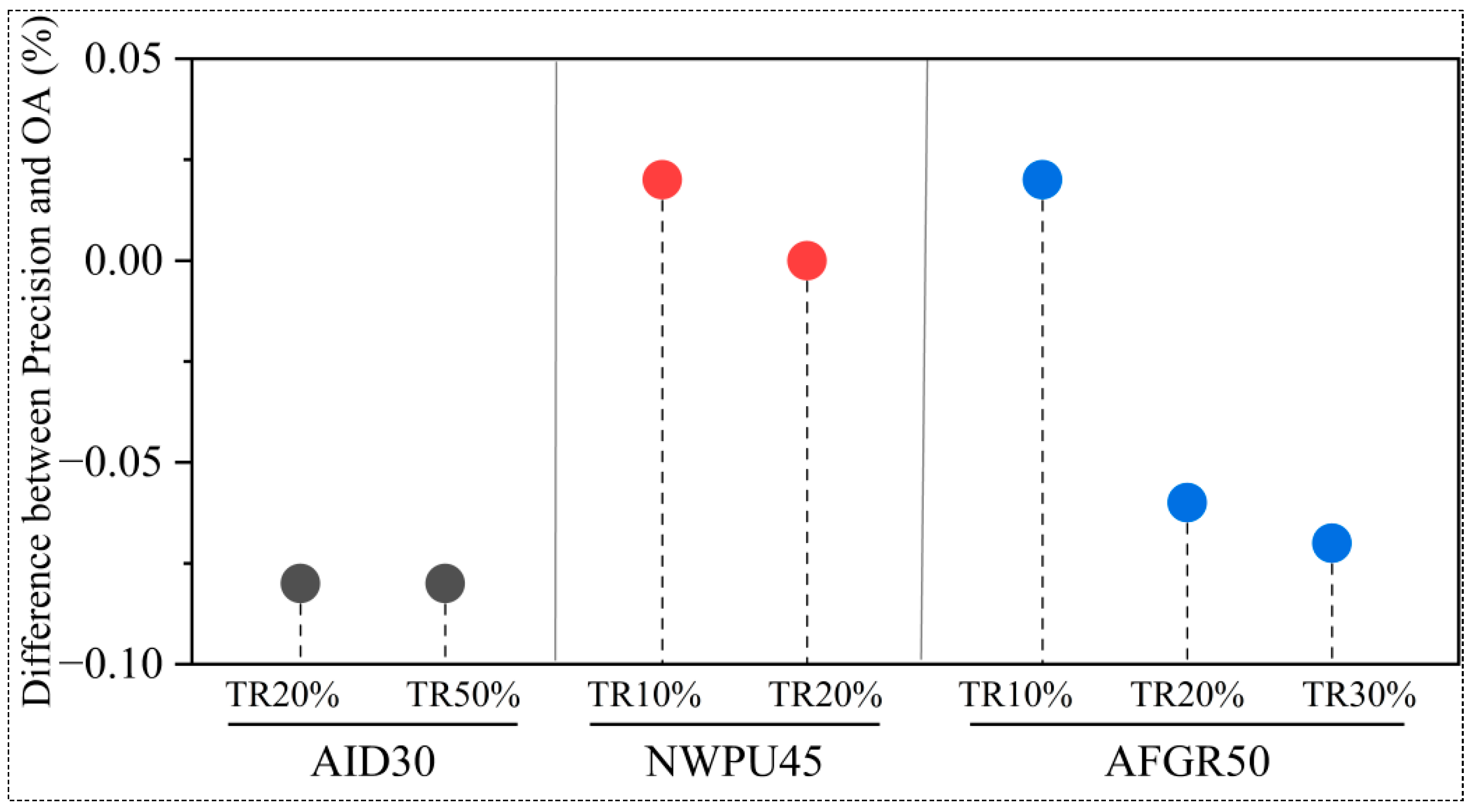
Sensitivity Analysis of the Ensemble Configuration

Typically, an ensemble model achieves enhanced accuracy when its constituent models are both diverse and precise. To analyze the sensitivity of our ensemble generation algorithm, we substituted two components from our teacher model, EfficientNet-B0 and ResNet-18, with EfficientNet-B1 and ResNet-50, respectively.

Table 5. Comparative analysis of OA (%) across different ensemble configurations.

Model	AID30		NWPU45		AFGR50
	TR-20%	TR-50%	TR-10%	TR-20%	TR-10%	TR-20%	TR-30%
EfficientNet-B1	97.14 ± 0.11 ↑0.09	98.16 ± 0.07 ↓0.01	94.45 ± 0.12 ↑0.0	96.03 ± 0.01 ↑0.02	91.27 ± 0.34 ↓0.31	95.97 ± 0.18 ↓0.14	97.23 ± 0.05 ↓0.14
ResNet-50	96.08 ± 0.12 ↑0.0	97.08 ± 0.21 ↑0.0	92.78 ± 0.10 ↑0.0	94.54 ± 0.01 ↑0.0	92.33 ± 0.32 ↑0.43	96.13 ± 0.22 ↑0.25	97.25 ± 0.14 ↑0.19
Teacher Ensemble (heavy)	97.63 ± 0.07 ↑0.02	98.39 ± 0.08 ↑0.0	95.08 ± 0.14 ↓0.08	96.58 ± 0.06 ↑0.01	93.96 ± 0.45 ↑0.24	96.89 ± 0.15 ↓0.05	97.73 ± 0.01 ↓0.03

presents the OA results of this modified ensemble, referred to as ‘heavy’, along with its new components. The values highlighted by arrows represent a decrease or increase in accuracy, respectively, compared with those in Table 4. The compared pairs include EfficientNet-B1 versus B0, ResNet-50 versus 18, and the modified ensemble versus the original ensemble.

As Table 5 demonstrates, ResNet-50 marginally outperforms ResNet-18 in terms of OA on the AFGR50 dataset. However, the enhancements on the AID30 and NWPU45 datasets are minimal. Similarly, EfficientNet-B1 shows only slight OA improvements across all three datasets. The ‘heavy’ teacher ensemble, a modified version of the original, does not yield significant OA advancements. These observations indicate that our ensemble generation algorithm is resilient to moderate alterations in the size of the component models. Therefore, due to its reduced size, we designate the original ensemble as the teacher model of choice.

4.2. OA Results of the Student Models

Table 6. Comparative OAs (%) of various student models on three RSI datasets.

Model	Params (M)	AID30		NWPU45		AFGR50
		TR-20%	TR-50%	TR-10%	TR-20%	TR-10%	TR-20%	TR-30%
Teacher Ensemble	33.7	97.61 ± 0.04	98.39 ± 0.10	95.16 ± 0.19	96.57 ± 0.01	93.72 ± 0.40	96.94 ± 0.15	97.76 ± 0.04
Student (MobileNet-V2)	3.5	96.69 ± 0.06 ↓0.92	97.77 ± 0.09 ↓0.62	93.79 ± 0.03 ↓1.37	95.49 ± 0.07 ↓1.08	93.10 ± 0.30 ↓0.62	96.34 ± 0.24 ↓0.60	97.52 ± 0.04 ↓0.24
Student (ResNet-18)	11.7	96.55 ± 0.22 ↓1.06	97.45 ± 0.22 ↓0.94	93.70 ± 0.09 ↓1.46	95.35 ± 0.04 ↓1.22	93.13 ± 0.36 ↓0.59	96.32 ± 0.18 ↓0.62	97.50 ± 0.06 ↓0.26
Student (EfficientNet-B0)	6.3	97.32 ± 0.06 ↓0.29	98.24 ± 0.05 ↓0.15	94.70 ± 0.04 ↓0.46	96.34 ± 0.11 ↓0.23	93.15 ± 0.31 ↓0.57	96.55 ± 0.26 ↓0.39	97.79 ± 0.05 ↑0.03
Student (EfficientNet-B1)	7.8	97.44 ± 0.05 ↓0.17	98.34 ± 0.09 ↓0.05	94.97 ± 0.09 ↓0.19	96.43 ± 0.01 ↓0.14	93.29 ± 0.33 ↓0.43	96.64 ± 0.23 ↓0.30	97.73 ± 0.03 ↓0.03

showcases the OA results of four student models, each of which is a lightweight CNN. The values highlighted by arrows signify a decrease or increase in accuracy, respectively, relative to the teacher model.

The data in the table indicates that all four lightweight CNNs have successfully absorbed knowledge from their teacher during the KD process. Notably, MobileNet-V2 and ResNet-18 exhibit larger OA discrepancies with their teachers, while those of EfficientNet-B1 and -B0 are very minimal. Furthermore, the OA differences on the AFGR50 dataset among various student CNNs are less pronounced than those on the AID30 and NWPU45 datasets. This suggests that our SLT strategy can effectively impart knowledge from the ensemble teacher to a variety of lightweight CNNs, regardless of their architectural differences. It is also evident that the efficiency of knowledge transfer is strongly tied to the inherent classification capabilities of the student models. However, when addressing fine-grained RSIs such as those in the AFGR50 dataset, the efficiency of KD exhibits only a weak correlation with the classification capabilities of the student models. We attribute this phenomenon to the limited general features present within low-quality images.

Analysis of Ensemble Configuration Sensitivity on KD Efficiency

Table 7. Comparative analysis of OAs (%) for student models supervised by the ‘heavy’ teacher model.

Model	Params (M)	AID30		NWPU45		AFGR50
		TR-20%	TR-50%	TR-10%	TR-20%	TR-10%	TR-20%	TR-30%
Teacher Ensemble (heavy)	33.7	97.63 ± 0.07	98.39 ± 0.08	95.08 ± 0.14	96.58 ± 0.06	93.96 ± 0.45	96.89 ± 0.15	97.73 ± 0.01
Student (MobileNet-V2)	3.5	96.56 ± 0.09 ↓1.07	97.66 ± 0.10 ↓0.73	93.66 ± 0.11 ↓1.42	95.33 ± 0.04 ↓1.25	93.04 ± 0.27 ↓0.92	96.24 ± 0.22 ↓0.65	97.49 ± 0.10 ↓0.24
Student (ResNet-18)	11.7	96.25 ± 0.10 ↓1.38	97.35 ± 0.09 ↓1.04	93.43 ± 0.04 ↓1.65	95.17 ± 0.04 ↓1.41	92.93 ± 0.43 ↓1.03	96.26 ± 0.20 ↓0.63	97.50 ± 0.09 ↓0.23
Student (EfficientNet-B0)	6.3	97.22 ± 0.06 ↓0.41	98.26 ± 0.08 ↓0.13	94.66 ± 0.10 ↓0.42	96.31 ± 0.05 ↓0.27	93.23 ± 0.34 ↓0.73	96.63 ± 0.18 ↓0.26	97.77 ± 0.02 ↑0.04
Student (EfficientNet-B1)	7.8	97.43 ± 0.12 ↓0.20	98.22 ± 0.13 ↓0.17	94.89 ± 0.04 ↓0.19	96.43 ± 0.02 ↓0.15	93.20 ± 0.26 ↓0.76	96.57 ± 0.16 ↓0.32	97.63 ± 0.02 ↓0.10

delineates the OA results for four distinct student models when the supervisory role during the KD phase is assumed by the ‘heavy’ teacher model. The values highlighted by arrows represent an increase or decrease in accuracy, respectively, when compared with the teacher model.

The information in the table indicates that the four student CNNs are capable of acquiring knowledge from the heavy teacher. Moreover, the inherent classification capabilities of student models, when superior, lead to an increase in the efficiency of knowledge transfer from the teacher. This observation underscores the robustness of our KD strategy across a variety of teacher ensemble configurations.

Additionally, as indicated in Table 7, the OAs of the four student CNNs are marginally lower than those presented in Table 6, where the student models are under the supervision of a teacher ensemble with a smaller model size. This observation aligns with the findings of the referenced study [86], suggesting that larger discrepancies in model sizes between a teacher and a student can lead to significant differences in OA between the models following the KD process.

4.3. Performance Comparison with Previous KD Methods

Table 8. Comparative analysis of OA (%) among the proposed and previous KD methods.

Model	Tech. Approach	Pub. Year	Params (M)	AID30		NWPU45
				TR-20%	TR-50%	TR-10%	TR-20%
GeNet2B [38]	Logit- Based	2021	1.7	80.97 ± 0.01 ↓16.46	None	None	None
PWS-Net [39]		2022	21.8	91.57 (TR equals 50%) ↓6.65		94.77 (TR equals 70%) ↓1.66
ETGS-Net [40]		2022	11.7	95.58 ± 0.18 ↓1.85	96.88 ± 0.19 ↓1.34	92.72 ± 0.28 ↓2.17	94.50 ± 0.18 ↓1.93
DKD-Net [41]	Feature- Based	2022	4.4	95.09 ↓2.43	96.94 ↓1.28	93.72 ↓1.17	95.76 ↓0.67
A2N-Net [42]		2023	>143.7	84.20 ± 0.39 ↓13.43	None	None	None
DCN-Net [43]		2023	None	94.94 ± 0.16 ↓2.49	97.34 ± 0.18 ↓0.88	94.58 ± 0.18 ↓0.31	95.80 ± 0.12 ↓0.63
CKD-Net [45]		2022	>90.0	None	None	None	91.60 ↓4.83
EMSC-Net [44]	Contrastive Learning with KD	2023	173.6	96.02 ± 0.18 ↓1.41	97.35 ± 0.17 ↓0.87	93.58 ± 0.22 ↓1.31	95.37 ± 0.07 ↓1.06
LaST-Net [46]	Self- Distillation	2022	28.3	83.23 ↓14.2	87.34 ↓10.88	72.58 ↓22.31	73.67 ↓22.76
VSD-Net [47]		2022	>8.0	96.73 ± 0.15 ↓0.70	97.95 ± 0.10 ↓0.27	93.24 ± 0.11 ↓1.65	95.67 ± 0.11 ↓0.76
ESDMBE-Net [48]		2022	92.5	96.00 ± 0.15 ↓1.43	98.54 ± 0.17 ↑0.32	94.32 ± 0.15 ↓0.57	95.58 ± 0.08 ↓0.85
SSKD-Net [49]		2022	77.2	95.96 ± 0.12 ↓1.47	97.45 ± 0.19 ↓0.77	92.77 ± 0.05 ↓2.12	94.92 ± 0.12 ↓1.51
FASD-Net [50]		2023	24.8	96.05 ± 0.13 ↓1.38	97.84 ± 0.12 ↓0.38	92.89 ± 0.13 ↓2.00	94.95 ± 0.12 ↓1.48
CASD-ViT [51]		2024	86.0	96.18 ± 0.20 ↓1.25	97.64 ± 0.11 ↓0.58	93.12 ± 0.12 ↓1.77	95.52 ± 0.16 ↓0.91
Teacher Ensemble	Logit- Based	Ours	33.7	97.63 ± 0.07	98.39 ± 0.08	95.08 ± 0.14	96.58 ± 0.06
Student-B0			6.3	97.22 ± 0.06	98.26 ± 0.08	94.66 ± 0.10	96.31 ± 0.05
Student-B1			7.8	97.43 ± 0.12	98.22 ± 0.13	94.89 ± 0.04	96.43 ± 0.02

provides a comparative analysis of the OA results for our student EfficientNet-B1, -B0 (also referred to as student-B0 and -B1), and 14 other KD-based models cited in the literature. The values highlighted by arrows indicate a decrease or increase in OA, respectively, in comparison with our EfficientNet-B1 model. ‘None’ in the table means no disclosed data in the literature.

The information presented in the table demonstrates that our student-B1 model surpasses other logit-based methods, with an accuracy enhancement of up to 16.5%. Simultaneously, our student-B1 model also outperforms other feature-based or self-distillation methods, with an OA improvement of up to 13.4% and 22.8%, respectively. Furthermore, both our student-B1 and -B0 models deliver superior accuracy while maintaining a competitive model size. By contrast, only ESDMBE-Net [48] exhibits an OA increase of approximately 0.32% on the TR-50% of the AID30 dataset, even though its model size is 12 times larger than our student-B1 model. This comparison thus validates that our method offers a more efficient approach for developing accurate and lightweight classifiers for RSIs.

4.3.1. Performance Comparison with Previous Single-Model Methods

Table 9. Comparative analysis of OA (%) among the proposed and other single-model methods.

Model	Tech. Approach	Pub. Year	Params (M)	AID30		NWPU45
				TR-20%	TR-50%	TR-10%	TR-20%
B3Attn-Net [53]	EfficientNet Reinforcement	2021	>12.2	94.45 ± 0.76	96.56 ± 0.12	None	None
ERA-Net [54]		2021	>6.3	95.93 ± 0.13	98.39 ± 0.16 ↑0.17	91.95 ± 0.19	95.12 ± 0.17
LSRL-Net [55]		2022	None	96.44 ± 0.10 ↓0.99	97.36 ± 0.21	93.45 ± 0.16	94.27 ± 0.44
B7Mod-Net [56]		2023	66.3	94.63	97.46	None	None
QSS-Net [57]		2023	12.2	95.71	None	93.98 ↓0.91	94.71 ↓1.72
LDBST-Net [58]	Swin- Transformer Reinforcement	2023	38.4	95.10 ± 0.09	96.84 ± 0.20	93.86 ± 0.18	94.36 ± 0.12
SwinHCST [59]		2023	None	93.60 (TR equals 70%)		93.76 (TR equals 70%)
HFFT-Swin [60]		2023	29.3	97.08 ± 0.53	97.91 ± 0.27	93.98 ± 0.43	95.98 ± 0.26 ↓0.45
IBSW-Net [61]		2023	164.0	97.61 ± 0.12 ↑0.18	98.78 ± 0.09 ↑0.56	93.98 ± 0.24 ↓0.91	95.65 ± 0.11
MFST-Net [62]		2022	30.8	96.23 ± 0.16	97.38 ± 0.08	92.64 ± 0.08	94.90 ± 0.06
CAF-Net [63]		2024	None	None	None	94.12 (TR equals 80%)
CSCA-Net [64]	CNN Reinforcement	2023	>21.8	94.67 ± 0.20	96.83 ± 0.14	91.27 ± 0.11	93.72 ± 0.10
PSCLI-Net [65]		2024	26.6	96.28	97.52	92.92	94.86
EAM-Net [66]		2024	>25.6	93.14	95.39	90.38	93.04
FSC-Net [67]		2024	28.8	95.56 ± 0.07 ↓1.87	97.51 ± 0.03 ↓0.71	93.03 ± 0.02 ↓1.86	94.76 ± 0.03 ↓1.67
MCAF-Net [68]		2023	None	93.72 ± 0.28	96.06 ± 0.29	91.97 ± 0.24	93.86 ± 0.17
BSN-Net [69]		2023	None	94.06 (TR equals 80%)		95.93 (TR equals 80%)
Bayes-Net [70]	New CNN Architecture	2024	949.9	None	97.57	96.44 (TR equals 50%)
FSA-Net [71]		2024	18.6	None	None	91.7 (TR equals 50%)
JF-Net [72]		2023	5.0	93.05 ± 0.46 ↓4.38	96.65 ± 0.15 ↓1.57	91.36 ± 0.29 ↓3.53	93.25 ± 0.16 ↓3.18
MGhost-Net [73]		2023	5.7	92.05 (TR equals 50%)		91.73 (TR equals 50%)
ViT-CL [74]	ViT Reinforcement	2023	86.6	95.60 ↓1.83	97.42 ↓0.90	92.85 ↓2.04	94.69 ↓1.74
RFD-Net [75]		2023	30.0	None	None	96.29 (TR equals 80%)
Teacher Ensemble	Logit- Based	Ours	33.7	97.63 ± 0.07	98.39 ± 0.08	95.08 ± 0.14	96.58 ± 0.06
Student-B0			6.3	97.22 ± 0.06	98.26 ± 0.08	94.66 ± 0.10	96.31 ± 0.05
Student-B1			7.8	97.43 ± 0.12	98.22 ± 0.13	94.89 ± 0.04	96.43 ± 0.02

provides a comparison of OA between our student models and 23 other single-model methods reported in the literature. We divided these previous studies into five categories, and bold values represent the highest OAs within each category. Furthermore, values highlighted by arrows indicate a decrease or increase in OA, respectively, compared with our student-B1 model. The term ‘None’ signifies that no data was disclosed in the respective literature.

The data in the table reveals that our student-B1 model outperforms all other methods, demonstrating substantial increases in OA, with the exception of ERA-Net [54] and IBSW-Net [61]. These two models exhibit a minor OA improvement on the AID30 dataset. However, it is likely that models reach saturation at the TR50% level due to the availability of ample training samples. Consequently, we argue that only IBSW-Net exhibits an identification capability for the AID30 dataset comparable with our student-B1 model, despite the former having 21 times more parameters than ours. This is because the OAs of ERA-Net markedly decrease as the TRs decline. Nevertheless, when using the accuracies on the challenging NWPU45 dataset as benchmarks, our solution unequivocally surpasses all single-model methods published in the past three years.

Specifically, when our student-B1 model is contrasted with methods that incorporate an EfficientNet architecture, it exhibits noticeable enhancements in OA. This observation underscores the effectiveness of our SLT strategy over other reinforcement strategies. In essence, this finding signifies that the strengths of our approach are not solely derived from the inherent architectural benefits of EfficientNets.

4.3.2. Performance Comparison with Previous Multi-Model Methods

Table 10. Comparative analysis of OA (%) among the proposed and other multi-model methods.

Model	Pub. Year	Params (M)	AID30		NWPU45		AFGR50
			TR-20%	TR-50%	TR-10%	TR-20%	TR-10%	TR-20%	TR-30%
MBC-Net [15]	2024	17.3	97.39 ± 0.01 ↓0.04	98.35 ± 0.09	94.85 ± 0.04	96.40 ± 0.06 ↓0.03	91.01 ± 0.61 ↓2.28	96.13 ± 0.26 ↓0.51	97.28 ± 0.27 ↓0.45
L2RCF-Net [76]	2023	46.7	97.00 ± 0.17	97.80 ± 0.22	94.58 ± 0.16	95.60 ± 0.12	None	None	None
P2FEViT [77]	2023	>112.2	None	None	94.97 ± 0.13 ↑0.08	95.74 ± 0.19	89.30 ± 0.07	94.78 ± 0.15	97.12 ± 0.09
MSE-Net [78]	2024	61.4	96.30 ± 0.10	97.00 ± 0.17	92.80 ± 0.17	94.70 ± 0.16	None	None	None
SFMS-Former [79]	2023	36.3	96.68 ± 0.64	98.57 ± 0.23	92.74 ± 0.23	94.85 ± 0.13	None	None	None
SER-Net [80]	2023	None	None	None	93.31 ± 0.16	95.40 ± 0.13	None	None	None
CKRL-Net [81]	2024	>113.4	97.08 ± 0.12	98.16 ± 0.21	94.60 ± 0.10	95.88 ± 0.17	None	None	None
TST-Net [82]	2022	173.0	97.20 ± 0.22	98.70 ± 0.12 ↑0.48	94.08 ± 0.24	95.70 ± 0.10	None	None	None
Teacher Ensemble	Ours	33.7	97.63 ± 0.07	98.39 ± 0.08	95.08 ± 0.14	96.58 ± 0.06	93.72 ± 0.40	96.94 ± 0.15	97.76 ± 0.04
Student-B0		6.3	97.22 ± 0.06	98.26 ± 0.08	94.66 ± 0.10	96.31 ± 0.05	93.15 ± 0.31	96.55 ± 0.26	97.79 ± 0.05
Student-B1		7.8	97.43 ± 0.12	98.22 ± 0.13	94.89 ± 0.04	96.43 ± 0.02	93.29 ± 0.33	96.64 ± 0.23	97.73 ± 0.03

displays the OA results of our methods, juxtaposed with eight previous strategies that employ a multi-model approach. The values highlighted by arrows, along with ‘None’, carry the same definition as those in Table 8.

The data in the table indicates that MBC-Net [15] and P2FEViT [77] hold the top ranks among these multi-model methods, as other models exhibit a significant drop in accuracy. Furthermore, SFMS-Former [79] and TST-Net [82] only demonstrate competitive accuracy for the TR of 50% in the AID30 dataset, but their accuracy significantly diminishes for other TRs. In contrast, our student-B1 model still achieves superior accuracy for the fine-grained AFGR50 dataset, with noticeable OA improvements over MBC-Net and P2FEViT. This finding underscores the robustness of our SLT strategy for RSI classification.

4.3.3. Model Precision Analysis

Figure 8 (shown below) presents a comparative analysis of the difference obtained by subtracting OA from precision for the proposed student-B1 model across the AID30, NWPU45, and AFGR50 datasets. The differences between precision and OA remain minimal for all configurations, with values consistently falling within a narrow range from 0.0 to −0.08. This alignment of these metrics indicates that false positives occur at a minimal rate and do not significantly impact model performance.

4.4. Ablation Experiments

4.4.1. Efficacy of Qualitative Feature Alignment

Table 11. Impact of qualitative feature alignment on single-CNN model training (OA, %).

Model	Parameter Settings (Operation Prob. = 1.0)	AID30	NWPU45	AFGR50
		TR-20%	TR-10%	TR-10%
EfficientNet-B3	Color Jitter	97.32 ± 0.12 ↑0.02	94.57 ± 0.07 ↓0.09	93.04 ± 0.73 ↓0.11
	Horizontal Flip	97.26 ± 0.05 ↓0.04	94.64 ± 0.11 ↓0.02	92.78 ± 0.61 ↓0.37
	Vertical Flip	97.21 ± 0.02 ↓0.09	94.63 ± 0.21 ↓0.03	92.75 ± 0.35 ↓0.04
	Random Rotation	97.14 ± 0.11 ↓0.16	94.46 ± 0.12 ↓0.20	92.74 ± 0.36 ↓0.40
	Random Grayscale	17.50 ± 1.11 ↓79.8	47.93 ± 6.33 ↓46.7	43.31 ± 6.43 ↓0.04
	Auto Contrast	97.15 ± 0.11 ↓0.15	94.49 ± 0.12 ↓0.17	92.89 ± 0.43 ↓49.8
	Gaussian blur	97.29 ± 0.01 ↓0.01	94.55 ± 0.10 ↓0.11	92.81 ± 0.52 ↓0.04
	CutMix	97.25 ± 0.08 ↓0.05	94.51 ± 0.08 ↓0.15	92.77 ± 0.33 ↓0.34
	Our SLT	97.30 ± 0.06	94.66 ± 0.17	93.15 ± 0.61

showcases the outcomes of the initial set of ablation experiments. These were designed to assess the qualitative configuration of hyperparameters within our SLT strategy. More specifically, we sequentially adjusted the probability of each QTU within the SLT module to 1.0. This adjustment aimed to evaluate the influence of each transformation on the training process of a single-CNN model, under the assumption that these transformations are persistently activated, which is a common practice in qualitative DA strategies. To minimize interference from model saturation on larger TRs, we selected smaller TRs from three datasets for testing. The values highlighted by arrows signify a decrease or increase in OA, respectively.

The table’s data reveals that the persistent activation of the grayscale transformation during training significantly diminishes the model’s OA. Conversely, when other transformations are persistently activated during training, EfficentNet-B3 consistently exhibits a minor decline in OA, although the color jitter transformation results in a slight positive impact on the AID30 dataset. Moreover, the decrease in OA is more noticeable in the fine-grained AFGR50 dataset compared with the AID30 or NWPU45 datasets. These observations imply that our SLT strategy favors quantitative selections for training single CNNs.

Table 12. Impact of qualitative feature alignment on student-B1 during KD processes (OA, %).

Model	Parameter Settings (Operation Prob. = 1.0)	AID30	NWPU45	AFGR50
		TR-20%	TR-10%	TR-10%
Student-B1	Color Jitter	97.47 ± 0.08 ↑0.03	94.88 ± 0.09 ↓0.09	93.19 ± 0.39 ↓0.20
	Horizontal Flip	97.41 ± 0.03 ↓0.03	94.91 ± 0.05 ↓0.06	93.26 ± 0.32 ↓0.03
	Vertical Flip	97.42 ± 0.06 ↓0.02	94.86 ± 0.06 ↓0.11	93.22 ± 0.31 ↓0.07
	Random Rotation	97.29 ± 0.10 ↓0.15	94.80 ± 0.11 ↓0.17	93.04 ± 0.29 ↓0.25
	Random Grayscale	90.14 ± 3.92 ↓7.30	92.56 ± 0.38 ↓2.41	87.12 ± 0.40 ↓10.2
	Auto Contrast	97.36 ± 0.09 ↓0.08	94.83 ± 0.08 ↓0.14	93.16 ± 0.29 ↓0.13
	Gaussian blur	97.42 ± 0.03 ↓0.02	94.88 ± 0.09 ↓0.09	93.16 ± 0.27 ↓0.13
	CutMix	97.38 ± 0.11 ↓0.06	94.85 ± 0.08 ↓0.12	93.37 ± 0.32 ↑0.08
	Our SLT	97.44 ± 0.05	94.97 ± 0.09	93.29 ± 0.33

delineates the outcomes of the second series of ablation experiments, presented in a format identical to that of Table 11. However, the objective of this test is to assess the impact of each transformation on the student-B1 model during the KD process. The table’s information demonstrates that maintaining the grayscale transformation in an active state significantly reduces the student model’s accuracy. At the same time, minor improvements in the student model’s OA are observed on the AID30 and NWPU45 datasets when the color jitter and CutMix transformations are persistently activated. However, the predominant trend across the majority of the experimental results indicates that the SLT strategy yields inferior results during the KD processes when it incorporates qualitative selections within its functional units. This observation underscores the effectiveness of our SLT strategy in utilizing quantitative choices during KD processes.

Table 13. Impact of removal of quantitative feature alignment on student-B1 during KD processes (OA, %).

Model	Parameter Settings (Operation Prob. = 1.0)	AID30	NWPU45	AFGR50
		TR-20%	TR-10%	TR-10%
Student-B1	H-flip + V-flip	96.43 ± 0.13 ↓1.01	93.61 ± 0.06 ↓1.36	84.63 ± 0.46 ↓8.66
	H-flip + V-flip + CutMix	97.32 ± 0.11 ↓0.12	94.49 ± 0.08 ↓0.48	91.06 ± 0.05 ↓2.23
	Our SLT	97.44 ± 0.05	94.97 ± 0.09	93.29 ± 0.33

presents the results of the third series of ablation experiments, following the same format as Table 11 and Table 12. The aim of this test is to evaluate the effectiveness of the qualitative feature alignment technique when used to transfer knowledge between our teacher and student models. Specifically, we replicate two sets of transformation combinations frequently used in prior studies, including the first set with consistently active horizontal flip (H-flip) and vertical flip (V-flip) and the second set with consistently active H-Flip, V-Flip, and CutMix.

The findings presented in Table 13 indicate that when only the horizontal flip (H-flip) and vertical flip (V-flip) transformations are qualitatively activated, there is a substantial decrease in the student model’s accuracy. This decline becomes more pronounced as the image resolution of the samples transitions from the AID30 to the AFGR50 datasets. On the other hand, consistently enabling a combination of H-Flip, V-Flip, and CutMix transformations can effectively boost the knowledge transfer process between the teacher and student models. Despite this, the improvements in accuracy still diminish as the quality of the image samples within the datasets deteriorates.

These observations highlight the superiority of our SLT strategy over the traditional DA strategy during KD processes. This is particularly evident when dealing with RSI samples that are not of high imaging quality. The SLT strategy’s effectiveness underscores its potential for applications where the quality of imaging data may vary.

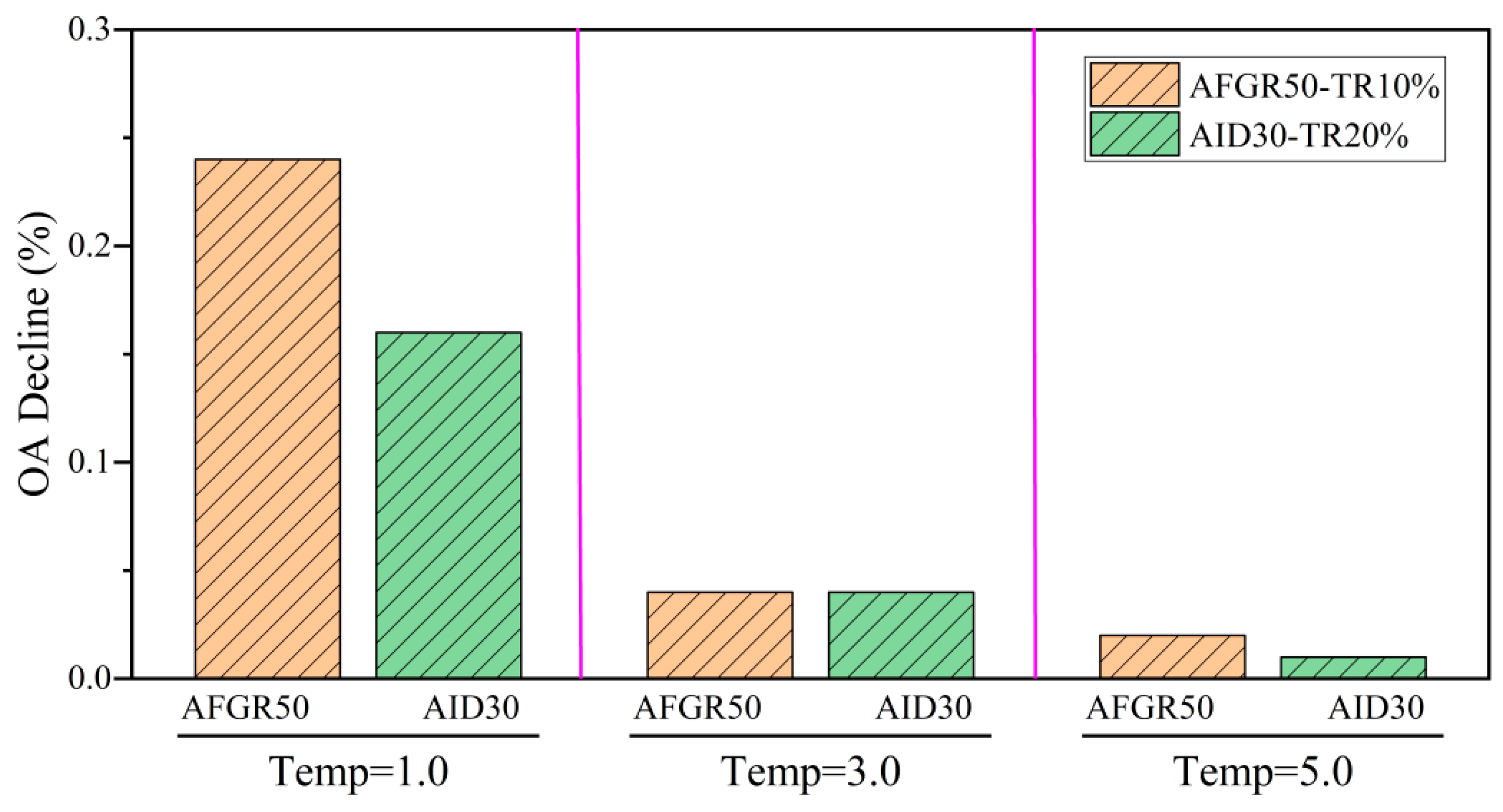
4.4.2. Sensitivity of Distillation Temperature

Figure 9 (shown below) illustrates how variations in the temperature parameter affect OA values during the KD processes, with 2.0 serving as the optimal reference temperature established in our experiments. At a temperature of 1.0, both the AFGR50-TR10% and AID30-TR20% configurations exhibit noticeable OA reductions, exceeding 0.2% and approximately 0.15%, respectively. Increasing the temperature to 3.0 substantially alleviates these declines, with accuracy reductions dropping below 0.05% for both datasets, indicating enhanced stability. Further raising of the temperature to 5.0 results in only marginal improvements, with OA declines diminishing to nearly negligible levels around 0.02%. These results highlight that a moderate temperature, particularly near 2.0, strikes an effective balance between soft target informativeness and gradient scale, thereby enabling efficient knowledge distillation with minimal accuracy loss.

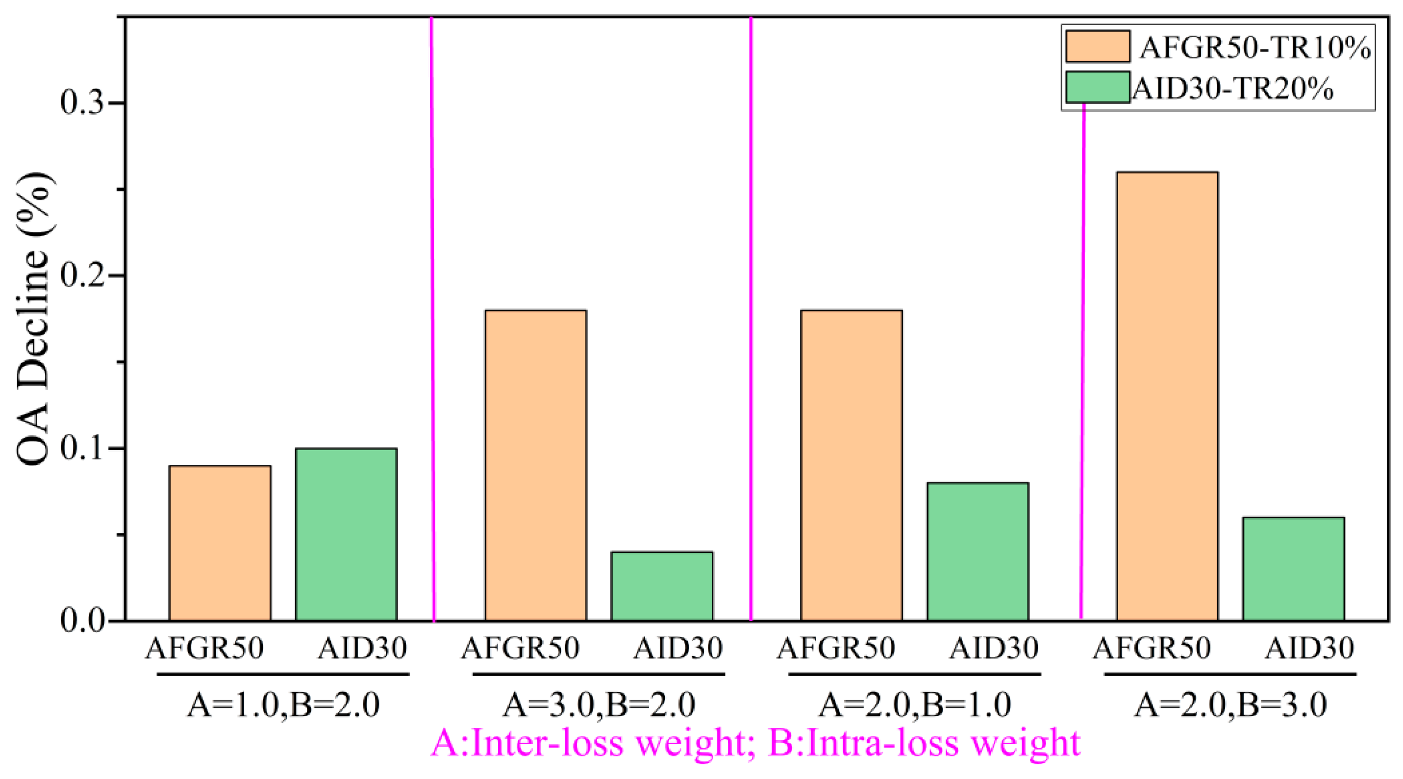
4.4.3. Sensitivity of Weights for Inter- and Intra-Loss

Figure 10 illustrates the OA declines observed when inter-loss (A) and intra-loss (B) weights deviate from the optimal configuration of A = 2.0 and B = 2.0. Reducing A to 1.0 or increasing it to 3.0 (with B fixed at 2.0) results in OA declines of approximately 0.09% and 0.17% for AFGR50-TR10% and 0.1% and 0.05% for AID30-TR20%, respectively. Similarly, altering B while keeping A at 2.0 shows that B = 1.0 produces comparable declines with high A settings, while B = 3.0 leads to the largest OA drop for AFGR50-TR10% (over 0.27%), with minimal effect on AID30-TR20% (around 0.05%). These results highlight the importance of balanced loss weights for ensuring robust distillation performance with minimal accuracy degradation, consistent with recommendations in the literature [84].

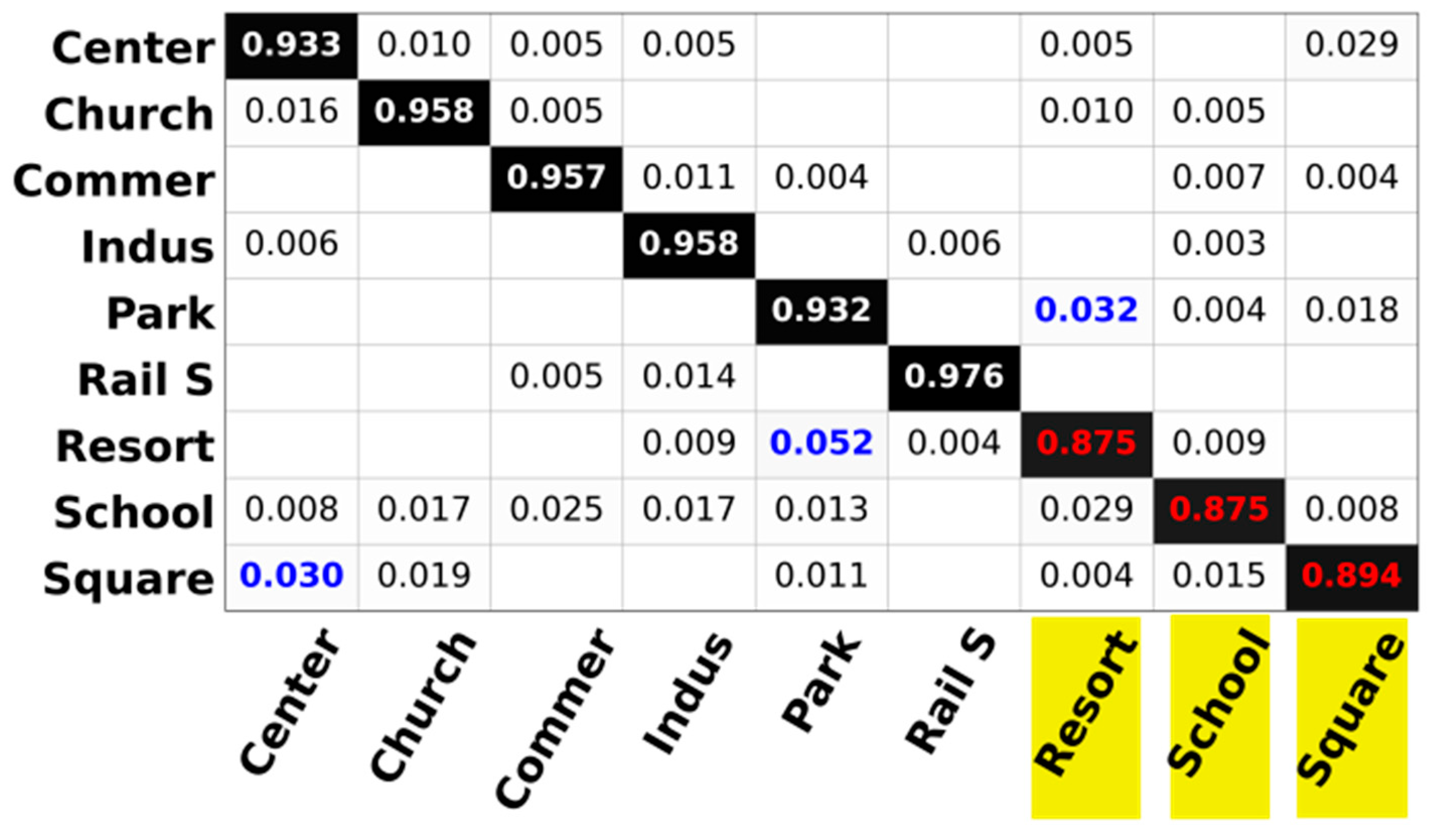
4.5. Confusion Matrix

Figure 11, Figure 12 and Figure 13 display the confusion matrices of our student-B1 model for the AID30, AFGR50, and NWPU45 datasets, respectively. Each figure shares a TR of 20%, facilitating the comparison of recognition challenges across the three datasets. An OA of 100% is represented as 1.0, and categories with an OA exceeding 98% are excluded from all figures. Values highlighted in blue indicate a misclassification ratio above 3%, while those in red, along with their category names marked in yellow, signify an OA below 93%.

Figure 11 indicates that the most challenging categories within the AID30 dataset are the resort, school, and square classes. The resort and square classes exhibit significant similarity to the park and center classes, respectively. Furthermore, nine categories have an OA below 98%, suggesting that approximately one-third of the classes within AID30 exhibit intra-class similarity. The resort and school classes have sample sizes of 290 and 300, respectively, which are below the average for all categories. Consequently, when using a larger TR as a performance indicator for the AID30 dataset, the impact on accuracy from the random selection of training samples becomes more pronounced.

Figure 12 shows that the most challenging categories within the AFGR50 dataset include five classes: A17, A31, A33, A39, and A46. The inter-class similarities within AFGR50 are greater than those within AID30. Specifically, twenty-three categories have an OA below 98%, indicating that about half of the classes within AFGR50 exhibit intra-class similarity. Moreover, categories with a higher misclassification ratio within AFGR50 are more dispersed than those within AID30. The lowest accuracy for all categories within AFGR50 is approximately 7% less than that within AID30. These observations confirm that classifying the AFGR50 dataset is more challenging compared with the AID30 dataset.

Figure 13 illustrates that 26 out of the 45 classes within the NWPU45 dataset have an OA below 98%, signifying a higher number of challenging categories compared with the AFGR50 dataset. The most difficult classes, with an OA falling below 93%, include the church, medium residential, palace, and rectangular farmland. Notably, the church and palace classes demonstrate significant misclassification ratios, peaking at 12.3% and 7.5%, respectively, largely due to mutual misclassification. These findings emphasize the intricacy of these classes within the NWPU45 dataset.

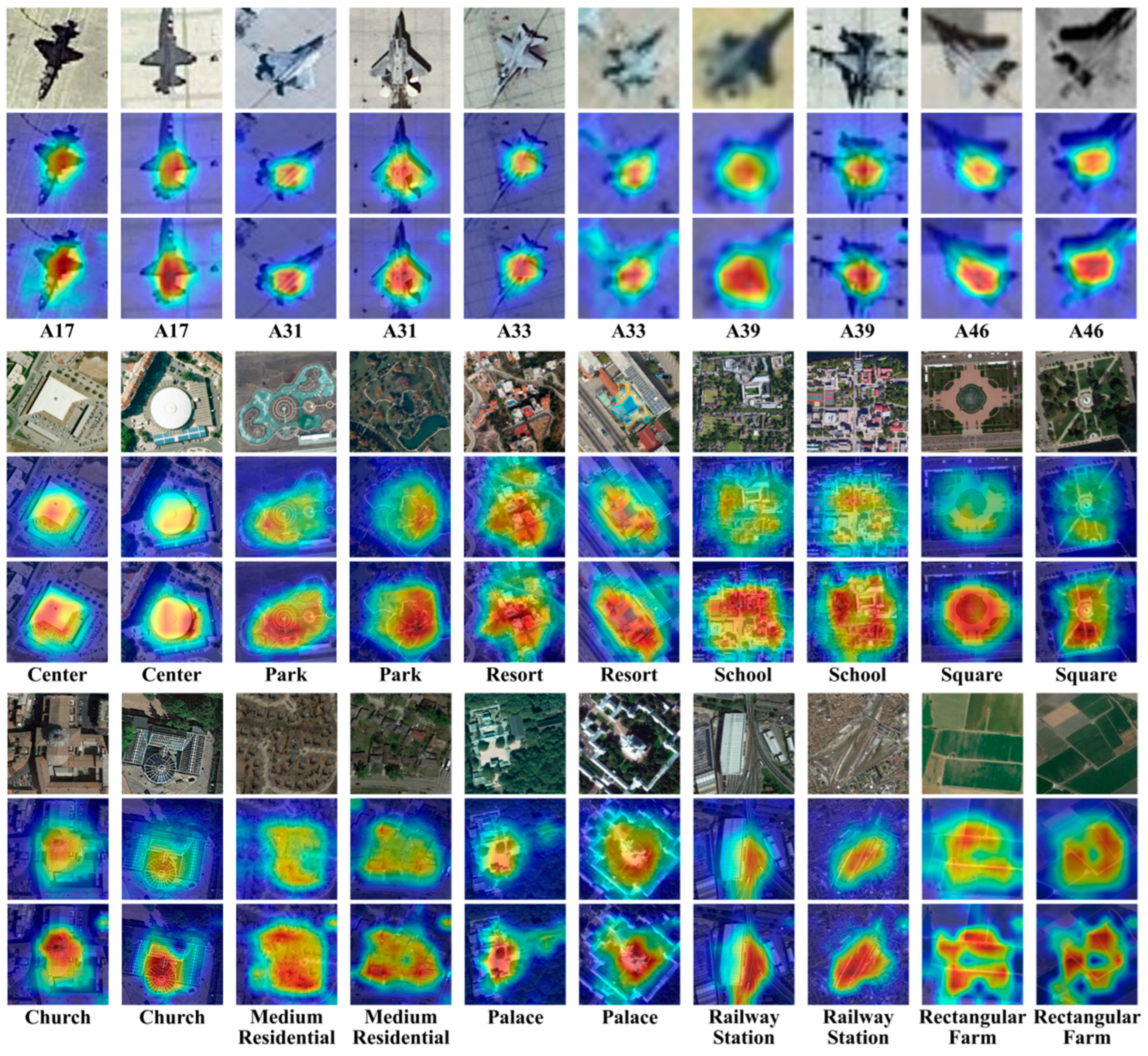
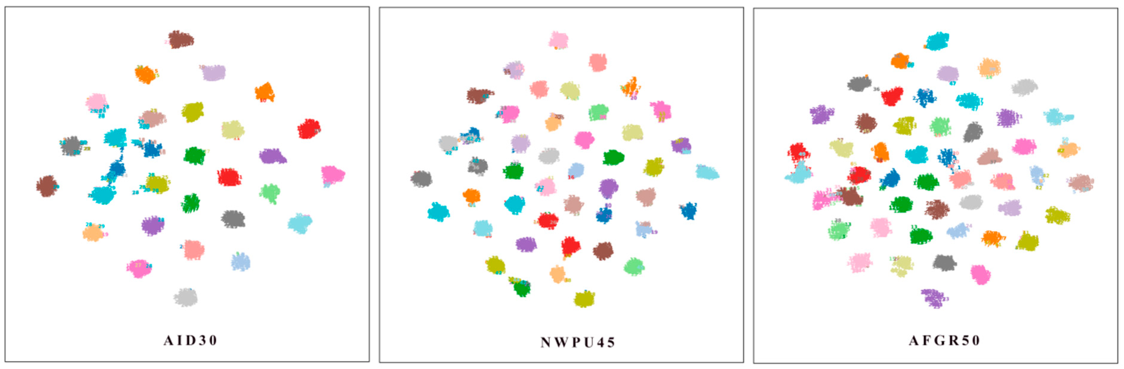
4.6. Visualization and Analysis

Figure 14 (shown below) illustrates the decision-making processes of the student-B1 model and its teacher using gradient-weighted class activation mapping (Grad-CAM). It is organized into three panels, each corresponding to the AFGR50, AID30, and NWPU45 datasets. For each panel, the top row shows original samples, while the second and third rows display the teacher’s and student-B1’s class activation maps, respectively, focusing on categories with lower accuracy.

In these maps, brighter regions denote the discriminative features that most strongly influence the model’s predictions. The close alignment of attention—such as aircraft wings in AFGR50, key ground targets in AID30, and roof structures in NWPU45—confirms consistent decision patterns and enhances interpretability. In classes with high intra-class similarity (e.g., schools or residential areas), both models attend to broader regions of the image. These findings demonstrate that student-B1 effectively inherits the teacher’s reasoning patterns, thereby improving transparency in the distillation process.

Figure 15 provides a visual demonstration of the feature effectiveness of our student-B1 model, using a technique known as t-distributed stochastic neighbor embedding (t-SNE). This technique projects model features onto a two-dimensional map, and the spatial distances between different category clusters on this map are used as indicators to measure feature effectiveness. The figure contains three separate subplots, each corresponding to a 20% TR on the AID30, NWPU45, and AFGR50 datasets.

Figure 15 presents t-SNE visualizations of the features extracted by student-B1, where pronounced inter-cluster distances attest to their discriminative power. The AID30 map shows the clearest separation—likely a result of its higher image resolution—while the AFGR50 and NWPU45 maps exhibit tighter clusters, reflecting their larger category sets and the model’s lower overall accuracies on those datasets. Overlapping clusters correspond to the challenging categories identified in the confusion matrices. Nevertheless, the high precision values reported in Section 4.3.3 confirm minimal false positives, underscoring the model’s robustness. Collectively, these t-SNE results validate the effectiveness of student-B1’s learned features.

4.7. Evaluation of Computational Efficiency

Table 14. Comparative analysis of computational efficiency among different methods.

Method	Params (M)	FLOPs (G)	Inferring Time (second)
P2FEViT [77]	>112.2	>21.7	73.39 ± 0.21
TST-Net [82]	173.0	30.2	150.39 ± 0.04
EfficientNet-B3	12.2	1.8	23.80 ± 0.02
ResNet-50	25.2	4.1	23.78 ± 0.01
Swin Transformer-tiny	28.3	4.5	31.98 ± 0.23
Swin Transformer-base	87.8	20.3	75.64 ± 0.10
Teacher Ensemble (heavy)	48.7	6.9	71.85 ± 0.01
Teacher Ensemble	32.7	4.3	50.79 ± 0.07
Student ResNet-18	11.7	1.8	11.63 ± 0.01
Student MobileNet-V2	3.5	0.3	11.69 ± 0.01
Student-B0	5.3	0.4	12.70 ± 0.07
Student-B1	7.8	0.7	17.43 ± 0.01

offers a comparative study of the computational efficiency of our models against two other leading multi-model methods documented in the literature: P2FEViT [77] and TS-TNet [82]. The replication of these two methods is based on their foundational models, given the absence of codes for other functional modules in the cited references. As a result, the inference speeds we have evaluated for these methods are, in theory, faster than their actual speeds.

Given the significant impact of operation parameter types on the inference speeds of models, we have chosen to use practical inference efficiency on GPUs as our performance indicators. The experiments consist of prediction processes for 25,200 RSI samples at a resolution of 256². The test environment, which is identical to the one previously described, utilizes a single RTX-4070Ti GPU. Additionally, the quantity of floating-point operations (FLOPs) is gauged in giga (G) units.

The table’s information demonstrates that our teacher model has achieved a 23% reduction in time costs for the proposed test, compared with the widely used Swin Transformer-base model. Simultaneously, our student-B1 model has shown a significant time saving of 66% in comparison with its teacher model. When our student-B1 model is compared with the multi-model methods of P2FEViT and TS-TNet, it exhibits superior performance with a reduction in time costs of 66% and 88% and a decrease in model sizes of 93% and 96%, respectively. Moreover, our student-B1 model has displayed a stronger generalization capability, outperforming P2FEViT on the fine-grained AFGR50 dataset. These findings highlight the proficiency of our method in generating solutions for RSI classification that are both accurate and lightweight.

5. Discussion

While this research presents a novel and effective solution for enhancing KD techniques in RSI classification, it is not without its limitations.

First, while the proposed symmetry-aware KD method significantly improves performance by addressing data asymmetry, it relies heavily on the quality of the training data. If the dataset is inherently noisy or contains substantial imbalances beyond the typical sparse distribution, the effectiveness of the symmetry-enhanced augmentation may be reduced. Furthermore, while the approach demonstrates remarkable reductions in model size and inference time, its generalizability across diverse remote sensing environments and varying hardware configurations remains to be thoroughly explored. Another limitation lies in the reliance on the logit-based KD process, which, while effective in this context, may not be universally applicable to all types of models or datasets.

Additionally, while our method requires no architectural changes, its performance gains might be contingent on specific properties of the datasets used in the experiments. As such, further investigation into how the method adapts to different remote sensing tasks and its scalability across large-scale deployments is needed. Finally, although the focus on symmetry preservation and data-driven solutions is a strength, the method could be further enhanced by integrating more advanced model optimization techniques to complement the data augmentation and feature alignment processes, thereby pushing the boundaries of lightweight model development.

6. Conclusions

This paper introduces a novel, data-driven approach to enhance the logit-based KD process for RSI classification. Our method is characterized by four innovations: a symmetry-aware strategy for solving the asymmetry in RSI samples, an ensemble generation algorithm for lightweight CNN models, a quantitative feature alignment technique, and integration into the SLT module.

Our key contributions are threefold. First, we address the challenge of asymmetries in RSI samples, proposing the SLT strategy to preserve symmetry and improve KD efficiency. Second, our method outperforms existing KD-based and other advanced techniques in RSI classification, offering superior accuracy. Lastly, our symmetry-aware approach, requiring no architectural modifications, provides an efficient solution for lightweight and accurate RSI classifiers. Evaluations on three benchmark datasets show that our student model surpasses 14 KD-based methods and 30 other advanced approaches, achieving better accuracy, reduced model size (up to 96%), and faster inference (up to 88%).

In conclusion, our method makes a significant contribution to RSI classification by offering a symmetry-driven, efficient approach to KD. Future work should explore the generalization of the proposed method to other datasets, real-world applications, and deployment on mobile and embedded devices to further enhance its robustness, scalability, and practical utility.

References

1. Lenton, T.M.; Abrams, J.F.; Bartsch, A.; Bathiany, S.; Boulton, C.A.; Buxton, J.E.; Conversi, A.; Cunliffe, A.M.; Hebden, S.; Lavergne, T.; et al. Remotely sensing potential climate change tipping points across scales. Nat. Commun. 2024, 15, 343. [Google Scholar] [CrossRef] [PubMed]
2. Lara-Alvarez, C.; Flores, J.J.; Rodriguez-Rangel, H.; Lopez-Farias, R. A literature review on satellite image time series forecasting: Methods and applications for remote sensing. WIREs Data Min. Knowl. Discov. 2024, 14, e1528. [Google Scholar] [CrossRef]
3. Dong, X.; Cao, J.; Zhao, W. A review of research on remote sensing images shadow detection and application to building extraction. Eur. J. Remote Sens. 2024, 57, 2293163. [Google Scholar] [CrossRef]
4. Vasquez, J.; Acevedo-Barrios, R.; Miranda-Castro, W.; Guerrero, M.; Meneses-Ospina, L. Determining Changes in Mangrove Cover Using Remote Sensing with Landsat Images: A Review. Water Air Soil Pollut. 2023, 235, 18. [Google Scholar] [CrossRef]
5. Dutta, S.; Das, M. Remote sensing scene classification under scarcity of labelled samples—A survey of the state-of-the-arts. Comput. Geosci. 2023, 171, 105295. [Google Scholar] [CrossRef]
6. Adegun, A.A.; Viriri, S.; Tapamo, J.-R. Review of deep learning methods for remote sensing satellite images classification: Experimental survey and comparative analysis. J. Big Data 2023, 10, 93. [Google Scholar] [CrossRef]
7. Chong, Q.; Ni, M.; Huang, J.; Wei, G.; Li, Z.; Xu, J. Rethinking high-resolution remote sensing image segmentation not limited to technology: A review of segmentation methods and outlook on technical interpretability. Int. J. Remote Sens. 2024, 45, 3689–3716. [Google Scholar] [CrossRef]
8. Zhao, H.; Morgenroth, J.; Pearse, G.; Schindler, J. A Systematic Review of Individual Tree Crown Detection and Delineation with Convolutional Neural Networks (CNN). Curr. For. Rep. 2023, 9, 149–170. [Google Scholar] [CrossRef]
9. Xu, T.; Zhao, Z.; Wu, J. Breaking the ImageNet Pretraining Paradigm: A General Framework for Training Using Only Remote Sensing Scene Images. Appl. Sci. 2023, 13, 11374. [Google Scholar] [CrossRef]
10. Ma, Y.; Meng, J.; Liu, B.; Sun, L.; Zhang, H.; Ren, P. Dictionary Learning for Few-Shot Remote Sensing Scene Classification. Remote Sens. 2023, 15, 773. [Google Scholar] [CrossRef]
11. Zhou, Z.; Li, S.; Wu, W.; Guo, W.; Li, X.; Xia, G.; Zhao, Z. NaSC-TG2: Natural Scene Classification with Tiangong-2 Remotely Sensed Imagery. IEEE J. Sel. Top. Appl. Earth Obs. Remote Sens. 2021, 14, 3228–3242. [Google Scholar] [CrossRef]
12. Han, K.; Wang, Y.; Chen, H.; Chen, X.; Guo, J.; Liu, Z.; Tang, Y.; Xiao, A.; Xu, C.; Xu, Y.; et al. A Survey on Vision Transformer. IEEE Trans. Pattern Anal. Mach. Intell. 2023, 45, 87–110. [Google Scholar] [CrossRef] [PubMed]
13. Kumari, M.; Kaul, A. Recent advances in the application of vision transformers to remote sensing image scene classification. Remote Sens. Lett. 2023, 14, 722–732. [Google Scholar] [CrossRef]
14. Fayad, I.; Ciais, P.; Schwartz, M.; Wigneron, J.-P.; Baghdadi, N.; de Truchis, A.; D’ASpremont, A.; Frappart, F.; Saatchi, S.; Sean, E.; et al. Hy-TeC: A hybrid vision transformer model for high-resolution and large-scale mapping of canopy height. Remote Sens. Environ. 2024, 302, 113945. [Google Scholar] [CrossRef]
15. Song, H. MBC-Net: Long-range enhanced feature fusion for classifying remote sensing images. Int. J. Intell. Comput. Cybern. 2024, 17, 181–209. [Google Scholar] [CrossRef]
16. Song, H.; Yuan, Y.; Ouyang, Z.; Yang, Y.; Xiang, H. Quantitative regularization in robust vision transformer for remote sensing image classification. Photogramm. Rec. 2024, 39, 340–372. [Google Scholar] [CrossRef]
17. Song, H.; Xia, H.; Wang, W.; Zhou, Y.; Liu, W.; Liu, Q.; Liu, J. QAGA-Net: Enhanced vision transformer-based object detection for remote sensing images. Int. J. Intell. Comput. Cybern. 2025, 18, 133–152. [Google Scholar] [CrossRef]
18. Song, H.; Xie, J.; Wang, Y.; Fu, L.; Zhou, Y.; Zhou, X. Optimized Data Distribution Learning for Enhancing Vision Transformer-Based Object Detection in Remote Sensing Images. Photogramm. Rec. 2025, 40, e70004. [Google Scholar] [CrossRef]
19. Cao, Z.; Kooistra, L.; Wang, W.; Guo, L.; Valente, J. Real-Time Object Detection Based on UAV Remote Sensing: A Systematic Literature Review. Drones 2023, 7, 620. [Google Scholar] [CrossRef]
20. Tang, W.; He, F.; Bashir, A.K.; Shao, X.; Cheng, Y.; Yu, K. A remote sensing image rotation object detection approach for real-time environmental monitoring. Sustain. Energy Technol. Assess. 2023, 57, 103270. [Google Scholar] [CrossRef]
21. Pal, M. Deep learning algorithms for hyperspectral remote sensing classifications: An applied review. Int. J. Remote Sens. 2024, 45, 451–491. [Google Scholar] [CrossRef]
22. Wang, R.; Ma, L.; He, G.; Johnson, B.A.; Yan, Z.; Chang, M.; Liang, Y. Transformers for Remote Sensing: A Systematic Review and Analysis. Sensors 2024, 24, 3495. [Google Scholar] [CrossRef] [PubMed]
23. Thapa, A.; Horanont, T.; Neupane, B.; Aryal, J. Deep Learning for Remote Sensing Image Scene Classification: A Review and Meta-Analysis. Remote Sens. 2023, 15, 4804. [Google Scholar] [CrossRef]
24. Song, H.; Xie, H.; Duan, Y.; Xie, X.; Gan, F.; Wang, W.; Liu, J. Pure data correction enhancing remote sensing image classification with a lightweight ensemble model. Sci. Rep. 2025, 15, 5507. [Google Scholar] [CrossRef]
25. Lee, G.Y.; Dam, T.; Ferdaus, M.M.; Poenar, D.P.; Duong, V.N. Unlocking the capabilities of explainable few-shot learning in remote sensing. Artif. Intell. Rev. 2024, 57, 169. [Google Scholar] [CrossRef]
26. Chen, Z.; Zhang, C.; Zhang, B.; He, Y. Triplet Contrastive Learning Framework with Adversarial Hard-Negative Sample Generation for Multimodal Remote Sensing Images. IEEE Trans. Geosci. Remote Sens. 2024, 62, 5506015. [Google Scholar] [CrossRef]
27. Liu, Y.; Liu, S.; Li, T.; Li, T.; Li, W.; Wang, G.; Liu, X.; Yang, W.; Liu, Y. Towards constructing a DOE-based practical optical neural system for ship recognition in remote sensing images. Signal Process. 2024, 221, 109488. [Google Scholar] [CrossRef]
28. Jin, E.; Du, J.; Bi, Y.; Wang, S.; Gao, X. Research on Classification of Grassland Degeneration Indicator Objects Based on UAV Hyperspectral Remote Sensing and 3D_RNet-O Model. Sensors 2024, 24, 1114. [Google Scholar] [CrossRef]
29. Zhang, R.; Jin, S.; Zhang, Y.; Zang, J.; Wang, Y.; Li, Q.; Sun, Z.; Wang, X.; Zhou, Q.; Cai, J.; et al. PhenoNet: A two-stage lightweight deep learning framework for real-time wheat phenophase classification. ISPRS J. Photogramm. Remote Sens. 2024, 208, 136–157. [Google Scholar] [CrossRef]
30. Zheng, Y.-J.; Chen, S.-B.; Ding, C.H.Q.; Luo, B. Model Compression Based on Differentiable Network Channel Pruning. IEEE Trans. Neural Netw. Learn. Syst. 2023, 34, 10203–10212. [Google Scholar] [CrossRef]
31. Rajpal, M.; Zhang, Y.; Low, B.K.H. Pruning during training by network efficacy modeling. Mach. Learn. 2023, 112, 2653–2684. [Google Scholar] [CrossRef]
32. Yuan, M.; Lang, B.; Quan, F. Student-friendly knowledge distillation. Knowl.-Based Syst. 2024, 296, 111915. [Google Scholar] [CrossRef]
33. Liu, Y.; Cao, J.; Li, B.; Hu, W.; Ding, J.; Li, L.; Maybank, S. Cross-Architecture Knowledge Distillation. Int. J. Comput. Vis. 2024, 132, 2798–2824. [Google Scholar] [CrossRef]
34. Song, H.; Yuan, Y.; Ouyang, Z.; Yang, Y.; Xiang, H. Efficient knowledge distillation for hybrid models: A vision transformer-convolutional neural network to convolutional neural network approach for classifying remote sensing images. IET Cyber-Syst. Robot. 2024, 6, e12120. [Google Scholar] [CrossRef]
35. Yue, H.; Li, J.; Liu, H. Second-Order Unsupervised Feature Selection via Knowledge Contrastive Distillation. IEEE Trans. Pattern Anal. Mach. Intell. 2023, 45, 15577–15587. [Google Scholar] [CrossRef]
36. Zheng, Z.; Ye, R.; Hou, Q.; Ren, D.; Wang, P.; Zuo, W.; Cheng, M.-M. Localization Distillation for Object Detection. IEEE Trans. Pattern Anal. Mach. Intell. 2023, 45, 10070–10083. [Google Scholar] [CrossRef]
37. Wang, J.; Zhang, W.; Guo, Y.; Liang, P.; Ji, M.; Zhen, C.; Wang, H. Global key knowledge distillation framework. Comput. Vis. Image Underst. 2024, 239, 103902. [Google Scholar] [CrossRef]
38. Tian, L.; Wang, Z.; He, B.; He, C.; Wang, D.; Li, D. Knowledge Distillation of Grassmann Manifold Network for Remote Sensing Scene Classification. Remote Sens. 2021, 13, 4537. [Google Scholar] [CrossRef]
39. Zhao, H.; Sun, X.; Gao, F.; Dong, J. Pair-Wise Similarity Knowledge Distillation for RSI Scene Classification. Remote Sens. 2022, 14, 2483. [Google Scholar] [CrossRef]
40. Xu, K.; Deng, P.; Huang, H. Vision Transformer: An Excellent Teacher for Guiding Small Networks in Remote Sensing Image Scene Classification. IEEE Trans. Geosci. Remote Sens. 2022, 60, 5618715. [Google Scholar] [CrossRef]
41. Li, D.; Nan, Y.; Liu, Y. Remote Sensing Image Scene Classification Model Based on Dual Knowledge Distillation. IEEE Geosci. Remote Sens. Lett. 2022, 19, 4514305. [Google Scholar] [CrossRef]
42. Zhang, N.; Wang, G.; Wang, J.; Chen, H.; Liu, W.; Chen, L. All Adder Neural Networks for On-Board Remote Sensing Scene Classification. IEEE Trans. Geosci. Remote Sens. 2023, 61, 5607916. [Google Scholar] [CrossRef]
43. Zhang, T.; Wang, Z.; Cheng, P.; Xu, G.; Sun, X. DCNNet: A Distributed Convolutional Neural Network for Remote Sensing Image Classification. IEEE Trans. Geosci. Remote Sens. 2023, 61, 5603618. [Google Scholar] [CrossRef]
44. Zhao, Y.; Liu, J.; Yang, J.; Wu, Z. EMSCNet: Efficient Multisample Contrastive Network for Remote Sensing Image Scene Classification. IEEE Trans. Geosci. Remote Sens. 2023, 61, 5605814. [Google Scholar] [CrossRef]
45. Xing, S.; Xing, J.; Ju, J.; Hou, Q.; Ding, X. Collaborative Consistent Knowledge Distillation Framework for Remote Sensing Image Scene Classification Network. Remote Sens. 2022, 14, 5186. [Google Scholar] [CrossRef]
46. Wang, X.; Zhu, J.; Yan, Z.; Zhang, Z.; Zhang, Y.; Chen, Y.; Li, H. LaST: Label-Free Self-Distillation Contrastive Learning with Transformer Architecture for Remote Sensing Image Scene Classification. IEEE Geosci. Remote Sens. Lett. 2022, 19, 6512205. [Google Scholar] [CrossRef]
47. Hu, Y.; Huang, X.; Luo, X.; Han, J.; Cao, X.; Zhang, J. Variational Self-Distillation for Remote Sensing Scene Classification. IEEE Trans. Geosci. Remote Sens. 2022, 60, 5627313. [Google Scholar] [CrossRef]
48. Zhao, Q.; Ma, Y.; Lyu, S.; Chen, L. Embedded Self-Distillation in Compact Multibranch Ensemble Network for Remote Sensing Scene Classification. IEEE Trans. Geosci. Remote Sens. 2022, 60, 4506415. [Google Scholar] [CrossRef]
49. Zhao, Y.; Liu, J.; Yang, J.; Wu, Z. Remote Sensing Image Scene Classification via Self-Supervised Learning and Knowledge Distillation. Remote Sens. 2022, 14, 4813. [Google Scholar] [CrossRef]
50. Shi, C.; Ding, M.; Wang, L.; Pan, H. Learn by Yourself: A Feature-Augmented Self-Distillation Convolutional Neural Network for Remote Sensing Scene Image Classification. Remote Sens. 2023, 15, 5620. [Google Scholar] [CrossRef]
51. Wu, B.; Hao, S.; Wang, W. Class-Aware Self-Distillation for Remote Sensing Image Scene Classification. IEEE J. Sel. Top. Appl. Earth Obs. Remote Sens. 2024, 17, 2173–2188. [Google Scholar] [CrossRef]
52. Xie, W.; Fan, X.; Zhang, X.; Li, Y.; Sheng, M.; Fang, L. Co-Compression via Superior Gene for Remote Sensing Scene Classification. IEEE Trans. Geosci. Remote Sens. 2023, 61, 5604112. [Google Scholar] [CrossRef]
53. Alhichri, H.; Alswayed, A.S.; Bazi, Y.; Ammour, N.; Alajlan, N.A. Classification of Remote Sensing Images Using EfficientNet-B3 CNN Model with Attention. IEEE Access 2021, 9, 14078–14094. [Google Scholar] [CrossRef]
54. Liang, L.; Wang, G. Efficient recurrent attention network for remote sensing scene classification. IET Image Process. 2021, 15, 1712–1721. [Google Scholar] [CrossRef]
55. Yang, S.; Song, F.; Jeon, G.; Sun, R. Scene Changes Understanding Framework Based on Graph Convolutional Networks and Swin Transformer Blocks for Monitoring LCLU Using High-Resolution Remote Sensing Images. Remote Sens. 2022, 14, 3709. [Google Scholar] [CrossRef]
56. Sinaga, K.B.M.; Yudistira, N.; Santoso, E. Efficient CNN for high-resolution remote sensing imagery understanding. Multimed. Tools Appl. 2023, 83, 61737–61759. [Google Scholar] [CrossRef]
57. Alharbi, R.; Alhichri, H.; Ouni, R.; Bazi, Y.; Alsabaan, M. Improving remote sensing scene classification using quality-based data augmentation. Int. J. Remote Sens. 2023, 44, 1749–1765. [Google Scholar] [CrossRef]
58. Zheng, F.; Lin, S.; Zhou, W.; Huang, H. A Lightweight Dual-Branch Swin Transformer for Remote Sensing Scene Classification. Remote Sens. 2023, 15, 2865. [Google Scholar] [CrossRef]
59. Song, J.; Fan, Y.; Song, W.; Zhou, H.; Yang, L.; Huang, Q.; Jiang, Z.; Wang, C.; Liao, T. SwinHCST: A deep learning network architecture for scene classification of remote sensing images based on improved CNN and Transformer. Int. J. Remote Sens. 2023, 44, 7439–7463. [Google Scholar] [CrossRef]
60. Chen, X.; Ma, M.; Li, Y.; Mei, S.; Han, Z.; Zhao, J.; Cheng, W. Hierarchical Feature Fusion of Transformer with Patch Dilating for Remote Sensing Scene Classification. IEEE Trans. Geosci. Remote Sens. 2023, 61, 4410516. [Google Scholar] [CrossRef]
61. Hao, S.; Li, N.; Ye, Y. Inductive Biased Swin-Transformer with Cyclic Regressor for Remote Sensing Scene Classification. IEEE J. Sel. Top. Appl. Earth Obs. Remote Sens. 2023, 16, 6265–6278. [Google Scholar] [CrossRef]
62. Wang, G.; Zhang, N.; Liu, W.; Chen, H.; Xie, Y. MFST: A Multi-Level Fusion Network for Remote Sensing Scene Classification. IEEE Geosci. Remote Sens. Lett. 2022, 19, 6516005. [Google Scholar] [CrossRef]
63. Zhou, M.; Zhou, Y.; Yang, D.; Song, K. Remote Sensing Image Classification Based on Canny Operator Enhanced Edge Features. Sensors 2024, 24, 3912. [Google Scholar] [CrossRef] [PubMed]
64. Hou, Y.-E.; Yang, K.; Dang, L.; Liu, Y. Contextual Spatial-Channel Attention Network for Remote Sensing Scene Classification. IEEE Geosci. Remote Sens. Lett. 2023, 20, 6008805. [Google Scholar] [CrossRef]
65. Li, D.; Liu, R.; Tang, Y.; Liu, Y. PSCLI-TF: Position-Sensitive Cross-Layer Interactive Transformer Model for Remote Sensing Image Scene Classification. IEEE Geosci. Remote Sens. Lett. 2024, 21, 5001305. [Google Scholar] [CrossRef]
66. Sitaula, C.; Kc, S.; Aryal, J. Enhanced multi-level features for very high resolution remote sensing scene classification. Neural Comput. Appl. 2024, 36, 7071–7083. [Google Scholar] [CrossRef]
67. Wang, W.; Sun, Y.; Li, J.; Wang, X. Frequency and spatial based multi-layer context network (FSCNet) for remote sensing scene classification. Int. J. Appl. Earth Obs. Geoinf. 2024, 128, 103781. [Google Scholar] [CrossRef]
68. Xia, J.; Zhou, Y.; Tan, L.; Ding, Y. MCAFNet: Multi-Channel Attention Fusion Network-Based CNN For Remote Sensing Scene Classification. Photogramm. Eng. Remote Sens. 2023, 89, 183–192. [Google Scholar] [CrossRef]
69. Chen, Z.; Yang, J.; Feng, Z.; Chen, L.; Li, L. BiShuffleNeXt: A lightweight bi-path network for remote sensing scene classification. Measurement 2023, 209, 112537. [Google Scholar] [CrossRef]
70. Sagar, A.S.M.S.; Tanveer, J.; Chen, Y.; Dang, L.M.; Haider, A.; Song, H.-K.; Moon, H. BayesNet: Enhancing UAV-Based Remote Sensing Scene Understanding with Quantifiable Uncertainties. Remote Sens. 2024, 16, 925. [Google Scholar] [CrossRef]
71. Albarakati, H.M.; Khan, M.A.; Hamza, A.; Khan, F.; Kraiem, N.; Jamel, L.; Almuqren, L.; Alroobaea, R. A Novel Deep Learning Architecture for Agriculture Land Cover and Land Use Classification from Remote Sensing Images Based on Network-Level Fusion of Self-Attention Architecture. IEEE J. Sel. Top. Appl. Earth Obs. Remote Sens. 2024, 17, 6338–6353. [Google Scholar] [CrossRef]
72. Shi, C.; Zhang, X.; Wang, L.; Jin, Z. A lightweight convolution neural network based on joint features for Remote Sensing scene image classification. Int. J. Remote Sens. 2023, 44, 6615–6641. [Google Scholar] [CrossRef]
73. Shen, X.; Wang, H.; Wei, B.; Cao, J. Real-time scene classification of unmanned aerial vehicles remote sensing image based on Modified GhostNet. PLoS ONE 2023, 18, e0286873. [Google Scholar] [CrossRef]
74. Bi, M.; Wang, M.; Li, Z.; Hong, D. Vision Transformer with Contrastive Learning for Remote Sensing Image Scene Classification. IEEE J. Sel. Top. Appl. Earth Obs. Remote Sens. 2023, 16, 738–749. [Google Scholar] [CrossRef]
75. Lu, W.; Chen, S.-B.; Tang, J.; Ding, C.H.Q.; Luo, B. A Robust Feature Downsampling Module for Remote-Sensing Visual Tasks. IEEE Trans. Geosci. Remote Sens. 2023, 61, 4404312. [Google Scholar] [CrossRef]
76. Zhao, M.; Meng, Q.; Zhang, L.; Hu, X.; Bruzzone, L. Local and Long-Range Collaborative Learning for Remote Sensing Scene Classification. IEEE Trans. Geosci. Remote Sens. 2023, 61, 5606215. [Google Scholar] [CrossRef]
77. Wang, G.; Chen, H.; Chen, L.; Zhuang, Y.; Zhang, S.; Zhang, T.; Dong, H.; Gao, P. P2FEViT: Plug-and-Play CNN Feature Embedded Hybrid Vision Transformer for Remote Sensing Image Classification. Remote Sens. 2023, 15, 1773. [Google Scholar] [CrossRef]
78. Yue, H.; Qing, L.; Zhang, Z.; Wang, Z.; Guo, L.; Peng, Y. MSE-Net: A novel master–slave encoding network for remote sensing scene classification. Eng. Appl. Artif. Intell. 2024, 132, 107909. [Google Scholar] [CrossRef]
79. Yang, Y.; Jiao, L.; Liu, F.; Liu, X.; Li, L.; Chen, P.; Yang, S. An Explainable Spatial–Frequency Multiscale Transformer for Remote Sensing Scene Classification. IEEE Trans. Geosci. Remote Sens. 2023, 61, 5907515. [Google Scholar] [CrossRef]
80. Siddiqui, M.I.; Khan, K.; Fazil, A.; Zakwan, M. Snapshot ensemble-based residual network (SnapEnsemResNet) for remote sensing image scene classification. Geoinformatica 2023, 27, 341–372. [Google Scholar] [CrossRef]
81. Xiao, F.; Li, X.; Li, W.; Shi, J.; Zhang, N.; Gao, X. Integrating category-related key regions with a dual-stream network for remote sensing scene classification. J. Vis. Commun. Image Represent. 2024, 100, 104098. [Google Scholar] [CrossRef]
82. Hao, S.; Wu, B.; Zhao, K.; Ye, Y.; Wang, W. Two-Stream Swin Transformer with Differentiable Sobel Operator for Remote Sensing Image Classification. Remote Sens. 2022, 14, 1507. [Google Scholar] [CrossRef]
83. Stanton, S.; Izmailov, P.; Kirichenko, P.; Alemi, A.A.; Wilson, A.G. Does Knowledge Distillation Really Work? In Advances in Neural Information Processing Systems; Ranzato, M., Beygelzimer, A., Dauphin, Y., Liang, P.S., Vaughan, J.W., Eds.; Curran Associates, Inc.: Red Hook, NY, USA, 2021; pp. 6906–6919. Available online: https://proceedings.neurips.cc/paper_files/paper/2021/file/376c6b9ff3bedbbea56751a84fffc10c-Paper.pdf (accessed on 1 March 2025).
84. Huang, T.; You, S.; Wang, F.; Qian, C.; Xu, C. Knowledge Distillation from A Stronger Teacher. In Advances in Neural Information Processing Systems; Koyejo, S., Mohamed, S., Agarwal, A., Belgrave, D., Cho, K., Oh, A., Eds.; Curran Associates, Inc.: Red Hook, NY, USA, 2022; pp. 33716–33727. Available online: https://proceedings.neurips.cc/paper_files/paper/2022/file/da669dfd3c36c93905a17ddba01eef06-Paper-Conference.pdf (accessed on 1 March 2025).
85. Yun, S.; Han, D.; Chun, S.; Oh, S.J.; Yoo, Y.; Choe, J. CutMix: Regularization Strategy to Train Strong Classifiers with Localizable Features. In Proceedings of the 2019 IEEE/CVF International Conference on Computer Vision (ICCV), Seoul, Republic of Korea, 27 October–2 November 2019; pp. 6022–6031. [Google Scholar] [CrossRef]
86. Beyer, L.; Zhai, X.; Royer, A.; Markeeva, L.; Anil, R.; Kolesnikov, A. Knowledge distillation: A good teacher is patient and consistent. In Proceedings of the 2022 IEEE/CVF Conference on Computer Vision and Pattern Recognition (CVPR), New Orleans, LA, USA, 18–24 June 2022; IEEE: Piscataway, NJ, USA, 2022; pp. 10915–10924. [Google Scholar] [CrossRef]
Figure 1. A contrastive study of object representation in natural and remote sensing imagery.
Symmetry 17 01002 g001
Figure 2. Impact of sunlight and sensor focus on RSI quality.
Symmetry 17 01002 g002
Figure 3. The impact of variance within training data on function approximation.
Symmetry 17 01002 g003
Figure 4. Workflow of the proposed research work.
Symmetry 17 01002 g004
Figure 5. Algorithmic diagram of the proposed qualitative feature alignment technique.
Symmetry 17 01002 g005
Figure 6. Architecture of the teacher ensemble.
Symmetry 17 01002 g006
Figure 7. Framework of the proposed knowledge transferring process.
Symmetry 17 01002 g007
Figure 8. Difference between precision and OA of student-B1 across datasets.
Symmetry 17 01002 g008
Figure 9. Impact of temperature parameter on OA decline during KD processes.
Symmetry 17 01002 g009
Figure 10. Impact of inter- and intra-loss weights on OA decline in KD processes.
Symmetry 17 01002 g010
Figure 11. Confusion matrix for the AID30 dataset at a TR of 20%.
Symmetry 17 01002 g011
Figure 12. Confusion matrix for the AFGR50 dataset with a TR of 20%.
Symmetry 17 01002 g012
Figure 13. Confusion matrix for the NWPU45 dataset with a TR of 20%.
Symmetry 17 01002 g013
Figure 14. Grad-CAM analysis for model decision patterns.
Symmetry 17 01002 g014
Figure 15. t-SNE visualizations for the ADI30, NWPU45, and AFGR50 datasets.
Symmetry 17 01002 g015