Novel Methods for Multi-Switch Generalized Projective Anti-Synchronization of Fractional Chaotic System Under Caputo–Fabrizio Derivative via Lyapunov Stability Theorem and Adaptive Control

Abstract

The issue of multi-switch generalized projective anti-synchronization of fractional-order chaotic systems is investigated in this work. The model is constructed using Caputo–Fabrizio derivatives, which have been rarely addressed in previous research. In order to expand the symmetric and asymmetric synchronization modes of chaotic systems, we consider modeling chaotic systems under such fractional calculus definitions. Firstly, a new fractional-order differential inequality is proven, which facilitates the rapid confirmation of a suitable Lyapunov function. Secondly, an effective multi-switching controller is designed to confirm the convergence of the error system within a short moment to achieve synchronization asymptotically. Simultaneously, a multi-switching parameter adaptive principle is developed to appraise the uncertain parameters in the system. Finally, two simulation examples are presented to affirm the correctness and superiority of the introduced approach. It can be said that the symmetric properties of Caputo–Fabrizio fractional derivative are making outstanding contributions to the research on chaos synchronization.

1. Introduction

Fractional calculus is not an unfamiliar term to most people, and it has been over several centuries since its inception, largely owing to the significant contributions made by Newton and Leibniz in this field. Initially, it was primarily utilized for its theoretical value, but in recent decades, it has been endowed with characteristics such as memory and genetic properties [1]. As a result, it has found widespread application in various research areas, including physics [2], control engineering [3], biology [4], electrolytes [5], and dielectric polarization [6]. This is because the current state of a system described by fractional calculus depends on all of its previous states and, in turn, exerts an influence on the system’s future state. This property has been extensively applied by scientists across multiple disciplines.

The chaos phenomenon is a common and fundamental characteristic shared by most nonlinear systems. The term originates from the butterfly effect proposed by Lorentz in atmospheric science, which describes the potential for small changes in the initial conditions of nonlinear systems to cause significant deviations in the system’s future state. This unpredictability is generally undesirable for most researchers, and as a result, chaos synchronization and control have become key areas of focus. Since the concept of chaos synchronization was first introduced by Pecola in the 1990s [7], research in this field has steadily progressed and evolved, leading to the development of numerous effective synchronization methods, including complete synchronization [8], phase synchronization [9], sliding mode synchronization [10], projective synchronization [11], and combination synchronization [12]. The use of fractional calculus to describe chaos synchronization has emerged as a major trend in the study of nonlinear systems, and several high-quality articles in this area warrant further discussion. The characteristic function method is used to modify the adaptive filtering paradigm, and when combined with the fractional calculus method, a new filtering structure is constructed [13]. The one-dimensional adaptive synchronization strategy is used to discuss the status of fractional chaotic systems corresponding to the primordial Chua circuit, where chaotic behavior is generated by fractional-order systems with boundaries [14]. The Lyapunov method and fractional-order stability theory are used to derive adequate requirements for achieving asymptotic steadiness in a class of time fractional-order reaction–diffusion systems [15]. Particle swarm optimization and whale sequential minimal optimization are used to study the complete synchronization of several uniform fractional financial systems under various initial conditions. The considered chaotic system is highly dependent on parameter perturbations and initial conditions. Sensitivity analysis proves the rationality of the outcome of evidence [16]. The dynamic behavior of a new type of third-order nonlinear chaotic system was studied using the Lyapunov stability theorem. Under this condition, the system transitions from a chaotic condition to an erratic trivial fixed point [17]. The authors proposed dynamic coupling as a synchronization policy for fractional order chaotic systems. In their study, the integral order was considered to have a significant impact on the synchronization state, achieving complete synchronization of a number of systems [18]. Considering the constraints of the controller and the soft variable structure method, a finite time generalized projection control function was designed to address the limited time projection synchronization issue of two chaotic systems with operation restriction [19]. On account of the changeable order control strategy, sliding mode command technology is used to study the terminate time projection synchronization problem of two types of variable order chaotic systems [20]. In view of the stability theory proposed by Lyapunov of integer-order mapping and linear fractional order mapping, the full state mixed projection synchronization of the slave system and master system has been achieved. In their research, the system has both noninteger and integer order, filling some gaps in the above research [21].

Although the research mentioned above was conducted within the context of fractional calculus and various synchronization strategies were designed, all of these studies share a common characteristic: The system parameters are assumed to be known, which represents an idealized situation. However, in practical scenarios, the parameters of most nonlinear systems are unknown, and there are often external and nonlinear disturbances present, which complicate the control of the system. Despite these challenges, some researchers continue to take on these difficulties and engage in extensive and valuable research in this area. A new adaptive synchronization scheme with unidentified arguments was proposed on the basis of the stability theory of complex valued systems and complex variable inequalities, achieving synchronization of noninteger complex variable systems with unsuspected arguments [22]. On the basis of Ref. [22], the authors of Ref. [23] considered the complex correction projection synchronization problem of fractional-order complex variable chaotic systems with unknown complex parameters, effectively reducing the complexity of calculation and analysis in Ref. [22]. Sliding mode control technology was used to improve a class of adaptive sliding mode controllers and parameter update rates, achieving synchronization of two types of fractional-order chaotic systems with completely unknown parameters [24]. In Ref. [25], the authors used the Lyapunov stability theorem and appropriate adaptive control functions to realize dual synchronization of four hyperchaotic systems, which means that the adaptive parameter update rate has been extended to the synchronization between multiple systems. A new adaptive control method was designed using sliding mode control to achieve a synchronous driving response of two six-dimensional systems in the existence of exterior interference, parameter interference, and equivocal parameters [26]. In Ref. [27], the author studied the combination synchronization problem between four different systems using sliding mode control and adaptive control. The system parameters and disturbance upper bounds are completely unknown. Compared to previous studies, the difference lies in the limitations of Ref. [25] and the number of systems in Ref. [26], which have broader research significance. In most synchronization error states, the error component is typically defined as the difference between the state variables of the nonlinear system. In secure communication, this definition follows a certain regularity, which facilitates the cracking of information passwords. In recent years, an emerging error scheme has been boldly proposed, which achieves synchronization between different components of the driving system and those of the response system. This scheme, known as multi-switching synchronization, allows the switching state to be freely designed by encryption personnel. The combination methods are diverse, and the encryption process is complex, which has generated significant interest among researchers [28,29,30,31]. A vague neural network was applied to evaluate the nonlinear term of chaotic systems, achieving multi-switching synchronization between some chaotic systems [32]. The author used adaptive sliding mode technology to design a reasonable adaptive controller and parameter update law, which achieved combination synchronization asymptotically between the three systems while estimating the upper bounds of unknown parameters and external disturbances [33]. Compared to Ref. [33], the authors of Ref. [34] achieved multi-switching combination–combination synchronization between four systems within a fixed time, but they excluded the impact of unidentified arguments in the systems.

Based on a comparative analysis of existing studies, we found that very few articles use Caputo–Fabrizio fractional derivatives to model real-world systems. Caputo–Fabrizio fractional calculus is modified based on the traditional definition of Caputo fractional calculus, replacing the singular terms. For details, please refer to reference [35]. Therefore, theoretically, Caputo–Fabrizio fractional calculus is more universal. However, such an excellent definition is rarely used to study the synchronization process of chaotic systems. Therefore, in order to make up for the deficiencies of existing research, we address the issue that there has been very little consideration of introducing multi-switching states into error systems. Therefore, in order to address the limitations of existing articles in this regard, this paper addresses the multi-switching generalized projection anti-synchronization issue of fractional-order chaotic systems with unsuspected arguments under Caputo–Fabrizio derivatives. To balance the engaged discussion, the main contributions of this paper are as follows: (i): The differential inequality under Caputo–Fabrizio fractional derivatives is proven, facilitating the construction of an appropriate Lyapunov function. (ii): Expanding on the limitations of current research, the multi-switching projection synchronization problem is studied using the Lyapunov stability theorem and adaptive control techniques. (iii): Numerical simulations demonstrate that the proposed method exhibits strong applicability to both chaotic and hyperchaotic systems.

The structure of this maniscript is listed as below: in Section 2, some definitions and concepts of Caputo–Fabrizio fractional are exhibited. We present our research problem and solution in Section 3 and Section 4, respectively. In Section 5, two numerical examples were given to verify our hypothesis. Finally, there is a conclusion.

2. Preliminaries

In the preparation section, we will first introduce some definitions of fractional calculus that will be used, which are crucial for the entire article.

Definition 1

([35]). Supposing that f is a function which belongs to $H^1(a,b)$, and $\omega \in (0,1)$ is a constant, then the definition of the Caputo–Fabrizio fractional derivative can be expressed as

$${}_{t_0}{}^{CF}D_t^{\omega }\left(f\left(t\right)\right)={\displaystyle \frac{M\left(\omega \right)}{1-\omega }}{\int }_{t_0}^{t}exp\left[{\displaystyle \frac{-\omega (t-x)}{1-\omega }}\right]f^{\prime }\left(x\right)dx,$$

(1)

the symbol $M\left(\omega \right)$ is defined as the normalization function, and we have $M\left(0\right)=M\left(1\right)=1$.

Furthermore, assuming that f does not belong to section $H^1(a,b)$, such as $f\in L^1(-\infty ,p)$, then Equation (1) will change to

$${}_{t_0}{}^{CF}D_t^{\omega }\left(f\left(t\right)\right)={\displaystyle \frac{\omega M\left(\omega \right)}{1-\omega }}{\int }_{-\infty }^{p}exp\left[{\displaystyle \frac{-\omega (t-x)}{1-\omega }}\right](f\left(t\right)-f\left(x\right))dx.$$

(2)

Definition 2

([35]). It is worth mentioning that if we replace ${\displaystyle \frac{1-\omega }{\omega }}$ with ν, we can deduce that $\nu \in (0,+\infty )$; then, Equation (1) will be redefined as

$${}_{t_0}{}^{CF}D_t^{\nu }\left(f\left(t\right)\right)={\displaystyle \frac{N\left(\nu \right)}{\nu }}{\int }_{t_0}^{t}exp\left[-{\displaystyle \frac{t-x}{\nu }}\right]f^{\prime }\left(x\right)dx,$$

(3)

where the expression $N\left(\nu \right)$ is the normalization function, and we have $N\left(0\right)=N(\infty )=1$ too.

Definition 3

([36]). If $\omega \in (0,1)$, the Caputo–Fabrizio fractional integral of an arbitrary function f is defined as

$${}_{t_0}{}^{CF}I_t^{\omega }f\left(t\right)={\displaystyle \frac{2(1-\omega )}{(2-\omega )M\left(\omega \right)}}f\left(t\right)+{\displaystyle \frac{2\omega }{(2-\omega )M\left(\omega \right)}}{\int }_{t_0}^{t}f\left(s\right)ds,t\ge 0.$$

(4)

Remark 1

([36]). The Caputo–Fabrizio fractional integral of an arbitrary function f is taken for the average of f and its integral of 1; hence, we have the following expression:

$${\displaystyle \frac{2(1-\omega )}{(2-\omega )M\left(\omega \right)}}+{\displaystyle \frac{2\omega }{(2-\omega )M\left(\omega \right)}}=1,$$

(5)

we can deduce that $M\left(\omega \right)={\displaystyle \frac{2}{2-\omega }}$, where $\omega \in (0,1)$.

Definition 4

([36]). According to Remark 1, the Caputo–Fabrizio fractional derivative can be re-expressed as

$${}_{t_0}{}^{CF}D_t^{\omega }\left(f\left(t\right)\right)={\displaystyle \frac{1}{1-\omega }}{\int }_{t_0}^{t}exp\left[{\displaystyle \frac{-\omega (t-x)}{1-\omega }}\right]f^{\prime }\left(x\right)dx.$$

(6)

Next, we will present and prove the fractional-order differential inequality in the Caputo–Fabrizio sense, which will help us construct appropriate and accurate Lyapunov functions in the following sections.

Theorem 1.

Setting $x\left(t\right)$ as a continuously differentiable function in the real number field, then the following inequality clearly holds:

$${\displaystyle \frac{1}{2}}{}_{t_0}{}^{CF}D_t^{\omega }{x}^2\left(t\right)\le x{\left(t\right)}_{t_0}^{CF}{D}_t^{\omega }x\left(t\right),$$

(7)

where $t>t_0$, and $\omega \in (0,1)$ is the fractional order.

Proof. 

Equation (7) is transformed into proof that

$$x{\left(t\right)}_{t_0}^{CF}{D}_t^{\omega }x\left(t\right)-{\displaystyle \frac{1}{2}}{}_{t_0}{}^{CF}D_t^{\omega }{x}^2\left(t\right)\ge 0.$$

(8)

Using Definition 1, the following equations are held:

$$x{\left(t\right)}_{t_0}^{CF}{D}_t^{\omega }x\left(t\right)={\displaystyle \frac{M\left(\omega \right)}{1-\omega }}{\int }_{t_0}^{t}x\left(t\right)x^{\prime }\left(u\right)exp\left[{\displaystyle \frac{-\omega (t-u)}{1-\omega }}\right]du,$$

(9)

$$\begin{array}{cc}\hfill {\displaystyle \frac{1}{2}}{}_{t_0}{}^{CF}D_t^{\omega }{x}^2\left(t\right)& ={\displaystyle \frac{1}{2}}{\displaystyle \frac{M\left(\omega \right)}{1-\omega }}{\int }_{t_0}^t\left[x^2\left(u\right)\right]\prime exp\left[{\displaystyle \frac{-\omega (t-u)}{1-\omega }}\right]du\hfill \\ \hfill & ={\displaystyle \frac{M\left(\omega \right)}{1-\omega }}{\int }_{t_0}^{t}x\left(u\right)x^{\prime }\left(u\right)exp\left[{\displaystyle \frac{-\omega (t-u)}{1-\omega }}\right]du.\hfill \end{array}$$

(10)

Subtracting Equation (10) from Equation (9), our goal then shifts to proving that the following inequality holds:

$$\begin{array}{c}\hfill {\displaystyle \frac{M\left(\omega \right)}{1-\omega }}{\int }_{t_0}^t[x\left(t\right)-x\left(u\right)]x^{\prime }\left(u\right)exp\left[{\displaystyle \frac{-\omega (t-u)}{1-\omega }}\right]du\ge 0.\end{array}$$

(11)

Taking an auxiliary variable $y\left(u\right)=x\left(t\right)-x\left(u\right)$, we then have $y^{\prime }\left(u\right)=-x^{\prime }\left(u\right)$; therefore, the aim is demonstrating the equation below:

$$\begin{array}{c}\hfill {\displaystyle \frac{M\left(\omega \right)}{1-\omega }}{\int }_{t_0}^{t}y\left(u\right)y^{\prime }\left(u\right)exp\left[{\displaystyle \frac{-\omega (t-u)}{1-\omega }}\right]du\le 0.\end{array}$$

(12)

Because of ${\displaystyle \frac{M\left(\omega \right)}{1-\omega }}\ge 0$, the problem is turned into proving the following equation:

$$\begin{array}{c}\hfill L\left(u\right)={\int }_{t_0}^{t}y\left(u\right)y^{\prime }\left(u\right)exp\left[{\displaystyle \frac{-\omega (t-u)}{1-\omega }}\right]du\le 0.\end{array}$$

(13)

Defining

$$\begin{array}{cc}\hfill & p={\displaystyle \frac{1}{2}}{y}^2\left(u\right),dp=y\left(u\right)y^{\prime }\left(u\right)du,\hfill \\ \hfill & q=exp\left[{\displaystyle \frac{-\omega (t-u)}{1-\omega }}\right],dq=exp\left[{\displaystyle \frac{-\omega (t-u)}{1-\omega }}\right]{\displaystyle \frac{\omega }{1-\omega }}du,\hfill \end{array}$$

(14)

i.e.,

$$\begin{array}{cc}\hfill L\left(u\right)& ={\int }_{t_0}^{t}qdp=pq{|}_{t_0}^t-{\int }_{t_0}^{t}pdq\hfill \\ \hfill & ={\displaystyle \frac{1}{2}}{y}^2\left(u\right)exp\left[{\displaystyle \frac{-\omega (t-u)}{1-\omega }}\right]{|}_{t_0}^t-{\int }_{t_0}^t{\displaystyle \frac{1}{2}}{y}^2\left(u\right)exp\left[{\displaystyle \frac{-\omega (t-u)}{1-\omega }}\right]{\displaystyle \frac{\omega }{1-\omega }}du\hfill \\ \hfill & ={\displaystyle \frac{1}{2}}{y}^2\left(t\right)exp\left[{\displaystyle \frac{-\omega (t-t)}{1-\omega }}\right]-{\displaystyle \frac{1}{2}}{y}^2\left(t_0\right)exp\left[{\displaystyle \frac{-\omega (t-t_0)}{1-\omega }}\right]\hfill \\ \hfill & -{\int }_{t_0}^t{\displaystyle \frac{1}{2}}{y}^2\left(u\right)exp\left[{\displaystyle \frac{-\omega (t-u)}{1-\omega }}\right]{\displaystyle \frac{\omega }{1-\omega }}du\hfill \\ \hfill & \le 0.\hfill \end{array}$$

(15)

Nevertheless, $y\left(t\right)=x\left(t\right)-x\left(t\right)=0$; hence, the first term in the above equation is 0. So, Equation (15) will be simplified as

$$\begin{array}{c}\hfill -{\displaystyle \frac{1}{2}}{y}^2\left(t_0\right)exp\left[{\displaystyle \frac{-\omega (t-t_0)}{1-\omega }}\right]-{\int }_{t_0}^t{\displaystyle \frac{1}{2}}{y}^2\left(u\right)exp\left[{\displaystyle \frac{-\omega (t-u)}{1-\omega }}\right]{\displaystyle \frac{\omega }{1-\omega }}du\le 0.\end{array}$$

(16)

Equation (16) is clearly correct and reasonable, which means Theorem 1 is unimpeachable. □

Corollary 1.

If $\mathit{x}\left(t\right)\in {\mathbb{R}}^n$, Theorem 1 still holds; in other words, for $\forall t>t_0$, $\omega \in (0,1)$, we have

$$\begin{array}{c}\hfill {\displaystyle \frac{1}{2}}{}_{t_0}{}^{CF}D_t^{\omega }{\mathit{x}}^T\left(t\right)\mathit{x}\left(t\right)\le {\mathit{x}}^T{\left(t\right)}_{t_0}^{CF}{D}_t^{\omega }\mathit{x}\left(t\right).\end{array}$$

(17)

Definition 5

([37]). A function $\chi :[0,t)\to [0,+\infty )$ is considered to belong to class-K if it is a continuous function, satisfying that $\chi \left(0\right)=0$ and it increases strictly.

Theorem 2

([37]). Supposing that $x=0$ is the balance point for the following fractional nonlinear system, we have

$$\begin{array}{c}\hfill {}_{t_0}{}^{CF}D_t^{\omega }\mathit{x}\left(t\right)=f(\mathit{x},t),\end{array}$$

(18)

where $\mu \in (0,1)$ is the fractional order, $\mathit{x}\left(t\right)\in {\mathbb{R}}^n$, and $\mathit{f}={(f_1,f_2,\dots ,f_n)}^T$ are n-dimension column vectors. If there is a Lyapunov function $V(t,\mathit{x}(t\left)\right)$ and three class-K functions ${\chi }_i,i=1,2,3$ such that

$$\begin{array}{c}\hfill {\chi }_1(\parallel \mathit{x}\parallel )\le V(t,\mathit{x}\left(t\right))\le {\chi }_2(\parallel \mathit{x}\parallel ),\end{array}$$

(19)

$$\begin{array}{c}\hfill {}_{t_0}{}^{CF}D_t^{\omega }V(t,\mathit{x}\left(t\right))\le -{\chi }_3(\parallel \mathit{x}\parallel ),\end{array}$$

(20)

then the fractional nonlinear system (18) is said to be asymptotically stable.

Lemma 1

([32]). For n real variables ${\pi }_1,{\pi }_2,\dots ,{\pi }_n$, the following expression is obvious:

$$\begin{array}{c}\hfill \left|{\pi }_1\right|+\left|{\pi }_2\right|+\dots +\left|{\pi }_n\right|\ge \left|{\pi }_1+{\pi }_2+\dots +{\pi }_n\right|\ge {\pi }_1+{\pi }_2+\dots +{\pi }_n.\end{array}$$

(21)

3. Problem Description

In the rest of the paper, the symbol ${}_{t_0}{}^{CF}D_t^{\omega }$ is substituted by $D^{\omega }$; this will make our theoretical part look simpler and more aesthetically pleasing. The fractional drive system is exhibited as

$$\begin{array}{c}\hfill D^{\omega }\mathit{x}\left(t\right)=\mathit{F}\left(\mathit{x}\left(t\right)\right)\mathit{\beta }+\mathit{f}(\mathit{x},t),\end{array}$$

(22)

where $\mathit{x}\left(t\right)$ is an n-dimension column vector in ${\mathit{R}}^n$, i.e., $\mathit{x}\left(t\right)={(x_1,x_2,\dots ,x_n)}^T$ is the state variables of drive systems; $\mathit{F}\left(\mathit{x}\right(t\left)\right)$$\in {\mathit{R}}^{n\times n}$ is set as the functional matrix; $\mathit{\beta }={({\beta }_1,{\beta }_2,\dots ,{\beta }_n)}^T$ defines the unknown parameter column vectors; $\mathit{f}(\mathit{x},t):{\mathit{R}}^n\times \mathit{R}\to {\mathit{R}}^n$ defines differentiable nonlinear continues functions; $\omega$ is taken for the fractional order; and $0<\omega <1$. The response system is shown as

$$\begin{array}{c}\hfill D^{\omega }\mathit{y}\left(t\right)=\mathit{G}\left(\mathit{y}\left(t\right)\right)\mathit{\eta }+\mathit{g}(\mathit{y},t)+\mathit{u}\left(t\right),\end{array}$$

(23)

where $\mathit{y}\left(t\right)$ is an n-dimension column vector in ${\mathit{R}}^n$, i.e., $\mathit{y}\left(t\right)={(y_1,y_2,\dots ,y_n)}^T$ defines the state variables of response systems; $\mathit{G}\left(\mathit{y}\right(t\left)\right)$$\in {\mathit{R}}^{n\times n}$ is set as the functional matrix; $\mathit{\eta }={({\eta }_1,{\eta }_2,\dots ,{\eta }_n)}^T$ defines the unknown parameter column vectors; $\mathit{g}(\mathit{y},t):{\mathit{R}}^n\times \mathit{R}\to {\mathit{R}}^n$ defines differentiable nonlinear continues functions; $\mathit{u}\left(t\right)=(u_1\left(t\right),u_2\left(t\right),\dots ,u_n\left(t\right))$ is the controller to be designd, $\omega$ is taken for the fractional order; and $0<\omega <1$.

Remark 2.

The parameters $\mathit{\beta },\mathit{\eta }$ under consideration in this paper are unknown, the symbols $\widehat{\mathit{\beta }},\widehat{\mathit{\eta }}$ express the approximate values of $\mathit{\beta },\mathit{\eta }$, respectively, and their errors are considered as $\tilde{\mathit{\beta }}=\widehat{\mathit{\beta }}-\mathit{\beta },\tilde{\mathit{\eta }}=\widehat{\mathit{\eta }}-\mathit{\eta }$.

Definition 6.

Supposing that $\mathit{A}$ is a diagonal matrix in ${\mathit{R}}^{n\times n}$ and $\mathit{A}\ne 0$, if

$$\begin{array}{c}\hfill \underset{t\to \infty }{lim}\parallel \mathit{e}\left(t\right)\parallel =\underset{t\to \infty }{lim}\parallel \mathit{y}\left(t\right)+\mathit{A}\mathit{x}\left(t\right)\parallel =0,\end{array}$$

(24)

then the drive system Equation (22) and the response system Equation (23) can realize generalized projective anti-synchronization.

Remark 3.

We can redefine the error component as

$$\begin{array}{c}\hfill e_k={}_{ij}e=y_i+a_{jj}{x}_j,\end{array}$$

(25)

where $i,j,k=1,2,\dots ,n$. The subscript character k represents kth error component of error $\mathit{e}$, and $ij$ represents the ith component of $\mathit{y}$ and the jth component of $\mathit{x}$, respectively. $a_{jj}$ represents the jth element on the diagonal line of projective matrix $\mathit{A}$.

Definition 7.

On account of Remark 3, we can rewrite the error in Definition 6:

$$\begin{array}{c}\hfill \underset{t\to \infty }{lim}\parallel e_k\parallel =\underset{t\to \infty }{lim}\parallel {}_{ij}e\parallel =\underset{t\to \infty }{lim}\parallel y_i+a_{jj}{x}_j\parallel =0,\end{array}$$

(26)

and then, we can say the drive system Equation (22) and response system Equation (23) can reach the multi-switch generalized projective anti-synchronization (MSGPAS), where $\parallel ·\parallel$ represents the matrix 1-norm.

Remark 4.

$i,j$ means the switching mode; for example, if $i=j$, the error component is same as the form in Definition 6, and the MSGPAS becomes generalized projective anti-synchronization.

Remark 5.

If $A=I$, the MSGPAS becomes multi-switch complete anti-synchronization. If $A=-I$, the MSGPAS become multi-switch complete synchronization.

Remark 6.

If $A=0$, the MSGPAS becomes a chaos control issue.

4. MSGPAS of Fractional Chaotic System

In this section, a reasonable and effective controller will be designed, along with an adaptive update law for unknown parameters, to achieve MSGPAS between fractional-order drive systems and response systems. According to the definition of the error state, the following error system is easy to deduce:

$$\begin{array}{c}\hfill D^{\omega }{(}_{ij}e)=G_i\left(y_i\left(t\right)\right){\eta }_i+g_i(y,t)+u_i\left(t\right)+a_{jj}{F}_i\left(x_i\left(t\right)\right){\beta }_j+a_{jj}{f}_j(x,t),\end{array}$$

(27)

and the generalized projective anti-synchronization adaptive controller (GPASAC) is designed as

$$\begin{array}{c}\hfill u_i\left(t\right)=-a_{jj}{f}_j(x,t)-g_i(y,t)-G_i\left(y_i\left(t\right)\right)\widehat{{\eta }_i}-a_{jj}{F}_i\left(x_i\left(t\right)\right)\widehat{{\beta }_j}-k{(}_{ij}e),\end{array}$$

(28)

and by substituting Equation (28) into Equation (27), the error system can be reformed as

$$\begin{array}{c}\hfill D^{\omega }{(}_{ij}e)=-G_i\left(y_i\left(t\right)\right)\widetilde{{\eta }_i}-a_{jj}{F}_i\left(x_i\left(t\right)\right)\widetilde{{\beta }_j}-k{(}_{ij}e).\end{array}$$

(29)

We can reasonably assume that the generalized form of error system Equation (29) is a column vector, and its elements can be freely selected from the following forms:

$$\begin{array}{c}\hfill D^{\omega }\mathit{e}=-\mathit{G}\left(\mathit{y}\left(t\right)\right)\tilde{\mathit{\eta }}-\mathit{AF}\left(\mathit{x}\left(t\right)\right)\tilde{\mathit{\beta }}-k\mathit{e},\end{array}$$

(30)

and accordingly, the generalized projective anti-synchronization adaptive renewal law (GPASARA) is chosen as

$$\begin{array}{cc}\hfill & D^{\omega }\widehat{\mathit{\beta }}={\mathit{F}}^{\mathit{T}}\left(\mathit{x}\left(t\right)\right){\mathit{A}}^T\mathit{e}\left(t\right),\hfill \\ \hfill & D^{\omega }\widehat{\mathit{\eta }}={\mathit{G}}^T\left(\mathit{y}\left(t\right)\right)\mathit{e}\left(t\right).\hfill \end{array}$$

(31)

Theorem 3.

The error system Equation (27) is asymptotically stable, i.e., system Equation (23) and system Equation (23) will reach the MSGPAS if we adopt the generalized projective anti-synchronization adaptive controller (GPASAC) (28) and the generalized projective anti-synchronization adaptive renewal law (GPASARA) (31).

Proof. 

The Lyapunov function is selected as

$$\begin{array}{c}\hfill V={\displaystyle \frac{1}{2}}{\mathit{e}}^T\left(t\right)\mathit{e}\left(t\right)+{\displaystyle \frac{1}{2}}{\tilde{\mathit{\beta }}}^T\tilde{\mathit{\beta }}+{\displaystyle \frac{1}{2}}{\tilde{\mathit{\eta }}}^T\tilde{\mathit{\eta }},\end{array}$$

(32)

and by taking the $\omega$-order derivative and making use of Equations (28), (30) and (31), we can get the following inequality

$$\begin{array}{cc}\hfill D^{\omega }V& \le {\mathit{e}}^T{D}^{\omega }\mathit{e}+{\tilde{\mathit{\beta }}}^T{D}^{\omega }\tilde{\mathit{\beta }}+{\tilde{\mathit{\eta }}}^T{D}^{\omega }\tilde{\mathit{\eta }}\hfill \\ \hfill & ={\mathit{e}}^T[-G\left(y\left(t\right)\right)\tilde{\eta }-AF\left(x\left(t\right)\right)\tilde{\beta }-ke]+{\tilde{\mathit{\beta }}}^T{F}^T\left(x\left(t\right)\right)A^{T}e\left(t\right)+{\tilde{\mathit{\eta }}}^T{G}^T\left(y\left(t\right)\right)e\left(t\right)\hfill \\ \hfill & =-k{\mathit{e}}^T\left(t\right)\mathit{e}\left(t\right)\hfill \\ \hfill & \le 0.\hfill \end{array}$$

(33)

Hence, according to the Lyapunov stability Theorem 2, we can say that the drive system Equation (22) and response system Equation (23) reach the MSGPAS under the influence of (GPASAC) (28) and (GPASARA) Equation (31). □

5. Numerical Simulation

We provide two simulation examples in this part to verify the correctness of the theory we suggested earlier. The simulation process was conducted on a personal computer equipped with MATLAB 2018a, and the simulation method we applied is the predictor–corrector method under Caputo–Fabrizio calculus [38].

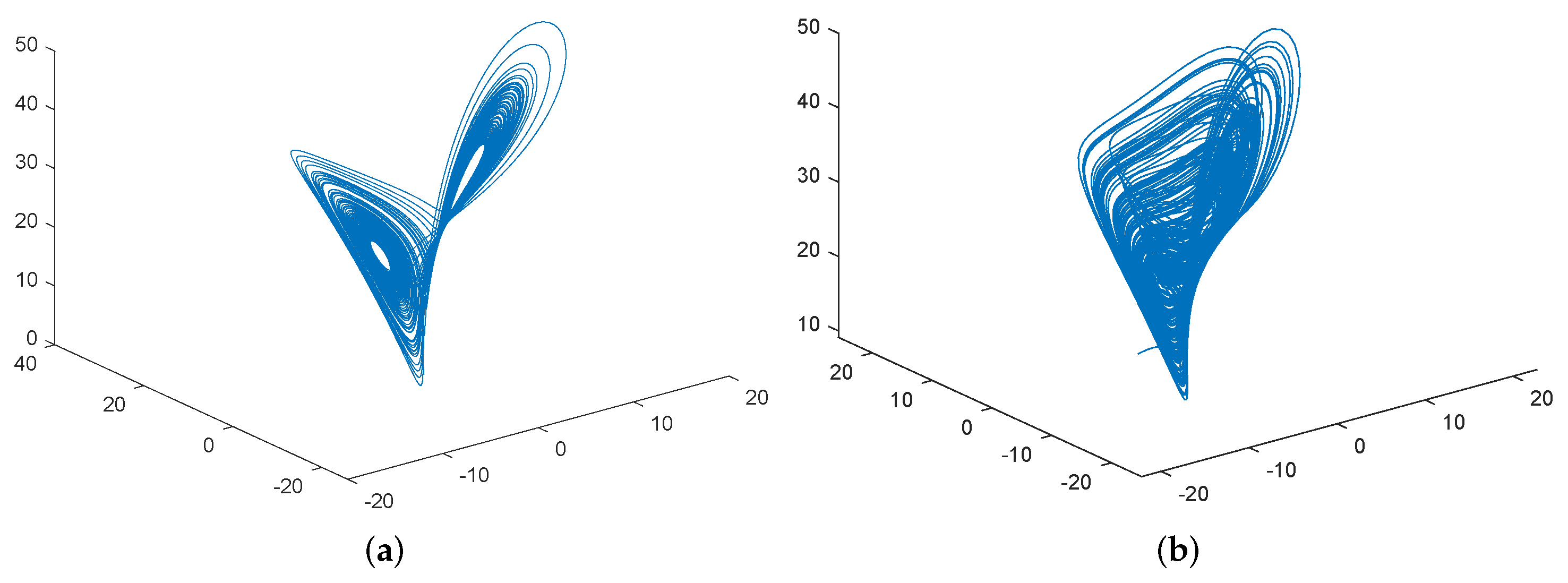
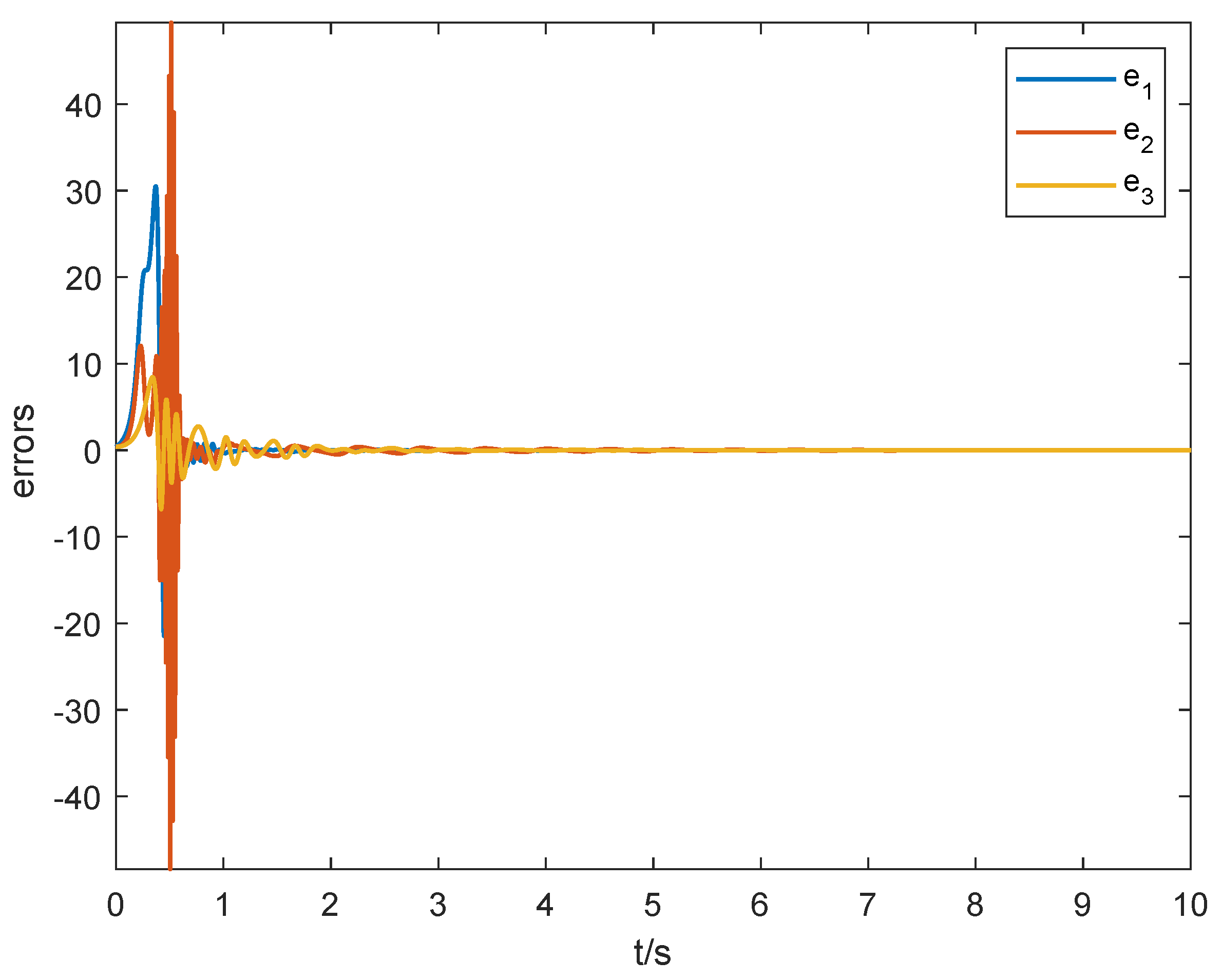
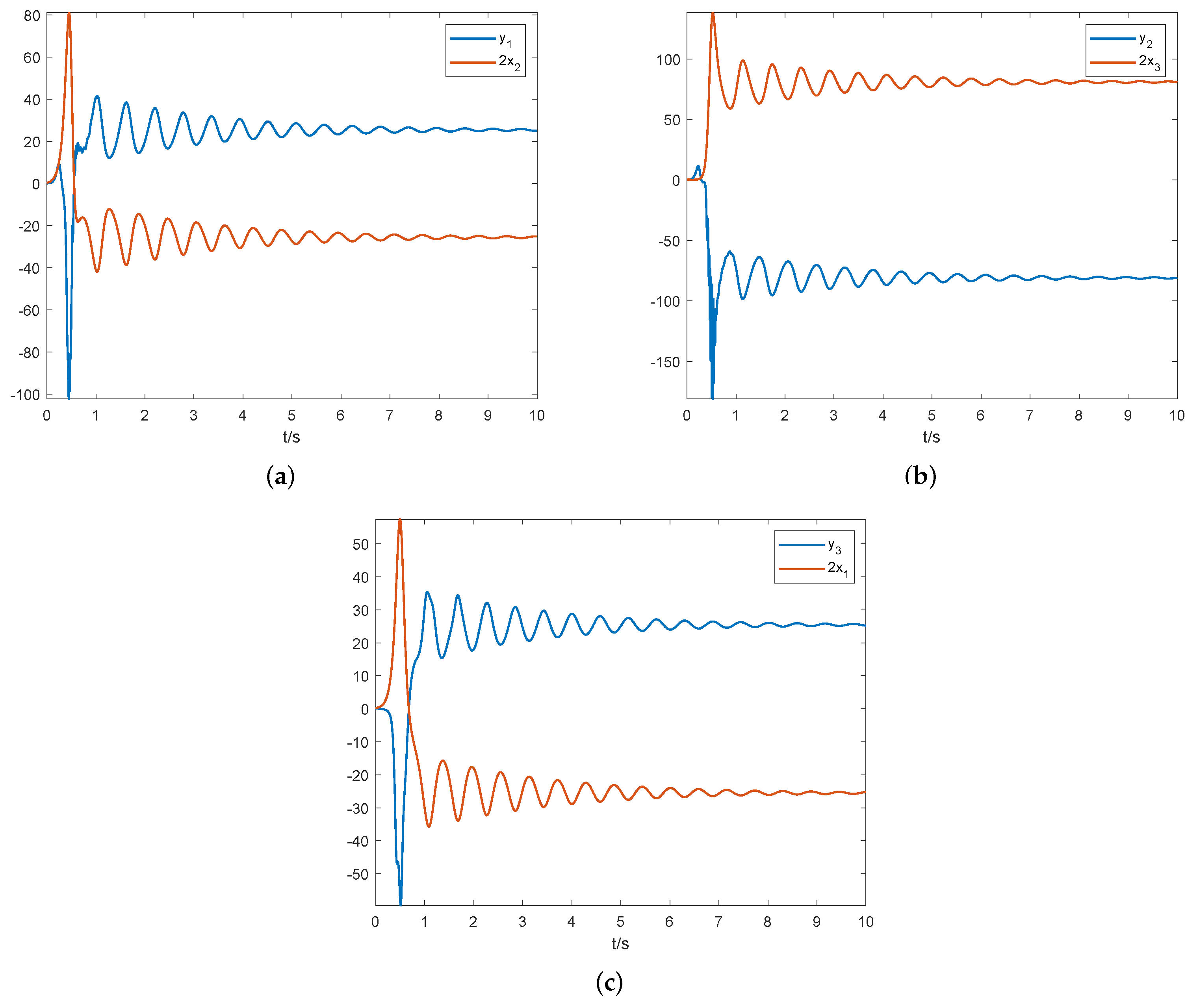
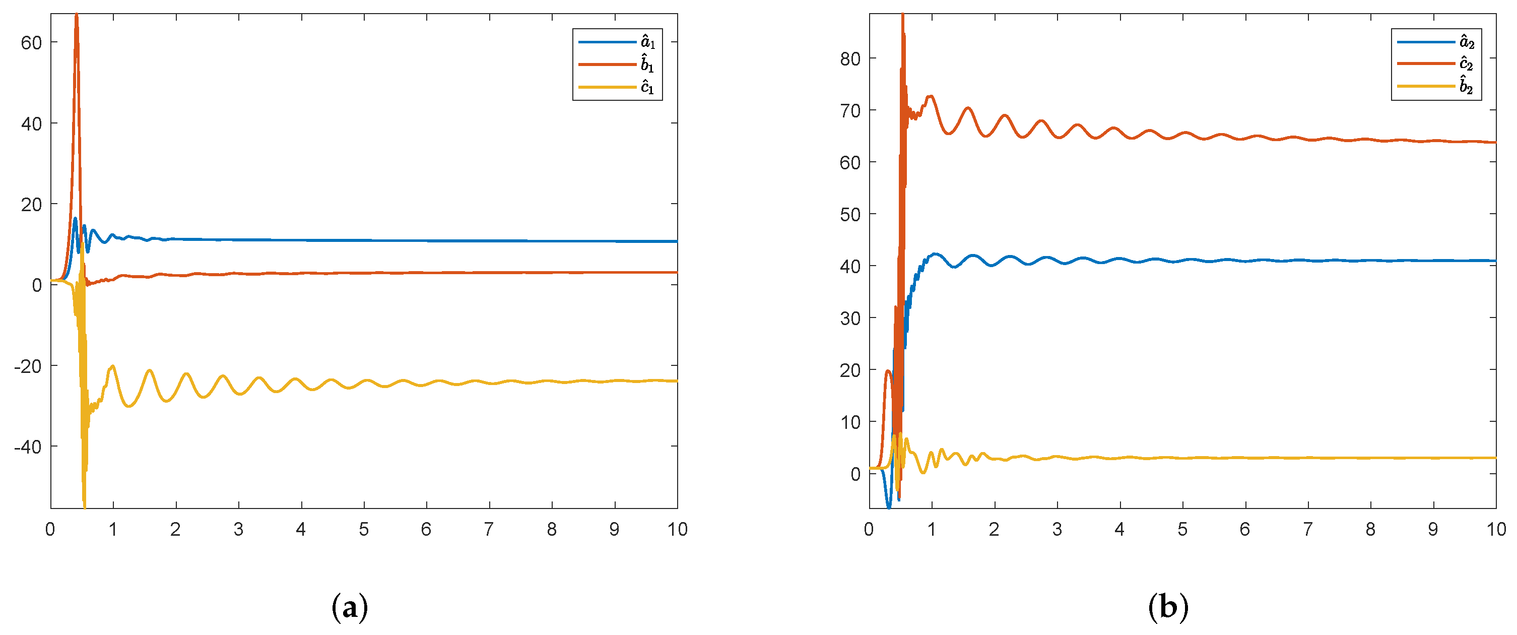
5.1. MSGPAS of Fractional Chaotic System

The fractional Lorenz chaotic system is selected as the drive system:

$$\left\{\begin{array}{c}{D}^{\omega }{x}_1\left(t\right)=a_1(x_2-x_1),\hfill \\ D^{\omega }{x}_2\left(t\right)=b_1{x}_1-x_1{x}_3-x_2,\hfill \\ D^{\omega }{x}_3\left(t\right)=-c_1{x}_3+x_1{x}_2,\hfill \end{array}\right.$$

(34)

where $x_i,i=1,2,3$ are the state variables, $a_1,b_1,c_1$ are the unknown parameters, and the drive system can be reformed as the following vector:

$$\begin{array}{c}\hfill D^{\mu }\mathit{x}\left(t\right)=\mathit{F}\left(\mathit{x}\left(t\right)\right)\mathit{\beta }+\mathit{f}(\mathit{x},t),\end{array}$$

(35)

where

$$\mathit{F}\left(\mathit{x}\left(t\right)\right)=\left[\begin{array}{ccc}{x}_2-x_1& 0& 0\\ 0& x_1& 0\\ 0& 0& -x_3\end{array}\right],\mathit{\beta }=\left[\begin{array}{c}{a}_1\\ b_1\\ c_1\end{array}\right],\mathit{f}(\mathit{x},t)=\left[\begin{array}{c}0\\ -x_1{x}_3-x_2\\ x_1{x}_2\end{array}\right].$$

(36)

The fractional Chen chaotic system with a controller is selected as the response system:

$$\left\{\begin{array}{c}{D}^{\omega }{y}_1\left(t\right)=a_2(y_2-y_1)+u_1,\hfill \\ D^{\omega }{y}_2\left(t\right)=-a_2{y}_1+c_2{y}_1+c_1{y}_2-y_1{y}_3+u_2,\hfill \\ D^{\omega }{y}_3\left(t\right)=-b_2{y}_3+y_1{y}_2+u_3,\hfill \end{array}\right.$$

(37)

where $y_i,i=1,2,3$ are the state variables, $a_2,c_2,b_2$ are the unknown parameters, and the response system can be reformed as the following vector:

$$\begin{array}{c}\hfill D^{\mu }\mathit{y}\left(t\right)=\mathit{G}\left(\mathit{y}\left(t\right)\right)\mathit{\eta }+\mathit{g}(\mathit{y},t)+\mathit{u}\left(t\right),\end{array}$$

(38)

where

$$\mathit{G}\left(\mathit{y}\left(t\right)\right)=\left[\begin{array}{ccc}{y}_2-y_1& 0& 0\\ -y_1& y_1+y_2& 0\\ 0& 0& -y_3\end{array}\right],\mathit{\eta }=\left[\begin{array}{c}{a}_2\\ c_2\\ b_2\end{array}\right],\mathit{g}(\mathit{y},t)=\left[\begin{array}{c}0\\ -y_1{y}_3\\ y_1{y}_2\end{array}\right].$$

(39)

We chose the parameters as $a_1=10,b_1=28,c_1=8/3,a_2=35,c_2=28,b_2=3$ [39], and the initial conditions were given as $x\left(0\right)=(0.1,0.1,0.1),y\left(0\right)=(-9,-5,14)$; taking the fractional-order $\omega =0.995$, we produced the chaotic trajectory shown in Figure 1.

According to the relationship Equation (25), we can obtain multiple multi-switch error state modes that can be combined as follows:

$$\begin{array}{cc}\hfill switch-1(i\ne j){:}_{12}e{,}_{13}e{,}_{21}e{,}_{23}e{,}_{31}e{,}_{32}e,& \\ & switch-2(i=j){:}_{11}e{,}_{22}e{,}_{33}e.\hfill \end{array}$$

(40)

We can choose any three errors from them as simulation metrics, such as

$$\left\{\begin{array}{c}{e}_1{=}_{12}e=y_1+a_{22}{x}_2,\hfill \\ e_2{=}_{23}e=y_2+a_{33}{x}_3,\hfill \\ e_3{=}_{31}e=y_3+a_{11}{x}_1,\hfill \end{array}\right.$$

(41)

where $a_{11},a_{22},a_{33}$ are the diagonal elements of projective matrix $\mathit{A}$. Thus, based on the definition of anti-synchronization error Equation (26), we can deduce the error system as follows:

$$\left\{\begin{array}{c}{D}^{\omega }{e}_1=D^{\omega }{(}_{12}e)=a_2(y_2-y_1)+a_{22}(b_1{x}_1-x_1{x}_3-x_2)+u_1,\hfill \\ D^{\omega }{e}_2=D^{\omega }{(}_{23}e)=-a_2{y}_1+c_2{y}_1+c_1{y}_2-y_1{y}_3+a_{33}(-c_1{x}_3+x_1{x}_2)+u_2,\hfill \\ D^{\omega }{e}_3=D^{\omega }{(}_{31}e)=-b_2{y}_3+y_1{y}_2+a_{11}\left(a_1(x_2-x_1)\right)+u_3.\hfill \end{array}\right.$$

(42)

It follows from Equations (28) and (31) that the controller is designed as

$$\left\{\begin{array}{c}{u}_1=a_{22}(x_1{x}_3+x_2)-{\widehat{a}}_2(y_2-y_1)-a_{22}{\widehat{b}}_1{x}_1-k{e}_1,\hfill \\ u_2=-a_{33}{x}_1{x}_2+y_1{y}_3+{\widehat{a}}_2{y}_1-{\widehat{c}}_2{y}_1-{\widehat{c}}_2{y}_2+a_{33}{\widehat{c}}_1{x}_3-k{e}_2,\hfill \\ u_3=-y_1{y}_2+{\widehat{b}}_2{y}_3-a_{11}{\widehat{a}}_1(x_2-x_1)-k{e}_3,\hfill \end{array}\right.$$

(43)

and the unknown parameter renewal laws are designed as

$$\left\{\begin{array}{c}{D}^{\omega }{\widehat{a}}_1=a_{11}(x_2-x_1)e_3,\hfill \\ D^{\omega }{\widehat{b}}_1=a_{22}{x}_1{e}_1,\hfill \\ D^{\omega }{\widehat{c}}_1=-a_{33}{x}_3{e}_2,\hfill \\ D^{\omega }{\widehat{a}}_2=(y_2-y_1)e_1-y_1{e}_2,\hfill \\ D^{\omega }{\widehat{c}}_2=(y_1+y_2)e_2,\hfill \\ D^{\omega }{\widehat{b}}_2=-y_3{e}_3,\hfill \end{array}\right.$$

(44)

and by substituting Equation (43) into Equation (42), the error system can be rewritten as

$$\left\{\begin{array}{c}{D}^{\omega }{e}_1=D^{\omega }{(}_{12}e)=-{\tilde{a}}_2(y_2-y_1)-a_{22}{\tilde{b}}_1{x}_1-k{e}_1,\hfill \\ D^{\omega }{e}_2=D^{\omega }{(}_{23}e)={\tilde{a}}_2{y}_1-{\tilde{c}}_2{y}_1-{\tilde{c}}_2{y}_2+a_{33}{\tilde{c}}_1{x}_3-k{e}_2,\hfill \\ D^{\omega }{e}_3=D^{\omega }{(}_{31}e)={\tilde{b}}_2{y}_3-a_{11}{\tilde{a}}_1(x_2-x_1)-k{e}_3.\hfill \end{array}\right.$$

(45)

Theorem 4.

The error system Equation (42) is asymptotically stable, i.e., system Equation (34) and system Equation (37) can realize MSGPAS via the generalized projective anti-synchronization adaptive controller (GPASAC) (43) and the generalized projective anti-synchronization adaptive renewal law (GPASARA) (44).

Proof. 

We take the Lyapunov function as

$$\begin{array}{c}\hfill V\left(t\right)={\displaystyle \frac{1}{2}}\sum _{i=1}^3{e}_i^2+{\displaystyle \frac{1}{2}}\sum _{i=1}^2({\tilde{a}}_i^2+{\tilde{b}}_i^2+{\tilde{c}}_i^2),\end{array}$$

(46)

and by taking the $\omega$-order derivative and making use of Equations (44) and (45), this yields

$$\begin{array}{cc}\hfill D^{\mu }V\left(t\right)& \le \sum _{i=1}^3{e}_i{D}^{\omega }{e}_i+\sum _{i=1}^2({\tilde{a}}_i{D}^{\omega }{\tilde{a}}_i+{\tilde{b}}_i{D}^{\omega }{\tilde{b}}_i+{\tilde{c}}_i{D}^{\omega }{\tilde{c}}_i)\hfill \\ \hfill & =-{\tilde{a}}_2(y_2-y_1)e_1-a_{22}{\tilde{b}}_1{x}_1{e}_1-k{e}_1^2\hfill \\ \hfill & +{\tilde{a}}_2{y}_1{e}_2-{\tilde{c}}_2{y}_1{e}_2-{\tilde{c}}_2{y}_2{e}_2+a_{33}{\tilde{c}}_1{x}_3{e}_2-k{e}_2^2\hfill \\ \hfill & +{\tilde{b}}_2{y}_3{e}_3-a_{11}{\tilde{a}}_1(x_2-x_1)e_3-k{e}_3^2\hfill \\ \hfill & +{\tilde{a}}_1\left[a_{11}(x_2-x_1)e_3\right]+{\tilde{b}}_1\left(a_{22}{x}_1{e}_1\right)+{\tilde{c}}_1(-a_{33}{x}_3{e}_2)\hfill \\ \hfill & +{\tilde{a}}_2[(y_2-y_1)e_1-y_1{e}_2]+{\tilde{c}}_2\left[(y_1+y_2)e_2\right]+{\tilde{b}}_2(-y_3{e}_3)\hfill \\ \hfill & =-k{e}_1^2-k{e}_2^2-k{e}_3^2\hfill \\ \hfill & \le 0,\hfill \end{array}$$

(47)

and consequently, based on Theorem 3, we can say the drive system Equation (34) and response system Equation (37) can realize MSGPAS via the generalized projective anti-synchronization adaptive controller (GPASAC) (43) and the generalized projective anti-synchronization adaptive renewal law (GPASARA) (44). □

In the simulatation progress, the projective matrix $\mathit{A}$ was set as $diag(2,2,2)$, the constant $k=1$, and the initial conditions for drive system (34) and response system (37) were assumed as $x\left(0\right)=(0.1,0.1,0.1)$ and $y\left(0\right)=(0.1,0.1,0.1)$. The initial conditions for the unknown parameters were assumed as $(a_1\left(0\right),b_1\left(0\right),c_1\left(0\right))=(1,1,1)$ and $(a_2\left(0\right),c_2\left(0\right),b_2\left(0\right))=(1,1,1)$ for the multi-switch error $\mathit{e}={(}_{12}e{,}_{23}e{,}_{31}e)$; the time response of the error state variables is shown in Figure 2. From the figure, it can be seen that the error states could converge to the origin in a relatively short time. The synchronization trajectory of drive system Equation (34) and response system Equation (37) are shown in Figure 3. The changing trajectory of the unknown parameters are shown in Figure 4, and all the simulation results reveal that the drive system Equation (34) and response system Equation (37) can realize MSGPAS via the generalized projective anti-synchronization adaptive controller (GPASAC) (43) and the generalized projective anti-synchronization adaptive renewal law (GPASARA) (44); this proves the correctness and rationality of our theory.

5.2. MSGPAS of Fractional Hyperchaotic System

The fractional Lorenz hyperchaotic system was selected as the drive system:

$$\left\{\begin{array}{c}{D}^{\omega }{x}_1\left(t\right)=a_1(x_2-x_1)+x_4,\hfill \\ D^{\omega }{x}_2\left(t\right)=b_1{x}_1-x_1{x}_3,\hfill \\ D^{\omega }{x}_3\left(t\right)=-c_1{x}_3+x_1{x}_2,\hfill \\ D^{\omega }{x}_4\left(t\right)=d_1{x}_4-x_2{x}_3,\hfill \end{array}\right.$$

(48)

where $x_i,i=1,2,3,4$ are the state variables, $a_1,b_1,c_1,d_1$ are the unknown parameters, and the drive system can be reformed as the following vector:

$$\begin{array}{c}\hfill D^{\mu }\mathit{x}\left(t\right)=\mathit{F}\left(\mathit{x}\left(t\right)\right)\mathit{\beta }+\mathit{f}(\mathit{x},t),\end{array}$$

(49)

where

$$\mathit{F}\left(\mathit{x}\left(t\right)\right)=\left[\begin{array}{cccc}{x}_2-x_1& 0& 0& 0\\ 0& x_1& 0& 0\\ 0& 0& -x_3& 0\\ 0& 0& 0& x_4\end{array}\right],\mathit{\beta }=\left[\begin{array}{c}{a}_1\\ b_1\\ c_1\\ d_1\end{array}\right],\mathit{f}(\mathit{x},t)=\left[\begin{array}{c}{x}_4\\ -x_1{x}_3\\ x_1{x}_2\\ -x_2{x}_3\end{array}\right].$$

(50)

The fractional Chen hyperchaotic system with a controller was selected as the response system:

$$\left\{\begin{array}{c}{D}^{\omega }{y}_1\left(t\right)=a_2(y_2-y_1)+y_4+u_1,\hfill \\ D^{\omega }{y}_2\left(t\right)=c_2{y}_2+d_2{y}_1-y_1{y}_3+u_2,\hfill \\ D^{\omega }{y}_3\left(t\right)=-b_2{y}_3+y_1{y}_2+u_3,\hfill \\ D^{\omega }{y}_4\left(t\right)=r{y}_4+y_2{y}_3+u_4,\hfill \end{array}\right.$$

(51)

where $y_i,i=1,2,3,4$ are the state variables, $a_2,b_2,c_2,d_2,r$ are the unknown parameters, and the response system can be reformed as the following vector:

$$\begin{array}{c}\hfill D^{\mu }\mathit{y}\left(t\right)=\mathit{G}\left(\mathit{y}\left(t\right)\right)\mathit{\eta }+\mathit{g}(\mathit{y},t)+\mathit{u}\left(t\right),\end{array}$$

(52)

where

$$\mathit{G}\left(\mathit{y}\left(t\right)\right)=\left[\begin{array}{ccccc}{y}_2-y_1& 0& 0& 0& 0\\ 0& 0& y_2& y_1& 0\\ 0& -y_3& 0& 0& 0\\ 0& 0& 0& 0& y_4\end{array}\right],\mathit{\eta }=\left[\begin{array}{c}{a}_2\\ b_2\\ c_2\\ d_2\\ r\end{array}\right],\mathit{g}(\mathit{y},t)=\left[\begin{array}{c}{y}_4\\ -y_1{y}_3\\ y_1{y}_2\\ y_2{y}_3\end{array}\right].$$

(53)

We chose the parameters as $a_1=10,b_1=28,c_1=8/3,d_1=-1,a_2=35,b_2=32,$$c_2=12,d_2=7,r=0.5$ [39], and the initial conditions were given as $x\left(0\right)=(2,2,1,1),y\left(0\right)=(1,1,2,2)$; taking the fractional-order $\omega =0.99$, we produced the hyperchaotic trajectory shown in Figure 5.

According to the relationship Equation (25), we can obtain multiple multi-switch error state modes that can be combined as follows:

$$\begin{array}{cc}\hfill switch-1(i\ne j):& {}_{12}e,{}_{13}e,{}_{14}e,\hfill \\ & {}_{21}e,{}_{23}e,{}_{24}e,\hfill \\ & {}_{31}e,{}_{32}e,{}_{34}e,\hfill \\ & {}_{41}e,{}_{42}e,{}_{43}e,\hfill \\ \hfill switch-2(i=j):& {}_{11}e,{}_{22}e,{}_{33}e,{}_{44}e.\hfill \end{array}$$

(54)

We can choose any four errors from them as simulation metrics, such as

$$\left\{\begin{array}{c}{e}_1{=}_{12}e=y_1+a_{22}{x}_2,\hfill \\ e_2{=}_{23}e=y_2+a_{33}{x}_3,\hfill \\ e_3{=}_{34}e=y_3+a_{44}{x}_4,\hfill \\ e_4{=}_{41}e=y_4+a_{11}{x}_1,\hfill \end{array}\right.$$

(55)

where $a_{11},a_{22},a_{33},a_{44}$ are the diagonal elements of projective matrix $\mathit{A}$. Thus, based on the definition of anti-synchronization error Equation (26), we can deduce the error system as follows:

$$\left\{\begin{array}{c}{D}^{\omega }{e}_1=D^{\omega }{(}_{12}e)=a_2(y_2-y_1)+y_4+a_{22}(b_1{x}_1-x_1{x}_3)+u_1,\hfill \\ D^{\omega }{e}_2=D^{\omega }{(}_{23}e)=c_2{y}_2+d_2{y}_1-y_1{y}_3+a_{33}(-c_1{x}_3+x_1{x}_2)+u_2,\hfill \\ D^{\omega }{e}_3=D^{\omega }{(}_{34}e)=-b_2{y}_3+y_1{y}_2+a_{44}(d_1{x}_4-x_2{x}_3)+u_3,\hfill \\ D^{\omega }{e}_4=D^{\omega }{(}_{41}e)=r{y}_4+y_2{y}_3+a_{11}[a_1(x_2-x_1)+x_4]+u_4.\hfill \end{array}\right.$$

(56)

It follows from Equations (28) and (31) that the controller is designed as

$$\left\{\begin{array}{c}{u}_1=-y_4+a_{22}{x}_1{x}_3-{\widehat{a}}_2(y_2-y_1)-a_{22}{\widehat{b}}_1{x}_1-k{e}_1,\hfill \\ u_2=y_1{y}_3-a_{33}{x}_1{x}_2-{\widehat{c}}_2{y}_2-{\widehat{d}}_2{y}_1+a_{33}{\widehat{c}}_1{x}_3-k{e}_2,\hfill \\ u_3=-y_1{y}_2+a_{44}{x}_2{x}_3+{\widehat{b}}_2{y}_3-a_{44}{\widehat{d}}_1{x}_4-k{e}_3,\hfill \\ u_4=-y_2{y}_3-a_{11}{x}_4-r{y}_4-a_{11}{\widehat{a}}_1(x_1-x_1)-k{e}_4,\hfill \end{array}\right.$$

(57)

and the unknown parameter renewal laws is designed as

$$\left\{\begin{array}{c}{D}^{\omega }{\widehat{a}}_1=a_{11}(x_2-x_1)e_4,D^{\omega }{\widehat{b}}_1=a_{22}{x}_1{e}_1,\hfill \\ D^{\omega }{\widehat{c}}_1=-a_{33}{x}_3{e}_2,D^{\omega }{\widehat{d}}_1=a_{44}{x}_4{e}_3,\hfill \\ D^{\omega }{\widehat{a}}_2=(y_2-y_1)e_1,D^{\omega }{\widehat{b}}_2=-y_3{e}_3,\hfill \\ D^{\omega }{\widehat{c}}_2=y_2{e}_2,D^{\omega }{\widehat{d}}_2=y_1{e}_2,\hfill \\ D^{\omega }\widehat{r}=y_4{e}_4,\hfill \end{array}\right.$$

(58)

and by substituting Equation (57) into Equation (56), the error system can be rewritten as

$$\left\{\begin{array}{c}{D}^{\omega }{e}_1=D^{\omega }{(}_{12}e)=-{\tilde{a}}_2(y_2-y_1)-a_{22}{\tilde{b}}_1{x}_1-k{e}_1,\hfill \\ D^{\omega }{e}_2=D^{\omega }{(}_{23}e)=-{\tilde{c}}_2{y}_2-{\tilde{d}}_2{y}_1+a_{33}{\tilde{c}}_1{x}_3-k{e}_2,\hfill \\ D^{\omega }{e}_3=D^{\omega }{(}_{34}e)={\tilde{b}}_2{y}_3-a_{44}{\tilde{d}}_1{x}_4-k{e}_3,\hfill \\ D^{\omega }{e}_4=D^{\omega }{(}_{41}e)=-\tilde{r}{y}_4-a_{11}{\tilde{a}}_1(x_2-x_1)-k{e}_4.\hfill \end{array}\right.$$

(59)

Theorem 5.

The error system Equation (56) is asymptotically stable, i.e., system Equation (48) and system Equation (51) can realize MSGPAS via the generalized projective anti-synchronization adaptive controller (GPASAC) (57) and the generalized projective anti-synchronization adaptive renewal law (GPASARA) (58).

Proof. 

We take the Lyapunov function as

$$\begin{array}{c}\hfill V\left(t\right)={\displaystyle \frac{1}{2}}\sum _{i=1}^4{e}_i^2+{\displaystyle \frac{1}{2}}\sum _{i=1}^2({\tilde{a}}_i^2+{\tilde{b}}_i^2+{\tilde{c}}_i^2+{\tilde{d}}_i^2)+{\displaystyle \frac{1}{2}}{\tilde{r}}^2,\end{array}$$

(60)

and by taking the $\omega$-order derivative and making use of Equations (58) and (59), this yields

$$\begin{array}{cc}\hfill D^{\mu }V\left(t\right)& \le \sum _{i=1}^4{e}_i{D}^{\omega }{e}_i+\sum _{i=1}^2({\tilde{a}}_i{D}^{\omega }{\tilde{a}}_i+{\tilde{b}}_i{D}^{\omega }{\tilde{b}}_i+{\tilde{c}}_i{D}^{\omega }{\tilde{c}}_i+{\tilde{d}}_i{D}^{\omega }{\tilde{d}}_i)+\tilde{r}{D}^{\omega }\tilde{r}\hfill \\ & =-{\tilde{a}}_2(y_2-y_1)e_1-a_{22}{\tilde{b}}_1{x}_1{e}_1-k{e}_1^2\hfill \\ & -{\tilde{c}}_2{y}_2{e}_2-{\tilde{d}}_2{y}_1{e}_2+a_{33}{\tilde{c}}_1{x}_3{e}_2-k{e}_2^2\hfill \\ & +{\tilde{b}}_2{y}_3{e}_3-a_{44}{\tilde{d}}_1{x}_4{e}_3-k{e}_3^2\hfill \\ & -\tilde{r}{y}_4{e}_4-a_{11}{\tilde{a}}_1(x_2-x_1)e_4-k{e}_4^2\hfill \\ & +{\tilde{a}}_1(x_2-x_1)a_{11}{e}_4+{\tilde{b}}_1{x}_1{a}_{22}{e}_1+{\tilde{c}}_1(-x_3{a}_{33}{e}_2)+{\tilde{d}}_1{x}_4{a}_{44}{e}_3\hfill \\ & +{\tilde{a}}_2(y_2-y_1)e_1+{\tilde{b}}_2(-y_3{e}_3)+{\tilde{c}}_2\left(y_2{e}_2\right)+{\tilde{d}}_2{y}_1{e}_2+\tilde{r}{y}_4{e}_4\hfill \\ & =-k{e}_1^2-k{e}_2^2-k{e}_3^2-k{e}_4^2\hfill \\ & \le 0,\hfill \end{array}$$

(61)

and consequently, based on Theorem 3, we can say that the drive system Equation (48) and response system Equation (51) can realize MSGPAS via the generalized projective anti-synchronization adaptive controller (GPASAC) (57) and the generalized projective anti-synchronization adaptive renewal law (GPASARA) (58). □

In the simulation progress, the projective matrix $\mathit{A}$ was set as $diag(2,2,2,2)$, the constant $k=1$, and the initial conditions for drive system (48) and response system (51) were assumed as $x\left(0\right)=(0.1,0.1,0.1,0.1)$ and $y\left(0\right)=(0.1,0.1,0.1,0.1)$. The initial conditions for the unknown parameters were assumed as $(a_1\left(0\right),b_1\left(0\right),c_1\left(0\right),d_1\left(0\right))=(1,1,1,1)$, $(a_2\left(0\right),b_2\left(0\right),c_2\left(0\right),d_2\left(0\right),r\left(0\right))=(1,1,1,1,1)$; for the multi-switch error $\mathit{e}={(}_{12}e{,}_{23}e{,}_{34}e{,}_{41}e)$, the time response of the error state variables is shown in Figure 6. From the figure, it can be seen that the error state could converge to the origin in a relatively short time. The synchronization trajectory of drive system Equation (48) and response system Equation (51) are shown in Figure 7, and the changing trajectory of the unknown parameters are shown in Figure 8; all the simulation results reveal that the drive system Equation (48) and response system Equation (51) can realize MSGPAS via the generalized projective anti-synchronization adaptive controller (GPASAC) defined in Equation (57) and the generalized projective anti-synchronization adaptive renewal law (GPASARA) defined in Equation (58); this proves the correctness and rationality of our theory.

6. Conclusions

In this manuscript, the multi-switching generalized projection anti-synchronization problem of fractional-order chaotic systems has been investigated. The model is formulated in the Caputo–Fabrizio sense, with system parameters being unknown. Initially, a new fractional-order differential inequality is proven, which facilitates the identification of a suitable Lyapunov function. Subsequently, appropriate and precise controllers, along with adaptive laws for unknown parameters, are designed to achieve synchronization of the system under consideration. In the end, the significance of the suggested theoretical approach has been demonstrated through two numerical examples. Future work will focus on achieving synchronization of the error systems within finite or fixed time, aiming to address certain limitations of the current research.

References

1. Butzer, P.L.; Westphal, U. An introduction to fractional calculus. In Applications of Fractional Calculus in Physics; World Scientific Publishing: Singapore, 2000; pp. 1–85. [Google Scholar]
2. Chen, L.P.; Liu, C.; Lopes, A.M.; Lin, Y.; Liu, Y.X.; Chen, Y.Q. LMI synchronization conditions for variable fractional-order one-sided Lipschitz chaotic systems with gain fluctuations. Chaos Solitons Fractals 2024, 189, 115695. [Google Scholar] [CrossRef]
3. Eshaghi, S.; Kadkhoda, N.; Inc, M. Chaos control and synchronization of a new fractional laser chaotic system. Qual. Theory Dyn. Syst. 2024, 23, 241. [Google Scholar] [CrossRef]
4. Han, T.; Zhang, K.; Jiang, Y.; Rezazadeh, H. Chaotic Pattern and Solitary Solutions for the (21)-Dimensional Beta-Fractional Double-Chain DNA System. Fractal Fract. 2024, 8, 415. [Google Scholar] [CrossRef]
5. Mo, W.; Bao, H. Mean-square bounded synchronization of fractional-order chaotic Lure systems under deception attack. Phys. A Stat. Mech. Appl. 2024, 641, 129726. [Google Scholar] [CrossRef]
6. Puente-Cordova, J.G.; Rentera-Baltirrez, F.Y.; Lopez-Walle, B.; LOpez-Walle, B.; Aguilar-Garib, J.A. Dielectric and Viscoelastic Behavior of Polyvinyl Butyral Films. Polymers 2023, 15, 4725. [Google Scholar] [CrossRef]
7. Pecora, L.M.; Carroll, T.L. Synchronization in chaotic systems. Phys. Rev. Lett. 1990, 64, 821. [Google Scholar] [CrossRef] [PubMed]
8. Ojo, K.S.; Ogunjo, S.T.; Fuwape, I.A. Modified hybrid combination synchronization of chaotic fractional order systems. Soft Comput. 2022, 26, 11865–11872. [Google Scholar] [CrossRef]
9. Yadav, V.K.; Kumar, R.; Leung, A.Y.T.; Das, S. Dual phase and dual anti-phase synchronization of fractional order chaotic systems in real and complex variables with uncertainties. Chin. J. Phys. 2019, 57, 282–308. [Google Scholar] [CrossRef]
10. Hamoudi, A.; Djeghali, N.; Bettayeb, M. High-order sliding mode-based synchronisation of fractional-order chaotic systems subject to output delay and unknown disturbance. Int. J. Syst. Sci. 2022, 53, 2876–2900. [Google Scholar] [CrossRef]
11. Wang, F.; Zheng, Z. Quasi-projective synchronization of fractional order chaotic systems under input saturation. Phys. A Stat. Mech. Appl. 2019, 534, 122132. [Google Scholar] [CrossRef]
12. Li, B.; Zhou, X.; Wang, Y. Combination Synchronization of Three Different Fractional-Order Delayed Chaotic Systems. Complexity 2019, 2019, 5184032. [Google Scholar] [CrossRef]
13. Talebi, S.P.; Godsill, S.J.; Mandic, D.P. Filtering structures for α-stable systems. IEEE Control. Syst. Lett. 2022, 7, 553–558. [Google Scholar] [CrossRef]
14. Bendoukha, S.; Abdelmalek, S. The fractional chua chaotic system: Dynamics, synchronization, and application to secure communications. Int. J. Nonlinear Sci. Numer. Simul. 2019, 20, 77–88. [Google Scholar] [CrossRef]
15. Mansouri, D.; Bendoukha, S.; Abdelmalek, S.; Youkana, A. On the complete synchronization of a time-fractional reactionCdiffusion system with the NewtonCLeipnik nonlinearity. Appl. Anal. 2021, 100, 675–694. [Google Scholar] [CrossRef]
16. Gupta, S.; Varshney, P.; Srivastava, S. Whale optimization based synchronization and control of two identical fractional order financial chaotic systems. J. Intell. Fuzzy Syst. 2022, 42, 929–942. [Google Scholar] [CrossRef]
17. Almuzaini, M.; Alzahrani, A. Control and synchronization of a novel realizable nonlinear chaotic system. Fractal Fract. 2023, 7, 253. [Google Scholar] [CrossRef]
18. Echenausa-Monroy, J.L.; Rodrguez-Martne, C.A.; Alvarez, J.; Ramirez, J.P. Synchronization in Dynamically Coupled Fractional-Order Chaotic Systems: Studying the Effects of Fractional Derivatives. Complexity 2021, 2021, 7242253. [Google Scholar] [CrossRef]
19. Shao, K.; Guo, H.; Han, F. Finite-time projective synchronization of fractional-order chaotic systems via soft variable structure control. J. Mech. Sci. Technol. 2020, 34, 369–376. [Google Scholar] [CrossRef]
20. Meng, X.; Wu, Z.; Gao, C.; Jiang, B.; Karimi, H.R. Finite-time projective synchronization control of variable-order fractional chaotic systems via sliding mode approach. IEEE Trans. Circuits Syst. II Express Briefs 2021, 68, 2503–2507. [Google Scholar] [CrossRef]
21. Ouannas, A.; Khennaoui, A.A.; Zehrour, O.; Bendoukha, S.; Grassi, G.; Pham, V.T. Synchronisation of integer-order and fractional-order discrete-time chaotic systems. Pramana 2019, 92, 52. [Google Scholar] [CrossRef]
22. Zhang, R.; Liu, Y.; Yang, S. Adaptive synchronization of fractional-order complex chaotic system with unknown complex parameters. Entropy 2019, 21, 207. [Google Scholar] [CrossRef] [PubMed]
23. Zhang, R.; Feng, S.; Yang, S. Complex Modified Projective Synchronization of Fractional-order Complex-Variable Chaotic System with Unknown Complex Parameters. Entropy 2019, 21, 407. [Google Scholar] [CrossRef]
24. Almatroud, A.O. Synchronisation of two different uncertain fractional-order chaotic systems with unknown parameters using a modified adaptive sliding-mode controller. Adv. Differ. Equ. 2020, 2020, 78. [Google Scholar] [CrossRef]
25. Liu, D.; Li, T.; Wang, Y. Adaptive dual synchronization of fractional-order chaotic system with uncertain parameters. Mathematics 2022, 10, 470. [Google Scholar] [CrossRef]
26. Sabaghian, A.; Balochian, S.; Yaghoobi, M. Synchronisation of 6D hyper-chaotic system with unknown parameters in the presence of disturbance and parametric uncertainty with unknown bounds. Connect. Sci. 2020, 32, 362–383. [Google Scholar] [CrossRef]
27. Pan, W.; Li, T.; Sajid, M.; Pu, L. Parameter identification and the finite-time combinationCcombination synchronization of fractional-order chaotic systems with different structures under multiple stochastic disturbances. Mathematics 2022, 10, 712. [Google Scholar] [CrossRef]
28. Hailong, Z.; Ding, Z.; Wang, L. Predefined-time multi-switch combination-combination synchronization of fractional-order chaotic systems with time delays. Phys. Scr. 2024, 99, 105223. [Google Scholar] [CrossRef]
29. Li, B.; Wang, Y.; Zhou, X. Multi-switching combination synchronization of three fractional-order delayed Systems. Appl. Sci. 2019, 9, 4348. [Google Scholar] [CrossRef]
30. Shahzad, M. Exploring the Different Order of Switches During Multi-switching Synchronization. Iran. J. Sci. 2024, 48, 965–977. [Google Scholar] [CrossRef]
31. Sayed, W.S.; Radwan, A.G. Generalized switched synchronization and dependent image encryption using dynamically rotating fractional-order chaotic systems. AEU-Int. J. Electron. Commun. 2020, 123, 153268. [Google Scholar] [CrossRef]
32. Sabzalian, M.H.; Mohammadzadeh, A.; Zhang, W.; Jermsittiparsert, K. General type-2 fuzzy multi-switching synchronization of fractional-order chaotic systems. Eng. Appl. Artif. Intell. 2021, 100, 104163. [Google Scholar] [CrossRef]
33. Pan, W.; Li, T.; Wang, Y. The multi-switching sliding mode combination synchronization of fractional order non-identical chaotic system with stochastic disturbances and unknown parameters. Fractal Fract. 2022, 6, 102. [Google Scholar] [CrossRef]
34. Liu, D.; Li, T.; He, X. Fixed-Time Multi-Switch Combined-Combined Synchronization of Fractional-Order Chaotic Systems with Uncertainties and External Disturbances. Fractal Fract. 2023, 7, 281. [Google Scholar] [CrossRef]
35. Caputo, M.; Fabrizio, M. A new definition of fractional derivative without singular kernel. Prog. Fract. Differ. Appl. 2015, 1, 73–85. [Google Scholar]
36. Losada, J.; Nieto, J.J. Properties of a new fractional derivative without singular kernel. Prog. Fract. Differ. Appl. 2015, 1, 87–92. [Google Scholar]
37. Salahshour, S.; Ahmadian, A.; Salimi, M.; Pansera, B.A.; Ferrara, M. A new Lyapunov stability analysis of fractional-order systems with nonsingular kernel derivative. Alex. Eng. J. 2020, 59, 2985–2990. [Google Scholar] [CrossRef]
38. Toh, Y.T.; Phang, C.; Loh, J.R. New predictor-corrector scheme for solving nonlinear differential equations with Caputo-Fabrizio operator. Math. Methods Appl. Sci. 2019, 42, 175–185. [Google Scholar] [CrossRef]
39. Petrás, I. Fractional-Order Nonlinear Systems: Modeling, Analysis and Simulation; Springer Science & Business Media: Berlin/Heidelberg, Germany, 2011. [Google Scholar]
Figure 1. The chaotic trajectories of fractional Lorenz and Chen chaotic systems in sub-figure (a,b), respectively.
Symmetry 17 00957 g001
Figure 2. The time response of error state variables e 1 , e 2 , e 3 .
Symmetry 17 00957 g002
Figure 3. The anti-synchronization trajectory of y 1 and 2 x 2 , y 2 and 2 x 3 , and y 3 and 2 x 1 from (ac), respectively.
Symmetry 17 00957 g003
Figure 4. The estimated value of the unknown parameters (a) a 1 , b 1 , c 1 and (b) a 2 , c 2 , b 2 .
Symmetry 17 00957 g004
Figure 5. The chaotic trajectories of fractional Lorenz and Chen hyperchaotic systems in sub-figure (a,b), respectively.
Symmetry 17 00957 g005
Figure 6. The time response of error state variables e 1 , e 2 , e 3 , e 4 .
Symmetry 17 00957 g006
Figure 7. The anti-synchronization trajectory of y 1 and 2 x 2 , y 2 and 2 x 3 , y 3 and 2 x 4 , and y 4 and 2 x 1 from (ad), respectively.
Symmetry 17 00957 g007
Figure 8. The estimated value of the unknown parameters (a) a 1 , b 1 , c 1 , d 1 and (b) a 2 , b 2 , c 2 , d 2 , r .
Symmetry 17 00957 g008
Disclaimer/Publisher’s Note: The statements, opinions and data contained in all publications are solely those of the individual author(s) and contributor(s) and not of MDPI and/or the editor(s). MDPI and/or the editor(s) disclaim responsibility for any injury to people or property resulting from any ideas, methods, instructions or products referred to in the content.