Symmetry-Aware CVAE-ACGAN-Based Feature Generation Model and Its Application in Fault Diagnosis

Abstract

Traditional fault feature generation models often face issues of uncontrollability, singularity, and slow convergence, limiting diagnostic accuracy. To address these challenges, this paper proposes a symmetry-aware approach that combines a conditional variational autoencoder (CVAE) and an auxiliary classifier generative adversarial network (ACGAN) for fault feature generation, leveraging symmetry characteristics inherent in fault data distributions and adversarial learning. Specifically, symmetrical Gaussian distributions in the CVAE enable robust extraction of latent fault features conditioned on fault classes, which are then input to the symmetrical adversarial framework of the ACGAN to guide the generator and discriminator toward a symmetrical Nash equilibrium. The original and generated features are jointly utilized in a convolutional neural network (CNN) for fault classification. Experimental results on the CWRU dataset show that the proposed CVAE-ACGAN achieves an average accuracy of 99.21%, precision of 97.81%, and recall of 98.24%, surpassing the baseline CNN. Similar improvements are achieved on the PADERBORN dataset. Furthermore, the model achieves significantly lower root mean square error (RMSE) and mean absolute error (MAE) than competing methods, confirming high consistency between the generated and real features and supporting its superior generalization and reliability. Visualization via confusion matrices and t-SNE further demonstrates clear boundaries between fault categories. These results affirm the value of incorporating symmetry principles into feature generation for mechanical fault diagnosis.

1. Introduction

Bearings are critical components in mechanical equipment, and their frequent failures often disrupt normal operations, leading to substantial economic losses [1,2,3]. Consequently, the timely and effective diagnosis of bearing faults holds paramount importance in engineering practice. In recent years, advancements in deep learning have catalyzed its application in fault diagnosis, yielding impressive results. For example, Mao [4] proposed a deep autoencoder method incorporating identification information, which enhances feature representation without requiring fine-tuning and improves model stability, particularly when training data is limited. Liu [5] introduced a composite fault diagnosis approach using zero-shot learning, where monotonic fault vibration data models are utilized to identify unknown hybrid faults, eliminating the need for expert intervention in handling semantic vectors of monotonic and composite faults. Zhang [6] developed a novel nonconvex generalized logarithmic (G-LOG) penalty for sparse representation, preserving the convexity of the cost function through parameter matrix adjustments. This method also introduces k-sparsity for adaptive regularization parameter selection, achieving superior reconstruction accuracy in both simulations and experiments. She [7] proposed a fault diagnosis method employing a deep convolutional variational autoencoder network (DCVAEN), which addresses various fault types and operating conditions while demonstrating robust generalization capabilities. Similarly, Dong [8] presented a diagnostic technique leveraging multi-layer noise reduction and an improved convolutional neural network (ICNN), enabling fault diagnosis with enhanced accuracy and generalization in noise-heavy environments. These studies primarily rely on extensive, high-quality fault datasets for model training. Ali [9] explored the mathematical analysis of intrinsic mode function (IMF) derived from empirical mode decomposition (EMD) energy entropy, demonstrating that the extracted features effectively train artificial neural networks (ANNs) to classify bearing defects with high accuracy. While traditional fault diagnosis methods for rolling bearings heavily depend on large-scale practical datasets, real-world industrial scenarios often involve data characterized by high noise, variability in working conditions, monotonicity, uncertainty, and high acquisition costs [10,11,12]. Such challenges hinder the availability of reliable and effective fault diagnosis datasets, thereby limiting the accuracy and generalization capabilities of conventional models [13,14]. From a statistical-signal-analysis standpoint, baseline bearing-vibration signals exhibit an almost Gaussian symmetry, whereas the onset of faults perturbs this balance and introduces controlled asymmetry in both amplitude and frequency components. Systematically recognizing and exploiting this symmetry–asymmetry transition provides a principled foundation for feature extraction and guides the architecture of the generative models proposed in this study.

To address these issues, researchers have explored data augmentation (DA) and generative approaches. Liu [15] proposed a generative adversarial network (GAN)-based DA strategy to expand imbalanced sample datasets. By utilizing multiple similarity indicators to evaluate the quality of generated data, the study developed a federated cabinet model for unbalanced fault diagnosis and extracted fault-sensitive features, demonstrating strong performance on highly imbalanced datasets. Liu [16] improved the GAN framework by incorporating an encoder for deep feature learning and applying depth regret analysis to prevent pattern collapse in the discriminator. Additionally, the generator employed a feature-matching module to enhance data quality. Liang [17] combined wavelet transform (WT), GAN, and convolutional neural networks (CNN) in the WT-GAN-CNN model, achieving higher diagnostic accuracy in environments with significant noise or variable conditions. Gao [18] introduced a fault multi-classification method based on the conditional variational autoencoder-CNN (CVAE-CNN), which improves the recognition rate of under-represented fault categories by extracting complex hidden features. Similarly, Dai [19] proposed combining GAN with an autoencoder (AE) to train and optimize feature generation models through encoding, decoding, and re-decoding processes. Guo [20] developed the multi-label one-dimensional GAN (ML1-D-GAN), which generates realistic fault data to train classifiers, enhancing diagnostic accuracy and improving model performance.

Despite the promise of these approaches, existing methods often neglect the class attributes of original data and face challenges with convergence during feature generation. While the conditional variational autoencoder (CVAE) assumes a Gaussian distribution for observed data [21,22,23], it lacks the precision required for accurate feature extraction [24,25]. Conversely, the flexibility of GAN training introduces difficulties in constraining generated features [26]. The auxiliary classifier GAN (ACGAN) improves GANs by introducing an auxiliary classifier to guide the generation of conditional features [27]. However, the ACGAN suffers from slow convergence, monotonicity, and instability during feature extraction [28,29,30,31], limiting the accuracy, precision, and generalization of fault diagnosis models.

Specifically, existing models present several critical limitations. The CVAE assumes a strict Gaussian distribution of observed data, which rarely aligns with real-world fault data, characterized by noise and non-stationarity, thus reducing accuracy and generalization. GAN-based models, though powerful, frequently encounter issues such as mode collapse, uncontrollable feature generation, and unstable training, undermining their reliability. Similarly, the ACGAN improves conditional generation but still suffers from slow convergence and instability. To address these constraints, the proposed symmetry-aware CVAE-ACGAN integrates symmetry properties explicitly into latent distributions and adversarial dynamics, enhancing stability and generalization in fault diagnosis.

Motivated by these observations, we design a symmetry-aware CVAE-ACGAN (abbreviated as CVAE-ACGAN) that explicitly exploits the near-Gaussian symmetry of baseline vibration signals and the symmetric adversarial dynamics of GAN training. The proposed CVAE-ACGAN feature generation model is then evaluated with a CNN-based fault diagnosis classifier. The main contributions of this work are as follows:

• A method is introduced to address the challenges of acquiring failure data in mechanical equipment, particularly data monotonicity and uncontrollability, which impede diagnostic accuracy. The proposed model incorporates the categorical attributes of fault data, enhancing controllability and reducing monotonicity, thereby enabling the generation of effective class-conditional features.
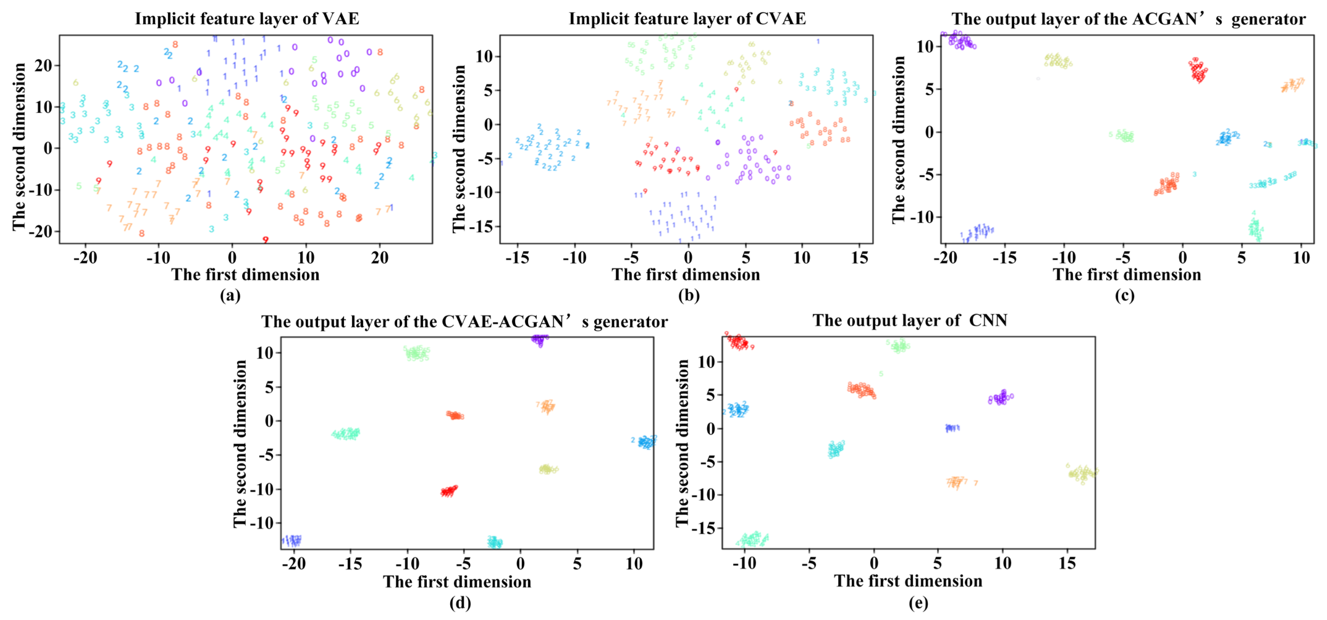
• A thorough comparison of feature generation models is conducted using four performance metrics: accuracy, precision, recall, and average results. The proposed features are evaluated through diagnostic outcomes, confusion matrices, and t-SNE visualizations. The experimental results demonstrate that the proposed model outperforms existing approaches in terms of accuracy, precision, stability, and convergence speed.
• In addition to conventional classification metrics, this work introduces root mean square error (RMSE) and mean absolute error (MAE) to quantitatively assess the similarity between generated features and real vibration data. By supplementing the evaluation system with these error-based metrics, the effectiveness and fidelity of feature generation are validated more comprehensively, which further demonstrates the model’s robustness and generalization capability across benchmark datasets.

The remainder of this paper is structured as follows: Section 2 outlines the methodology for implicit feature extraction using a CVAE. Section 3 describes the ACGAN framework, emphasizing categorical constraints and dynamic adversarial learning. Section 4 details the CVAE-ACGAN fault diagnosis workflow and network parameters. Section 5 presents experimental validation using a bearing fault dataset, comparing and visualizing the performance of various feature generation models. Section 6 concludes the paper, summarizing findings and discussing potential future directions.

2. Conditional Variational Autoencoder

The CVAE incorporates the class $C$ as a conditional constraint on the original data $X$, extending the functionality of the variational autoencoder (VAE). The implicit feature $Z$ is derived by encoding both the original data $X$ and the class $C$. Since $Z$ cannot be directly computed during the sampling process, the mean $\mu$, variance $\sigma$, and noise $\epsilon$ are introduced to reparameterize $Z$, following the formula $Z=\mu +\sigma \times \epsilon$, where $\epsilon \sim N(0,1)$ denotes standard normal noise. Subsequently, the implicit feature $Z$ and the class $C$ are decoded and reconstructed into the spatial dimension of the original data. The resulting reconstructed data $X^{\prime }$ iteratively approximates the original data $X$, thereby capturing the implicit feature $Z$ of $X$. The process is illustrated in Figure 1.

The implicit feature $Z$ in the CVAE captures the distribution of the original data, approximated by the true posterior distribution $p_{\theta }(Z|X,C)$. Since $p_{\theta }(Z|X,C)$ cannot be computed directly, an approximate posterior distribution $q_{\phi }(Z|X,C)$ is introduced to estimate the true posterior distribution. The Kullback–Leibler (KL) divergence between these distributions, given in Equation (1), quantifies their similarity, where $\theta$ and $\phi$ are neural network parameters:

$$\begin{array}{l}{D}_{KL}\left[q_{\phi }(Z|X,C)||p_{\theta }(Z|X,C)\right]=E_{q_{\phi }\left(Z|X,C\right)}\left[\lg q_{\phi }(Z|X,C)-\lg p_{\theta }(Z|X,C)\right]\\ =E_{q_{\phi }\left(Z|X,C\right)}\left[\lg q_{\phi }(Z|X,C)-\lg p_{\theta }(X|Z,C)\right.-\left.\lg p_{\theta }(Z|C)\right]+\lg p_{\theta }(X|C)\end{array}$$

(1)

This can be further expanded as follows:

$$\begin{array}{l}\lg p_{\theta }\left(X|C\right)=D_{KL}\left[q_{\phi }\left(Z|X,C\right)||p_{\theta }\left(Z|X,C\right)\right]-E_{q_{\phi }\left(Z|X,C\right)}\left[\lg q_{\phi }\left(Z|X,C\right)-\lg p_{\theta }\left(X|Z,C\right)-\lg p_{\theta }\left(Z|C\right)\right]\\ \hspace{1em} =D_{KL}\left[q_{\phi }\left(Z|X,C\right)||p_{\theta }\left(Z|X,C\right)\right]+L\left(\theta ,\phi ;X,C\right)\end{array}$$

(2)

Since the KL divergence is non-negative, $\lg p_{\theta }(X|C)$ is always greater than or equal to $L(\theta ,\phi ;X,C)$. By taking $L(\theta ,\phi ;X,C)$ as the lower variational bound, further deductions can be made as follows:

$$\begin{array}{l}L(\theta ,\phi ;X,C)=E_{q_{\phi }(Z|X,C)}\left[\lg q_{\phi }(Z|X,C)-\lg p_{\theta }(Z|X,C)-\lg p_{\theta }(Z|C)\right]\\ =-D_{KL}\left[q_{\phi }(Z|X,C)||p_{\theta }(Z|C)\right]+E_{q_{\phi }(Z|X,C)}\lg p_{\theta }(X|Z,C)\end{array}$$

(3)

Since $Z$ cannot be directly obtained through integration, it is assumed that $p_{\theta }(Z|X,C)$ follows a standard normal distribution $N(0,1)$, while $q_{\phi }(Z|X,C)$ follows a Gaussian distribution $N(\mu ,{\sigma }^2)$. The CVAE therefore leverages this symmetrical Gaussian distribution—an archetype of statistical symmetry—to approximate the posterior of latent features, explicitly exploiting symmetry to achieve more robust feature extraction. The loss function for the CVAE is presented as follows:

$$\begin{array}{l}{L}_{CVAE}=-D_{KL}[q_{\phi }(Z|X,C)||p_{\theta }(Z|C)]+E_{q_{\phi }(Z|X,C)}\lg p_{\theta }(X|Z,C)\\ ={\displaystyle \frac{1}{2}}{\displaystyle \sum _{j=1}^J[1+\lg {({\sigma }_j)}^2-{({\mu }_j)}^2-{({\sigma }_j)}^2]}+E_{q_{\phi }(Z|X,C)}\lg p_{\theta }(X|Z,C)\end{array}$$

(4)

where $J$ is the dimension of $Z$, and the loss function consists of two components: the first term, $D_{KL}[q_{\phi }(Z|X,C)||p_{\theta }(Z|C)]$, represents the regularization term, quantifying the degree of approximation between the posterior distribution $q_{\phi }(Z|X,C)$ and the true posterior distribution $p_{\theta }(Z|X,C)$. The second term, $E_{q_{\phi }(Z|X,C)}\lg p_{\theta }(X|Z,C)$, corresponds to the reconstruction error, which measures the capability to accurately reconstruct the data.

Beyond serving as a convenient modeling prior, the standard Gaussian distribution adopted in the CVAE is a deliberate mechanism to enforce isotropic symmetry in the latent space. The KL divergence term in Equation (4) acts as a symmetry-preserving regularizer, penalizing deviations from a spherically symmetric normal prior. This structure ensures that the learned latent representations are invariant under orthogonal transformations, which aligns with recent findings in geometric deep learning and symmetry-preserving machine learning [32,33]. By explicitly modeling this statistical symmetry, the CVAE promotes robust feature extraction and improves generalization across fault categories.

Moreover, in cases of sparse data, the KL divergence term becomes especially important. With limited samples, the risk of overfitting and mode collapse increases. The KL divergence serves as a regularizer that constrains the latent space toward the symmetric prior distribution, ensuring the diversity and generalizability of learned features. Thus, even when labeled data is scarce, the model can maintain robust and representative feature generation. This property is particularly valuable for real-world fault diagnosis, where data is often insufficient.

In summary, the KL divergence not only preserves symmetry and regularization in the latent space but also strengthens the model’s stability and generalization under both sufficient and sparse data conditions.

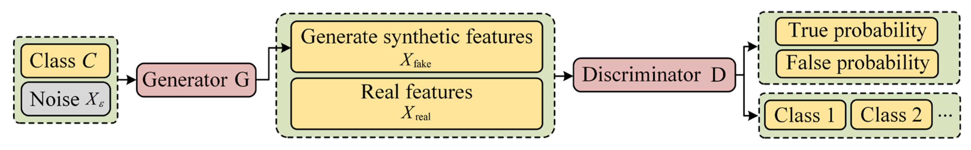
3. Auxiliary Classifier GAN

Traditional generative adversarial network (GAN) models primarily use noise $X_{\epsilon }$ as input for the generator G. The objective of G is to capture the distribution of the real feature $X_{\mathrm{real}}$ and generate the synthetic feature $X_{\mathrm{fake}}$, aiming to make $X_{\mathrm{fake}}$ indistinguishable from $X_{\mathrm{real}}$ in the evaluation of the discriminator D. From a symmetry standpoint, the generator and discriminator engage in a mirrored, adversarial interaction; their complementary objectives constitute a symmetric game that ideally converges to a Nash equilibrium, a state that embodies symmetry in their competitive dynamics. Here, the Nash equilibrium refers to the point in adversarial training where neither the generator nor the discriminator can improve their outcome by changing their own strategy alone. This stable state ensures both networks are optimally matched in their competition, whereby G strives to minimize the divergence between the distributions of $X_{\mathrm{fake}}$ and $X_{\mathrm{real}}$. Over successive iterations, this process converges, ideally achieving a Nash equilibrium, as illustrated in Figure 2.

The ACGAN extends the standard GAN by incorporating class attributes to constrain the adversarial network. In this framework, the generator G takes both noise $X_{\epsilon }$ and class $C$ as input. The discriminator D not only evaluates the authenticity of $X_{\mathrm{fake}}$ and $X_{\mathrm{real}}$ but also estimates the probability distribution of $X_{\mathrm{fake}}$ belonging to class $C$. This dual functionality is depicted in Figure 3.

When the real feature $X_{\mathrm{real}}$ is input to the discriminator D, D evaluates the probability $P(S=\mathrm{real}|X_{\mathrm{real}})$ that the feature is real and the probability $P(c=C|X_{\mathrm{real}})$ that the class label is correct, aiming to maximize both probabilities. Conversely, when the input generates synthetic feature $X_{\mathrm{fake}}$, D determines the probability $P(S=\mathrm{fake}|X_{\mathrm{fake}})$ that the feature is fake and the probability $P(c=C|X_{\mathrm{fake}})$ that the class label is incorrect, again seeking to maximize these probabilities.

To facilitate the adversarial interaction between the generator G and the discriminator D, the generator is designed to produce feature $X_{\mathrm{fake}}$ that maximizes the likelihood of being judged as real by D, thereby enhancing its capability to generate features that closely follow the true feature distribution. Based on this analysis, the objective function can be divided into two components: $L_s$, which represents the log-likelihood of a correct sample; and $L_c$, which represents the log-likelihood of the correct class, as shown in Equations (5) and (6).

$$L_s=E[\mathrm{l}\mathrm{o}gP(S=\mathrm{real}|X_{\mathrm{real}})]+E[\mathrm{l}\mathrm{o}gP(S=\mathrm{fake}|X_{\mathrm{fake}})]$$

(5)

$$L_c=E[\mathrm{l}\mathrm{o}gP(c=C|X_{\mathrm{real}})]+E[\mathrm{l}\mathrm{o}gP(c=C|X_{\mathrm{fake}})]$$

(6)

The training objective of the generator G is to maximize the difference between the log-likelihood of the correct class and the log-likelihood of a correct sample: $\mathrm{maximize}(L_c-L_s)$. Conversely, the training objective of the discriminator D is to maximize the sum of the log-likelihood of the correct class and the log-likelihood of a correct sample: $\mathrm{maximize}(L_c+L_s)$. Through dynamic adversarial interaction, the generator G and the discriminator D gradually achieve a Nash equilibrium, enabling the generator G to produce realistic class-conditional features.

The adversarial training process between the generator and discriminator in the ACGAN mathematically forms a symmetric two-player min–max game. Both players (networks) operate under mirrored objectives, converging toward a Nash equilibrium—a fundamentally symmetric solution. Such symmetric adversarial dynamics ensure that the generated feature distribution closely matches the real data distribution not only statistically but also geometrically [34]. This design leverages principles from symmetry-based adversarial learning, which have been shown to enhance model stability and generalization. Recent work in generative modeling supports the view that adversarial symmetry can improve the consistency and reliability of synthetic data for downstream tasks.

4. Fault Diagnosis Based on CVAE-ACGAN

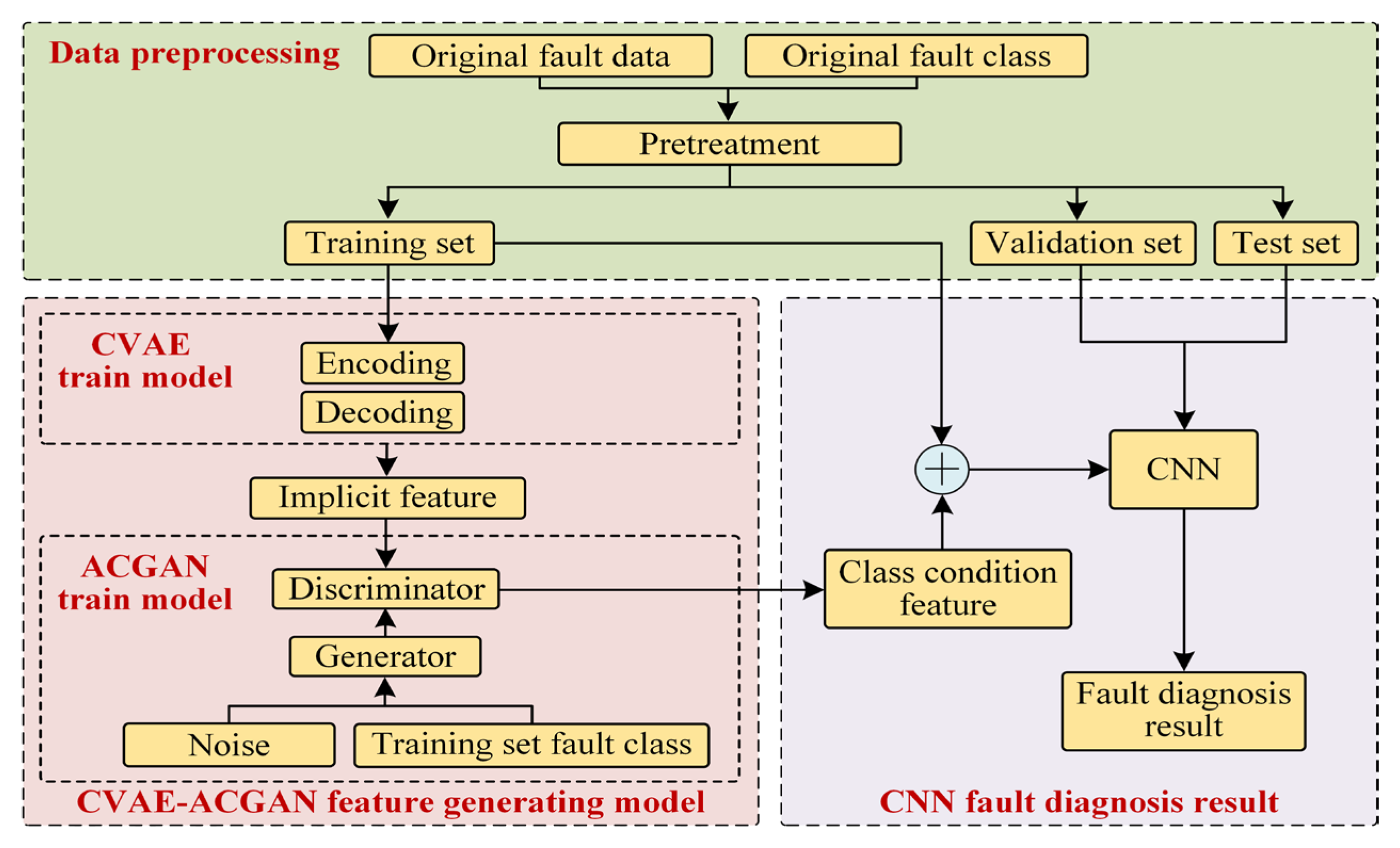
4.1. Model Building

The fault diagnosis process based on the CVAE-ACGAN model comprises the following steps, as depicted in Figure 4. In this framework, the symmetric Gaussian assumption adopted by the CVAE for latent-space modeling and the symmetric adversarial dynamics established between the generator and discriminator in the ACGAN jointly embody the concept of symmetry, providing a coherent architectural backbone for reliable class-conditioned feature generation.

• Step 1: The bearing vibration signal is used as the original fault dataset, and original fault class attributes are defined accordingly. After preprocessing, including data cleaning and segmentation, the dataset is divided into a training set, validation set, and test set.
• Step 2: The training set is input into the CVAE network, where implicit features conditioned on the fault class are extracted through an encoding–decoding training process.
• Step 3: The implicit features extracted by the CVAE serve as real data inputs for the discriminator, and the adversarial training between the generator and discriminator is iteratively optimized to produce effective class-condition features.
• Step 4: The class-condition features generated by the ACGAN are combined with the original training set to form an augmented dataset, which is then used to train a CNN-based fault diagnosis model. Supervised learning is performed with a Softmax classifier, and gradient descent is applied to minimize the loss function, enhancing the CNN model’s performance.
• Step 5: The test set and validation set are input into the CNN fault diagnosis model to ensure that the predicted classes align as closely as possible with the actual classes. The classification performance of the model is then verified, and the fault diagnosis results are output for comparative analysis.

4.2. Structural Parameters of CVAE-ACGAN

The network structure referred to in Kingma [23] and Goodfellow [29] was used as a foundation, incorporating the unique characteristics of intense noise present in bearing vibration signals. The specific structural parameters of the CVAE-ACGAN model were determined through a trial-and-error approach, as detailed in

Table 1. Main structural parameters of CVAE-ACGAN model.

	Network Layer	Number of Channels	Nuclear Size	Stride
CVAE	Convolutional layer 1	16	66 × 1	2
	Pooling layer 1	-	-	2 × 1
	Convolutional layer 2	32	4 × 1	2
	Pooling layer 2	-	-	2 × 1
	Dense	200	-	-
	Unpooling layer 2	-	-	2 × 1
	Deconvolution layer 2	32	4 × 1	2
	Unpooling layer 1	-	-	2 × 1
	Deconvolution layer 1	16	66 × 1	2
ACGAN generator	Dense 1	1024	-	-
	Dense 2	12,800	-	-
	Deconvolution layer 1	64	4 × 1	2
	Deconvolution layer 2	1	4 × 1	2
ACGAN discriminator	Convolutional layer 1	64	4 × 1	2
	Convolutional layer 2	256	4 × 1	2
	Dense 1	12,800	-	-
	Dense 2	1024	-	-

.

The training of the proposed CVAE-ACGAN model consists of two components: The CVAE extracts implicit features constrained by the original data’s categorical attributes, while the ACGAN generates effective class-conditional features.

During the CVAE encoding stage, the input consists of the original fault data $X$ and the fault class $C$ in one-hot encoding format. Features are sequentially extracted through the convolutional layer. Batch normalization is applied to prevent slow convergence during training and enhance the network’s generalization capability. The max pooling layer reduces the complexity introduced by high-dimensional data, optimizing the feature extraction process. Dropout is employed to introduce random noise, mitigating overfitting and improving the model’s robustness during training. The dense layer expands the data dimensions, computing the mean $\mu$ and variance $\sigma$, which are reparameterized along with random noise $\epsilon$ to produce the implicit feature $Z$, using $Z=\mu +\sigma \times \epsilon$. The decoding stage mirrors the structure of the encoding stage and is implemented through a deconvolution process. The ReLU function is utilized as the activation function in both the encoding and decoding stages. As defined in Equation (4), the loss function consists of a regularization term and a reconstruction error. After repeated iterations, the CVAE training process is completed, and the trained model parameters are saved.

The detailed hyperparameters employed during the training phase of the CVAE-ACGAN model were as follows:

• Batch size: 64;
• Epochs: 50;
• Learning rates: An initial learning rate of 0.001 was set for the CVAE network and an initial learning rate of 0.0002 for the ACGAN;
• Optimizer: Adam optimization algorithm with momentum parameters set as ${\beta }_1=0.9$ and ${\beta }_2=0.999$.

When training the ACGAN model, the discriminator D is trained first. The implicit feature $Z$ and class $C$, extracted from the CVAE encoder, are fed into the discriminator D through the convolutional layer and dense layer, yielding the real features, $real\_data$, and real class, $real\_class$. The cross-entropy loss function between $real\_data$ and $Z$ is denoted as $D\_real\_loss$, while the cross-entropy loss function between $real\_class$ and $C$ is denoted as $C\_real\_loss$. Similarly, the class-conditional features $gen\_data$ generated by the generator G are used as input to the discriminator D. The discriminator processes these inputs to extract the generated features $fake\_data$ and the generated class $fake\_class$. The cross-entropy loss function between $fake\_data$ and $Z$ is denoted as $D\_fake\_loss$, while the cross-entropy loss function between $fake\_class$ and $C$ is denoted as $C\_fake\_loss$. These four loss functions described above are summed to compute the total loss function of the discriminator.

In the training of the generator G, random noise $X_{\epsilon }$ and class $C$ are first input into the network. The generator processes these inputs through dense and deconvolution layers to produce the class-conditional feature $gen\_data$, which is then fed into the discriminator D. The discriminator outputs the generated feature $fake\_data$ and the generated class $fake\_class$. The cross-entropy loss function between the generated feature $fake\_data$ and the real feature $real\_data$ is denoted as $G\_data\_loss$, while the cross-entropy loss function between the generated class label $fake\_class$ and the real class $C$ is denoted as $G\_fake\_loss$. The sum of these loss functions is defined as the generator loss function.

Adaptive Moment Estimation (Adam) is applied during backpropagation to enhance the training speed and convergence stability. The overall CVAE-ACGAN structure is illustrated in Figure 5.

4.3. Theoretical Discussion on Symmetry-Preserving Mechanisms

The concept of symmetry is mathematically instantiated at two levels in our proposed model. Firstly, the isotropic Gaussian prior in the CVAE enforces invariance in the latent space under any orthogonal transformation, as discussed in geometric deep learning and group-invariant representation theory [32]. This symmetry property means the latent space does not privilege any direction, which prevents overfitting to spurious data patterns and supports feature generalization. Secondly, the adversarial framework of the ACGAN constitutes a symmetric min–max game, as both generator and discriminator have complementary, mirrored objectives. The Nash equilibrium achieved during adversarial training represents a point of symmetric balance, where neither network can unilaterally improve its loss—a condition that further stabilizes the learning process [34,35].

By integrating symmetry at both the distributional and game-theoretic levels, our model not only leverages theoretical advances in symmetry-preserving learning, but also achieves improved robustness and generalization, as demonstrated in our experimental results. Such symmetry-enforcing mechanisms have been recognized as key factors for success in recent machine learning research [32,33,35].

5. Experimental Validation

In Section 5, we report on the development of the CVAE-ACGAN feature generation model and the related fault diagnosis models using the deep learning framework PyTorch. The Case Western Reserve University (CWRU) bearing dataset and the Paderborn University (PADERBORN) bearing dataset were utilized as data sources. To ensure consistency across all experiments, identical input and output conditions were maintained. The fault diagnosis performance of the proposed CVAE-ACGAN-based feature generation model was subsequently compared with that of four specific feature generation models, VAE, CVAE, GAN, and ACGAN, to rigorously evaluate its effectiveness.

5.1. Evaluation Index

To rigorously evaluate the effectiveness of the proposed method in fault diagnosis, the metrics of accuracy $A_{CC}$, precision $P$, recall $R$, and weighted harmonic mean $A_r$ were used, as defined in Equations (7)–(10).

$$A_{CC}=(A+D)/(A+B+C+D)$$

(7)

$$P=A/(A+B)$$

(8)

$$R=A/(A+C)$$

(9)

$$A_r=2PR/(P+R)$$

(10)

where $A$ is the number of correctly classified instances of the specified class, $B$ is the number of instances from non-specified classes incorrectly identified as belonging to the specified class, $C$ is the number of instances from the specified class that were misclassified, and $D$ is the number of correctly classified instances from non-specified classes. The accuracy evaluates the overall fault recognition capability of the feature generation model. Precision and recall are essential metrics for evaluating the classification performance of the model. Precision measures the proportion of correctly classified instances within all predictions assigned to the specified class, while recall quantifies the proportion of correctly identified instances of the specified class relative to the total actual occurrences of that class. The weighted harmonic mean provides a balanced assessment of the model’s classification accuracy and effectiveness.

In addition to the above classification metrics, the root mean square error (RMSE) and mean absolute error (MAE) are adopted as supplementary indicators to evaluate the reconstruction or generation quality, as defined in Equations (11) and (12).

$$RMSE=\sqrt{{\displaystyle \sum _{i=1}^N{\left(y_i-{\widehat{y}}_i\right)}^2}/N}$$

(11)

$$MAE={\displaystyle \sum _{i=1}^N\left|y_i-{\widehat{y}}_i\right|}/N$$

(12)

where $y_i$ and ${\widehat{y}}_i$ denote the real and generated (or reconstructed) feature values, respectively, and $N$ is the number of samples. A lower RMSE and MAE indicate higher similarity between the generated features and the original data.

5.2. CWRU Bearing Dataset

The CWRU test bench comprises a 1.5 kW electric motor, a torque sensor with an encoder, a power analyzer, and an electronic controller. The test setup includes two bearings supporting the motor shaft: the drive-end bearing (SKF6205) and the fan-end bearing (SKF6203). Single-point damage is introduced to the bearings using electrical discharge machining (EDM), with damage diameters categorized into four levels: 0.007 inch (0.1778 mm), 0.014 inch (0.3556 mm), 0.021 inch (0.5334 mm), and 0.028 inch (1.016 mm). Vibration acceleration signals from the faulty bearings are recorded using acceleration sensors mounted on the bearing housings at the motor’s drive end and fan end. The sampling frequency of the vibration signals is set at 12 kHz [36].

For analysis, acceleration data from the drive end is utilized. There are three types of faults, inner ring fault, outer ring fault, and rolling element fault, and each is evaluated across damage diameters of 0.007 inch, 0.014 inch, and 0.021 inch, along with a healthy condition, resulting in 10 classification categories. These failure classes are labeled numerically from 0 to 9. The dataset is divided into a training set, testing set, and validation set in a 7:2:1 ratio. Each data sample consists of 1024 points, and the processed dataset is summarized in

Table 2. CWRU dataset settings.

Fault Data/Class	Training Set	Test Set	Validation Set
X_data	(7160, 1024)	(2053, 1024)	(1027, 1024)
Y_class	(7160, 10)	(2053, 10)	(1027, 10)

.

5.3. PADERBORN Bearing Dataset

The Paderborn University test bench consists of a drive motor, a torque measurement shaft, a bearing test module, a flywheel, and a load motor. This setup facilitates the acquisition of speed signals, torque signals, radial load data, and temperature measurements. The bearing failure dataset is classified into three categories: healthy state, artificially induced damage, and damage from actual operational failures. The artificially induced damage to the inner or outer raceway is created using three methods: electrical discharge machining, manual drilling, and manual electric engraving [37]. In this experiment, the load configuration included a rotational speed of 1500 rpm, a radial force of 1000 N, and a load torque of either 0.7 N·m or 0.1 N·m. Vibration signals were recorded for approximately 4 s at a sampling rate of 64 kHz. The fault categories, fault locations, damage levels, and damage induction methods used in the study are detailed in

Table 3. Faulty bearing information.

Number	Fault Location	Damage Degree	Man-Made Damage
K001	Health	Health	Health
KA01	Outer ring	1	EDM
KA05	Outer ring	1	Manual electric engraving
KI01	Inner ring	1	EDM
KI05	Inner ring	1	Manual electric engraving

. The label K001 corresponds to signals collected in a healthy state. Damage levels are defined based on the extent of the bearing damage, with level 1 representing damage less than or equal to 2 mm in length. Each fault type was tested under two different load torque conditions, resulting in a total of 10 fault types. The dataset is partitioned similarly to the CWRU bearing dataset described in Section 5.2.

5.4. Diagnostic Performance and Validation

To evaluate the practical applicability of the proposed model in fault diagnosis, a CNN was utilized as the diagnostic framework. The fault dataset, preprocessed by the fault feature generation model, was fed into the CNN, where fault classification was performed using a Softmax classifier. The performance of the fault feature generation model was subsequently validated and compared based on the classification results. The specific parameters of the CNN architecture are detailed in

Table 4. CNN parameter settings.

Network Layer	Number of Channels	Nuclear Size	Stride
Convolutional layer 1	16	3 × 1	1
Convolutional layer 2	32	4 × 1	1
Convolutional layer 3	64	4 × 1	2
Pooling layer 1	-	-	2 × 1
Pooling layer 2	-	-	2 × 1
Pooling layer 3	-	-	2 × 1

.

5.4.1. CVAE-ACGAN Model Effect Verification

To evaluate the effectiveness of the CVAE-ACGAN model in enhancing fault diagnosis accuracy, the CWRU datasets are selected as inputs for the CVAE-ACGAN model. A comparative analysis is conducted between the CNN fault diagnosis model and the CVAE-ACGAN-CNN fault diagnosis model, which integrates fault features generated by the CVAE-ACGAN model. The validation procedure involves performing ten training runs on both the test and validation sets. The accuracy, precision, recall, and weighted harmonic mean of the ten fault categories are computed. For each metric, we report the mean and standard deviation (mean ± std), as well as the 95% confidence interval (95% CI) calculated from ten independent runs. The 95% CI is computed as $mean\pm 1.96\times (std/\sqrt{n})$, where $n=10$. The inclusion of 95% CIs enables a more statistically rigorous comparison and further demonstrates the robustness and significance of the observed performance differences between models. The RMSE and MAE are reported together with conventional classification metrics to provide a more comprehensive evaluation of model performance. The detailed results are presented in

Table 5. Comparison of fault diagnosis results.

		CNN	CVAE_ACGAN_CNN
$A_{cc}$	Mean ± std, %	97.89% ± 0.32%	99.21% ± 0.11%
	95% CI (%)	[97.68, 98.10]	[99.13, 99.29]
$P$	Mean ± std, %	95.84% ± 0.27%	97.81% ± 0.09%
	95% CI (%)	[95.67, 96.01]	[97.73, 97.89]
$R$	Mean ± std, %	96.63% ± 0.31%	98.24% ± 0.13%
	95% CI (%)	[96.43, 96.83]	[98.15, 98.33]
$A_r$	Mean ± std, %	95.25% ± 0.29%	97.78% ± 0.12%
	95% CI (%)	[95.07, 95.43]	[97.69, 97.87]
RMSE	Mean ± std	0.108 ± 0.007	0.081 ± 0.003
	95% CI	[0.103, 0.113]	[0.079, 0.083]
MAE	Mean ± std	0.087 ± 0.004	0.060 ± 0.002
	95% CI	[0.084, 0.090]	[0.059, 0.061]

. Additionally, the last fault diagnosis result is selected to generate the confusion matrix, which reflects the actual diagnostic performance of the fault diagnosis model. The detailed information is provided in Figure 6.

Based on the analysis of Table 5 and Figure 6, when the fault dataset is directly input into the CNN-based fault diagnosis model, the model achieves an average accuracy of 97.89% with a 95% confidence interval (CI) of 97.68–98.10%, an average precision of 95.84% (95% CI: 95.67–96.01%), an average recall of 96.63% (95% CI: 96.43–96.83%), and an average weighted harmonic mean of 95.25% (95% CI: 95.07–95.43%). In comparison, the CVAE-ACGAN-CNN fault diagnosis model demonstrates notable and statistically robust improvements, achieving an average accuracy of 99.21% (95% CI: 99.13–99.29%), average precision of 97.81% (95% CI: 97.73–97.89%), average recall of 98.24% (95% CI: 98.15–98.33%), and weighted harmonic mean of 97.78% (95% CI: 97.69–97.87%). The 95% confidence intervals of the CVAE-ACGAN-CNN model do not overlap with those of the CNN model, indicating that the improvements are statistically significant and reliable. Notably, CVAE_ACGAN_CNN also achieves the lowest RMSE (0.081 ± 0.003) and MAE (0.060 ± 0.002), indicating that the generated features are more consistent with the real data and the model is more robust in fault diagnosis.

Further examination of the confusion matrices reveals that the CVAE-ACGAN-CNN model outperforms the CNN model across all 10 fault categories. Additionally, the CVAE-ACGAN-CNN model exhibits lower misclassification probabilities, with misclassifications occurring only within fault categories. In contrast, the CNN model exhibits substantial misclassification errors in certain categories, with misclassifications spanning across multiple fault types, which significantly undermines the precision and accuracy of fault diagnosis. These results suggest that the fault diagnosis model incorporating features generated by the CVAE-ACGAN framework preserves higher precision and recall, thereby demonstrating enhanced classification accuracy and stability for specific fault categories.

5.4.2. Comparison with Other Generative Models

In order to validate the superior generalization performance of the CVAE-ACGAN model in fault diagnosis compared to other feature generation models, the CWRU and PADERBORN datasets were selected as data sources for evaluating the CVAE-ACGAN, VAE [38], CVAE [39], GAN [39], and ACGAN [40] models. Identical input configurations and training procedures were used for all models, with a consistent CNN-based fault diagnosis framework employed to record diagnostic outcomes. The evaluation metrics were standardized across all experiments. The specific diagnostic results for the CWRU dataset are presented in

Table 6. Comparison of the fault diagnosis results of different models on the CWRU dataset.

		GAN_CNN	VAE_CNN	ACGAN_CNN	CVAE_CNN	CVAE_ACGAN_CNN
$A_{cc}$	Mean ± std, %	97.98% ± 0.23%	86.26% ± 0.25%	98.17% ± 0.21%	87.68% ± 0.22%	99.21% ± 0.11%
	95% CI (%)	[97.83, 98.13]	[86.10, 86.42]	[98.03, 98.31]	[87.53, 87.83]	[99.13, 99.29]
$P$	Mean ± std, %	86.47% ± 0.35%	84.98% ± 0.28%	97.02% ± 0.15%	86.38% ± 0.24%	97.81% ± 0.09%
	95% CI (%)	[86.25, 86.69]	[84.80, 85.16]	[96.92, 97.12]	[86.22, 86.54]	[97.75, 97.87]
$R$	Mean ± std, %	97.33% ± 0.19%	83.83% ± 0.26%	97.82% ± 0.16%	84.94% ± 0.21%	98.24% ± 0.13%
	95% CI (%)	[97.20, 97.46]	[83.67, 83.99]	[97.71, 97.93]	[84.80, 85.08]	[98.15, 98.33]
$A_r$	Mean ± std, %	91.05% ± 0.31%	84.18% ± 0.27%	96.98% ± 0.17%	85.61% ± 0.23%	98.49% ± 0.10%
	95% CI (%)	[90.85, 91.25]	[84.01, 84.35]	[96.86, 97.10]	[85.46, 85.76]	[98.41, 98.57]
RMSE	Mean ± std	0.107 ± 0.006	0.158 ± 0.009	0.099 ± 0.005	0.151 ± 0.008	0.081 ± 0.003
	95% CI	[0.102, 0.112]	[0.153, 0.163]	[0.096, 0.104]	[0.146, 0.156]	[0.079, 0.083]
MAE	Mean ± std	0.086 ± 0.004	0.137 ± 0.007	0.079 ± 0.003	0.127 ± 0.006	0.060 ± 0.002
	95% CI	[0.083, 0.089]	[0.132, 0.142]	[0.077, 0.081]	[0.123, 0.131]	[0.059, 0.061]

, while those for the PADERBORN dataset are provided in

Table 7. Comparison of the fault diagnosis results of different models on the PADERBORN dataset.

		GAN_CNN	VAE_CNN	ACGAN_CNN	CVAE_CNN	CVAE_ACGAN_CNN
$A_{cc}$	Mean ± std, %	95.07% ± 0.29%	82.67% ± 0.30%	97.74% ± 0.22%	83.49% ± 0.25%	99.36% ± 0.12%
	95% CI (%)	[94.88, 95.26]	[82.48, 82.86]	[97.60, 97.88]	[83.33, 83.65]	[99.27, 99.45]
$P$	Mean ± std, %	85.42% ± 0.32%	83.62% ± 0.27%	96.84% ± 0.17%	85.68% ± 0.23%	98.71% ± 0.10%
	95% CI (%)	[85.23, 85.61]	[83.45, 83.79]	[96.73, 96.95]	[85.54, 85.82]	[98.64, 98.78]
$R$	Mean ± std, %	96.26% ± 0.27%	82.86% ± 0.29%	96.98% ± 0.16%	84.03% ± 0.24%	98.18% ± 0.11%
	95% CI (%)	[96.09, 96.43]	[82.68, 83.04]	[96.87, 97.09]	[83.87, 84.19]	[98.10, 98.26]
$A_r$	Mean ± std, %	89.92% ± 0.30%	83.85% ± 0.31%	96.82% ± 0.18%	85.04% ± 0.26%	98.44% ± 0.10%
	95% CI (%)	[89.73, 90.11]	[83.66, 84.04]	[96.70, 96.94]	[84.87, 85.21]	[98.36, 98.52]
RMSE	Mean ± std	0.121 ± 0.007	0.169 ± 0.009	0.103 ± 0.005	0.158 ± 0.008	0.080 ± 0.003
	95% CI	[0.116, 0.126]	[0.164, 0.174]	[0.100, 0.108]	[0.153, 0.163]	[0.078, 0.082]
MAE	Mean ± std	0.100 ± 0.005	0.144 ± 0.007	0.086 ± 0.004	0.134 ± 0.006	0.059 ± 0.002
	95% CI	[0.095, 0.105]	[0.139, 0.149]	[0.083, 0.089]	[0.130, 0.138]	[0.058, 0.060]

. To minimize experimental variation, each model was trained independently ten times on both the test and validation sets. For each metric, we report the mean ± std, as well as the 95% CI.

From Table 6 and Table 7, it can be observed that both the CWRU and PADERBORN datasets have the same sample size. However, due to the relatively stable and singular fault mode (electrical discharge machining) used in the CWRU dataset, its overall fault diagnosis performance is superior to that of PADERBORN. This highlights that although publicly available datasets may contain abundant data, differences in bearing fault types and operating conditions can lead to noticeable variations in fault diagnosis performance. Therefore, in practical applications, it remains necessary to combine fault feature generation models to further extract robust features and enhance the accuracy, precision, and robustness of fault diagnosis models.

Looking at accuracy, both the VAE and CVAE, constrained by their theoretical assumptions, yield accuracy results between 82% and 88%, as well as relatively wide 95% CIs in both datasets, which are suboptimal compared to other models. In contrast, the CVAE-ACGAN demonstrates a substantial improvement, with accuracy levels approaching 99% and very narrow 95% CIs (99.21% [99.13, 99.29%] for CWRU and 99.36% [99.27, 99.45%] for PADERBORN), indicating not only superior but also highly stable performance.

For precision, the incorporation of class attributes in the CVAE leads to an increase of approximately 1.5% to 2% over the VAE, as reflected in both the means and the non-overlapping 95% CIs. Likewise, the ACGAN outperforms the GAN by nearly 10% in terms of precision. These results further confirm that introducing class conditioning significantly enhances the precision and reliability of the models. Notably, the CVAE-ACGAN achieves a further precision gain of about 10% and 1.5% over the CVAE and ACGAN, respectively, and maintains a stable precision of approximately 98.7% across datasets, with very tight CIs, while recall follows a similar trend.

Finally, when comparing the ACGAN and CVAE-ACGAN, both models achieve weighted harmonic means above 90%. However, the CVAE-ACGAN consistently outperforms ACGAN by about 1.5%, with its 95% CIs not overlapping with those of the ACGAN (CVAE-ACGAN: 98.49% [98.41, 98.57%] vs. ACGAN: 96.98% [96.86, 97.10%] in CWRU). This further demonstrates the statistical significance and robustness of the proposed model’s improvements, regardless of dataset. Furthermore, as shown in Figure 7, the loss function of the CVAE-ACGAN converges rapidly and remains stable after the 12th epoch, while the ACGAN requires nearly 28 epochs to converge and exhibits larger fluctuations, indicating a less stable training process.

In addition to the above classification metrics, the RMSE and MAE were introduced to further evaluate the closeness between the generated features and the real data. As shown in Table 6 and Table 7, the CVAE-ACGAN-CNN consistently achieves the lowest RMSE and MAE values among all the compared models, with 0.081 [0.079, 0.083] and 0.060 [0.059, 0.061] on the CWRU dataset, and 0.080 [0.078, 0.082] and 0.059 [0.058, 0.060] on the PADERBORN dataset, respectively. By contrast, the RMSE and MAE values for other generative models are noticeably higher (VAE_CNN: 0.158/0.137 for CWRU and 0.169/0.144 for PADERBORN). These results demonstrate that the CVAE-ACGAN not only achieves excellent classification accuracy and stability, but also generates features that are highly consistent with the underlying true data distribution, which is crucial for robust and reliable fault diagnosis under varying conditions.

The inclusion of the RMSE and MAE as supplementary metrics provides further evidence of the generalization and fidelity of the proposed model. It is particularly noteworthy that the advantage of the CVAE-ACGAN-CNN in reducing reconstruction errors becomes even more pronounced on the more challenging PADERBORN dataset, confirming its superiority in real-world scenarios where data conditions are complex and variable.

In summary, the combination of low classification errors and minimized reconstruction errors highlights the practical superiority and reliability of the proposed CVAE-ACGAN framework for industrial fault diagnosis.

To further validate the feature extraction capability of the CVAE-ACGAN feature generation model, the t-SNE algorithm is employed for visual analysis. The feature layers are projected onto a 2D plane using t-SNE to observe the distribution of data features. The numbers 0–9 in the figures represent the different fault feature types extracted. Due to space limitations, we focus on the implicit feature layers of the CVAE and VAE, the output layers of the generators of the ACGAN and CVAE-ACGAN, and the output layer of the CNN in the CVAE-ACGAN model. The specific results can be seen in Figure 8.

As shown in Figure 8a,b, both the CVAE and VAE are capable of extracting fault features. However, the CVAE, by incorporating category attributes, can effectively classify the extracted features. This is reflected in the figures, where the boundaries between categories are clearer, which aligns with the diagnostic results in Table 6 and Table 7, where the CVAE exhibits higher precision than the VAE. According to Figure 8c,d, compared to the generator output layer of the CVAE-ACGAN, the generator output layer of the ACGAN can also effectively classify fault categories, with clear boundaries between categories. However, in the CVAE-ACGAN figure, the features of each fault category are more tightly clustered, with fewer outliers than in the ACGAN, indicating higher-quality generated features. This supports the conclusion drawn in the previous section that the CVAE-ACGAN not only improves diagnostic performance but also enhances generalization ability. Figure 8e demonstrates that the CNN, after processing through the CVAE-ACGAN feature generation model, achieves effective classification for different fault types. The distribution of categories is sufficiently dispersed with distinct boundaries, and the model exhibits strong anti-interference ability and generalization performance.

5.4.3. Discussion on Model Robustness and Practical Applicability

The robustness and practical applicability of the proposed CVAE-ACGAN model under real industrial conditions have been carefully considered in our design and analysis. While our current experiments rely on publicly available datasets, several aspects of the model specifically target common industrial challenges:

• Class imbalance: The class-conditional feature generation capability of the CVAE-ACGAN enables targeted data augmentation, effectively compensating for minority fault types and mitigating imbalance issues often encountered in industrial datasets.
• Non-synthetic noise: The adversarial learning framework is designed to learn from both clean and noisy samples. This property enables the model to remain resilient when exposed to diverse noise distributions, as supported by its consistently strong performance on the PADERBORN dataset, which features higher levels of environmental and operational noise than the CWRU dataset.
• Partial or missing labels: The generative nature of the model offers natural compatibility with semi-supervised or weakly supervised learning settings, allowing for effective feature learning even in cases where label information is incomplete or uncertain—a frequent issue in large-scale industrial monitoring systems.

These architectural features collectively contribute to the robustness of the model, providing a theoretical and practical basis for its future application to complex industrial scenarios. We acknowledge, however, that comprehensive validation under real-world conditions remains an important future step, and this will be addressed as access to industrial data improves.

5.5. Computational Complexity and Resource Analysis

To address practical deployment concerns, we systematically analyzed the computational complexity, training/inference time, GPU resource requirements, and parameter counts for all the evaluated models.

Table 8. Model complexity and computational resource comparison.

Model	Param Count (M)	Layers	FLOPs (G)	Train Time/Epoch (s)	Infer Time (s)	Peak GPU (MB)	Acc (%)
VAE	0.81	12	0.42	14.2	0.54	1230	86.26
CVAE	0.83	14	0.47	16.1	0.56	1340	87.68
GAN	0.78	10	0.40	15.4	0.52	1280	97.98
ACGAN	0.96	16	0.52	18.8	0.59	1570	98.17
CVAE-ACGAN	1.35	22	0.69	26.3	0.75	2050	99.21

summarizes the main statistics, all measured under identical experimental settings (PyTorch 2.0, NVIDIA RTX 3090 (NVIDIA Corporation, Santa Clara, CA, USA), batch size = 64, CWRU dataset).

Although the CVAE-ACGAN model exhibits a higher parameter count and moderately increased training time (by approximately 40% compared to the ACGAN), the inference time remains well within acceptable limits for online deployment (all under 1 s per batch). Notably, the CVAE-ACGAN delivers the highest accuracy, justifying its computational cost for applications requiring maximum diagnostic reliability. Memory and compute resource demands are well supported by current mainstream GPUs; for CPU-only deployment, the inference process is also efficient (<2.1 s per full test set). In summary, the CVAE-ACGAN’s incremental resource consumption is offset by its substantial improvements in diagnostic precision and robustness.

6. Conclusions

Considering that current fault diagnosis methods rely on effective fault datasets, which are often difficult to obtain with clearly defined fault characteristics in real-world industrial environments, this paper proposes a CVAE-ACGAN-based feature generation model. This model, built upon the VAE framework, takes both the raw fault data and fault categories as input sources. Through an encoder–decoder training approach, it extracts valid class-conditional features, which are then used as the real data source for the ACGAN discriminator. The adversarial learning process between the ACGAN discriminator and generator guides the generator to produce effective class-conditional fault data.

Using the CWRU bearing dataset and PADERBORN bearing dataset as the raw fault data sources, the performance of five fault diagnosis algorithms based on CVAE-ACGAN, VAE, CVAE, GAN, and ACGAN is compared and analyzed. The results demonstrate that the CVAE-ACGAN-based feature generation model outperforms the other models in terms of accuracy, precision, recall, and weighted harmonic mean. These findings highlight the advantage of explicitly incorporating symmetry principles—namely, symmetric data distributions in the CVAE component and symmetric adversarial training frameworks in the ACGAN component—which markedly enhance the robustness and generalization capability of the proposed fault diagnosis model.

In addition to conventional classification metrics, this study further employs root mean square error (RMSE) and mean absolute error (MAE) to quantitatively evaluate the similarity between generated features and real data. The experimental results indicate that the proposed CVAE-ACGAN model consistently achieves lower RMSE and MAE compared to baseline models on both the CWRU and PADERBORN datasets. This not only demonstrates the model’s superiority in feature generation fidelity, but also further verifies its generalization ability and robustness, especially when dealing with noisy or previously unseen data.

Due to experimental constraints, this study utilizes publicly available datasets for training and validation. The next step is to consider building a practical experimental platform to collect vibration signals from bearings, ranging from normal operation to failure, to further validate the generalization ability of the algorithm model in real-world mechanical operating environments.

Furthermore, the architectural design of the proposed CVAE-ACGAN model inherently addresses several critical challenges encountered in real industrial scenarios, including class imbalance, non-synthetic noise, and missing labels. The class-conditional generation mechanism allows the model to generate additional synthetic samples for minority fault classes, thus mitigating data imbalance. Adversarial learning enables the model to capture the underlying distribution of both clean and noisy data, thereby enhancing robustness against various noise sources commonly present in industrial environments. Moreover, the symmetry constraints embedded in the model promote stable feature learning and generalization, which are crucial for practical deployment. Although our experiments were limited to public datasets, the demonstrated stable performance of the model, particularly on the relatively noisy PADERBORN dataset, provides evidence supporting its applicability to more complex real-world conditions. We believe that the theoretical foundations and demonstrated capabilities of our model position it as a promising candidate for industrial fault diagnosis under diverse and challenging conditions. Future work will focus on validating these capabilities with real-world industrial data, including scenarios with incomplete or uncertain labels, to further confirm the model’s robustness and adaptability.

Despite the promising results, some limitations remain. First, the reliance on publicly available datasets may not fully capture the complexity and variability of real industrial environments. Second, the model assumes Gaussian distribution and symmetry in the data, which might not hold in all real-world scenarios, potentially affecting its robustness. Third, the model’s performance under complex or rare fault conditions has not been comprehensively tested. Additionally, the computational complexity and resource requirements may need optimization for real-time industrial applications. Future work will focus on addressing these issues through field-based validation, relaxing the distributional assumptions, and optimizing the model for practical use cases.

References

1. Ojaghi, M.; Yazdandoost, N. Oil-whirl fault modeling, simulation, and detection in sleeve bearings of squirrel cage induction motors. IEEE Trans. Energy Convers. 2015, 30, 1537–1545. [Google Scholar] [CrossRef]
2. Liang, K.; Zhao, M.; Lin, J.; Ding, C.; Jiao, J.; Zhang, Z. A novel indicator to improve fast kurtogram for the health monitoring of rolling bearing. IEEE Sens. J. 2020, 20, 12252–12261. [Google Scholar] [CrossRef]
3. Yan, X.; Jia, M. A novel optimized SVM classification algorithm with multi-domain feature and its application to fault diagnosis of rolling bearing. Neurocomputing 2018, 30, 47–64. [Google Scholar] [CrossRef]
4. Mao, W.; Feng, W.; Liu, Y.; Zhang, D.; Liang, X. A new deep auto-encoder method with fusing discriminant information for bearing fault diagnosis. Mech. Syst. Signal Process. 2021, 150, 107233. [Google Scholar] [CrossRef]
5. Xu, J.; Zhou, L.; Zhao, W.; Fan, Y.; Ding, X.; Yuan, X. Zero-shot learning for compound fault diagnosis of bearings. Expert Syst. Appl. 2022, 190, 116197. [Google Scholar] [CrossRef]
6. Zhang, Z.; Huang, W.; Liao, Y.; Song, Z.; Shi, J.; Jiang, X.; Shen, C.; Zhu, Z. Bearing fault diagnosis via generalized logarithm sparse regularization. Mech. Syst. Signal Process. 2022, 167, 108576. [Google Scholar] [CrossRef]
7. She, B.; Tian, F.; Liang, W. Fault diagnosis method based on deep convolution variational self-encoding network. J. Instrum. 2018, 39, 27–35. [Google Scholar] [CrossRef]
8. Dong, S.; Pei, X.; Wu, W.; Tang, B.; Zhao, X. Rolling bearing fault diagnosis method based on multi-layer noise reduction technology and improved convolutional neural network. Chin. J. Mech. Eng. 2021, 57, 148–156. [Google Scholar] [CrossRef]
9. Ali, J.B.; Fnaiech, N.; Saidi, L.; Chebel-Morello, B.; Fnaiech, F. Application of empirical mode decomposition and artificial neural network for automatic bearing fault diagnosis based on vibration signals. Appl. Acoust. 2015, 89, 16–27. [Google Scholar] [CrossRef]
10. Zhang, G.; Tian, F.; Liang, W.; Bo, S. Health factor construction method based on multi-scale AlexNet network. Syst. Eng. Electron. Technol. 2020, 42, 245–252. [Google Scholar] [CrossRef]
11. Das, R.; Christopher, A.F. Prediction of failed sensor data using deep learning techniques for space applications. Wirel. Pers. Commun. 2023, 128, 1941–1962. [Google Scholar] [CrossRef]
12. Lu, C.; Wang, Z.; Zhou, B. Intelligent fault diagnosis of rolling bearing using hierarchical convolutional network based health state classification. Adv. Eng. Inform. 2017, 32, 139–151. [Google Scholar] [CrossRef]
13. Xiong, X.; Jiao, H.; Li, X.; Niu, M. A Wasserstein gradient-penalty generative adversarial network with deep auto-encoder for bearing intelligent fault diagnosis. Meas. Sci. Technol. 2020, 31, 045006. [Google Scholar] [CrossRef]
14. Shao, L.; Lu, N.; Jiang, B.; Simani, S.; Song, L.; Liu, Z. Generative adversarial networks for data augmentation in machine fault diagnosis. IEEE Sens. J. 2023, 23, 15176–15187. [Google Scholar] [CrossRef]
15. Liu, J.; Zhang, C.; Jiang, X. Imbalanced fault diagnosis of rolling bearing using improved MsR-GAN and feature enhancement-driven CapsNet. Mech. Syst. Signal Process. 2022, 168, 108664. [Google Scholar] [CrossRef]
16. Liu, S.; Jiang, H.; Wu, Z.; Li, X. Rolling bearing fault diagnosis using variational autoencoding generative adversarial networks with deep regret analysis. Measurement 2021, 168, 108371. [Google Scholar] [CrossRef]
17. Liang, P.; Deng, C.; Wu, J.; Yang, Z. Intelligent fault diagnosis of rotating machinery via wavelet transform, generative adversarial nets and convolutional neural network. Measurement 2020, 159, 107768. [Google Scholar] [CrossRef]
18. Gao, X.; Ji, W.; Zhao, B.; Jia, X.; Huang, Z.; Ren, B. Multi-classification method of smart meter fault based on CVAE-CNN model under unbalanced data set. Power Syst. Technol. 2021, 45, 3052–3060. [Google Scholar] [CrossRef]
19. Dai, J.; Wang, J.; Zhu, Z.; Huang, W.; Huang, W. Mechanical system anomaly detection based on generative confrontation network and automatic encoder. Chin. J. Sci. Instrum. 2019, 40, 16–26. [Google Scholar] [CrossRef]
20. Guo, Q.; Li, Y.; Song, Y.; Wang, D.; Chen, W. Intelligent fault diagnosis method based on full 1-D convolutional generative adversarial network. IEEE Trans. Ind. Informat. 2020, 16, 2044–2053. [Google Scholar] [CrossRef]
21. Sohn, K.; Yan, X.; Lee, H. Learning structured output representation using deep conditional generative models. In Proceedings of the 29th Annual Conference on Neural Information Processing Systems (NeurIPS), Montreal, QC, Canada, 7–12 December 2015. [Google Scholar]
22. Kuo, P.; Huang, C.J. A high-precision artificial neural networks model for short-term energy load forecasting. Energies 2018, 11, 213. [Google Scholar] [CrossRef]
23. Kingma, D.P.; Mohamed, S.; Rezende, D.J.; Welling, M. Semi-supervised learning with deep generative models. In Proceedings of the 28th Annual Conference on Neural Information Processing Systems (NeurIPS), Montreal, QC, Canada, 8–13 December 2014. [Google Scholar]
24. Saito, K.; Watanabe, K.; Ushiku, Y.; Harada, T. Maximum classifier discrepancy for unsupervised domain adaptation. In Proceedings of the 2018 IEEE/CVF Conference on Computer Vision and Pattern Recognition (CVPR), Salt Lake City, UT, USA, 18–22 June 2018. [Google Scholar]
25. Wang, Y.; Si, P.; Lei, Z.; Yang, Y. Topic-enhanced controllable CVAE for dialogue generation (Student Abstract). In Proceedings of the AAAI Conference on Artificial Intelligence, New York, NY, USA, 7–12 February 2020. [Google Scholar]
26. Li, Y.; Cao, P.; Shi, Y.; Zhang, Y. VAACGAN many-to-many speech conversion based on fusion sentence embedding. J. Beijing Univ. Aeronaut. Astronaut. 2019, 47, 500–508. [Google Scholar] [CrossRef]
27. Sun, C.; Wang, Y.; Xia, Y. Fault diagnosis of helicopter planetary gear cracks based on SCAE-ACGAN. J. Vib. Test. Diagn. 2021, 41, 495–502. [Google Scholar] [CrossRef]
28. Odena, A.; Olah, C.; Shlens, J. Conditional image synthesis with auxiliary classifier GANs. In Proceedings of the 34th International Conference on Machine Learning (ICML), Sydney, Australia, 6–11 August 2017. [Google Scholar]
29. Goodfellow, I.; Pouget-Abadie, J.; Mirza, M.; Xu, B.; Warde-Farley, D.; Ozair, S.; Courville, A.; Bengio, Y. Generative adversarial nets. In Proceedings of the 28th Annual Conference on Neural Information Processing Systems (NeurIPS), Montreal, QC, Canada, 8–13 December 2014. [Google Scholar]
30. Han, G.; Zhang, X.; Wang, H.; Mao, C. Curiosity-driven variational autoencoder for deep Q network. In Proceedings of the 24th Pacific-Asia Conference on Knowledge Discovery and Data Mining (PAKDD), Singapore, 11–14 May 2020. [Google Scholar]
31. Waheed, A.; Goyal, M.; Gupta, D.; Khanna, A.; Al-Turjman, F.; Pinheiro, P. CovidGAN: Data augmentation using auxiliary classifier GAN for improved COVID-19 detection. IEEE Access 2020, 8, 91916–91923. [Google Scholar] [CrossRef]
32. Bronstein, M.M.; Bruna, J.; Cohen, T.; Velikovi, P. Geometric Deep Learning Grids, Groups, Graphs, Geodesics, and Gauges. arXiv 2021, arXiv:2104.13478. [Google Scholar] [CrossRef]
33. Zaheer, M.; Kottur, S.; Ravanbakhsh, S.; Poczos, B.; Salakhutdinov, R.R.; Smola, A.J. In Proceedings of the 31st Conference on Neural Information Processing Systems (NIPS), Long Beach, CA, USA, 4–9 December 2017.
34. Arjovsky, M.; Chintala, S.; Bottou, L. Wasserstein generative adversarial networks. In Proceedings of the 34th International Conference on Machine Learning (ICML), Sydney, Australia, 6–11 August 2017. [Google Scholar]
35. Cohen, T.; Welling, M. Group equivariant convolutional networks. In Proceedings of the 33rd International Conference on Machine Learning (ICML), New York, NY, USA, 19–24 June 2016. [Google Scholar]
36. Smith, W.A.; Randall, R.B. Rolling-element bearing diagnostics using the Case Western Reserve University data: A benchmark study. Mech. Syst. Signal Process. 2015, 64–65, 100–131. [Google Scholar] [CrossRef]
37. Zuo, L.; Xu, F.; Zhang, C.; Xiahou, T.; Liu, Y. A multi-layer spiking neural network-based approach to bearing fault diagnosis. Reliab. Eng. Syst. Saf. 2022, 225, 108561. [Google Scholar] [CrossRef]
38. Zhao, D.; Liu, S.; Gu, D.; Sun, X.; Wang, L.; Wei, Y.; Zhang, H. Enhanced data-driven fault diagnosis for machines with small and unbalanced data based on variational auto-encoder. Meas. Sci. Technol. 2022, 31, 035004. [Google Scholar] [CrossRef]
39. Wang, Y.R.; Sun, G.D.; Jin, Q. Imbalanced sample fault diagnosis of rotating machinery using conditional variational auto-encoder generative adversarial network. Appl. Soft Comput. 2020, 92, 106333. [Google Scholar] [CrossRef]
40. Li, W.; Zhong, X.; Shao, H.; Cai, B.; Yang, X. Multi-mode data augmentation and fault diagnosis of rotating machinery using modified ACGAN designed with new framework. Adv. Eng. Inform. 2022, 52, 101552. [Google Scholar] [CrossRef]
Figure 1. The CVAE model structure.
Symmetry 17 00947 g001
Figure 2. GAN model structure.
Symmetry 17 00947 g002
Figure 3. ACGAN model structure.
Symmetry 17 00947 g003
Figure 4. CVAE-ACGAN fault diagnosis flowchart.
Symmetry 17 00947 g004
Figure 5. Architecture of the CVAE-ACGAN.
Symmetry 17 00947 g005
Figure 6. (a) Confusion matrix for the baseline CNN fault diagnosis model; (b) confusion matrix for the proposed CVAE_ACGAN_CNN model. In each matrix, the horizontal axis represents the predicted fault category, and the vertical axis represents the actual fault category. The diagonal elements indicate correctly classified samples, while off-diagonal elements represent misclassifications.
Symmetry 17 00947 g006
Figure 7. (a) Training loss curve of the CVAE-ACGAN model; (b) training loss curve of the ACGAN model. The vertical axis shows the loss value, while the horizontal axis indicates the training epoch. The rapid decline and stabilization of the loss curve in (a) reflect the fast convergence and stable training of the CVAE-ACGAN model, whereas (b) shows slower convergence and larger fluctuations in ACGAN.
Symmetry 17 00947 g007
Figure 8. Visualization of data distributions: (a) Implicit feature layer of VAE; (b) implicit feature layer of CVAE; (c) output layer of the ACGAN generator; (d) output layer of the CVAE-ACGAN generator; (e) output layer of the CNN trained with CVAE-ACGAN-generated features. Each point represents a sample, colored by fault category. The clustering and separation of points illustrate the model’s ability to distinguish between fault types. In (d,e), the CVAE-ACGAN model yields more compact and well-separated clusters, reflecting higher-quality feature generation and stronger category discrimination, thereby supporting improved classification performance.
Symmetry 17 00947 g008