Sequential Fusion Least Squares Method for State Estimation of Multi-Sensor Linear Systems Under Noise Cross-Correlation

Abstract

This paper investigates a multi-sensor system for the state estimation of a maneuvering target, wherein the process noise of the target dynamics and the measurement noise of the sensor network are mutually correlated, and the measurement noises across different sensors are also cross-correlated. Under such conditions, we propose a globally optimal sequential least squares fusion estimation algorithm within the framework of linear minimum mean square error (LMMSE) estimation. This method is specifically designed to preserve structural symmetry and to accommodate the time-ordered arrival of sensor observations transmitted over a network. Rigorous theoretical analysis establishes the performance equivalence between the proposed sequential fusion estimator and the centralized Kalman filter. Numerical simulations further demonstrate the algorithm’s superior estimation accuracy and stability under symmetry constraints, particularly when the noise statistics exhibit spatial or temporal symmetry.

1. Introduction

State estimation (or filtering) is one of the most important research areas in the operation of industrial systems [1]. It refers to the process of describing the internal state structure of a system based on external observed output data. Over the past few decades, state estimation problems have been present in nearly all fields, including industry, the military, and finance. They have been widely applied in areas such as autonomous driving [2], parameter estimation [3], system identification [4], target tracking, and aerospace [5]. Parameter identification has also found extensive applications across various fields, such as parameter updating in control systems, parameter estimation in communication systems, and fault diagnosis in power systems [6]. With technological advancements, multi-sensor systems have become increasingly prevalent. Multi-sensor information fusion, also known as multi-source information fusion, refers to the process of optimally combining data from single or multiple sources to obtain accurate and reliable information. This approach has been widely applied in numerous high-profile and emerging fields, including industrial process monitoring, inertial navigation, industrial robotics, unmanned systems [7], the Internet of Things (IoT) [8], electric motor and appliance design, and air traffic control systems [9]. By fusing data from multiple sensors, the resulting estimates are more accurate, the algorithms are simplified, and the overall application becomes more convenient.

In the field of multi-sensor information fusion estimation, there are three fundamental fusion strategies: centralized data fusion, distributed data fusion, and sequential data fusion [10]. Centralized fusion involves transmitting all sensor measurements to a central station for unified processing. Although this approach yields optimal state estimates, it requires waiting for all data to arrive before fusion can begin. This leads to high-dimensional states, increased computational burden, poor robustness, and difficulty in real-time filtering [11]. Distributed fusion, on the other hand, allows each sensor to generate local estimates based on its own measurements, which are then sent to a fusion center where they are combined using a predefined fusion rule. The parallel structure of distributed fusion makes fault detection and sensor isolation more straightforward, thus improving system reliability. However, the estimation accuracy of distributed fusion is generally lower than that of centralized methods. Sequential fusion processes sensor measurements in the order in which they arrive at the fusion center, updating the fused estimate at each step. While it achieves estimation accuracy comparable to centralized fusion, it is more suitable for real-time applications because it does not require waiting for all data to arrive. This makes it better equipped to handle delayed or asynchronous data and reduces overall system cost [12].

Kalman filtering is a classical fusion method widely used in control systems [13]. For linear Gaussian systems, the standard Kalman filter assumes independence between the process noise and measurement noise. This method is optimal in the sense of linear minimum variance and has the advantage of real-time recursive computation. However, in many practical scenarios, the process noise and measurement noise are not independent but correlated. Therefore, Kalman filters under correlated noise conditions have been successively developed. As environmental complexity increases and the surveillance area expands, the motion of a single target often needs to be observed by multiple spatially distributed sensors. Network transmission introduces delays, resulting in measurements arriving out of sequence. In such cases, for systems with cross-correlation between process and measurement noise, as well as autocorrelation among measurement noises, a centralized Kalman filter requires all sensor measurements to arrive before fusion can be completed. However, due to potential packet losses in the network, implementing such centralized filters becomes infeasible. To address this, sequential or distributed Kalman filters that can handle delayed and out-of-sequence data are needed. The core challenge in designing such filters lies in decorrelating the process noise and measurement noise, as well as removing the inter-sensor measurement noise correlations.

In the context of multi-sensor cooperative systems, reference [14] utilizes Cholesky decomposition and the inversion of unit lower triangular matrices to transform multi-sensor measurements with correlated noise into equivalent pseudo-measurements with uncorrelated noise, and then proposes an optimal centralized fusion filtering method based on this transformation. Reference [15] addresses systems with process noise and measurement noise that are finitely step autocorrelated and cross-correlated, respectively, and proposes a distributed fusion filter using a matrix-weighted fusion estimation algorithm. Reference [16] further considers the impact of correlated measurement noise among sensors and one-step correlation between process and measurement noise in distributed track fusion filtering for time-delay systems. In [17], a distributed filter is proposed using a decorrelation method at the sensor end. However, the assumption that all sensor information is fully accessible throughout the network is unrealistic for noise decorrelation. Reference [18] proposes a linearly optimal minimum-variance matrix-weighted fusion filter with a two-stage fusion structure under correlated noise, but due to inaccuracies in the estimation model, both filters yield suboptimal estimates. Reference [19] presents a sequential Kalman fusion method under uncorrelated process noise and inter-correlated measurement noise, but it fails to achieve performance equivalence with the centralized Kalman filter, rendering it suboptimal. Reference [20] studies the fusion filtering problem considering one-step autocorrelation among observation noises and one-step cross-correlation between observation and process noise, but relies on matrix augmentation, which significantly increases the computational load, especially in high-dimensional scenarios. Reference [21] designed sequential and distributed fusion filters, but the sequential method lacked a measurement noise estimator, leading to suboptimal results, and the distributed filter exhibited lower accuracy than the centralized counterpart. Reference [22] proposes a sequential predictive fusion Kalman filter under simultaneous cross-correlation between process and measurement noise as well as among measurement noises, but it also fails to achieve performance equivalence with the centralized filter and remains suboptimal. Although [23] shows that distributed fusion is more reliable, it is not optimal. Reference [24] demonstrates theoretical flaws in its filtering derivation: the induction-based validation step (Equation (41)) is erroneous, rendering its sequential Kalman fusion filter performance nonequivalent to the centralized version and invalidating its conclusions. Reference [25] proposes improved sequential filters under time- and event-triggered scheduling, considering correlation between measurement noise and state prediction. However, due to the omission of a measurement noise estimator in the fusion algorithm, the filters are suboptimal—when cross-correlation exists among measurement noises, the estimator cannot be zero. Reference [26] addresses environments where both the process and all measurement noises are mutually correlated and proposes a suboptimal sequential Kalman fusion method. However, the algorithm incorrectly treats predicted noise terms as deterministic estimates (see Equation (17)), making the predicted measurement estimate (Equation (16)) an unresolved random variable, thus rendering the method practically inoperable. Although [27] presents both distributed and sequential filtering under correlated noise, Equations (18) and (35) represent transformed measurement models that are not equivalent to the original, making the algorithm non-executable. Thus, sequential Kalman filtering under dual-noise correlation—where both process and measurement noises are mutually correlated, and measurement noises are inter-correlated—remains an unsolved challenge. To the best of the authors’ knowledge, there currently exists no recursive solution that addresses this dual-noise correlation scenario.

This paper, based on an analysis of the performance equivalence between the Kalman filter and its corresponding least squares estimator, designs a sequential least squares fusion method for system state estimation using time-ordered measurements, which achieves performance equivalence with the centralized Kalman filter. The contributions of this paper are as follows: (1) To the best of the authors’ knowledge, for the first time, a sequential least squares method equivalent in performance to the centralized fusion method is established under the scenario where the process noise is cross-correlated with all measurement noises, and the measurement noises are also mutually correlated. (2) A sequential closed-form expression for the estimation error covariance matrix of the filter is derived. (3) It is rigorously proven that the proposed sequential least squares fusion method is performance-equivalent to the centralized Kalman fusion method. (4) The proposed method is applicable to scenarios where cross-correlation exists between process noise and measurement noise due to transmission delays, and where measurement noises arriving with delays are also mutually correlated.

The remainder of this paper is organized as follows. In Section 2, the problem formulation is presented. In Section 3, a new centralized Kalman filter fusion estimation algorithm is proposed, which accounts for the cross-correlation between process noise and measurement noise as well as the autocorrelation among measurement noises. In Section 4, a sequential least squares fusion estimation algorithm is developed for time-sequentially arriving data under correlated noise, incorporating progressive decorrelation. Section 5 provides the performance analysis. In Section 6, a simulation example of a system with three sensors is given. Finally, Section 7 concludes the paper.

2. Description of Issues in Multi-Sensor Dynamic Systems with Correlated Noise

Consider a discrete-time varying linear stochastic control system with N sensors, described by the following state and measurement equations:

$$x\left(k+1\right)=A\left(k\right)x\left(k\right)+w\left(k\right)$$

(1)

$$y_i\left(k+1\right)=H_i\left(k+1\right)x\left(k+1\right)+v_i\left(k+1\right)$$

(2)

where k represents the discrete time index, $x(k+1)\in {\mathbb{R}}^{n\times 1}$ is the state of the system to be estimated, $A\left(k\right)\in {\mathbb{R}}^{n\times n}$ is the state transition matrix, $w\left(k\right)\in {\mathbb{R}}^{n\times 1}$ is a zero-mean white noise sequence, $H_i(k+1)$ is the measurement matrix, $y_i(k+1)\in {\mathbb{R}}^{m\times 1}$ is the measurement vector from the i-th sensor, and $v_i(k+1)\in {\mathbb{R}}^{m\times 1}$ is the measurement noise, with $i=1,2,\dots ,N$.

Assumption 1.

The process noise $w\left(k\right)$ is independent of measurement noises $v_i(k+1)$, $i=1,2,\dots ,N$, satisfying

$$E\left\{\left(\begin{array}{c}w\left(k\right)\hfill \\ v_i\left(k+1\right)\hfill \end{array}\right)\left(w^T\left(l\right)v_j{\left(l+1\right)}^T\right)\right\}=\left[\begin{array}{cc}Q\left(k\right)& 0\\ 0& R_i\left(k+1\right)\end{array}\right]{\delta }_{ij}{\delta }_{kl}$$

(3)

where superscripts E and T denote the exception and the transpose.

Assumption 2.

The process noise $w\left(k\right)$ is correlated with the measurement noise $v_i(k+1)$, and there is also autocorrelation between $v_i(k+1)$ and $v_j(k+1)$ for $i=1,2,\dots ,N$, which satisfies

$$E\left\{\left(\begin{array}{c}w\left(k\right)\hfill \\ v_i\left(k+1\right)\hfill \end{array}\right)\left(w^T\left(l\right)v_j{\left(l+1\right)}^T\right)\right\}=\left[\begin{array}{cc}Q\left(k\right)& B_j\left(k+1\right)\\ B_i^T\left(k+1\right)& S_{ij}\left(k+1\right)\end{array}\right]{\delta }_{kl}$$

(4)

This expression represents the cross-correlation between process noise $w\left(k\right)$ and measurement noise $v_i(k+1)$, where $Q\left(k\right)$ is the process noise covariance, $B_i(k+1)$ is the noise coupling matrix, and $S_{ij}(k+1)$ is the measurement noise covariance. The symbol E denotes the mathematical expectation, and ${\delta }_{kl}$ represents the Kronecker delta function, where

$$S_{ij}=\left\{\begin{array}{cc}E\left\{v_i(k+1)v_j{(k+1)}^T\right\},\hfill & i\ne j,\hfill \\ R_i(k+1),\hfill & i=j,\hfill \end{array}\right.$$

(5)

Assumption 3.

The initial state $x\left(0\right)$ is independent of $w\left(k\right)$ and $v_i(k+1)$ for $i=1,2,\dots ,N$, which satisfies

$$E\left\{x\left(0\right)\right\}=x_0,E\left\{\left[x\left(0\right)-x_0\right]{\left[x\left(0\right)-x_0\right]}^T\right\}=P_0$$

(6)

Under the condition of mutually independent noises (Assumption 1), the Kalman filter has been widely applied. In contrast, the goal of this paper is to develop a new filter that minimizes the state estimation error covariance under Assumptions 2 and 3.

3. Centralized Fusion Kalman Filtering Method Under Correlated Noise

A centralized Kalman filter model is developed for the dynamic systems described by Equations (1) and (2), utilizing the state equations and augmented observation matrices.

First, starting from Equation (2), we can derive the augmented observation equation as follows:

$$y\left(k+1\right)=H\left(k+1\right)x\left(k+1\right)+v\left(k+1\right)$$

(7)

where the augmented observation vector $y(k+1)$, the augmented observation matrix $H(k+1)$, and the augmented observation noise $v(k+1)$ are defined as

$$y\left(k+1\right)={\left[y_1^T\left(k+1\right),\dots ,y_N^T\left(k+1\right)\right]}^T$$

(8)

$$v\left(k+1\right)={\left[v_1^T\left(k+1\right),\dots ,v_N^T\left(k+1\right)\right]}^T$$

(9)

$$H\left(k+1\right)={\left[H_1^T\left(k+1\right),\dots ,H_N^T\left(k+1\right)\right]}^T$$

(10)

$$\begin{array}{c}R\left(k+1\right)\hfill \\ =E\left\{v\left(k+1\right)v{\left(k+1\right)}^T\right\}\hfill \\ =\left[\begin{array}{cccc}{R}_1\left(k+1\right)& S_{12}\left(k+1\right)& \dots & S_{1N}\left(k+1\right)\\ S_{21}\left(k+1\right)& R_2\left(k+1\right)& \dots & S_{2N}\left(k+1\right)\\ ⋮& ⋮& \ddots & ⋮\\ S_{N1}\left(k+1\right)& S_{N2}\left(k+1\right)& \dots & R_N\left(k+1\right)\end{array}\right]\hfill \end{array}$$

(11)

Initially, based on the statistical properties of the initial conditions and the observation data, the estimated state $x\left(k\right)$ and its corresponding covariance matrix are computed.

$$\widehat{x}\left(k|k\right)=E\left\{x\left(k\right)|{\widehat{x}}_0;y\left(1\right),y\left(2\right),\dots ,y\left(k\right)\right\}$$

(12)

$$P\left(k|k\right)=E\left\{\left[x\left(k\right)-\widehat{x}\left(k|k\right)\right]{\left[x\left(k\right)-\widehat{x}\left(k|k\right)\right]}^T|y\left(1\right),y\left(2\right),\dots ,y\left(k\right)\right\}$$

(13)

Here, $\widehat{x}\left(k|k\right)$ denotes the optimal estimate of the system state $x\left(k\right)$ at time k, conditioned on all measurement information $\left\{y\left(1\right),y\left(2\right),\dots ,y\left(k\right)\right\}$ available up to that time. In contrast, $P\left(k|k\right)$ denotes the covariance matrix of the state estimation error under the same information set.

The operational process of centralized Kalman filtering under noise correlation can be divided into the following steps:

(1) Based on state Equation (1), the one-step propagation predicted estimate of the state variable, the state prediction estimation error, and the covariance matrix of the prediction estimation error are calculated as follows:

$$\widehat{x}\left(k+1|k\right)=A\left(k\right)\widehat{x}\left(k|k\right)$$

(14)

$$\tilde{x}\left(k+1\left|k\right.\right)=A\left(k\right)\tilde{x}\left(k\left|k\right.\right)+w\left(k\right)$$

(15)

$$\begin{array}{cc}\hfill P\left(k+1\left|k\right.\right)& =E\left\{\tilde{x}\left(k+1\left|k\right.\right)\tilde{x}{\left(k+1\left|k\right.\right)}^{\mathrm{T}}\right\}\hfill \\ \hfill & =A\left(k\right)P\left(k\left|k\right.\right)A{\left(k\right)}^{\mathrm{T}}+Q\left(k\right)\hfill \end{array}$$

(16)

(2) Based on the observation model, the one-step propagation prediction estimate of observation value $y\left(k+1\right)$, the observation prediction error, the cross-correlation error covariance matrix, and the autocorrelation covariance matrix are calculated as follows:

$$\widehat{y}\left(k+1|k\right)=H\left(k+1\right)\widehat{x}\left(k+1\left|k\right.\right)$$

(17)

$$\tilde{y}\left(k+1|k\right)=H\left(k+1\right)\tilde{x}\left(k+1\left|k\right.\right)+v\left(k+1\right)$$

(18)

$$\begin{array}{cc}\hfill P_{\tilde{x}\tilde{y}}\left(k+1|k\right)& =E\left\{\tilde{x}\left(k+1|k\right)\tilde{y}{\left(k+1|k\right)}^T\right\}\hfill \\ \hfill & =P\left(k+1|k\right)H{\left(k+1\right)}^T+S\left(k+1\right)\hfill \end{array}$$

(19)

$$\begin{array}{cc}\hfill P_{\tilde{y}\tilde{y}}\left(k+1|k\right)& =E\left\{\tilde{y}\left(k+1|k\right)\tilde{y}{\left(k+1|k\right)}^T\right\}\hfill \\ \hfill & =H\left(k+1\right)P\left(k+1|k\right)H{\left(k+1\right)}^T\hfill \\ \hfill & +H\left(k+1\right)S\left(k+1\right)\hfill \\ \hfill & +S{\left(k+1\right)}^{T}H{\left(k+1\right)}^T+R\left(k+1\right)\hfill \end{array}$$

(20)

where

$$\begin{array}{cc}\hfill S\left(k+1\right)& =E\left\{w\left(k\right)v{\left(k+1\right)}^T\right\}\hfill \\ \hfill & =\left[B_1\left(k+1\right),\dots ,B_N\left(k+1\right)\right]\hfill \end{array}$$

(21)

(3) A linear Kalman filter is designed to estimate the state variable $x\left(k+1\right)$.

$$\widehat{x}\left(k+1|k+1\right)=\left[I-K\left(k+1\right)H\left(k+1\right)\right]\widehat{x}\left(k+1|k\right)+K\left(k+1\right)y\left(k+1\right)$$

(22)

In the equation, $K\left(k+1\right)$ represents the unspecified optimal gain matrix.

(4) The optimal gain matrix $K(k+1)$ is derived using the principle of orthogonality.

Next, the estimation error for the state variable $x(k+1)$ is calculated:

$$\tilde{x}\left(k+1|k+1\right)=\left[I-K\left(k+1\right)H\left(k+1\right)\right]\tilde{x}\left(k+1|k\right)-K\left(k+1\right)v\left(k+1\right)$$

(23)

Derived from the principle of orthogonality,

$$E\left\{\tilde{x}\left(k+1|k+1\right)y{\left(k+1\right)}^T\right\}=0$$

(24)

The gain matrix of the filter is obtained as

$$K\left(k+1\right)=P_{\tilde{x}\tilde{y}}\left(k+1|k\right)P_{\tilde{y}\tilde{y}}{\left(k+1|k\right)}^{-1}$$

(25)

(5) The state variable $x\left(k+1\right)$ estimation error covariance matrix is calculated as follows:

$$\begin{array}{cc}\hfill P\left(k+1|k+1\right)& =E\left\{\tilde{x}\left(k+1|k+1\right)\tilde{x}{\left(k+1|k+1\right)}^T\right\}\hfill \\ \hfill & =\left[I-K\left(k+1\right)H\left(k+1\right)\right]P\left(k+1|k\right)\hfill \\ \hfill & -K\left(k+1\right)S{\left(k+1\right)}^T\hfill \end{array}$$

(26)

Issues and Solutions with Centralized Fusion Algorithms:

(1) In multi-sensor systems, sensors distributed across different locations may experience data arrival delays due to network quality issues. If a centralized fusion algorithm is employed, significant delays can occur, particularly when some data cannot be received. In such cases, the centralized algorithm cannot be executed immediately.

(2) To address this challenge, this paper introduces a sequential least squares method, which assumes the independence of noise sources. By ensuring the independence of the process and measurement noises, we are able to derive the corresponding least squares estimator and the associated covariance matrix.

(3) Building on this, this paper develops a sequential least squares estimation algorithm that is equivalent to the centralized fusion algorithm. The observations are assumed to arrive in a sequential order, enabling the implementation of a sequential fusion least squares estimation approach based on the ordered sequence of measurements.

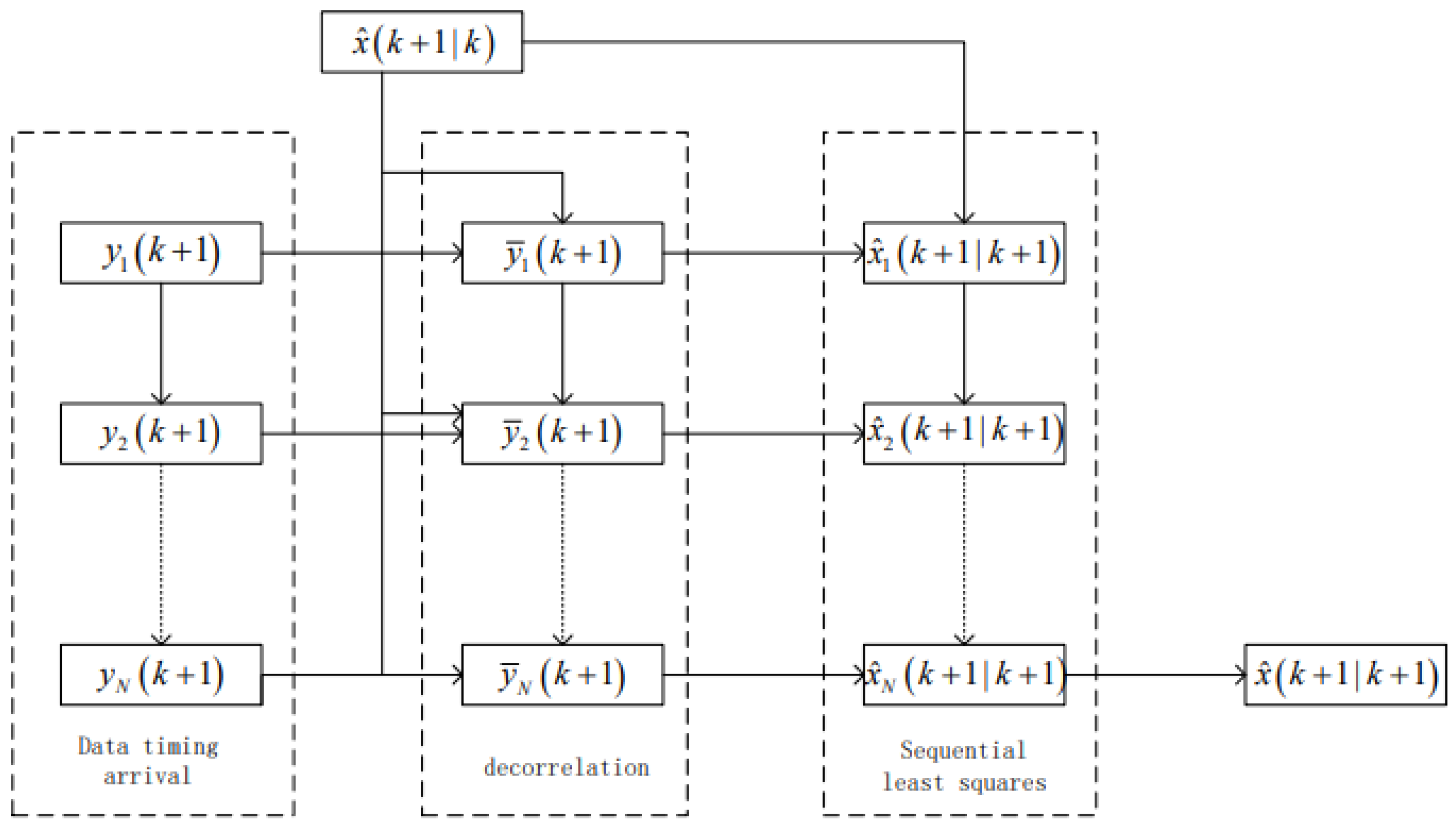
4. A Sequential Least Squares Method for Gradually Decorrelating Time-Series Arrival Data Under Noise Correlation

In this paper, we propose an approach inspired by the Gram–Schmidt orthogonalization method, which integrates stepwise orthogonalization with a sequential fusion least squares algorithm to tackle the multi-sensor fusion filtering problem, where process noise is correlated with measurement noise, and measurement noise exhibits cross-correlation. For generality, we assume that sensor data at the $k+1$-th time step arrive sequentially in the order $y_1,y_2,\dots ,y_N$. The flowchart of the proposed algorithm is presented in Figure 1.

4.1. New Observation Equation for State Based on Predicted Estimates

Based on the state prediction estimation equation, it can also be equivalently expressed as the measurement equation for state $x(k+1)$:

$${\overline{y}}_0\left(k+1\right)={\overline{H}}_0\left(k+1\right)x\left(k+1\right)+{\overline{v}}_0\left(k+1\right)$$

(27)

where ${\overline{y}}_0(k+1)=\widehat{x}(k+1|k)$, ${\overline{H}}_0(k+1)=I$, with $I\in {\mathbb{R}}^{n\times n}$, and ${\overline{v}}_0(k+1)=-\tilde{x}(k+1|k)$.

The random variable ${\overline{v}}_0(k+1)$ satisfies the following statistical properties:

$${\overline{v}}_0(k+1)\sim \mathcal{N}\left(0,{\overline{R}}_0(k+1)\right),{\overline{R}}_0(k+1)=P(k+1|k),$$

Remark 1.

Interpreting (27) as the measurement equation for state variable $x(k+1)$ transforms the challenge of decoupling process noise $v(k+1)$ from measurement noise into a unified decoupling problem involving both measurement noise and the estimation error $\tilde{x}(k+1|k)$. This is because $\tilde{x}(k+1|k)$ is a linear combination of $\tilde{x}\left(k\right|k)$ and $w\left(k\right)$, thereby addressing issues that could not be resolved in the previous literature.

4.2. Estimation Method for State Based on Observation Equation (1)

When data from sensor 1 arrives, the first step is to decorrelate it, since ${\overline{v}}_0\left(k+1\right)$ and $v_1\left(k+1\right)$ are correlated noises; this decorrelation process is analogous to the Schmidt orthogonalization process.

(1) An equivalent reformulation of the observation Equation (1) is

$$\begin{array}{cc}\hfill y_1\left(k+1\right)& =H_1\left(k+1\right)x\left(k+1\right)+v_1\left(k+1\right)+G_1\left(k+1\right)\hfill \\ \hfill & \times \left[{\overline{y}}_0\left(k+1\right)-{\overline{H}}_0\left(k+1\right)x\left(k+1\right)-{\overline{v}}_0\left(k+1\right)\right]\hfill \end{array}$$

(28)

where $G_1\left(k+1\right)$ is the correlation matrix. Combining like terms in the above expression, we obtain

$${\overline{y}}_1\left(k+1\right)={\overline{H}}_1\left(k+1\right)x\left(k+1\right)+{\overline{v}}_1\left(k+1\right)$$

(29)

where

$${\overline{y}}_1(k+1)=y_1(k+1)-G_1(k+1){\overline{y}}_0(k+1)$$

$${\overline{H}}_1(k+1)=H_1(k+1)-G_1(k+1){\overline{H}}_0(k+1)$$

$${\overline{v}}_1(k+1)=v_1(k+1)-G_1(k+1){\overline{v}}_0(k+1)$$

(2) Solve for the correlation matrix $G_1(k+1)$, which is derived from the decorrelation constraint equation $E\left\{{\overline{v}}_1(k+1){\overline{v}}_0{(k+1)}^T\right\}=0$.

$$G_1(k+1)=D_{1,0}(k+1){\overline{R}}_0^{-1}(k+1)$$

$$\begin{array}{cc}\hfill D_{1,0}(k+1)& =E\left\{v_1(k+1)v_0^T(k+1)\right\}\hfill \\ & =-E\left\{v_1(k+1)w{\left(k\right)}^T\right\}\hfill \\ & =-B_1{(k+1)}^T\hfill \end{array}$$

Note: $G_{1,0}(k+1)=G_1(k+1)$.

The augmented measurement noise ${\overline{v}}_1(k+1)$ satisfies the following statistical properties:

$${\overline{v}}_1(k+1)\sim \mathcal{N}\left(0,{\overline{R}}_1(k+1)\right)$$

where

$$\begin{array}{cc}\hfill {\overline{R}}_1(k+1)& =E\left\{{\overline{v}}_1(k+1){\overline{v}}_1^T(k+1)\right\}\hfill \\ & =R_1(k+1)-G_1(k+1)D_{1,0}{(k+1)}^T\hfill \end{array}$$

(3) Establish a least squares estimator based on the state model and the state estimates from sensor 1.

$$\left[\begin{array}{c}{\overline{y}}_0\left(k+1\right)\\ {\overline{y}}_1\left(k+1\right)\end{array}\right]=\left[\begin{array}{c}{\overline{H}}_0\left(k+1\right)\\ {\overline{H}}_1\left(k+1\right)\end{array}\right]x\left(k+1\right)+\left[\begin{array}{c}{\overline{v}}_0\left(k+1\right)\\ {\overline{v}}_1\left(k+1\right)\end{array}\right]$$

(30)

The estimated value is

$$\begin{array}{cc}\hfill {\widehat{\overline{x}}}_1\left(k+1\right)& ={\left[P{\left(k+1|k\right)}^{-1}+{\left(·\right)}_1\right]}^{-1}\hfill \\ \hfill & \times \left[P{\left(k+1|k\right)}^{-1}\widehat{x}\left(k+1|k\right)+{\left(·\right)}_1\right]\hfill \end{array}$$

(31)

where ${\left(·\right)}_i={\overline{H}}_i{\left(k+1\right)}^T{\overline{R}}_i{\left(k+1\right)}^{-1}{\overline{H}}_i\left(k+1\right)$.

Estimation error:

$$\begin{array}{cc}\hfill {\tilde{\overline{x}}}_1\left(k+1\right)& =x\left(k+1\right)-{\widehat{\overline{x}}}_1\left(k+1\right)\hfill \\ \hfill & ={\left[-P{\left(k+1|k\right)}^{-1}-{\left(·\right)}_1\right]}^{-1}\hfill \\ \hfill & \times \left[-P{\left(k+1|k\right)}^{-1}\tilde{x}\left(k+1|k\right)+{\Delta }_1\right]\hfill \end{array}$$

(32)

where ${\Delta }_i={\overline{H}}_i{\left(k+1\right)}^T{\overline{R}}_i{\left(k+1\right)}^{-1}{\overline{v}}_i\left(k+1\right)$.

The state estimation error covariance matrix is

$$\begin{array}{cc}\hfill {\overline{P}}_1\left(k+1\right)& =E\left\{{\tilde{\overline{x}}}_1\left(k+1\right){\tilde{\overline{x}}}_1^T\left(k+1\right)\right\}\hfill \\ \hfill & ={\left[P{\left(k+1|k\right)}^{-1}+{\left(·\right)}_1\right]}^{-1}\hfill \end{array}$$

(33)

4.3. Sequential Least Squares Fusion from Sensor $i\left(i=1,2,\dots ,l-1\right)$ to Sensor l

Assume that the following estimates have been obtained:

$$\begin{array}{c}{\widehat{\overline{x}}}_i\left(k+1\right)\hfill \\ =E\left\{x\left(k+1\right)|{\widehat{x}}_0,y_1\left(k+1\right),\dots ,y_i\left(k+1\right)\right\}\hfill \\ =E\left\{x\left(k+1\right)|{\widehat{x}}_0,{\overline{y}}_1\left(k+1\right),\dots ,{\overline{y}}_i\left(k+1\right)\right\}\hfill \end{array}$$

(34)

The corresponding covariance matrix is given by

$${\overline{P}}_i(k+1)=E\left\{{\tilde{\overline{x}}}_i(k+1){\tilde{\overline{x}}}_i^T(k+1)\right\}$$

(35)

where

$${\tilde{\overline{x}}}_i(k+1)=x(k+1)-{\widehat{\overline{x}}}_i(k+1)$$

The goal of this section is to establish a recursive least squares solution for state $x(k+1)$ after observation $y_l(k+1)$ from sensor l arrives.

$$\begin{array}{c}{\widehat{\overline{x}}}_l\left(k+1\right)\hfill \\ =E\left\{x\left(k+1\right)|{\widehat{x}}_0,y_1\left(k+1\right),\dots ,y_{l-1}\left(k+1\right),y_l\left(k+1\right)\right\}\hfill \\ =E\left\{x\left(k+1\right)|{\widehat{\overline{x}}}_{l-1}\left(k+1\right),{\overline{y}}_l\left(k+1\right)\right\},l=2,3\dots ,N\hfill \end{array}$$

(36)

The corresponding covariance matrix is given by

$${\overline{P}}_l(k+1)=E\left\{{\tilde{\overline{x}}}_l(k+1){\tilde{\overline{x}}}_l^T(k+1)\right\}$$

where

$${\tilde{\overline{x}}}_l(k+1)=x(k+1)-{\widehat{\overline{x}}}_l(k+1)$$

For convenience, we define

$${\overline{Y}}_{l-1}(k+1)={\overline{\phi }}_{l-1}(k+1)x(k+1)+{\overline{V}}_{l-1}(k+1)$$

where

$${\overline{Y}}_{l-1}(k+1)={\left[{\overline{y}}_0^T(k+1),\dots ,{\overline{y}}_{l-1}^T(k+1)\right]}^T$$

$${\overline{V}}_{l-1}(k+1)={\left[{\overline{v}}_0^T(k+1),\dots ,{\overline{v}}_{l-1}^T(k+1)\right]}^T$$

$${\overline{\phi }}_{l-1}(k+1)={\left[{\overline{H}}_0^T(k+1),\dots ,{\overline{H}}_{l-1}^T(k+1)\right]}^T$$

(1) The observation equation for l can be equivalently reformulated as follows:

$$\begin{array}{cc}\hfill y_l(k+1)& =H_l(k+1)x(k+1)+v_l(k+1)+G_l(k+1)\hfill \\ \hfill & \times \left[{\overline{Y}}_{l-1}(k+1)-{\overline{\phi }}_{l-1}(k+1)x(k+1)-{\overline{V}}_{l-1}(k+1)\right]\hfill \end{array}$$

(37)

By combining like terms, we obtain

$${\overline{y}}_l(k+1)={\overline{H}}_l(k+1)x(k+1)+{\overline{v}}_l(k+1)$$

(38)

where

$${\overline{y}}_l(k+1)=y_l(k+1)-G_l(k+1){\overline{Y}}_{l-1}(k+1)$$

$${\overline{H}}_l(k+1)=H_l(k+1)-G_l(k+1){\overline{\phi }}_{l-1}(k+1)$$

$${\overline{v}}_l(k+1)=v_l(k+1)-G_l(k+1){\overline{V}}_{l-1}(k+1)$$

(2) The derivation of the correlation matrix $G_l(k+1)$ is obtained by solving the decorrelation constraint equations $E\left\{{\overline{v}}_l(k+1){\overline{v}}_i{(k+1)}^T\right\}=0$, for $i=1,2,\dots ,l-1$.

$$G_l(k+1)=D_l(k+1){\Lambda }_{l-1}^{-1}(k+1)$$

(39)

where

$$\begin{array}{cc}\hfill D_l(k+1)& =E\left\{v_l(k+1){\overline{V}}_{l-1}{(k+1)}^T\right\}\hfill \\ \hfill & =\left[D_{l,0}(k+1),\dots ,D_{l,l-1}(k+1)\right]\hfill \end{array}$$

(40)

$$\begin{array}{cc}\hfill {\Lambda }_{l-1}(k+1)& =E\left\{{\overline{V}}_{l-1}(k+1){\overline{V}}_{l-1}{(k+1)}^T\right\}\hfill \\ \hfill & =diag\left[{\overline{R}}_0(k+1),\dots ,{\overline{R}}_{l-1}(k+1)\right]\hfill \end{array}$$

(41)

For convenience, we denote

$$G_l(k+1)=\left[G_{l,0}(k+1),\dots ,G_{l,l-1}(k+1)\right]$$

(42)

The statistical properties of ${\overline{v}}_l(k+1)$ are as follows:

$${\overline{v}}_l(k+1)\sim \mathcal{N}\left(0,{\overline{R}}_l(k+1)\right).$$

where

$$\begin{array}{cc}\hfill {\overline{R}}_l(k+1)& =E\left\{{\overline{v}}_l(k+1){\overline{v}}_l{(k+1)}^T\right\}\hfill \\ \hfill & =R_l(k+1)-G_l(k+1)D_l{(k+1)}^T\hfill \end{array}$$

(43)

(3) Develop a sequential least squares fusion estimation framework that incorporates the interactions from sensor i (where $i=1,2,\dots ,l-1$) to sensor l.

The least squares estimator is formulated as follows:

$$\left[\begin{array}{c}{\widehat{\overline{x}}}_{l-1}\left(k+1\right)\\ {\overline{y}}_l\left(k+1\right)\end{array}\right]=\left[\begin{array}{c}I\\ {\overline{H}}_l\left(k+1\right)\end{array}\right]x\left(k+1\right)+\left[\begin{array}{c}-{\tilde{\overline{x}}}_{l-1}\left(k+1\right)\\ {\overline{v}}_l\left(k+1\right)\end{array}\right]$$

(44)

The estimated value is

$$\begin{array}{cc}\hfill {\widehat{\overline{x}}}_l\left(k+1\right)& ={\left[{\overline{P}}_{l-1}^{-1}\left(k+1\right)+{\left(·\right)}_l\right]}^{-1}\hfill \\ \hfill & \times \left[{\overline{P}}_{l-1}^{-1}\left(k+1\right){\widehat{\overline{x}}}_{l-1}\left(k+1\right)+{\left(·\right)}_l\right]\hfill \end{array}$$

(45)

Estimation error:

$$\begin{array}{cc}\hfill {\tilde{\overline{x}}}_l\left(k+1\right)& =x\left(k+1\right)-{\widehat{\overline{x}}}_l\left(k+1\right)\hfill \\ \hfill & ={\left[-{\overline{P}}_{l-1}^{-1}\left(k+1\right)-{\left(·\right)}_l\right]}^{-1}\hfill \\ \hfill & \times \left[-{\overline{P}}_{l-1}^{-1}\left(k+1\right){\tilde{x}}_{l-1}\left(k+1\right)+{\Delta }_l\right]\hfill \end{array}$$

(46)

The state estimation error covariance matrix is

$$\begin{array}{cc}\hfill {\overline{P}}_l\left(k+1\right)& =E\left\{{\tilde{\overline{x}}}_l\left(k+1\right){\tilde{\overline{x}}}_l^T\left(k+1\right)\right\}\hfill \\ \hfill & ={\left[{\overline{P}}_{l-1}^{-1}\left(k+1\right)+{\left(·\right)}_l\right]}^{-1}\hfill \end{array}$$

(47)

When $l=N$, the fusion center can obtain ${\widehat{\overline{x}}}_N\left(k+1\right)$ and ${\overline{P}}_N\left(k+1\right)$, thus establishing the global estimate of $x\left(k+1\right)$ as

$$\begin{array}{c}\hfill {\widehat{\overline{x}}}_N\left(k+1\right)={\left[{\overline{P}}_{N-1}^{-1}\left(k+1\right)+{\overline{H}}_N{\left(k+1\right)}^T{\overline{R}}_N^{-1}\left(k+1\right){\overline{H}}_N\left(k+1\right)\right]}^{-1}\\ \hfill \left[{\overline{P}}_{N-1}^{-1}\left(k+1\right){\widehat{\overline{x}}}_{N-1}\left(k+1\right)+{\overline{H}}_N{\left(k+1\right)}^T{\overline{R}}_N^{-1}\left(k+1\right){\overline{y}}_N\left(k+1\right)\right]\end{array}$$

(48)

$${\overline{P}}_N\left(k+1\right)={\left[{\overline{P}}_{N-1}^{-1}\left(k+1\right)+{\overline{H}}_N{\left(k+1\right)}^T{\overline{R}}_N{\left(k+1\right)}^{-1}{\overline{H}}_N\left(k+1\right)\right]}^{-1}$$

(49)

The sequential least squares estimator is capable of managing systems with observation delays, and the algorithm does not require the acquisition of all data, enabling it to operate effectively even when some data are missing.

To more clearly illustrate the specific implementation steps of the proposed method, the calculation steps of the sequential algorithm are presented below:

Step 1: Establish the initial values $x\left(k|k\right)=x_0$ and $P\left(k|k\right)=P_0$ .

Step 2: Compute $\widehat{x}\left(k+1|k\right)$, $\tilde{x}\left(k+1\left|k\right.\right)$, and $P\left(k+1\left|k\right.\right)$

Step 3: Establish the prediction equation ${\overline{y}}_0\left(k+1\right)={\overline{H}}_0\left(k+1\right)x\left(k+1\right)+{\overline{v}}_0\left(k+1\right)$, where ${\overline{y}}_0\left(k+1\right)=\widehat{x}\left(k+1|k\right)$, ${\overline{H}}_0\left(k+1\right)=I$, and ${\overline{v}}_0\left(k+1\right)=-\tilde{x}\left(k+1|k\right)$

Step 4: Perform decorrelation processing on observation equation $y_1\left(k+1\right)=H_1\left(k+1\right)x\left(k+1\right)+v_1\left(k+1\right)$, resulting in the decorrelated equation ${\overline{y}}_1\left(k+1\right)={\overline{H}}_1\left(k+1\right)$$x\left(k+1\right)+{\overline{v}}_1\left(k+1\right)$

Step 5: Combine the measurement equations from steps 3 and 4 and solve the resulting system using least squares to obtain ${\widehat{\overline{x}}}_1\left(k+1\right)$, ${\tilde{\overline{x}}}_1\left(k+1\right)$, and ${\overline{P}}_1\left(k+1\right)$

Step 6: After fusing data from the current $i=l-1$ sensors, obtain ${\stackrel{\widehat{¯}}{x}}_{l-1}\left(k+1\right)$,${\stackrel{\widetilde{¯}}{x}}_{l-1}\left(k+1\right)$ and ${\overline{P}}_{l-1}\left(k+1\right)$. Perform decorrelation processing on observation equation $y_l\left(k+1\right)=H_l\left(k+1\right)x\left(k+1\right)+v_l\left(k+1\right)$ in the same manner as in step 5.

Step 7: Formulate and solve the system of equations to obtain ${\widehat{\overline{x}}}_l\left(k+1\right)$, ${\tilde{\overline{x}}}_l\left(k+1\right)$, and ${\overline{P}}_l\left(k+1\right)$.

Step 8: If $i=N$, then ${\widehat{\overline{x}}}_N\left(k+1\right)$ and ${\overline{P}}_N\left(k+1\right)$ will be obtained.

5. Performance Equivalence Analysis

This section establishes the equivalence between the proposed sequential least squares recursive algorithm and the centralized Kalman filtering algorithm in the presence of correlated noise. It is shown that their estimation error covariance matrices are identical, indicating equivalent estimation performance. For technical convenience, we define the following notation:

$$\overline{y}(k+1)=\overline{H}(k+1)x(k+1)+\overline{v}(k+1)$$

(50)

where

$${\overline{y}}^T(k+1)=\left[{\overline{y}}_1^T(k+1),\dots ,{\overline{y}}_N^T(k+1)\right]$$

(51)

$$\overline{v}(k+1)={\left[{\overline{v}}_1^T(k+1),\dots ,{\overline{v}}_N^T(k+1)\right]}^T$$

(52)

$$\overline{H}(k+1)={\left[{\overline{H}}_1^T(k+1),\dots ,{\overline{H}}_N^T(k+1)\right]}^T$$

(53)

$$\begin{array}{cc}\hfill \overline{R}(k+1)& =E\left\{\overline{v}(k+1){\overline{v}}^T(k+1)\right\}\hfill \\ \hfill & =\mathrm{diag}\left[{\overline{R}}_1(k+1),\dots ,{\overline{R}}_N(k+1)\right]\hfill \end{array}$$

(54)

Proof of the equivalence between the centralized Kalman filter under correlated noise and the sequential recursive least squares method with stepwise decorrelation is as follows:

First, we can take the centralized measurement noise $\overline{v}\left(k+1\right)$ after decorrelation as an example and establish its relationship with the centralized measurement noise $v\left(k+1\right)$ without decorrelation. Then, we substitute all the parameters of the centralized Kalman filter under correlated noise from Section 3 of this paper with the parameters after decorrelation. The derivation is as follows:

$$\begin{array}{c}\overline{v}\left(k+1\right)={\left[{{\overline{v}}_1}^T\left(k+1\right),{{\overline{v}}_2}^T\left(k+1\right)\dots ,{{\overline{v}}_N}^T\left(k+1\right)\right]}^T\hfill \\ =\left[\begin{array}{c}{v}_1\left(k+1\right)-G_1\left(k+1\right){\overline{v}}_0\left(k+1\right)\\ v_2\left(k+1\right)-G_{2,0}\left(k+1\right){\overline{v}}_0\left(k+1\right)-G_{2,1}\left(k+1\right)v_1\left(k+1\right)\\ ⋮\\ v_N\left(k+1\right)-G_{N,0}\left(k+1\right){\overline{v}}_0\left(k+1\right)-\dots -G_{N,N-1}\left(k+1\right)v_{N-1}\left(k+1\right)\end{array}\right]\hfill \end{array}$$

(55)

Then, $v\left(k+1\right)$ can be expressed as

$$v\left(k+1\right)=M_1\left(k+1\right)\overline{v}\left(k+1\right)+N\left(k+1\right){\overline{v}}_0\left(k+1\right)$$

(56)

where

$$\begin{array}{c}{M}_1\left(k+1\right)=\left[\begin{array}{ccccc}I& 0& 0& \dots & 0\\ G_{2,1}(k+1)& I& 0& \dots & 0\\ G_{3,1}(k+1)& G_{3,2}(k+1)& \ddots & ⋮& ⋮\\ ⋮& ⋮& ⋮& I& 0\\ G_{N,1}(k+1)& G_{N,2}(k+1)& \dots & G_{N,N-1}(k+1)& I\end{array}\right]\hfill \end{array}$$

(57)

$$\begin{array}{c}N\left(k+1\right)=\left[\begin{array}{c}{G}_{1,0}\left(k+1\right)\\ G_{2,0}\left(k+1\right)\\ ⋮\\ G_{N,0}\left(k+1\right)\end{array}\right]\hfill \\ =-S^T\left(k+1\right){\overline{R}}_0{\left(k+1\right)}^{-1}\hfill \end{array}$$

(58)

Likewise, $H\left(k+1\right)$ and $y\left(k+1\right)$ can also be expressed as

$$H\left(k+1\right)=M_1\left(k+1\right)\overline{H}\left(k+1\right)-N\left(k+1\right)H_0{\left(k+1\right)}^{-1}$$

(59)

$$y\left(k+1\right)=M_1\left(k+1\right)\overline{y}\left(k+1\right)+N\left(k+1\right)\widehat{x}\left(k+1|k\right)$$

(60)

In substituting Equations (56), (59), and (60) into Equations (19), (20), (25), and (26), the cross-covariance matrix between the state prediction error and the observation prediction error, the auto-covariance matrix of the observation prediction error, the gain matrix, and the estimation error covariance matrix can be re-expressed as follows:

$$\begin{array}{c}{P}_{\tilde{x}\tilde{y}}\left(k+1|k\right)=E\left\{\tilde{x}\left(k+1|k\right)\tilde{y}{\left(k+1|k\right)}^T\right\}\hfill \\ =P\left(k+1|k\right)\overline{H}{\left(k+1\right)}^T{M}_1{\left(k+1\right)}^T\hfill \end{array}$$

(61)

$$\begin{array}{c}{P}_{\tilde{y}\tilde{y}}\left(k+1|k\right)=E\left\{\tilde{y}\left(k+1|k\right)\tilde{y}{\left(k+1|k\right)}^T\right\}\hfill \\ =M_1\left(k+1\right)\left[\overline{H}\left(k+1\right)P\left(k+1|k\right)\overline{H}{\left(k+1\right)}^T+\overline{R}\left(k+1\right)\right]M_1{\left(k+1\right)}^T\hfill \end{array}$$

(62)

$$\begin{array}{c}K\left(k+1\right)=P_{\tilde{x}\tilde{y}}\left(k+1|k\right)P_{\tilde{y}\tilde{y}}{\left(k+1|k\right)}^{-1}\hfill \\ =P\left(k+1|k\right)\overline{H}{\left(k+1\right)}^T{\left[\overline{H}\left(k+1\right)P\left(k+1|k\right)\overline{H}{\left(k+1\right)}^T+\overline{R}\left(k+1\right)\right]}^{-1}{M}_1{\left(k+1\right)}^{-1}\hfill \end{array}$$

(63)

$$\begin{array}{c}P\left(k+1|k+1\right)=E\left\{\tilde{x}\left(k+1|k+1\right)\tilde{x}{\left(k+1|k+1\right)}^T\right\}\hfill \\ =\left[I-K\left(k+1\right)H\left(k+1\right)\right]P\left(k+1|k\right)-K\left(k+1\right)S{\left(k+1\right)}^T\hfill \\ =\left[I-P\left(k+1|k\right)\overline{H}{\left(k+1\right)}^T{\left(\overline{H}\left(k+1\right)P\left(k+1|k\right)\overline{H}{\left(k+1\right)}^T+\overline{R}\left(k+1\right)\right)}^{-1}\overline{H}\left(k+1\right)\right]P\left(k+1|k\right)\hfill \end{array}$$

(64)

Based on the matrix inversion lemma in reference [28], Equation (64) can be expressed as follows:

$$P\left(k+1|k+1\right)={\left[P^{-1}\left(k+1|k\right)+\overline{H}{\left(k+1\right)}^T\overline{R}{\left(k+1\right)}^{-1}\overline{H}\left(k+1\right)\right]}^{-1}$$

(65)

According to Equation (49), ${\overline{P}}_{N-1}\left(k+1\right)$ can be expressed as

$${\overline{P}}_{N-1}\left(k+1\right)={\left[{\overline{P}}_{N-2}^{-1}\left(k+1\right)+{\overline{H}}_{N-1}{\left(k+1\right)}^T{\overline{R}}_{N-1}{\left(k+1\right)}^{-1}{\overline{H}}_{N-1}\left(k+1\right)\right]}^{-1}$$

(66)

Thus, by analogy, Equation (49) can be expressed as

$$\begin{array}{c}{\overline{P}}_N\left(k+1\right)={\left[{\overline{P}}_{N-1}^{-1}\left(k+1\right)+{\overline{H}}_N{\left(k+1\right)}^T{\overline{R}}_N{\left(k+1\right)}^{-1}{\overline{H}}_N\left(k+1\right)\right]}^{-1}\hfill \\ ={\left[P^{-1}\left(k+1|k\right)+{\displaystyle \sum _{j=1}^N}\left[{\overline{H}}_j^T\left(k+1\right){\overline{R}}_j^{-1}\left(k+1\right){\overline{H}}_j\left(k+1\right)\right]\right]}^{-1}\hfill \end{array}$$

(67)

$P\left(k+1|k+1\right)$ can be expressed as

$$\begin{array}{c}P\left(k+1|k+1\right)={\left[P^{-1}\left(k+1|k\right)+\overline{H}{\left(k+1\right)}^T\overline{R}{\left(k+1\right)}^{-1}\overline{H}\left(k+1\right)\right]}^{-1}\hfill \\ ={\left[P^{-1}\left(k+1|k\right)+{\displaystyle \sum _{j=1}^N}\left[{\overline{H}}_j^T\left(k+1\right){\overline{R}}_j^{-1}\left(k+1\right){\overline{H}}_j\left(k+1\right)\right]\right]}^{-1}\hfill \end{array}$$

(68)

It can be rigorously proved that

$$P(k+1|k+1)\equiv {\overline{P}}_N(k+1)$$

(69)

Therefore, it can be concluded that the sequential least squares algorithm, which relies on the measurement arrival time series ${\overline{y}}_1(k+1),{\overline{y}}_2(k+1),\dots ,{\overline{y}}_N(k+1)$, and the centralized fusion Kalman filtering algorithm, which is based on $y(k+1)$, exhibit identical performance under noise correlation.

6. Simulation Examples

Consider a three-sensor target tracking system with correlated noise:

$$x\left(k+1\right)=\left[\begin{array}{cc}1& T\\ 0& 1\end{array}\right]x\left(k\right)+w\left(k\right)$$

(70)

$$y_i\left(k+1\right)=H_i\left(k+1\right)x\left(k+1\right)+v_i\left(k+1\right)$$

(71)

$$v_i\left(k+1\right)={\alpha }_{i}w\left(k\right)+{\beta }_i\eta \left(k+1\right)$$

(72)

where $i=1,2,3.$ The sampling time is $T=1$. $x\left(k+1\right)=\left[\begin{array}{c}{x}_1\\ x_2\end{array}\right]$ is the state, and $x_1$ and $x_2$ represent the displacement and velocity of the target, respectively. The measurement matrix consists of $H_1\left(k+1\right)=\left[\begin{array}{cc}1& 0\\ 0& 1\end{array}\right]$, $H_2\left(k+1\right)=\left[\begin{array}{cc}1& 0.5\\ 0& 1\end{array}\right]$, and $H_3\left(k+1\right)=\left[\begin{array}{cc}1& 1\\ 0& 1\end{array}\right]$. $w\left(k\right)$ and ${\eta }_i\left(k+1\right)$ are uncorrelated white noise with means of 0 and variances of ${\sigma }_w^2$ and ${\sigma }_{{\eta }_i}^2$, respectively. Let ${\sigma }_w^2=\left[\begin{array}{cc}{\displaystyle \frac{T^3}{3}}& {\displaystyle \frac{T^2}{2}}\\ {\displaystyle \frac{T^2}{2}}& T\end{array}\right]$, ${\sigma }_{{\eta }_1}^2=diag\left[\begin{array}{cc}0.25& 0.25\end{array}\right]$, ${\sigma }_{{\eta }_2}^2=diag\left[\begin{array}{cc}0.36& 0.36\end{array}\right]$, ${\sigma }_{{\eta }_3}^2=diag\left[\begin{array}{cc}0.64& 0.64\end{array}\right]$, ${\beta }_i=1-{\alpha }_i$, ${\alpha }_1=0.1$, ${\alpha }_2=0.2$, ${\alpha }_3=0.4$, ${\beta }_1=0.9$, ${\beta }_2=0.8$, and ${\beta }_3=0.6$. The initial state is $x_0={\left[\begin{array}{cc}2& 2\end{array}\right]}^T$ and $P_0=diag\left[\begin{array}{cc}0.1& 0.1\end{array}\right]$.

The processor sequentially updates the measurements from the three sensors described in (71). For each iteration of the local least squares estimator, the corresponding estimation results and their associated error covariance are computed, thereby demonstrating the equivalence between the proposed algorithm and the centralized algorithm in the simulation. This comparison reveals that both algorithms achieve the same level of estimation accuracy.

The root mean square error (RMSE) is used to evaluate the performance of the algorithm, defined as follows:

$$RMSE=\sqrt{{\displaystyle \frac{1}{N}}\sum _{i=1}^N{\tilde{x}}_i\left(k+1|k+1\right){\tilde{x}}_i{\left(k+1|k+1\right)}^T}$$

(73)

where ${\tilde{x}}_i\left(k+1|k+1\right)=x\left(k+1\right)-{\widehat{x}}_i\left(k+1|k+1\right)$, $\tilde{x}\left(k+1|k+1\right)$ represents the estimation error, $x\left(k+1\right)$ is the true value of the state, $\widehat{x}\left(k+1|k+1\right)$ denotes the estimated state, and N represents the number of simulation runs.

The accuracy is calculated using the mean square error of the first sensor as the reference, as given by the following formula:

$$\epsilon \%={\displaystyle \frac{{\epsilon }_1-{\epsilon }_i}{{\epsilon }_1}}\times 100\%,i=2,3$$

where $\epsilon$ denotes the root mean square error for each sensor.

Remark 2.

“×” shows that this sensor’s RMSE is shown as a reference, and there is no accuracy improvement.

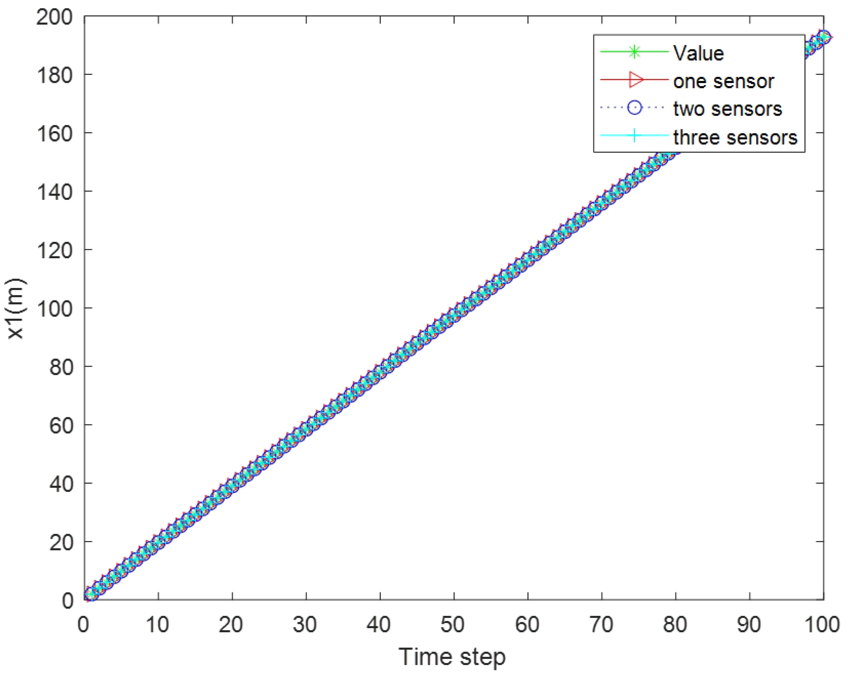
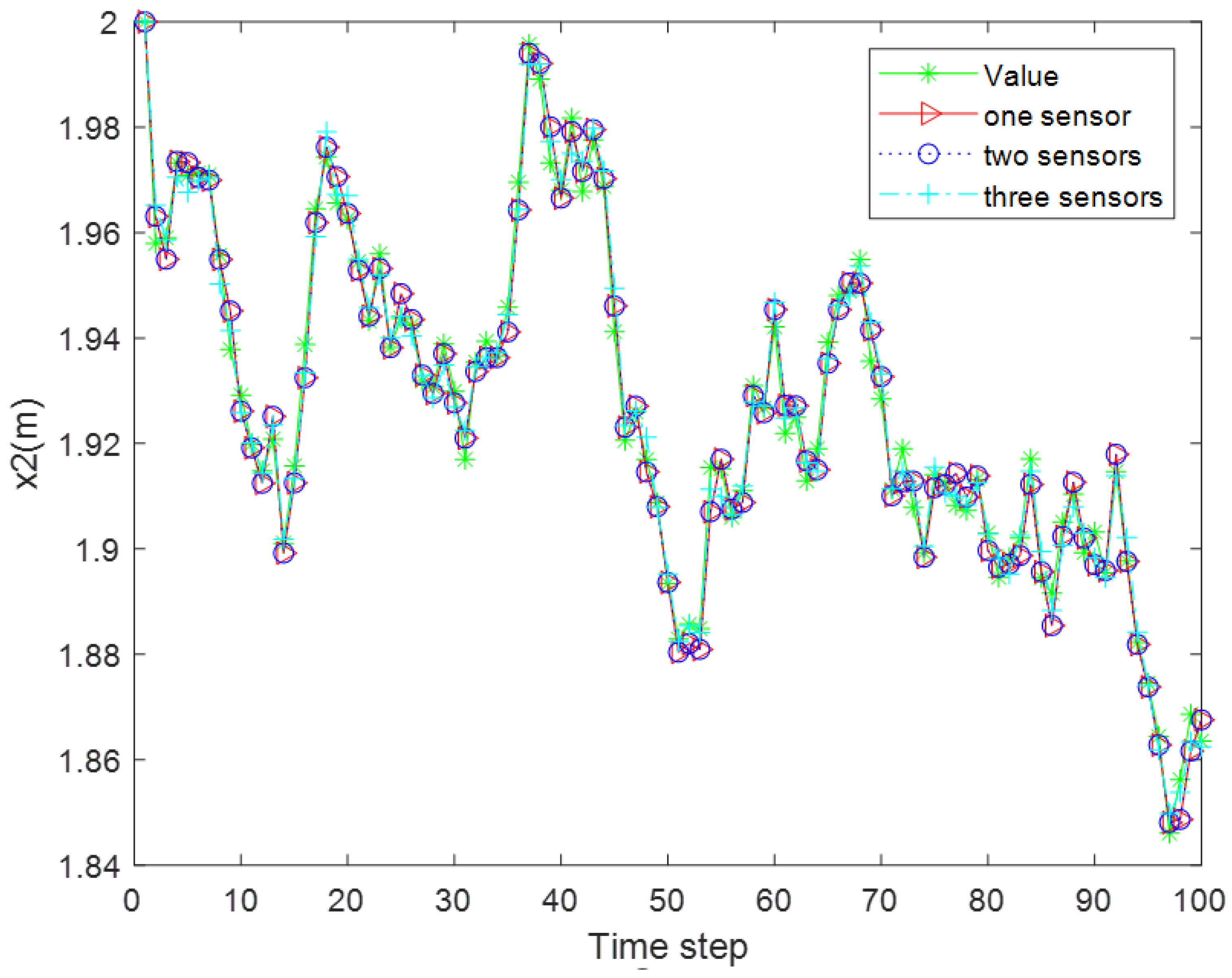
Simulation I : According to the mean square errors shown in

Table 1. Estimation error.

Sensors	RMSE-${\mathit{x}}_1$ (10−3)	RMSE-${\mathit{x}}_2$ (10−3)	Improved-${\mathit{x}}_1$	Improved-${\mathit{x}}_2$
Sensors 1	4.523	4.283	×	×
Sensors 2	3.624	3.432	19.9%	19.9%
Sensors 3	3.149	3.279	30.4%	23.4%

, the accuracy of the estimated state variables has been improved, which demonstrates the effectiveness of the proposed algorithm. Specifically, Figure 2 and Figure 3 show the tracking performance, while Figure 4 and Figure 5 illustrate the estimation error curves.

Simulation II: Figure 6 and Figure 7, respectively, show the comparison of tracking performance between the sequential least squares estimation algorithm proposed in this paper and the centralized fusion Kalman filtering algorithm. The comparison of their estimated results shows that the curves are completely overlapped, indicating that the proposed algorithm has the same estimation accuracy as the centralized fusion algorithm.

Simulation III: The comparison experiment aimed to evaluate the effects of considering versus ignoring noise correlation. We compared the estimation error covariance matrices in both cases. The simulation results show that the algorithm proposed in this paper, which accounts for noise correlation, yields a smaller estimation error covariance matrix, demonstrating superior performance. Furthermore, the comparison of the mean absolute errors is presented as shown in

Table 2. The absolute error means of two algorithms.

Algorithms	MAE-${\mathit{x}}_1$ (10−3)	MAE-${\mathit{x}}_2$ (10−3)
Consider correlation	2.1	1
Ignore correlation	2.4	4.6

.

Simulation IV: To illustrate how the estimation error covariance of the proposed algorithm varies with the correlation coefficient, we kept the correlation coefficients of the first two sensors unchanged and sequentially varied the correlation coefficient of the third sensor.

Table 3. Accuracy of $tr{P}_{-}\left(\alpha \right)$ for $\alpha =-0.6,-0.4,-0.2,0,0.2,0.4,0.6$.

$tr{P}_{-}(-0.6)$	$tr{P}_{-}(-0.4)$	$tr{P}_{-}(-0.2)$	$tr{P}_{-}\left(0\right)$	$tr{P}_{-}\left(0.2\right)$	$tr{P}_{-}\left(0.4\right)$	$tr{P}_{-}\left(0.6\right)$
$0.1182$	$0.1156$	$0.1115$	$0.1046$	$0.0935$	$0.0758$	$0.0499$

presents the trace of the error covariance matrix as the correlation coefficient changes. The relationship of the estimation accuracy can be seen as follows:

$$tr{P}_{-}(-0.6)>tr{P}_{-}(-0.4)>tr{P}_{-}(-0.2)>tr{P}_{-}\left(0\right)>tr{P}_{-}\left(0.2\right)>tr{P}_{-}\left(0.4\right)>tr{P}_{-}\left(0.6\right)$$

Based on the simulation results, it can be seen that as the correlation coefficient increases, the estimation error covariance matrix progressively decreases. This improvement in estimation accuracy further ensures the robustness and effectiveness of the proposed algorithm.

The simulation results demonstrate that the proposed algorithm is capable of effectively addressing multi-sensor systems exhibiting both cross-correlation between process and measurement noise, as well as autocorrelation within the measurement noise. Under noisy conditions, the algorithm attains an accuracy level that matches that of the centralized Kalman filtering algorithm, thereby confirming that the proposed filtering strategy is optimal in the sense of the linear minimum mean square error (LMMSE). Additionally, the algorithm features recursive computation via sequential filtering, ensuring robust performance and practical applicability in real-time scenarios.

7. Conclusions

In the context of discrete-time, time-varying linear stochastic control systems with dual correlations in multi-sensor noise, this paper first treats the state prediction equation as an initial measurement equation. The difficulty of decorrelating process noise from measurement noise is transformed into the problem of jointly decorrelating measurement noise and estimation error. By performing a series of orthogonalizations on the measurement noise subspace of each sensor, the original measurement equation is converted into an equivalent one with uncorrelated noise. Meanwhile, the orthogonalization process preserves the symmetry of the original noise statistics, thereby avoiding additional bias that may arise from asymmetric transformations. Following the principle of sequential filtering, measurement information arriving at the fusion center is processed in sequence. This ensures real-time data fusion and significantly reduces the computational burden associated with high-dimensional matrix operations. The stepwise update adopts a symmetric recursive structure, ensuring both computational efficiency and numerical stability. The resulting estimator achieves global optimality in the sense of linear minimum mean square error (LMMSE) while preserving the statistical symmetry, and the paper provides a rigorous proof of the equivalence between the proposed sequential least squares algorithm, the centralized Kalman filter, and the centralized least-squares algorithm. Simulation results validate the effectiveness of the proposed algorithm.

The proposed method is applicable not only to scenarios with dual correlations—i.e., correlation between process and measurement noise, as well as temporal correlation within the measurement noise—but also to systems with delayed data. However, a limitation of this study is that it does not directly provide a sequential Kalman filter formulation, nor does it address generalized symmetry-preserving methods under correlated noise in nonlinear or non-Gaussian systems. These aspects will be the focus of future work.