Modeling Bimodal and Skewed Data: Asymmetric Double Normal Distribution with Applications in Regression

Abstract

This paper introduces a flexible distribution called the asymmetric double normal distribution, specifically designed to model univariate data exhibiting asymmetry and either unimodal or bimodal characteristics. This distribution is highly flexible, capable of capturing a wide range of data behaviors, from smooth densities to those with thinner tails. It generalizes the skew-normal distribution as a special case and provides a simpler alternative to mixture models by avoiding issues related to parameter identifiability. This study explores the structural and theoretical properties of the asymmetric double normal distribution, and parameter estimation is carried out using the maximum likelihood method. Simulation experiments assess the performance of the estimators, while applications in regression and real-life data fitting illustrate the practical relevance of this model. This proposed distribution proves to be a powerful tool for modeling asymmetric and bimodal data, offering significant advantages for statistical analysis in diverse applications.

1. Introduction

Research on flexible distributions capable of capturing skewness, multimodality, and heavier tails has gained increasing attention in the statistical literature, primarily because traditional normal-based models do not always provide an adequate fit for real-life data. Such endeavors seek to account for diverse distributional shapes, particularly in scenarios with marked skewness or the presence of more than one mode, while maintaining analytical tractability and theoretical coherence. In line with these motivations, the current research proposes the asymmetric double normal (ADN) distribution as a unifying construction to handle asymmetry and potential bimodality in both theoretical investigations and applied statistical modeling.

Before the advent of more comprehensive distributions, the skew-normal model represented one of the main solutions to capture asymmetric data while retaining a normal-like core structure. However, the skew-normal distribution often proved insufficient when the data exhibited more complex patterns, such as heavy tails or multiple modes. Consequently, multiple families of extended normal distributions have been formulated with varying degrees of flexibility. For instance, the two-piece extension of the normal distribution was studied to relax the symmetry constraint by splitting the normal density at a certain threshold and allowing each side to have distinct parameters. These two-piece constructions can be particularly effective for moderate asymmetry but might struggle to capture marked bimodality.

Another prominent line of work involves the introduction of folded- or half-normal transformations. Early foundational work on the folded-normal distribution, such as that by Leone et al. [1], explored its basic properties and estimation techniques. More recently, Tsagris et al. [2] derived characteristic functions, moments, asymptotic inference, and bootstrap confidence intervals for this distribution. These developments underscore the continuing need for adjustments to the classical normal framework in scenarios involving non-negative quantities or pronounced deviations from symmetric behavior. However, folded transformations focus predominantly on data restricted to particular domains (e.g., positive real line), limiting their utility for more general datasets prone to both skewness and potential bimodality.

Bimodality, a critical feature in many real-life datasets (e.g. biomedical markers or athletic performance metrics), has spurred further extensions of the normal paradigm. Salinas et al. [3] proposed the symmetric bimodal two-piece normal (TN) distribution. On a related front, Elal-Olivero et al. [4] developed a family of bimodal skew-normal models, where a skewness parameter allows the model to transition smoothly between unimodal and bimodal shapes. This construction behaves conceptually as a skewed mixture of symmetric distributions. In Bayesian and frequentist contexts, these formulations have demonstrated robust performance in settings where data exhibit significant tail asymmetry or splitting across two separate regions of concentration. Despite these innovations, model complexity and identifiability can impose practical limitations when implementing mixture-like distributions for certain finite-sample applications.

Additional contributions emerge from slash-type distributions, exemplified by the folded-normal slash distribution of Gui et al. [5]. Their model builds upon the absolute value of a normal random variable combined with a power of the uniform distribution to capture heavier-tail behavior in non-negative observations. Although suitable for right-skewed data, slash families do not inherently address bimodality, highlighting the importance of a unifying approach that can simultaneously account for skewness and the possibility of two modes.

Recent explorations into two-piece distributions illuminate an alternative to mixture-based or exponentiated transformations. These approaches focus on a strategic splitting mechanism that allows distinct distributional properties on either side of a cutoff point. Such families, often characterized by a shape parameter that governs transitions between unimodality and bimodality, can even revert to the normal distribution in special cases. Notably, these constructions demonstrate how a parameter controlling curvature or skewness can introduce multimodal phenomena without invoking discrete mixing. Because two-piece structures often remain analytically tractable, especially with regard to cumulative distribution functions, likelihood-based parameter estimation, and regression, these methods suggest a template for more general double-asymmetric formulations.

The ADN framework adapts the foundational insights from two-piece modeling and skew-elliptical approaches, but expands the flexibility to accommodate pronounced asymmetry on both tails, along with the potential for bimodality. The need for such flexible models is evident in various fields; for instance, in economics, income distributions often exhibit significant skewness and can occasionally present bimodality reflecting different population subgroups [6], while in biostatistics, the distribution of certain biomarkers or physiological measurements can be asymmetrically distributed and present multiple modes indicative of different health statuses or responses to treatment [7]. The development of the ADN distribution responds to limitations identified in previous skew-normal or mixture-based families when faced with such complex data structures, while ensuring that methods such as maximum likelihood maintain validity in finite and large-sample conditions. Moreover, because earlier work emphasizes that different distributions can be nested or specialized cases of broader families (Elal-Olivero et al. [4]; Bolfarine et al. [8]), the ADN distribution is conceived to encompass normal and skew-normal forms as boundary or limiting instances.

The central objective of this research is to formalize the ADN distribution, defining its probability density function (PDF), the cumulative distribution function (CDF), and its principal theoretical properties. This work addresses the need for univariate models capable of flexibly and parsimoniously capturing both asymmetry and potential bimodality, characteristics frequently observed in real-world datasets where standard normal or skew-normal distributions may prove insufficient, and simpler alternatives to complex mixture models are desired. By incorporating dual-shape parameters, the ADN distribution aims to capture left- and right-sided asymmetry and, depending on their interplay, produce unimodal or bimodal contours. Such a dual-purpose construction provides a natural and analytically tractable alternative to existing skewed models or mixtures of distributions to handle data with these complex features.

In previous studies involving real-life datasets, it was emphasized that skew families and two-piece distributions can perform exceptionally well out of sample, especially when data deviate from normality (Bolfarine et al. [8]; Arnold et al. [9]). The study aims to further evaluate the ADN distribution within medical and sports datasets, particularly focusing on those with bimodal or highly skewed distributions. Through these assessments, we demonstrate not just the practical adaptability of the ADN distribution but also its ability to maintain a streamlined parameterization compared to traditional mixture models.

Moreover, this research seeks to extend the application of the ADN distribution to regression scenarios, where the assumption of normal error terms often falls short. By integrating ADN errors into linear or generalized linear models, we aim to provide a more accurate depiction of real-life phenomena characterized by elongated tails, asymmetric behavior, or bimodal patterns within residual distributions. By utilizing inference methods similar to those developed for classical normal theory, but modified to include shape parameters, ADN has the potential to broaden the horizons of parametric regression modeling.

Before introducing the stochastic representation of the new ADN variable, we first define some well-known distributions in the existing literature.

Definition 1.

The skew-normal distribution (Azzalini [10]) is a natural extension of the normal distribution, introducing a skewness parameter $\alpha \in \mathbb{R}$ that allows for modeling asymmetric data. The PDF of a random variable X, denoted as $X\sim SN\left(\alpha \right)$, is given by

$${\varphi }_{\alpha }\left(x\right)=2\varphi \left(x\right)\mathsf{\Phi }\left(\alpha x\right),x,\alpha \in \mathbb{R},$$

(1)

where ϕ and Φ are the PDF and CDF of $N(0,1)$ (the standard normal distribution), respectively.

The folded-normal distribution (FN), originally proposed by Leone et al. [1], extends the normal distribution by taking the absolute value of the standard normal random variable. It is defined by its location and scale parameters and has been widely studied for its references in asymmetric data modeling. This distribution is widely recognized for its utility in modeling asymmetric data, particularly in applications where only the magnitude of the data is of interest, such as reliability studies, survival analysis, and signal processing. Its moments, skewness, and kurtosis have been extensively studied, providing a foundation for both theoretical and applied work.

Definition 2.

The folded-normal distribution with parameters $(\mu ,\sigma )$ defines the distribution of the random variable $Y=\left|U\right|$, where U is normally distributed with mean μ and variance ${\sigma }^2$. The PDF of Y is

$$f_Y(y;\mu ,\sigma )={\displaystyle \frac{1}{\sigma }}\sqrt{{\displaystyle \frac{2}{\pi }}}{e}^{-(y^2+{\mu }^2)/2{\sigma }^2}\cosh \left({\displaystyle \frac{\mu }{{\sigma }^2}}y\right),y>0.$$

Using a convenient reparameterization $(\mu ,\sigma )$ by $(\lambda ,\sigma )$, where $\lambda =\mu /\sigma$, the PDF can be expressed as another version, denoted $FN(\lambda ,\sigma )$; then,

$$f_Y(y;\lambda ,\sigma )={\displaystyle \frac{2}{\sigma }}\varphi \left({\displaystyle \frac{y}{\sigma }}\right)e^{-{\lambda }^2/2}\cosh \left(\lambda {\displaystyle \frac{y}{\sigma }}\right),y>0,$$

(2)

where ϕ is the PDF of the standard normal distribution.

Remark 1.

Let $Y\sim FN(\lambda ,1)$; the PDF can be expressed as

$$f_Y(y;\lambda )=\varphi (y-\lambda )+\varphi (y+\lambda ),y,\lambda \ge 0.$$

(3)

2. The Family of Uni/Bimodal Densities

In this section, we introduce a new class of distributions, termed the asymmetric double normal distribution, designed to model data with varying degrees of asymmetry, and this takes us to bimodality as another feature. This flexible distributional family provides a valuable alternative to existing asymmetric bimodal distributions in the literature. We also explore the unimodality and bimodality properties of this distribution, presenting key results and insights to analyze the variability of different data types in unimodal and bimodal scenarios, thus capturing diverse patterns commonly observed in real-life datasets.

Definition 3.

It is said that the random variable has an asymmetric double normal distribution with parameters α and λ, denoted by $Z\sim ADN(\lambda ,\alpha )$, if its PDF is given by

$$f_Z(z;\lambda ,\alpha )={\varphi }_{\alpha }\left(z\right)e^{-{\lambda }^2/2}\cosh \left(\lambda z\right),z\in \mathbb{R},\alpha \in \mathbb{R},\lambda \ge 0,$$

(4)

where ${\varphi }_{\alpha }$ is given in Equation (1).

The ADN distribution generalizes the skew-normal and two-piece normal distributions, combining parameters ($\lambda$ for shape, $\alpha$ for skewness) to capture both unimodal and bimodal behaviors. Hence, the ADN provides a uniform framework for switching between symmetric, skewed, and bimodal scenarios by including the normal, skew-normal, and folded normal distributions as special cases. Its versatility enables it to simulate real-life data with bimodality, thinner tails, or asymmetry, all of which are prevalent in domains such as biology, environmental science, and finance. In contrast to finite mixture models (such as two-component normals), the ADN achieves bimodality and captures complex shapes through a single unified distributional structure rather than by mixing separate components. This approach can simplify the modeling process and mitigate some of the computational complexities often associated with fitting mixture models. The ADN restores the mathematical properties of the normal distribution (such as closed-form formulas for moments, CDF, and MGF) while incorporating asymmetry. Simple simulation and parameter estimation with maximum likelihood techniques are made possible by its stochastic representation (via folded-normal and Bernoulli variables).

Figure 1 illustrates density plots of the ADN distribution for different values of parameters $\lambda$ and $\alpha$. The densities can exhibit either unimodal or bimodal behavior depending on the parameter values. In particular, the densities are plotted for $\alpha >0$; When $\alpha$ takes negative values, the resulting density is a reflection with respect to the origin of the density corresponding to positive values. The plots in this figure illustrate how skewness and kurtosis change depending on these parameter values.

The ADN distribution can be viewed as a weighted version of the skew-normal distribution ${\varphi }_{\alpha }\left(z\right)$ with the weight function $\cosh \left(\lambda z\right)$, that is, $f_Z(z;\lambda ,\alpha )={\displaystyle \frac{\cosh \left(\lambda z\right){\varphi }_{\alpha }\left(z\right)}{\mathbb{E}\left(\cosh \right(\lambda Z)}}$, where the normalization constant $\mathbb{E}\left(\cosh \left(\lambda Z\right)\right)=e^{{\lambda }^2/2}$ (see Appendix A).

Remark 2.

The PDF (4) can be represented as a sum of two functions, i.e.,

$$f_Z(z;\lambda ,\alpha )=(\varphi (z-\lambda )+\varphi (z+\lambda ))\mathsf{\Phi }\left(\alpha z\right).$$

(5)

We refer to this distribution as the asymmetric double normal distribution. This name highlights the combination of two normal densities ($\varphi (z-\lambda )+\varphi (z+\lambda )$) and the asymmetry introduced by the skew mechanism $\mathsf{\Phi }\left(\alpha z\right)$. This distribution belongs to a general class of asymmetric distributions. It is a way of modulating a symmetric density by a cumulative distribution function. Here, the base density is $f_0\left(z\right)=(\varphi (z-\lambda )+\varphi (z+\lambda ))/2$, which is the PDF of an equal mixture of two normal distributions $N(\lambda ,1)$ and $N(-\lambda ,1)$. This density $f_0\left(z\right)$ has about zero symmetry. The function that introduces the asymmetry is $2\mathsf{\Phi }\left(\alpha z\right)$.

Furthermore, various properties can be derived from the definition of the asymmetric double normal distribution. The fundamental characteristics of the class $ADN(\alpha ,\lambda )$ can be obtained directly from Equation (4).

Proposition 1.

If $Z\sim ADN(\lambda ,\alpha )$, then the CDF is given by

$$F(z;\lambda ,\alpha )=G(z-\lambda ,\alpha z)+G(z+\lambda ,\alpha z),$$

where

$$G(x,y)={\int }_{-\infty }^x{\int }_{-\infty }^y\varphi \left(u\right)\varphi \left(v\right)dudv.$$

Proof. 

From the definition of the CDF and using Equation (5), we get

$$\begin{array}{ccc}\hfill P(Z\le z)& =& {\int }_{-\infty }^z\varphi (x-\lambda )\mathsf{\Phi }\left(\alpha x\right)dx+{\int }_{-\infty }^z\varphi (x+\lambda )\mathsf{\Phi }\left(\alpha x\right)dx\hfill \\ & =& {\int }_{-\infty }^{z-\lambda }\varphi \left(u\right)\mathsf{\Phi }\left(\alpha (u+\lambda )\right)du+{\int }_{-\infty }^{z+\lambda }\varphi \left(u\right)\mathsf{\Phi }\left(\alpha (u-\lambda )\right)du\hfill \\ & =& {\int }_{-\infty }^{z-\lambda }{\int }_{-\infty }^{\alpha (u+\lambda )}\varphi \left(u\right)\varphi \left(v\right)dvdu+{\int }_{-\infty }^{z+\lambda }{\int }_{-\infty }^{\alpha (u-\lambda )}\varphi \left(u\right)\varphi \left(v\right)dvdu.\hfill \end{array}$$

Now, when we evaluate the limits of integration, we observe the following: For the first integral, when $u=z-\lambda$ (the upper limit), $u+\lambda =z$. Thus, $\alpha (u+\lambda )=\alpha z$. For the second integral, when $u=z+\lambda$ (the upper limit), $u-\lambda =z$. Thus, $\alpha (u-\lambda )=\alpha z$.

Therefore, using the definition of $G(x,y)$, we have

$$\begin{array}{ccc}\hfill P(Z\le z)& =& G(z-\lambda ,\alpha z)+G(z+\lambda ,\alpha z),\hfill \end{array}$$

which gives the desired outcome.    □

This result provides an explicit and interpretable representation of the CDF for the asymmetric double normal distribution, expressed in terms of the integrals of standard normal densities. This formulation not only highlights the role of the shape parameters ($\lambda$) and skewness ($\alpha$) but also facilitates practical applications, including numerical evaluation and simulation.

Remark 3.

The $ADN(\lambda ,\alpha )$ distribution lacks a closed-form expression for its quantile function due to the complexity of the CDF, which involves bivariate integrals of the standard normal density. Finding the p-th quantile $q_p$ requires solving

$$F(q_p;\lambda ,\alpha )=G(q_p-\lambda ,\alpha q_p)+G(q_p+\lambda ,\alpha q_p)=p.$$

This equation is not analytically solvable due to the non-linear dependence of $q_p$ within the function G. For practical applications, we recommend numerical approaches: root-finding methods (Newton–Raphson, bisection), interpolation using precomputed CDF values, or Monte Carlo simulations for less precision-critical applications. For implementation, we suggest combining bisection with Newton–Raphson iterations. The absence of closed-form quantiles is common in complex distributions and does not diminish the practical utility of the $ADN(\lambda ,\alpha )$ distribution.

3. Some Properties of the ADN Distribution

In this section, we explore the statistical properties of the ADN distribution, focusing on its fundamental characteristics, stochastic representation, and moment-generating function.

3.1. Basic Properties

The following properties can be obtained directly from Definition 3.

Properties 1.

Let $Z\sim ADN(\lambda ,\alpha )$; the following properties hold:

(a) 

$f_Z(z;\lambda =0,\alpha =0)=\varphi \left(z\right)$.

(b) 

$f_Z(z;\lambda =0,\alpha )={\varphi }_{\alpha }\left(z\right)$.

(c) 

$f_Z(z;\lambda ,\alpha =0)=\varphi \left(z\right)e^{-{\lambda }^2/2}\cosh \left(\lambda z\right)$.

(d) 

$\left|Z\right|\stackrel{d}{=}\left|X\right|\sim FN(\lambda ,1)$, where $X\sim N(\lambda ,1)$.

(e) 

$-Z\sim {\varphi }_{\alpha }(-z)e^{-{\lambda }^2/2}\cosh \left(\lambda z\right)$.

(f) 

$\underset{\lambda \to 0}{lim}{f}_Z(z;\lambda ,\alpha )={\varphi }_{\alpha }\left(z\right)$. In contrast, as $\lambda \to \infty$, $f_Z(z;\lambda ,\alpha )$ tends to degenerate at 0.

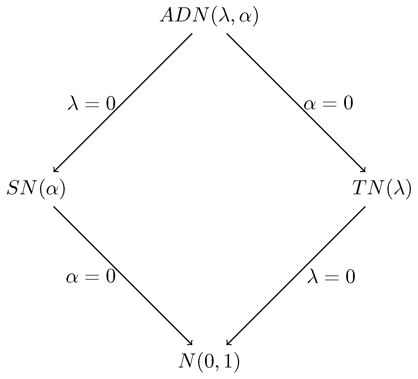
Property (a) shows that the ADN distribution includes the normal distribution as a special case when $\lambda =0$ and $\alpha =0$, and it has similar properties to the normal distribution that make it a useful and applicable distribution in real-life applications. Property (b) establishes that for $\lambda =0$ and any $\alpha$, the ADN density becomes an even function, ${\varphi }_{\alpha }\left(z\right)$, making it asymmetric around the y-axis. Property (c) shows that when the skewness parameter is $\alpha =0$, the ADN density is reduced to $\varphi \left(z\right)e^{-{\lambda }^2/2}\cosh \left(\lambda z\right)$. This specific form is recognized in the literature as the two-piece normal distribution, denoted $TN\left(\lambda \right)$. Property (d) shows that the distribution of the absolute value of Z follows the folded-normal distribution, $FN(\lambda ,1)$, which is the distribution of $\left|X\right|$ when $X\sim N(\lambda ,1)$. Property (e) illustrates the asymmetry of the ADN density around zero. Property (f) indicates that as $\lambda \to 0$, $f_Z(z;\lambda ,\alpha )$ approaches ${\varphi }_{\alpha }\left(z\right)$, the ADN density simplifies to a symmetric form.

On the other hand, as $\lambda \to \infty$, $f_Z(z;\lambda ,\alpha )$ becomes concentrated at zero, this leads to a degenerate distribution. These properties provide insights into the behavior and flexibility of the ADN distribution, highlighting its ability to exhibit symmetry, asymmetry, and degeneracy for different parameter configurations. This flexibility will be used in subsequent sections for statistical inference and applications.

Remark 4.

The PDF given in Equation (4) exhibits interesting properties due to its composition of normal density $\varphi \left(x\right)$, normal CDF $\mathsf{\Phi }\left(\alpha x\right)$, and hyperbolic cosine term $\cosh \left(\lambda x\right)$. The derivative

$${\displaystyle \frac{d{f}_Z(z;\lambda ,\alpha )}{dz}}=-z+{\displaystyle \frac{\alpha \varphi \left(\alpha z\right)}{\mathsf{\Phi }\left(\alpha z\right)}}+\lambda tanh\left(\lambda z\right)$$

reveals that the critical points and thus the maxima depend on a balance between the linear term $-z$, the ratio involving $\varphi \left(\alpha z\right)/\mathsf{\Phi }\left(\alpha z\right)$, and the non-linear term $\lambda tanh\left(\lambda z\right)$. This structure suggests that the density is asymmetric and multimodal, with the number and location of the modes being heavily influenced by the parameters α and λ. Numerical methods are essential for locating these modes, as the derivative equation lacks a closed-form solution. This density is particularly suited for modeling skewed and heavy-tailed distributions in various applications.

Figure 2 illustrates the submodels of the ADN distribution depending on the values of the parameters $\lambda$ and $\alpha$. Specifically, when $\lambda =0$ and $\alpha =0$, the ADN distribution simplifies to the standard normal distribution $N(0,1)$, while for $\lambda =0$ and $\alpha \ne 0$, it becomes the skew-normal distribution $SN\left(\alpha \right)$, showing asymmetry. When $\alpha =0$ and $\lambda \ne 0$, the ADN distribution becomes $TN\left(\lambda \right)$. Moreover, the absolute value of Z, denoted $\left|Z\right|$, follows a folded-normal distribution $FN(\lambda ,1)$, reflecting the behavior of $\left|X\right|$ when $X\sim N(\lambda ,1)$. These special cases highlight the flexibility of the ADN distribution, allowing it to model symmetric and skewed behaviors.

3.2. Stochastic Representation of the ADN Random Variable

The following proposition presents the mechanism for generating random numbers that follow the ADN distribution.

Proposition 2.

$Z\sim ADN(\alpha ,\lambda )$ if and only if there exist dependent random variables S and $Y\sim FN(\lambda ,1)$ with $P(S=1|Y=y)=1-P(S=-1|Y=y)=\mathsf{\Phi }\left(\alpha y\right)$, such that $Z\stackrel{d}{=}SY$.

Proof. 

Let S and Y be defined as in the statement of the proposition. Using the joint distribution of $(Z,S)$ and the Jacobian method, the marginal distribution of Z is obtained as follows: If $Z\ge 0$, then $Z=Y$ and $S=1$. Therefore, we have

$$\begin{array}{ccc}\hfill f_Z(z;\alpha ,\lambda )& =& f_Y\left(z\right)P(S=1|Y=z)\hfill \\ & =& 2\varphi \left(z\right)e^{-{\lambda }^2/2}\cosh \left(\lambda z\right)\mathsf{\Phi }\left(\alpha z\right)\hfill \\ & =& {\varphi }_{\alpha }\left(z\right)e^{-{\lambda }^2/2}\cosh \left(\lambda z\right).\hfill \end{array}$$

On the other hand, if $Z<0$, then $Z=-Y$ and $S=-1$, as follows:

$$\begin{array}{ccc}\hfill f_Z(z;\alpha ,\lambda )& =& f_Y(-z)P(S=-1|Y=-z)\hfill \\ & =& 2\varphi (-z)e^{-{\lambda }^2/2}\cosh (-\lambda z)(1-\mathsf{\Phi }(-\alpha z))\hfill \\ & =& 2\varphi \left(z\right)e^{-{\lambda }^2/2}\cosh \left(\lambda z\right)\mathsf{\Phi }\left(\alpha z\right)\hfill \\ & =& {\varphi }_{\alpha }\left(z\right)e^{-{\lambda }^2/2}\cosh \left(\lambda z\right).\hfill \end{array}$$

   □

This stochastic representation of the random variable $Z\sim ADN(\alpha ,\lambda )$ highlights its structure as a combination of two components: a random sign, represented by S, and a non-negative magnitude modeled by the folded-normal distribution $Y\sim FN(\lambda ,1)$. This construction not only provides an intuitive understanding of Z but also underscores the flexibility of the ADN distribution to represent patterns of asymmetry and bimodality observed in real-life data. By combining the inherent asymmetry of the folded-normal distribution with the additional control introduced by the parameter $\alpha$, this distribution becomes a valuable tool to model phenomena that exhibit opposing directions or contrasting behaviors, such as those encountered in financial studies, biostatistics, and directional data analysis. Moreover, the stochastic representation facilitates simulations and numerical computations, enhancing its applicability in both practical and methodological analyses.

3.3. Derivation of Moments for the ADN Distribution

The random variable Z can be represented as a combination of two dependent random variables S and Y, as shown in Proposition 2. In this section, we derive a formula for computing the r-th moment of a random variable X that follows the $ADN\left(\theta \right)$ distribution, where $\theta ={(\xi ,\eta ,\lambda ,\alpha )}^{\prime }$ and $X=\xi +\eta Z$, with $Z\sim ADN(\lambda ,\alpha )$.

Proposition 3.

Let $Y\sim FN(\lambda ,1)$; the r-th moment of Y is given by

$$\mathbb{E}\left(Y^k\right)=\sum _{j=0}^k\left({\displaystyle \genfrac{}{}{0pt}{}{k}{j}}\right){\lambda }^{k-j}\left[I_j(-\lambda )+{(-1)}^{k-j}{I}_j\left(\lambda \right)\right],$$

where $I_j\left(a\right)={\int }_a^{\infty }{u}^j\varphi \left(u\right)du$ is the incomplete normal moments.

Proof. 

Using Equation (3) and the definition of moments, we have

$$\begin{array}{ccc}\hfill \mathbb{E}\left(Y^k\right)& =& {\int }_0^{\infty }{y}^k[\varphi (y-\lambda )+\varphi (y+\lambda )]dy\hfill \\ & =& {\int }_0^{\infty }{y}^k\varphi (y-\lambda )dy+{\int }_0^{\infty }{y}^k\varphi (y+\lambda )dy\hfill \\ & =& {\int }_{-\lambda }^{\infty }{(u+\lambda )}^k\varphi \left(u\right)du+{\int }_{\lambda }^{\infty }{(u-\lambda )}^k\varphi \left(u\right)du\hfill \\ & =& {\int }_{-\lambda }^{\infty }\sum _{j=0}^k\left({\displaystyle \genfrac{}{}{0pt}{}{k}{j}}\right)u^j{\lambda }^{k-j}\varphi \left(u\right)du+{\int }_{\lambda }^{\infty }\sum _{j=0}^k\left({\displaystyle \genfrac{}{}{0pt}{}{k}{j}}\right)u^j{(-\lambda )}^{k-j}\varphi \left(u\right)du\hfill \\ & =& \sum _{j=0}^k\left({\displaystyle \genfrac{}{}{0pt}{}{k}{j}}\right){\lambda }^{k-j}\left[{\int }_{-\lambda }^{\infty }{u}^j\varphi \left(u\right)du+{(-1)}^{k-j}{\int }_{\lambda }^{\infty }{u}^j\varphi \left(u\right)du\right]\hfill \\ & =& \sum _{j=0}^k\left({\displaystyle \genfrac{}{}{0pt}{}{k}{j}}\right){\lambda }^{k-j}\left[I_j(-\lambda )+{(-1)}^{k-j}{I}_j\left(\lambda \right)\right].\hfill \end{array}$$

   □

Proposition 4.

Using Lin’s [11] results, we have

$$I_j\left(\lambda \right)=\left\{\begin{array}{cc}1-\mathsf{\Phi }\left(\lambda \right),& j=0,\\ (j-1)I_{j-2}\left(\lambda \right)+{\lambda }^{j-1}\varphi \left(\lambda \right),& j=1,2,3,\dots \end{array}\right.$$

(6)

where $\lambda >0$.

Proof. 

For $j=0$, we have $I_0\left(\lambda \right)={\int }_{\lambda }^{\infty }\varphi \left(u\right)du=1-\mathsf{\Phi }\left(\lambda \right)$. For $j=1,2,3,\dots$, we will derive the expression $u^{j-1}\varphi \left(u\right)$, as follows:

$$\begin{array}{ccc}\hfill d\left(u^{j-1}\varphi \left(u\right)\right)& =& (j-1)u^{j-2}\varphi \left(u\right)du+u^{j-1}(-u\varphi \left(u\right))du\hfill \\ & =& (j-1)u^{j-2}\varphi \left(u\right)du-u^j\varphi \left(u\right)du\hfill \\ \hfill u^j\varphi \left(u\right)du& =& (j-1)u^{j-2}\varphi \left(u\right)du-d\left(u^{j-1}\varphi \left(u\right)\right)\hfill \\ \hfill {\int }_{\lambda }^{\infty }{u}^j\varphi \left(u\right)du& =& (j-1){\int }_{\lambda }^{\infty }{u}^{j-2}\varphi \left(u\right)du-{\int }_{\lambda }^{\infty }d\left(u^{j-1}\varphi \left(u\right)\right)\hfill \\ \hfill I_j\left(\lambda \right)& =& (j-1)I_{j-2}\left(\lambda \right)+{\lambda }^{j-1}\varphi \left(\lambda \right).\hfill \end{array}$$

   □

Corollary 1.

$$I_j(-\lambda )=\left\{\begin{array}{cc}\mathsf{\Phi }\left(\lambda \right),& j=0,\\ (j-1)I_{j-2}(-\lambda )+{(-\lambda )}^{j-1}\varphi \left(\lambda \right),& j=1,2,3,\dots \end{array}\right.$$

(7)

where $\lambda >0$.

Proposition 5.

Let $Y\sim FN(\lambda ,1)$; then,

$$\begin{array}{ccc}\hfill \mathbb{E}\left(Y\right)& =& 2\left(\lambda \mathsf{\Phi }\right(\lambda )+\varphi (\lambda \left)\right)-\lambda \hfill \\ \hfill Var\left(Y\right)& =& {\lambda }^2+1\hfill \end{array}$$

Proof. 

Using Proposition 4 and Corollary 1, it follows that

$$\begin{array}{ccc}\hfill I_0\left(\lambda \right)& =& 1-\mathsf{\Phi }\left(\lambda \right)\hfill \\ \hfill I_0(-\lambda )& =& \mathsf{\Phi }\left(\lambda \right)\hfill \\ \hfill I_1\left(\lambda \right)& =& I_1(-\lambda )=\varphi \left(\lambda \right)\hfill \\ \hfill I_2\left(\lambda \right)& =& I_0\left(\lambda \right)+\lambda \varphi \left(\lambda \right)=1-\mathsf{\Phi }\left(\lambda \right)+\lambda \varphi \left(\lambda \right)\hfill \\ \hfill I_1(-\lambda )& =& I_0(-\lambda )-\lambda \varphi \left(\lambda \right)=\mathsf{\Phi }\left(\lambda \right)-\lambda \varphi \left(\lambda \right)\hfill \end{array}$$

Then, applying Proposition 3, we have the results.    □

Proposition 6.

Let $X\sim ADN\left(\theta \right)$; the r-th moment of X is given by

$$\mathbb{E}\left(X^r\right)=\sum _{k=0}^r\left({\displaystyle \genfrac{}{}{0pt}{}{r}{k}}\right){\xi }^{r-k}{\eta }^k\mathbb{E}\left(Z^k\right),$$

(8)

where $\mathbb{E}\left(Z^k\right)$ is given by

$$\mathbb{E}\left(Z^k\right)=\left\{\begin{array}{cc}\mathbb{E}\left(Y^k\right),\hfill & \mathit{if}k\mathit{is}\mathit{even},\hfill \\ 2\mathbb{E}\left(Y^k\mathsf{\Phi }\left(\lambda Y^2\right)\right)-\mathbb{E}\left(Y^k\right),\hfill & \mathit{if}k\mathit{is}\mathit{odd},\hfill \end{array}\right.$$

(9)

and $Y\sim FN(\lambda ,1)$ is the random variable in the stochastic representation of Z, as given in Proposition 2.

Proof. 

Applying the stochastic representation provided in Proposition 2 and applying the properties of conditional expectation, we can derive the required expression as follows.

$$\begin{array}{ccc}\hfill \mathbb{E}\left(Z^k\right)& =& \mathbb{E}\left(\mathbb{E}\left(Z^k\right|Y)\right)\hfill \\ & =& \mathbb{E}(Y^k\mathsf{\Phi }\left(\alpha Y\right)+{(-1)}^k{Y}^k(1-\mathsf{\Phi }\left(\alpha Y\right)))\hfill \\ & =& \mathbb{E}((1-{(-1)}^k)Y^k\mathsf{\Phi }\left(\alpha Y\right)+{(-1)}^k{Y}^k).\hfill \end{array}$$

The above leads to the conclusion that if k is even, then $\mathbb{E}\left(Z^k\right)=\mathbb{E}\left(Y^k\right)$. On the other hand, if k is odd, then $\mathbb{E}\left(Z^k\right)=2\mathbb{E}\left(Y^k\mathsf{\Phi }\left(\alpha Y\right)\right)-\mathbb{E}\left(Y^k\right)$. To obtain $\mathbb{E}\left(X^k\right)$, it is possible to apply the binomial theorem along with the basic properties of the expectation.    □

The mean and variance of a random variable X with the ADN distribution can be easily calculated using the following corollary.

Corollary 2.

Let $Z\sim ADN(\lambda ,\alpha )$ and $X=\xi +\eta Z\sim ADN\left(\theta \right)$. Then, the mean and variance of X are given by

$$\mathbb{E}\left(X\right)=\xi +\eta (2b_1-a_1)andVar\left(X\right)={\eta }^2(a_2-{(2b_1-a_1)}^2),$$

(10)

where $a_1=2(\lambda \mathsf{\Phi }\left(\lambda \right)+\varphi \left(\lambda \right))-\lambda$, $a_2={\lambda }^2+1$ and $b_1={\int }_0^{\infty }2y{\varphi }_{\alpha }\left(y\right)e^{-{\lambda }^2/2}\cosh \left(\lambda y\right)dy$.

This result provides a straightforward way to compute the expected value and variance of the distributed random ADN variable X, where $\xi$, $\eta$, $\lambda$, and $\alpha$ are the distribution parameters. The integral $b_1$, along with the terms $a_1$ and $a_2$ that themselves depend on $\lambda$ and the standard normal, can be numerically evaluated, making the calculation of $\mathbb{E}\left(X\right)$ and $\mathrm{Var}\left(X\right)$ feasible in practice. Analyzing these moments offers valuable insights into how the ADN distribution’s parameters sculpt its overall shape and behavior. The mean is primarily centered on the location parameter $\xi$ and is scaled by $\eta$. Crucially, the term $2b_1-a_1$ incorporates the influence of both the shape parameter $\lambda$ and the skewness parameter $\alpha$. A non-zero $\alpha$ will contribute to shifting the mean away from what would be expected in a symmetric (non-skewed) scenario for a given $\lambda$, directly reflecting the asymmetry introduced by $\mathsf{\Phi }\left(\alpha z\right)$ in the construction of ADN. Similarly, the variance is scaled by ${\eta }^2$ and is a complex function of $\lambda$ and $\alpha$ through $a_1$, $a_2$, and $b_1$. This complexity reflects how the interaction between potential bimodality (mainly influenced by $\lambda$) and skewness (governed by $\alpha$) jointly determines the overall dispersion of the data. For example, increasing asymmetry (larger $\left|\alpha \right|$) or more pronounced bimodal tendencies (related to $\lambda$) can lead to variance changes that simpler symmetric or unimodal distributions might not adequately capture, underscoring the model’s enhanced capacity to represent complex data patterns.

Remark 5.

The appropriate range for skewness has been a topic of discussion in statistical research. Typically, data are considered highly skewed when the absolute skewness exceeds 1, moderately skewed when it falls between 0.5 and 1, and approximately symmetric when it is within the range 0 to 0.5. Moreover, some studies suggest broader thresholds ($\pm 1.5$ or $\pm 2$), which are encountered in some fields (e.g. psychology, education) where data features justify more lenient criteria; see Alyami et al. [12,13], where the latter notes $\pm 2$ as a stricter threshold for severe skewness. In the context of the ADN model, for values of $\lambda \in (0,15)$ and $\alpha \in (-15,15)$, the skewness coefficient was numerically found to lie within $(-1.414,1.5341)$, while the kurtosis coefficient ranged between $1.0155$ and $3.5928$. These results indicate that the ADN model can accommodate moderate to high skewness levels while maintaining a bounded range for kurtosis.

The following result shows the moment-generating function (MGF) of $Z\sim ADN(\alpha ,\lambda )$.

Proposition 7.

The MGF of $Z\sim ADN(\lambda ,\alpha )$ is defined as

$$M_Z\left(t\right)=e^{t^2/2+\lambda t}\mathbb{E}\left\{\mathsf{\Phi }\left(\alpha (U+t+\lambda )\right)\right\}+e^{t^2/2-\lambda t}\mathbb{E}\left\{\mathsf{\Phi }\left(\alpha (U+t-\lambda )\right)\right\},$$

where $U\sim N(0,1)$.

Proof. 

By the definition of the MGF and using Equation (5), we have

$$\begin{array}{ccc}\hfill \mathbb{E}\left(e^{tZ}\right)& =& {\int }_{-\infty }^{\infty }{e}^{tz}(\varphi (z-\lambda )+\varphi (z+\lambda ))\mathsf{\Phi }\left(\alpha z\right)dz\hfill \\ & =& {\int }_{-\infty }^{\infty }{e}^{tz}\varphi (z-\lambda )\mathsf{\Phi }\left(\alpha z\right)dz+{\int }_{-\infty }^{\infty }{e}^{tz}\varphi (z+\lambda )\mathsf{\Phi }\left(\alpha z\right)dz\hfill \end{array}$$

Expanding $e^{tz}\varphi (z-\lambda )$, we note that it involves an exponential product. Simplifying the exponents, we get $-{\lambda }^2/2-z^2/2+(t+\lambda )z$. Adding and subtracting ${(t+\lambda )}^2/2$, we complete the square ${(z-t-\lambda )}^2$, resulting in $e^{tz}\varphi (z-\lambda )=e^{t^2/2+\lambda t}\varphi (z-t-\lambda )$. Similarly, for $e^{tz}\varphi (z+\lambda )$, completing the square for ${(z-t+\lambda )}^2$, we obtain $e^{tz}\varphi (z+\lambda )=e^{t^2/2-\lambda t}\varphi (z-t+\lambda )$.

Substituting these expressions into the MGF, we have  

$$\mathbb{E}\left(e^{tZ}\right)=e^{t^2/2+\lambda t}{\int }_{-\infty }^{\infty }\varphi (z-t-\lambda )\mathsf{\Phi }\left(\alpha z\right)dz+e^{t^2/2-\lambda t}{\int }_{-\infty }^{\infty }\varphi (z-t+\lambda )\mathsf{\Phi }\left(\alpha z\right)dz.$$

Next, we perform the substitutions $u=z-t-\lambda$ and $u=z-t+\lambda$ in the respective integrals.

This yields

$$\begin{array}{ccc}\hfill \mathbb{E}\left(e^{tZ}\right)& =& e^{t^2/2+\lambda t}{\int }_{-\infty }^{\infty }\mathsf{\Phi }\left(\alpha (u+t+\lambda )\right)\varphi \left(u\right)du+e^{t^2/2-\lambda t}{\int }_{-\infty }^{\infty }\mathsf{\Phi }\left(\alpha (u+t-\lambda )\right)\varphi \left(u\right)du\hfill \\ & =& e^{t^2/2+\lambda t}\mathbb{E}\left\{\mathsf{\Phi }\left(\alpha (U+t+\lambda )\right)\right\}+e^{t^2/2-\lambda t}\mathbb{E}\left\{\mathsf{\Phi }\left(\alpha (U+t-\lambda )\right)\right\}.\hfill \end{array}$$

where $U\sim N(0,1)$.

This completes the proof.    □

4. Estimation with Inference and a Simulation Study

This section explores the maximum likelihood estimation (MLE) parameters $\xi$, $\eta$, $\alpha$ and $\lambda$ for the ADN distributions. A simulation study was conducted to assess the performance of the derived estimators. To compute the MLE for each parameter, we used the R programming language (R Core Team [14]), incorporating a machine learning tool as recommended by Byrd and Zhu [15]. Furthermore, we provided the observed information matrix that corresponds to the MLE, for the purposes of constructing confidence intervals or conducting significance testing.

4.1. The Maximum Likelihood Estimation

For the estimation of the ADN model’s parameters, the MLE method is employed. This method is widely adopted in statistical inference due to its well-established and desirable asymptotic properties. Under standard regularity conditions, MLEs are known to be consistent, asymptotically efficient, and asymptotically normally distributed, which facilitates the subsequent construction of confidence intervals and hypothesis tests for model parameters. The log-likelihood function for the ADN distribution forms the basis for this estimation procedure.

Let $\mathbf{x}={(x_1,x_2,...,x_n)}^{\prime }$ be a realization of the random sample $\mathbf{X}={(X_1,X_2,...,X_n)}^{\prime }$, where $X_1,X_2,...,X_n$ are i.i.d. random variables following the $ADN\left(\theta \right)$. The log-likelihood function based on a random sample $\mathbf{X}$ is given by

$$\begin{array}{c}\hfill \ell \left(\theta \right)=-nlog\left(\eta \right)-{\displaystyle \frac{n}{2}}{\lambda }^2-{\displaystyle \frac{1}{2}}\sum _{i=1}^n{z}_i^2+\sum _{i=1}^{n}log\left(\mathsf{\Phi }\left(\alpha z_i\right)\right)+\sum _{i=1}^{n}log\left(\cosh \left(\lambda z_i\right)\right),\end{array}$$

(11)

where $z_i=(x_i-\xi )/\eta$, which is a continuous function in each parameter. Thus, we have elements of the score vector.

$S\left(\theta \right|\mathbf{X})={(\partial \ell \left(\theta \right)/\partial \xi ,\partial \ell \left(\theta \right)/\partial \eta ,\partial \ell \left(\theta \right)/\partial \lambda ,\partial \ell \left(\theta \right)/\partial \alpha )}^{\prime }$ is given by

$$\begin{array}{ccc}\hfill {\displaystyle \frac{\partial \ell \left(\theta \right)}{\partial \xi }}& =& {\displaystyle \frac{1}{\eta }}\sum _{i=1}^n{z}_i-{\displaystyle \frac{\alpha }{\eta }}\sum _{i=1}^n{w}_i-{\displaystyle \frac{\lambda }{\eta }}\sum _{i=1}^{n}tanh\left(\lambda z_i\right),\hfill \\ \hfill {\displaystyle \frac{\partial \ell \left(\theta \right)}{\partial \eta }}& =& -{\displaystyle \frac{n}{\eta }}+{\displaystyle \frac{1}{\eta }}\sum _{i=1}^n{z}_i^2-{\displaystyle \frac{\alpha }{\eta }}\sum _{i=1}^n{z}_i{w}_i-{\displaystyle \frac{\lambda }{\eta }}\sum _{i=1}^n{z}_{i}tanh\left(\lambda z_i\right),\hfill \\ \hfill {\displaystyle \frac{\partial \ell \left(\theta \right)}{\partial \lambda }}& =& -n\lambda +\sum _{i=1}^n{z}_{i}tanh\left(\lambda z_i\right)\mathrm{a}\mathrm{n}\mathrm{d}{\displaystyle \frac{\partial \ell \left(\theta \right)}{\partial \alpha }}=\sum _{i=1}^n{z}_i{w}_i,\hfill \end{array}$$

where $w_i=\varphi \left(\alpha z_i\right)/\mathsf{\Phi }\left(\alpha z_i\right)$.

The log-likelihood function of the ADN model can be decomposed into two main components: one related to the log-likelihood of the skew-normal distribution and another involving the logarithm of the hyperbolic cosine function. The skew-normal component benefits from well-established maximization algorithms documented in the statistical literature. The hyperbolic cosine component, derived from exponential functions, is smooth, continuously differentiable, and behaves well, ensuring stable convergence during optimization procedures.

The MLE $\widehat{\theta }$ is obtained by solving the score equations $S\left(\theta \right|\mathbf{X})=0$. However, closed-form expressions for the MLE are not available, necessitating numerical maximization of the log-likelihood function using non-linear optimization algorithms. In this study, we used the optim function in the R programming language to maximize the $\ell \left(\theta \right)$ function, although other numerical methods, such as Nelder–Mead [16], can also be applied.

To obtain the standard errors of the MLE, one should compute the information matrix $I\left(\theta \right)$. It is well known that the elements in the matrix are given by $I\left(\theta \right)=-\mathbb{E}({\partial }^2\ell \left(\theta \right)/\partial {\theta }_i\partial {\theta }_j)$, $i,j=1,2,3$. If necessary, $I\left(\theta \right)$ can be approximated by the observed information matrix $I(\widehat{\theta })$, which is defined as the negative of the Hessian matrix evaluated at $\widehat{\theta }$, that is, $I(\widehat{\theta })\approx -({\partial }^2\ell \left(\theta \right)/\partial {\theta }_i\partial {\theta }_j{)}_{i,j}$, where the second derivatives are given below:

$$\begin{array}{ccc}\hfill {\displaystyle \frac{{\partial }^2\ell \left(\theta \right)}{\partial {\xi }^2}}& =& -{\displaystyle \frac{n}{{\eta }^2}}-{\displaystyle \frac{{\alpha }^3}{{\eta }^2}}\sum _{i=1}^n{z}_i{w}_i-{\displaystyle \frac{{\alpha }^2}{{\eta }^2}}\sum _{i=1}^n{w}_i^2-{\displaystyle \frac{{\lambda }^2}{{\eta }^2}}\sum _{i=1}^{n}sech\left(\lambda z_i\right),\hfill \\ \hfill {\displaystyle \frac{{\partial }^2\ell \left(\theta \right)}{\partial \eta \partial \xi }}& =& -{\displaystyle \frac{2}{{\eta }^2}}\sum _{i=1}^n{z}_i-{\displaystyle \frac{{\alpha }^3}{{\eta }^2}}\sum _{i=1}^n{z}_i^2{w}_i-{\displaystyle \frac{{\alpha }^2}{{\eta }^2}}\sum _{i=1}^n{z}_i{w}_i^2+{\displaystyle \frac{\alpha }{{\eta }^2}}\sum _{i=1}^n{w}_i+{\displaystyle \frac{\lambda }{\eta }}\sum _{i=1}^{n}tanh\left(\lambda z_i\right)+\hfill \\ & +& {\displaystyle \frac{{\lambda }^2}{{\eta }^2}}\sum _{i=1}^n{z}_i{sech}^2\left(\lambda z_i\right),\hfill \\ \hfill {\displaystyle \frac{{\partial }^2\ell \left(\theta \right)}{\partial \alpha \partial \xi }}& =& -{\displaystyle \frac{1}{\eta }}\sum _{i=1}^n\left({\alpha }^2{z}_i^2{w}_i+\alpha z_i{w}_i^2+w_i\right),\hfill \\ \hfill {\displaystyle \frac{{\partial }^2\ell \left(\theta \right)}{\partial \lambda \partial \xi }}& =& -{\displaystyle \frac{1}{\eta }}\sum _{i=1}^{n}tanh\left(\lambda z_i\right)-{\displaystyle \frac{\lambda }{\eta }}\sum _{i=1}^n{z}_i{sech}^2\left(\lambda z_i\right),\hfill \\ \hfill {\displaystyle \frac{{\partial }^2\ell \left(\theta \right)}{\partial {\eta }^2}}& =& {\displaystyle \frac{n}{{\eta }^2}}-{\displaystyle \frac{3}{{\eta }^2}}\sum _{i=1}^n{z}_i^2+{\displaystyle \frac{2\alpha }{{\eta }^2}}\sum _{i=1}^n{z}_i{w}_i-{\displaystyle \frac{{\alpha }^3}{{\eta }^2}}\sum _{i=1}^n{z}_i^3{w}_i-{\displaystyle \frac{{\alpha }^2}{{\eta }^2}}\sum _{i=1}^n{z}_i^2{w}_i+\hfill \\ & +& {\displaystyle \frac{2\lambda }{\eta }}\sum _{i=1}^n{z}_{i}tanh\left(\lambda z_i\right)+{\displaystyle \frac{{\lambda }^2}{{\eta }^2}}\sum _{i=1}^n{z}_i^2{sech}^2\left(\lambda z_i\right),\hfill \\ \hfill {\displaystyle \frac{{\partial }^2\ell \left(\theta \right)}{\partial \lambda \partial \eta }}& =& -{\displaystyle \frac{1}{\eta }}\sum _{i=1}^n{z}_{i}tanh\left(\lambda z_i\right)-{\displaystyle \frac{\lambda }{\eta }}\sum _{i=1}^n{z}_i^2{sech}^2\left(\lambda z_i\right),\hfill \\ \hfill {\displaystyle \frac{{\partial }^2\ell \left(\theta \right)}{\partial \alpha \partial \eta }}& =& -{\displaystyle \frac{1}{\eta }}\sum _{i=1}^n{z}_i{w}_i+{\displaystyle \frac{{\alpha }^2}{\eta }}\sum _{i=1}^n{z}_i^3{w}_i+{\displaystyle \frac{\alpha }{\eta }}\sum _{i=1}^n{z}_i^2{w}_i^2,\hfill \\ \hfill {\displaystyle \frac{{\partial }^2\ell \left(\theta \right)}{\partial \alpha \partial \lambda }}& =& 0,\hfill \\ \hfill {\displaystyle \frac{{\partial }^2\ell \left(\theta \right)}{\partial {\lambda }^2}}& =& -\sum _{i=1}^n(1-z_i^2{sech}^2\left(\lambda z_i\right))\hfill \\ \hfill \mathrm{a}\mathrm{n}\mathrm{d}\\ \hfill {\displaystyle \frac{{\partial }^2\ell \left(\theta \right)}{\partial {\alpha }^2}}& =& -\sum _{i=1}^n{z}_i^2(\alpha z_i{w}_i+w_i^2).\hfill \end{array}$$

It can be shown that for $\lambda >0$ and $\alpha \ne 0$, the information matrix of the model is non-singular. Thus, we can use the information matrix to compute the standard errors throughout the remainder of this paper.

4.2. Simulation Study

To evaluate the performance of MLEs $\widehat{\theta }$, we conducted a numerical experiment using the R programming language. The study involved 5000 Monte Carlo replications for sample sizes $n\in \{50,100,150,200,300,500\}$. For simplicity, the location and scale parameters were kept constant at $(\xi ,\eta )=(0,1)$ throughout all experiments.

Table 1. Empirical mean, standard error, RMSE and CP for $\lambda =1.5$ in the ADN distribution.

Parameter	n	True Value $\mathit{\alpha }=-0.4$			True Value $\mathit{\alpha }=-0.2$
		Mean (SE)	RMSE	CP	Mean (SE)	RMSE	CP
$\widehat{\xi }$	50	−0.0019 (0.3730)	0.4208	0.8888	0.0008 (0.3301)	0.3591	0.9154
	100	0.0100 (0.2740)	0.2991	0.9251	0.0093 (0.2288)	0.2464	0.9347
	150	0.0048 (0.2194)	0.2283	0.9367	0.0017 (0.1822)	0.1860	0.9397
	200	0.0044 (0.1882)	0.1974	0.9345	0.0044 (0.1882)	0.1974	0.9345
	300	−0.0010 (0.1521)	0.1642	0.9347	−0.0010 (0.1521)	0.1642	0.9347
	500	−0.0027 (0.1171)	0.1272	0.9429	−0.0027 (0.1171)	0.1272	0.9429
$\widehat{\eta }$	50	0.9615 (0.1458)	0.1543	0.8757	0.9705 (0.1400)	0.1531	0.8912
	100	0.9858 (0.1084)	0.1190	0.9055	0.9890 (0.0993)	0.1161	0.9213
	150	0.9897 (0.0882)	0.0914	0.9272	0.9918 (0.0803)	0.0837	0.9357
	200	0.9938 (0.0768)	0.0795	0.9361	0.9957 (0.0697)	0.0745	0.9434
	300	0.9954 (0.0630)	0.0665	0.9387	0.9961 (0.0565)	0.0553	0.9492
	500	0.9975 (0.0488)	0.0547	0.9433	0.9981 (0.0437)	0.0435	0.9444
$\widehat{\lambda }$	50	1.6434 (0.3165)	0.3174	0.9377	1.6249 (0.2910)	0.3274	0.9456
	100	1.5654 (0.2131)	0.2438	0.9469	1.5558 (0.2089)	0.2235	0.9517
	150	1.5430 (0.1654)	0.1686	0.9502	1.5350 (0.1619)	0.1682	0.9517
	200	1.5306 (0.1417)	0.1442	0.9534	1.5243 (0.1413)	0.1399	0.9544
	300	1.5182 (0.1150)	0.1262	0.9518	1.5149 (0.1128)	0.1117	0.9530
	500	1.5099 (0.0887)	0.0932	0.9509	1.5083 (0.0872)	0.0866	0.9509
$\widehat{\alpha }$	50	-0.3894 (0.2326)	0.2504	0.9140	−0.1940 (0.2006)	0.2623	0.9442
	100	−0.3998 (0.1668)	0.2029	0.9343	−0.2003 (0.1286)	0.1662	0.9573
	150	−0.4002 (0.1302)	0.1368	0.9352	−0.2006 (0.0998)	0.1082	0.9513
	200	−0.4008 (0.1107)	0.1216	0.9331	−0.2004 (0.0856)	0.1135	0.9504
	300	−0.3979 (0.0897)	0.1069	0.9381	−0.1986 (0.0684)	0.0680	0.9476
	500	−0.3976 (0.0686)	0.0851	0.9481	−0.1992 (0.0526)	0.0522	0.9527
Parameter	n	True Value $\mathbf{\alpha }=\mathbf{0}.\mathbf{2}$			True Value $\mathbf{\alpha }=\mathbf{0}.\mathbf{4}$
		Mean (SE)	RMSE	CP	Mean (SE)	RMSE	CP
$\widehat{\xi }$	50	−0.0165 (0.3300)	0.3964	0.9122	0.0019 (0.3730)	0.4208	0.8888
	100	−0.0153 (0.2267)	0.2434	0.9349	−0.0100 (0.2740)	0.2991	0.9251
	150	−0.0022 (0.1832)	0.1858	0.9403	−0.0048 (0.2194)	0.2283	0.9367
	200	0.0167 (0.1575)	0.3132	0.9291	−0.0029 (0.1890)	0.2226	0.9335
	300	0.0048 (0.1447)	0.2488	0.9468	0.0010 (0.1521)	0.1642	0.9347
	500	0.0012 (0.0976)	0.0962	0.9495	0.0027 (0.1171)	0.1272	0.9429
$\widehat{\eta }$	50	0.9730 (0.1481)	0.1754	0.8834	0.9615 (0.1458)	0.1543	0.8757
	100	0.9889 (0.0986)	0.1111	0.9216	0.9858 (0.1084)	0.1190	0.9055
	150	0.9920 (0.0805)	0.0823	0.9357	0.9897 (0.0882)	0.0914	0.9272
	200	1.0089 (0.0771)	0.1945	0.9342	0.9955 (0.0781)	0.0973	0.9348
	300	1.0084 (0.0668)	0.1562	0.9300	0.9954 (0.0630)	0.0665	0.9387
	500	0.9981 (0.0438)	0.0435	0.9447	0.9975 (0.0488)	0.0547	0.9433
$\widehat{\lambda }$	50	1.6314 (0.3340)	0.3447	0.9404	1.6434 (0.3165)	0.3174	0.9377
	100	1.5566 (0.1975)	0.2341	0.9522	1.5654 (0.2131)	0.2438	0.9469
	150	1.5351 (0.1628)	0.1630	0.9541	1.5430 (0.1654)	0.1686	0.9502
	200	1.5139 (0.1452)	0.2355	0.9476	1.5294 (0.1427)	0.1642	0.9536
	300	1.5086 (0.1544)	0.2182	0.9401	1.5182 (0.1150)	0.1262	0.9518
	500	1.5082 (0.0872)	0.0866	0.9513	1.5099 (0.0887)	0.0932	0.9509
$\widehat{\alpha }$	50	0.1939 (0.1988)	0.3094	0.9419	0.3894 (0.2326)	0.2504	0.9140
	100	0.2030 (0.1292)	0.1869	0.9575	0.3998 (0.1668)	0.2029	0.9343
	150	0.2014 (0.1001)	0.1020	0.9512	0.4002 (0.1302)	0.1368	0.9352
	200	0.1722 (0.0999)	0.3416	0.9442	0.3974 (0.1138)	0.1721	0.9323
	300	0.1801 (0.0883)	0.2829	0.9408	0.3979 (0.0897)	0.1069	0.9381
	500	0.1993 (0.0526)	0.0521	0.9529	0.3976 (0.0686)	0.0851	0.9481

and

Table 2. Empirical mean, standard error, RMSE and CP for $\alpha =0.25$ in the ADN distribution.

Parameter	n	True Value $\mathit{\lambda }=0.8$			True Value $\mathit{\lambda }=1$
		Mean (SE)	RMSE	CP	Mean (SE)	RMSE	CP
$\widehat{\xi }$	50	−0.0101 (0.9826)	0.7423	0.8034	0.0181 (0.6579)	0.6752	0.8321
	100	−0.0404 (0.7566)	0.6525	0.8392	−0.0418 (0.5874)	0.5652	0.8819
	150	0.0182 (0.8719)	0.6507	0.8449	−0.0336 (0.4831)	0.4799	0.8974
	200	0.0185 (0.7269)	0.6559	0.8392	−0.0394 (0.4072)	0.4641	0.8975
	300	−0.0582 (0.5533)	0.5852	0.8612	−0.0325 (0.3554)	0.3901	0.9240
	500	−0.0366 (0.4089)	0.4795	0.8902	−0.0117 (0.2802)	0.2936	0.9385
$\widehat{\eta }$	50	0.9615 (0.2362)	0.2549	0.7931	0.9532 (0.1961)	0.2133	0.8175
	100	0.9776 (0.1794)	0.1906	0.8401	0.9924 (0.1570)	0.1755	0.8618
	150	1.0002 (0.1661)	0.1703	0.8370	0.9908 (0.1336)	0.1427	0.8693
	200	1.0092 (0.1519)	0.1600	0.8478	0.9989 (0.1154)	0.1305	0.8789
	300	1.0027 (0.1220)	0.1255	0.8518	1.0104 (0.1001)	0.1157	0.8925
	500	1.0009 (0.0960)	0.1030	0.8600	1.0059 (0.0767)	0.1053	0.9036
$\widehat{\lambda }$	50	1.1117 (1.3373)	0.5998	0.7518	1.2689 (0.7383)	0.4824	0.8406
	100	1.0301 (0.7522)	0.4790	0.7683	1.1476 (0.4999)	0.3665	0.8705
	150	0.9602 (0.8458)	0.4201	0.8120	1.1195 (0.3056)	0.2767	0.8855
	200	0.9476 (0.6275)	0.3787	0.8327	1.0973 (0.2401)	0.2445	0.9030
	300	0.9502 (0.3758)	0.3212	0.8497	1.0535 (0.1988)	0.2061	0.9190
	500	0.9107 (0.2326)	0.2333	0.8774	1.0265 (0.1802)	0.1915	0.9288
$\widehat{\alpha }$	50	0.2944 (1.0095)	1.5090	0.8805	0.2183 (0.5447)	0.6118	0.8850
	100	0.2698 (0.6947)	0.5554	0.8706	0.2883 (0.5018)	1.4646	0.9058
	150	0.2324 (0.8054)	0.5937	0.8664	0.2690 (0.3710)	0.3670	0.9056
	200	0.2288 (0.6711)	0.6852	0.8588	0.2688 (0.3030)	0.3510	0.9023
	300	0.3046 (0.4947)	0.5799	0.8694	0.2641 (0.2637)	0.3029	0.9226
	500	0.2550 (0.3720)	1.2351	0.8894	0.2516 (0.2098)	0.2418	0.9364
Parameter	n	True Value $\mathbf{\lambda }=\mathbf{1}.\mathbf{5}$			True Value $\mathbf{\lambda }=\mathbf{2}$
		Mean (SE)	RMSE	CP	Mean (SE)	RMSE	CP
$\widehat{\xi }$	50	−0.0006 (0.3413)	0.3915	0.9027	0.0033 (0.2233)	0.2347	0.9236
	100	−0.0108 (0.2371)	0.2400	0.9381	−0.0039 (0.1557)	0.1543	0.9448
	150	0.0370 (0.2223)	0.3815	0.9274	0.0105 (0.1301)	0.2928	0.9438
	200	−0.0012 (0.1637)	0.1762	0.9395	−0.0007 (0.1097)	0.1116	0.9454
	300	0.0016 (0.1317)	0.1326	0.9442	0.0012 (0.0891)	0.0904	0.9424
	500	0.0012 (0.1015)	0.1009	0.9516	0.0014 (0.0691)	0.0689	0.9496
$\widehat{\eta }$	50	0.9716 (0.1400)	0.1514	0.8877	0.9767 (0.1149)	0.1196	0.9148
	100	0.9889 (0.1013)	0.1028	0.9217	0.9891 (0.0818)	0.0833	0.9320
	150	1.0163 (0.0900)	0.2240	0.9149	1.0002 (0.0702)	0.1635	0.9398
	200	0.9957 (0.0714)	0.0744	0.9409	0.9953 (0.0580)	0.0577	0.9472
	300	0.9962 (0.0580)	0.0569	0.9462	0.9960 (0.0473)	0.0470	0.9452
	500	0.9982 (0.0449)	0.0446	0.9462	0.9984 (0.0367)	0.0370	0.9436
$\widehat{\lambda }$	50	1.6204 (0.2931)	0.3133	0.9446	2.0902 (0.2798)	0.2933	0.9530
	100	1.5543 (0.1986)	0.1981	0.9517	2.0439 (0.1945)	0.1987	0.9518
	150	1.5065 (0.2255)	0.2990	0.9406	2.0199 (0.1865)	0.2805	0.9473
	200	1.5240 (0.1402)	0.1404	0.9535	2.0198 (0.1365)	0.1366	0.9530
	300	1.5149 (0.1129)	0.1123	0.9532	2.0134 (0.1112)	0.1112	0.9506
	500	1.5082 (0.0873)	0.0868	0.9518	2.0061 (0.0860)	0.0878	0.9432
$\widehat{\alpha }$	50	0.2474 (0.1957)	0.2239	0.9391	0.2505 (0.1127)	0.1162	0.9524
	100	0.2549 (0.1319)	0.1337	0.9521	0.2519 (0.0785)	0.0788	0.9558
	150	0.2018 (0.1474)	0.4412	0.9392	0.2620 (0.1358)	1.5057	0.9448
	200	0.2504 (0.0905)	0.1048	0.9445	0.2510 (0.0552)	0.0561	0.9490
	300	0.2489 (0.0725)	0.0726	0.9478	0.2491 (0.0449)	0.0458	0.9448
	500	0.2493 (0.0557)	0.0551	0.9556	0.2497 (0.0348)	0.0345	0.9490

summarize the empirical mean, the absolute value of the bias, the root mean squared error (RMSE) and the coverage probability (CP) of the parameter estimates for the asymmetric double normal distribution, as follows:

$$RMSE=\sqrt{{\displaystyle \frac{1}{5000}}\sum _{i=1}^{5000}{(\widehat{{\theta }_i}-\theta )}^2},$$

$$C{P}_{95\%}={\displaystyle \frac{1}{5000}}\sum _{i=1}^{5000}I\left({\theta }_i\in P{I}_i^{95\%}\right),$$

where $I\left({\theta }_i\in P{I}_i^{95\%}\right)$ is an indicator function that takes the value 1 if ${\theta }_i$ is inside its $95\%$ prediction interval $P{I}_i^{95\%}$, and it takes a value of 0 otherwise.

Random numbers $Z\sim ADN(0,1,\lambda ,\alpha )$ can be generated using the following Algorithm 1:

Algorithm 1 Simulating values from the $Z\sim ADN(0,1,\lambda ,\alpha )$ distribution.

1: Choose the values $\lambda$, $\alpha$ and the sample size n. 2: Generate $U\sim N(\lambda ,1)$. 3: Compute $Y=\left|U\right|$. 4: Generate $S\sim Ber\left(\mathsf{\Phi }\right(\alpha Y\left)\right)$. 5: If $S=1$, compute $Z=Y$, else $Z=-Y$.

Here, $Ber\left(\mathsf{\Phi }\right(\alpha Y\left)\right)$ is the Bernoulli distribution with probability of success $\mathsf{\Phi }\left(\alpha Y\right)$.

The results of Table 1 and Table 2 demonstrate the performance of the MLE for the ADN distribution in various sample sizes and different parameter settings ($\alpha$ and $\lambda$). Generally, the bias (difference between the estimated mean and the true value) decreases as the sample size increases, indicating that the MLEs are asymptotically unbiased. The RMSE also decreases with larger sample sizes, suggesting improved precision.

The CP of the confidence intervals tends to be close to the desired 95%, especially for larger sample sizes, confirming the adequacy of the confidence intervals constructed from the MLEs. The standard errors of the estimators decrease with increasing sample sizes, consistent with the statistical theory.

Across different values of $\alpha$ and $\lambda$, the MLEs demonstrate robustness and consistent performance, with significant improvements observed as the sample size increases. For smaller sample sizes, some variability and bias are evident, particularly for specific parameter combinations. However, as the sample size increases, both bias and RMSE decrease and CP approaches the desired levels. Overall, the results confirm the consistency and efficiency of the MLEs for the ADN distribution, with parameter estimates becoming increasingly precise and accurate as the amount of data increases. These findings highlight the effectiveness of the ADN distribution in modeling data with bimodality and asymmetry, offering reliable parameter estimation.

Further examination of the results, particularly by comparing scenarios with different values of the skewness parameter $\alpha$, provides insights into the model’s performance across varying degrees of asymmetry. For example, when $\alpha$ is close to zero (representing near-symmetric cases, e.g., $\alpha =-0.2$ or $\alpha =0.2$), the ADN model continues to produce stable and consistent estimates for all parameters, including $\alpha$ itself; however, as expected, the precision for estimating a very small $\alpha$ benefits from larger sample sizes. In contrast, for cases with more pronounced asymmetry (e.g., $\alpha =-0.4$ or $\alpha =0.4$), the model effectively captures this skewness, with the estimators for $\lambda$ and $\alpha$ maintaining good accuracy and their RMSEs, which decrease appropriately with increasing sample size. This demonstrates the ADN distribution’s particular advantage in flexibly modeling datasets that deviate from symmetry, while also performing reliably in near-symmetric situations, underscoring its versatility.

5. Practical Data Illustrations

This study presents two examples of the asymmetric double normal distribution applied to real-life datasets. The first dataset, sourced from the Applied Statistics Center at the University of Sao Paulo, contains information on women diagnosed with breast cancer. The second dataset consists of records from Australian athletes, illustrating the applicability of the model in fitting a regression model. The fitting of the model and the estimation of the parameters were performed using the libraries optim in R version 4.3.2 [14].

5.1. Illustration 1: Data Fitting

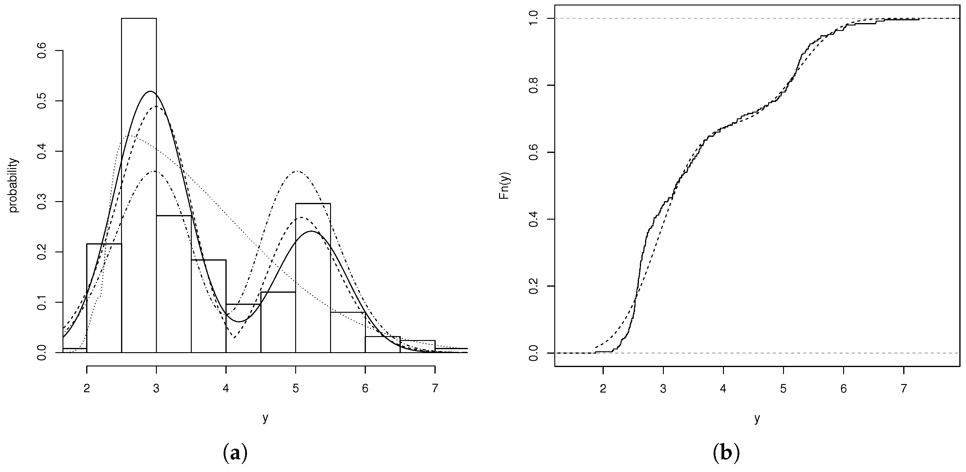
We considered a dataset from the Applied Statistics Center at the Institute of Mathematics and Statistics, University of Sao Paulo, Brazil, consisting of 250 samples of breast cancer cells from women, where the amount of DNA within the cell nucleus (ploidy) was measured. These data were previously analyzed by Siroky et al. [17] using a bimodal power-normal model. The ploidy variable exhibits bimodal asymmetric behavior, with the Hartigan and Hartigan [18,19] bimodality test yielding statistics $D=0.0399$ and a p-value = 0.0059. The ploidy data have a mean of 3.636 and variance 1.432. The data show a positive skewness of 0.452, indicating that the distribution is tilted to the right, with a longer tail in that direction. The kurtosis value of 0.865 suggests that the distribution is slightly flatter than a normal distribution, implying that the data do not exhibit extreme tails or very sharp peaks.

The following bimodal models were fitted: the bimodal skew-normal model (BSN) of Elal-Olivero et al. [4], the asymmetric power-normal bimodal model (ABPN) of Bolfarine et al. [8], the extended asymmetric double normal (ETN) of Arnold et al. [9] and the ADN model.

This study employs various information criteria to determine the best fit model for the data, including the Akaike Information Criterion (AIC), defined as $-2\widehat{\ell \left(\theta \right)}+2k$, and the Bayesian Information Criterion (BIC), given by $-2\widehat{\ell \left(\theta \right)}+klogn$. Here, $\widehat{\ell \left(\theta \right)}$ represents the estimated log-likelihood, n is the sample size, and k denotes the number of model parameters. The MLEs, along with the AIC and BIC values for the comparison of the model, are presented in

Table 3. Estimated parameters (standard errors) for the fitted models.

Estimates	BSN	ABPN	ETN	ADN
$\widehat{\xi }$	3.993 (0.046)	4.117 (0.039)	2.200 (0.034)	4.162 (0.049)
$\widehat{\eta }$	0.759 (0.023)	0.874 (0.032)	1.840 (0.085)	0.532 (0.026)
$\widehat{\lambda }$	–	−0.313 (0.063)	11.899 (3.855)	2.237 (0.015)
$\widehat{\alpha }$	5.953 (2.175)	6.721 (0.622)	13.369 (2.890)	−0.219 (0.041)
AIC	725.19	700.80	701.50	685.07
BIC	735.76	714.88	715.59	699.15

.

The results in Table 3 highlight the performance of the ADN distribution compared to other fitted models, namely BSN, ABPN, and ETN. A key observation is that the ADN model achieves the lowest AIC and BIC values, with AIC = 685.07 and BIC = 699.15. These values are approximately 15 units lower than those of the competing models, highlighting the superior ability of the ADN distribution to capture the underlying data structure.

In terms of parameter estimation, the ADN model provides reasonable estimates with smaller standard errors, particularly for $\widehat{\xi }$ and $\widehat{\eta }$, which means a stable and precise parameter fitting. The skewness parameter $\widehat{\alpha }$ and the shape parameter $\widehat{\lambda }$ further demonstrate the flexibility of the ADN model to account for asymmetry and other complex data characteristics.

These results suggest that the ADN distribution is better suited for modeling these datasets compared to the other models tested, providing a more accurate and efficient fit, as indicated by the goodness-of-fit metrics.

Figure 3a,b show the behavior of the fitted models and the empirical cumulative distribution functions for the adjusted models. These graphs reveal that the ADN model provides the best fit compared to the BSN, ABPN, and ETN models.

5.2. Illustration 2: Regression Analysis

The ADN distribution was extended to the case of having covariates that explain the response variable Y, for example, a linear regression model:

$$y_i={\beta }_0+{\beta }_1{x}_{1i}+{\beta }_2{x}_{2i}+\cdots +{\beta }_p{x}_{pi}+{\epsilon }_i,i=1,2,\dots ,n,$$

where $x_1,x_2,\dots ,x_p$ is a set of covariates, ${\beta }_0,{\beta }_1,\dots ,{\beta }_p$ is a set of unknown parameters, and ${\epsilon }_1,{\epsilon }_2,\dots ,{\epsilon }_n$ are random variables representing model errors. The most common assumption is that ${\epsilon }_i$ are random i.i.d. variables having a normal distribution with zero mean and constant variance ${\sigma }^2$.

However, this assumption does not meet standard practices. Therefore, it is assumed that ${\epsilon }_i$ are i.i.d. following a $ADN(0,\eta ,\lambda ,\alpha )$ distribution. For this example, a set of observations on various body features, such as height, weight, and body mass index, among others, is provided for all 202 athletes. These data are available at http://azzalini.stat.unipd.it/SN/ (accessed on 16 April 2022). In this context, the model

$${\mathrm{B}\mathrm{f}\mathrm{a}\mathrm{t}}_i={\beta }_0+{\beta }_1{\mathrm{b}\mathrm{m}\mathrm{i}}_i+{\beta }_2{\mathrm{l}\mathrm{b}\mathrm{m}}_i+{\epsilon }_i,$$

will be fitted for male athletes $n=102$ in this dataset, where ${\mathrm{B}\mathrm{f}\mathrm{a}\mathrm{t}}_i$ represents the percentage of body fat of the i-th athlete, and the covariates ${\mathrm{b}\mathrm{m}\mathrm{i}}_i$ and ${\mathrm{l}\mathrm{b}\mathrm{m}}_i$ denote body mass index and lean body mass, respectively, for the i-th athlete.

To obtain the estimates ${\beta }_0,{\beta }_1,{\beta }_2,\eta ,\lambda ,\alpha$ for the model, we maximize the log-likelihood function (11), where $z_i=({\mathrm{B}\mathrm{f}\mathrm{a}\mathrm{t}}_i-{\beta }_0-{\beta }_1{\mathrm{b}\mathrm{m}\mathrm{i}}_i-{\beta }_2{\mathrm{l}\mathrm{b}\mathrm{m}}_i)/\eta$.

Regression models will be fitted assuming normal errors, skew-normal errors, and ADN errors. The MLEs along with the corresponding AIC and BIC comparison criteria are provided in

Table 4. MLE for the Australian athletes’ data and the corresponding standard errors (in parentheses), as well as AIC and BIC values.

Estimates	N	SN	ADN
${\widehat{\beta }}_0$	−7.206 (2.148)	−5.183 (2.661)	0.818  (1.788)
${\widehat{\beta }}_1$	$-0.0831\left(0.038\right)$	−0.043 (0.038)	−0.088 (0.031)
${\widehat{\beta }}_2$	0.948 (0.136)	0.628 (0.203)	0.794  (0.125)
$\widehat{\eta }$	5.930 (0.580)	3.672 (0.399)	1.800  (0.184)
$\widehat{\lambda }$	–	–	2.408  (0.231)
$\widehat{\alpha }$	–	3.508 (1.497)	−0.744 (0.151)
AIC	477.02	462.36	453.01
BIC	487.51	480.11	468.76

.

According to these comparison criteria, the best regression model is the one with ADN errors, followed by the model with skew-normal errors and, finally, the one with normal errors.

To further validate the model fit quality beyond information criteria (AIC and BIC), we conducted a formal goodness-of-fit test on the residuals of the fitted models. Specifically, we apply the Anderson–Darling test, which is particularly sensitive to deviations in the tails of the distribution, making it suitable for assessing asymmetric distributions.

The Anderson–Darling test was implemented using goftest package in R version 4.3.2. [20]. This test examines whether residuals follow the assumed distribution, with higher p values indicating a better agreement with the theoretical distribution.

Table 5. Anderson–Darling test results for model residuals.

Statistic	N	SN	ADN
Anderson–Darling	15.0890	1.5720	0.3912
p-value	0.0000	0.1602	0.8571

presents the Anderson–Darling test statistics and the corresponding p values for the residuals of each fitted model.

The results provide strong evidence supporting the ADN model as the most appropriate choice. The normal error model is decisively rejected (p-value $=0.0000$), while the skew-normal model shows marginal acceptability (p-value $=0.1602$). In contrast, the ADN model produces a high p ($0.8571$), indicating that the null hypothesis of ADN-distributed errors cannot be rejected. This finding strongly supports the previous conclusion based on information criteria that the ADN distribution provides the best fit to the data. These results further validate the superiority of the ADN distribution in modeling the data structure, particularly in capturing the asymmetric and potentially bimodal characteristics present in the dataset.

To identify atypical observations and/or model misalignment, we analyzed the transformation of the martingale residual, rMTi, proposed by Barros et al. [21]. These residuals are defined by

$$rM{T}_i=\mathrm{sgn}\left(r{M}_i\right){(-2[r{M}_i+{\kappa }_{i}log({\kappa }_i-r{M}_i)])}^{1/2},i=1,2,\cdots ,n,$$

where $r{M}_i={\kappa }_i+log(S(e_i,\widehat{\theta }))$ is the martingale residual proposed by Ortega et al. [22], where ${\kappa }_i=0,1$ indicates whether the observation i-th is censored or not, respectively, $\mathrm{sgn}\left(r{M}_i\right)$ denotes the sign of $r{M}_i$, and $S(e_i;\widehat{\theta })$ represents the survival function evaluated at $e_i$ (standardized classical residuals), where $\widehat{\theta }$ represents the MLE for $\theta$.

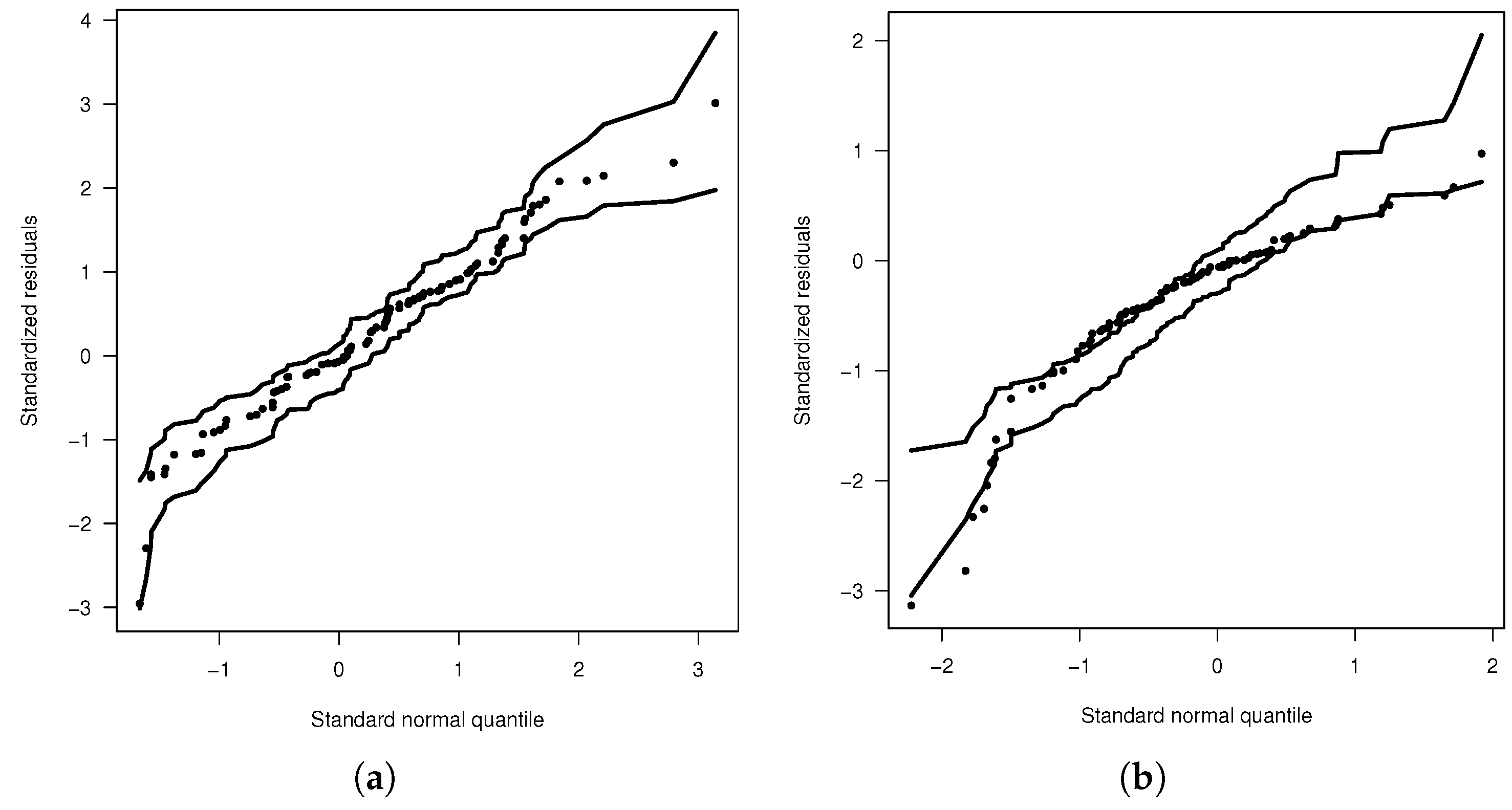
To verify the assumptions of the model, error distribution, fit issues, and presence of potential outliers, we generated confidence bands through simulations for the martingale residuals, which are known in the diagnostic analysis literature as envelopes.

Figure 4a,b display the envelope plots for the fitted models. These plots reveal that the ADN regression model provides the best fit compared to the SN regression model. Recall that envelope plots also help confirm the validity of the model’s distributional assumptions and identify influential observations. From the envelope plot for the ADN model, it is clear that the model with ADN errors does not exhibit influential observations or distributional assumption issues.

6. Discussions and Conclusions

The asymmetric double normal distribution represents a significant advancement in statistical modeling, addressing the inherent limitations of the normal distribution in representing asymmetry and multimodality in real-life data. By incorporating shape and skewness parameters, it provides remarkable flexibility to accommodate both unimodal and bimodal forms, while elegantly maintaining the normal distribution as a special case. The comprehensive simulation study validates the robustness of the maximum likelihood estimators for the proposed model, confirming their desirable asymptotic behavior and the reliability of the associated statistical inference procedures. These findings strongly support the applicability of the method in practical scenarios where precise parameter estimation is essential for appropriate modeling of complex phenomena. The empirical applications presented in this work convincingly demonstrate the practical advantages of the proposed distribution over alternative models in both the distribution fitting and regression analysis contexts. For example, as illustrated in Figure 3 and further detailed in Table 3, the visual fit of the ADN model to bimodal ploidy data, along with its superior AIC and BIC values compared to competing models, such as BSN, ABPN, and ETN, provides compelling empirical evidence of its improved ability to capture complex data structures.

The model’s ability to simultaneously capture asymmetry and bimodality in data, while maintaining parsimonious parameterization, offers a powerful tool for data analysis. In the context of linear regression, the incorporation of asymmetric double normal errors substantially expands the scope of application of linear models in scenarios where the classical normality assumptions are inadequate. Thorough residual diagnostics confirm that the proposed model satisfies distributional assumptions appropriately, thus providing a more flexible and realistic framework for analyzing data with complex patterns that are prevalent in various scientific disciplines.

Despite its flexibility, the ADN model, like any statistical model, has certain limitations and specific domains of optimal applicability. The analytical determination of precise conditions for bimodality solely in terms of $\lambda$ and $\alpha$ can be complex, often necessitating numerical exploration, as discussed in Remark 4. Although the ADN distribution can model a wide array of skewed and bimodal shapes, for datasets exhibiting extremely heavy tails or more than two distinct modes, further extensions of the model or alternative specialized distributions might be more appropriate. Furthermore, parameter estimation relies on numerical optimization techniques; While found to be generally robust in our studies, these methods can, in some instances, be sensitive to starting values or encounter convergence issues with particularly challenging datasets or very small sample sizes. A formal investigation tail behavior of the model and a comparative study against specific heavy-tailed distributions are also warranted for future work. Furthermore, while this paper focuses on the frequentist MLE approach, the development and comparison of alternative estimation methods, such as a comprehensive Bayesian estimation framework for the ADN model, represent a valuable avenue for future research that could provide additional insight into parameter uncertainty and model robustness.

These considerations represent natural directions for future research, along with the promising possibility of being extended to trimodal models and the application of the model to non-Gaussian time-series analysis. The solid statistical foundation of this proposal, which includes a rigorous derivation of moments, characteristic functions, and stochastic representations, together with its empirical validation across different datasets, ensures its robustness and broad applicability in diverse fields, such as biomedicine, economics, and engineering. For practitioners facing univariate data that exhibit skewness and potential bimodality, the ADN model offers a clear workflow: initial data visualization to assess these features, followed by model fitting via MLE to estimate its parameters. Interpretation of these parameters, particularly $\lambda$ for overall shape and $\alpha$ for skewness, coupled with a model comparison using criteria such as AIC/BIC, allows for a nuanced understanding and robust modeling of the data.

Consequently, this flexible distribution is well positioned to gain significant traction in modeling complex phenomena, providing statisticians and data analysts with a powerful tool to explore intricate data structures. Future work will extend this distribution to a wider variety of scenarios and explore additional theoretical refinements to further enhance its flexibility and utility in statistical practice.