Enhancing Land Cover Classification: Fuzzy Similarity Approach Versus Random Forest

Abstract

This study presents a comparative analysis of two advanced classification techniques applied to Landsat 8 and Sentinel-2 imagery. The first technique is based on the combined use of Tversky’s fuzzy similarity and Mamdani-type fuzzy inference, specifically designed to handle transition zones—areas characterized by gradual shifts in land cover, such as from vegetation to suburban environments. The second approach is based on the Random Forest algorithm. After performing the ranking of spectral, textural, and geometric features using the fuzzy approach, a fuzzy system based on Tversky’s fuzzy similarity was developed. This system enables a more adaptive and nuanced classification of different land cover classes, including water bodies, forests, and cultivated areas. The results indicate that the proposed fuzzy approach slightly outperforms the Random Forest method in handling mixed land cover regions and reducing classification uncertainties, achieving overall accuracies of 98.5% for Sentinel-2 and 96.7% for Landsat 8.

1. Introduction

The increasing accessibility of satellite imagery is crucial for analyzing the dynamics of ecosystems [1,2]. Satellite-based vegetation mapping provides vital information on the interaction between the natural environment and human activities, playing a key role in development programs and land-use monitoring [3,4]. Furthermore, this kind of imagery also enables the analysis of key parameters that affect the quality of life, such as water stress, urban heat islands [5], pollution, and natural disasters (e.g., floods and wildfires) [6], facilitating emergency response [7,8,9]. The processing of such data is becoming increasingly complex as spatial resolution improves. Recently, two main methodologies for remote sensing image analysis have emerged: knowledge-driven techniques [10,11,12,13,14,15,16,17,18,19,20] and data-driven approaches [21,22,23,24,25,26,27,28,29,30,31,32,33,34]. Additionally, recent advances in satellites, sensors, and analytical techniques, such as Object-Based Image Analysis (OBIA), are expanding remote sensing applications, enhancing both precision and effectiveness [35]. OBIA and multiresolution segmentation represent advanced methodologies that improve satellite image classification by overcoming the limitations of pixel-based approaches through a hierarchical structure capable of managing multiscale relationships and integrating spatial and spectral data. However, OBIA proves less effective when dealing with images affected by uncertainties and inaccuracies, where spectral variability, gradual transitions between classes, and heterogeneous data quality can compromise classification performance, reducing its reliability in complex scenarios.

To predict ecosystem dynamics, it is essential to develop predictive models that integrate remote sensing data and advanced analysis to simulate the evolution of natural environments in response to anthropogenic and climatic factors, supporting sustainable management strategies. These models require accurate and adaptable land classification, especially in heterogeneous landscapes, where data variability and imprecision pose significant challenges [36,37]. In fact, the precise classification of remotely sensed images (i.e., differentiating between water bodies and forest rather than cultivated areas) is essential for correctly identifying land use and environmental parameters, ensuring reliable analyses, and improving the precision of predictions on ecological dynamics and anthropogenic impacts [38,39].

In recent years, the classification of remote sensing images has made significant progress thanks to the integration of deep learning (DL) [40,41], convolutional neural networks (CNNs) [42,43], and supervised [44,45] and unsupervised learning methods [46,47]. These techniques excel in extracting complex features, enabling detailed classifications even in heterogeneous contexts [48]. Their strength lies in processing large volumes of data, leveraging spectral, spatial, and temporal information to identify relevant patterns [49]. Additionally, the use of pre-trained architectures and generative models has improved the generalization of predictions, overcoming the scarcity of labeled data [50].

Despite their success, these approaches have critical limitations, including difficulty in handling uncertainties and inaccuracies in images caused by atmospheric variability, non-uniform resolution, and gradual transitions between land use classes [51,52].

Random Forest (RF), among the supervised learning techniques for remote sensing image classification, represents an area of ongoing exploration [53,54,55]. With its ability to process large amounts of data, RF is widely used in image classification, including applications in environmental monitoring and land cover mapping, providing high accuracy and interpretability of complex data [56,57].

However, RF, while being a robust and effective model for image classification, has limitations in areas affected by uncertainty and imprecision. Since it operates with crisp classifications, it assigns each pixel to a single class without considering the possibility of gradual transitions or overlaps between categories, leading to errors in regions with blurred boundaries, such as transition areas between different land cover types or images affected by atmospheric variability and noise. Moreover, their reliance on a fixed set of features can reduce their ability to adapt to data with high spectral ambiguity, compromising classification accuracy in complex scenarios.

To address these challenges, research is exploring fuzzy approaches that handle uncertainties and ambiguities by assigning a membership degree to each pixel, ranging from 0 to 1. This method overcomes the rigidity of traditional classifications, thereby improving the representation of gradual transitions and spectral overlaps [58,59,60].

However, despite the numerous fuzzy classifiers proposed for satellite images, none of them utilize Fuzzy Similarity (FS) computations [61,62] to group similar images into homogeneous classes by identifying a single representative image for each class, from which features summarizing the main characteristics of the images belonging to that class can be extracted. This approach provides a dual advantage: it reduces computational complexity and enhances scalability, making classification more intuitive and efficient. The classification of an unknown area would be performed by comparing, through FS, the extracted features with those of the representative classes, making the process faster and more interpretable [63,64]. Furthermore, relying on synthetic representatives ensures greater robustness against uncertainties and inaccuracies, improving the ability to capture gradual transitions between categories [65].

The study we present in this work aligns with the objectives of the National Recovery and Resilience Plan (PNRR), which promotes sustainable development by integrating innovative technologies for environmental monitoring and protection. The proposed method addresses the challenges posed by incomplete and uncertain data, providing an intelligent system that enhances the understanding of ecosystem dynamics and increases resilience to environmental impacts.

The remainder of this paper is organized as follows: Section 2 details the Landsat 8 and Sentinel-2 images exploited in this work. Section 3 provides a mathematical representation of the images based on their spectral bands. Section 4 and Section 5 offer an overview of the calculation and representation of both reflectance and spectral bands, as well as georeferencing. Section 6 describes the extraction of the images’ features. Section 7 and Section 8 describe the preprocessing phase and the fuzzy ranking based on FS. Section 9 describes the experimental database, while the results of the fuzzy ranking approach are discussed in Section 10. The key findings related to image classification are presented in Section 11 and Section 12. Section 13 presents the results of the image classification using RF. In Section 14 and Section 15, some evaluations regarding computational complexities are presented. Finally, the conclusion and future perspectives complete this work.

2. Landsat 8 and Sentinel-2A: A Brief Overview

2.1. Regarding Landsat 8 Imagery

Landsat 8 images exhibit high spectral resolution and radiometric stability, ensuring reliable and consistent information over time. The satellite is equipped with two main instruments: the Operational Land Imagery (OLI) instrument, which captures data across nine spectral bands, making it effective for analyzing vegetation, soil, and water resources, and the Thermal Infrared Sensor (TIRS), which collects data in two thermal infrared (TIR) bands to study land surface temperature, detect Urban Heat Islands (UHIs), and monitor soil moisture variations. The images acquired by the Landsat 8 satellite contain detailed information due to the division of the electromagnetic spectrum into different bands, each with specific applications in environmental and surface analysis. Their specific technical characteristics and applications are outlined in

Table 1. Spectral characteristics and applications of Landsat 8 bands. The table provides the wavelength range, spatial resolution, and primary uses of each band. Visible and near-infrared bands support vegetation and land cover analysis, shortwave infrared detects moisture content, and thermal infrared enables temperature mapping and soil moisture estimation. The panchromatic band enhances image sharpness, while coastal aerosol and cirrus bands aid in atmospheric corrections.

Band	Description	Wavelength (Micron)	Spatial Resolution (m)	Use
Band 1	Coastal Aerosol	0.43–0.45	30	Imaging shallow water, detecting fine atmospheric particles (dust and smoke)
Band 2	Blue	0.45–0.51	30	Bathymetric mapping, distinguishing soil from vegetation, deciduous from coniferous vegetation
Band 3	Green	0.53–0.59	30	Peak vegetation, assessing plant vigor
Band 4	Red	0.64–0.67	30	Discriminates vegetation slopes
Band 5	Near InfraRed	0.85–0.88	30	Biomass content, shorelines
Band 6	SWIR1	1.57–1.65	30	Discriminates moisture content of soil and vegetation, penetrates thin clouds
Band 7	SWIR2	2.1–2.29	30	Improved moisture content of soil and vegetation, penetrates thin clouds
Band 8	Pancromatic (PAN)	0.50–0.68	15	Meter resolution, sharper image definition
Band 9	Cirrus	1.36–1.38	30	Improved detection of cirrus cloud contamination
Band 10	Thermal Infra-Red 1	1060–11.19	100	Thermal mapping, estimated soil moisture
Band 11	Thermal Infra-Red 2	11.50–12.51	100	Improved thermal mapping, estimated soil moisture

[66].

The images acquired by the Landsat 8 satellite provide a clear representation of different types of land cover. As illustrated in Figure 1, spectral analysis effectively distinguishes water surfaces, forested areas, and cultivated lands, highlighting differences in reflectance across various bands of the electromagnetic spectrum. These spectral characteristics are essential for land use classification and environmental monitoring.

2.2. Regarding Sentinel-2 Imagery

Sentinel-2A images, acquired by the MSI multispectral sensor within the ESA Copernicus program, are essential for global surface monitoring. Operational since 2015 and complemented by Sentinel-2B, the satellite provides high-resolution data in terms of spectral, spatial, and temporal resolution, supporting applications ranging from agriculture to environmental management and urban planning. The 13 spectral bands of Sentinel-2A cover the visible, near-infrared, and shortwave infrared regions. Visible bands enable natural color visualization, while the red-edge and near-infrared bands are crucial for vegetation and chlorophyll monitoring. SWIR bands detect soil and vegetation moisture and distinguish surface materials, making them vital for environmental studies. Spatial resolution varies by band: 10 m for visible and near-infrared, 20 m for red-edge and SWIR, and 60 m for atmospheric and cloud detection bands. This balance between detail and coverage allows for both high-precision and large-scale analyses. With a five-day revisit frequency, Sentinel-2A enables the continuous monitoring of dynamic phenomena, including land cover changes, crop growth, and environmental impacts. Images are divided into $100\times 100$ km² tiles, georeferenced in the UTM system, and available at processing levels 1C (TOA) and 2A (BOA) to optimize spectral and environmental analysis. Data are freely accessible through platforms such as the Copernicus Open Access Hub and cloud services, with advanced analysis performed using ESA’s SNAP and GIS software 11.0.0. Global coverage from 84° S to 84° N, with repeated acquisitions every five days, ensures reliable observations of ecosystems and natural resources. Thanks to its sun-synchronous orbit at 786 km and tandem operation with Sentinel-2B, the system guarantees high revisit frequency, providing continuous data for scientific, environmental, and land management applications (for details, see

Table 2. Spectral characteristics and applications of Sentinel-2 bands. The table details the central wavelength, bandwidth, spatial resolution, and primary uses. Visible and red-edge bands support vegetation and land cover analysis, near-infrared aids biomass and coastal mapping, and shortwave infrared helps assess soil moisture, snow, and cloud differentiation. Additional bands improve atmospheric corrections by detecting aerosols, water vapor, and cirrus clouds.

Band	${\mathit{\lambda }}_{\mathit{b}}$ (nm)	$\mathbf{\Delta }\mathit{b}$	Resolution (m)	Use
B01	443	20	60	Aerosol detection
B02 (blue)	490	65	10	Distinguishes soil and vegetation, aiding in the mapping of forests and artificial elements. Dispersed by the atmosphere, it illuminates shaded areas better than longer wavelengths and penetrates clear water more effectively. Chlorophyll absorption makes plants appear darker.
B03 (green)	560	35	10	Provides strong contrast between clear and turbid water, penetrating well into clear water. Highlights oil on water surfaces and vegetation, reflecting more green light than other visible colors, while artificial structures remain distinguishable.
B04 (red)	665	30	10	Strongly reflected by dead foliage, it helps identify vegetation, soils, and urban areas. It has limited water penetration and low reflectance in chlorophyll-rich live foliage.
B05 (red-edge)	705	15	20	Vegetation classification.
B06	740	15	20	Vegetation classification.
B07	783	20	20	Vegetation classification.
B08 (Near InfraRed—NIR)	842	115	10	The near-infrared band is ideal for mapping coastlines, analyzing biomass, and monitoring vegetation.
B08A	865	20	20	Vegetation classification.
B09	945	20	60	Water vapor detection.
B10	1375	30	60	Cirrus detection.
B11 (SWIR1)	1610	90	20	Measures soil and vegetation moisture, distinguishes vegetation types, and differentiates snow from clouds, but has limited cloud penetration.
B12 (SWIR2)	2190	180	20	Measures soil and vegetation moisture, provides contrast between vegetation types, and distinguishes snow from clouds, but has limited cloud penetration.

). The images acquired by the Sentinel-2 satellite offer a detailed representation of various land cover types. As shown in Figure 2, spectral analysis allows for the effective differentiation of water bodies, forested regions, and cultivated areas by highlighting variations in reflectance across multiple spectral bands [67,68].

Remark 1.

While Sentinel-2 provides 13 spectral bands as listed in Table 2, only 11 were used in this study. Bands B01 (443 nm, aerosol detection) and B10 (1375 nm, cirrus detection) were excluded due to their limited contribution to land cover classification. Both bands are primarily designed for atmospheric correction and are available at lower spatial resolution (60 m). Their exclusion was also supported by the fuzzy similarity-based feature ranking, which indicated low discriminative relevance. This choice improved computational efficiency while maintaining classification accuracy in the fuzzy inference process.

3. Mathematical Modeling and Spectral Representation of Images

A Landsat 8 satellite image is here represented as a three-dimensional tensor:

$$I(x,y,b_i),x=1,\dots ,N_x;y=1,\dots ,N_y;i=1,\dots 9.$$

(1)

where $I(x,y,b)$ is the reflectance value at the pixel with coordinates $(x,y)$ in band b, $N_x$ and $N_y$ represent the spatial dimensions of the image in pixels, and $b_i$ is the spectral band index (ranging from 1 to 9).

Each band $b_i$ is defined by the central wavelength ${\lambda }_b$ (nm), which indicates the band’s position in the electromagnetic spectrum; the bandwidth $\mathrm{\Delta }{\lambda }_b$, which specifies the range of captured wavelengths; and the spatial resolution $R_b$, which defines the pixel size.

Similarly, for Sentinel-2 images, we can write

$$\widehat{I}(x,y,{\widehat{b}}_j),x=1,\dots ,{\widehat{N}}_x;y=1,\dots ,{\widehat{N}}_y;j=1,\dots ,11.$$

(2)

where ${\widehat{N}}_x$ and ${\widehat{N}}_y$ represent the spatial dimensions of the image in pixels.

Spatial Resolution and Scale Transformation

Landsat 8 has nine bands, including one with a higher spatial resolution (panchromatic) of 15 m, seven bands with a spatial resolution of 30 m, and one thermal band with a coarser resolution of 60 m. In contrast, Sentinel-2 provides 10m pixels for bands 2, 3, and 4 (visible bands) and band 8 (NIR), while bands 5, 6, 7, 8A, 11, and 12 have a spatial resolution of 20 m. Finally, bands 1, 9, and 10 are available at 60 m resolution. The actual dimensions of a band $b_i$ in Landsat 8 images can be expressed as $N_{x,b_i}={\displaystyle \frac{N_x}{R_{b_i}}}$, $N_{y,b_i}={\displaystyle \frac{N_y}{R_{b_i}}}$. Similarly, for Sentinel-2 images, it is appropriate to write ${\widehat{N}}_{x,{\widehat{b}}_j}={\displaystyle \frac{{\widehat{N}}_x}{{\widehat{R}}_{{\widehat{b}}_j}}}$ and ${\widehat{N}}_{y,{\widehat{b}}_j}={\displaystyle \frac{{\widehat{N}}_y}{{\widehat{R}}_{{\widehat{b}}_j}}}$, where $R_{b_i}$ and ${\widehat{R}}_{{\widehat{b}}_j}$ represent the spatial resolutions of the images for each band, respectively.

Remark 2.

In the mathematical model in which $b_i=1,\dots ,9$ is written, the index refers only to the OLI bands, which were those used for the classification and spectral analysis in the present study. The TIRS thermal bands (bands 10 and 11), although listed for completeness in the technical description of the sensor, were not used in the data processing due to their different nature (thermal) and lower spatial resolution.

4. Reflectance: Computation and Visualization for Remote Sensing Analysis

Reflectance is defined as the fraction of light energy reflected by the Earth’s surface relative to the incident energy. Sentinel-2 captures radiance values, which are subsequently converted into TOA (Top-Of-Atmosphere) or BOA (Bottom-Of-Atmosphere) reflectance. TOA reflectance is calculated as

$${\rho }_{TOA}(x,y,b_i)={\displaystyle \frac{\pi ·L_i(x,y,b_i)}{E_{si}\left(b_i\right)·cos\left({\theta }_s\right)}},{\widehat{\rho }}_{TOA}(x,y,{\widehat{b}}_j)={\displaystyle \frac{\widehat{\pi }·{\widehat{L}}_j(x,y,{\widehat{b}}_j)}{{\widehat{E}}_{sj}\left(b\right)·cos\left({\widehat{\theta }}_{sj}\right)}}$$

(3)

where $L_i(x,y,b)$ and ${\widehat{L}}_j(x,y,b)$ represent the spectral radiance measured by the sensor in band $b_i$ and ${\widehat{b}}_j$ at pixel $(x,y)$ (in W/m²/sr/μm). Additionally, $E_{si}\left(b_i\right)$ and ${\widehat{E}}_{sj}\left(b_j\right)$ are the respective solar irradiance values at the central wavelength ${\lambda }_b$ (in W/m²/μm) for Landsat 8 and Sentinel-2 images. The solar zenith angle (rad) for Landsat 8 and Sentinel-2 images is denoted as ${\theta }_{s_i}$ and ${\widehat{\theta }}_{s_j}$, respectively. Finally, $\pi$ and $\widehat{\pi }$ represent the respective normalization factors. BOA reflectance was corrected for atmospheric effects and computed using radiative transfer models for both Landsat 8 and Sentinel-2 images as follows:

$${\rho }_{BOA}(x,y,b_i)={\displaystyle \frac{{\rho }_{TOA}(x,y,b_i)-T_{atm}\left(b_i\right)}{1+S_{atm}\left(b_i\right)}}$$

(4)

$${\widehat{\rho }}_{BOA}(x,y,{\widehat{b}}_j)={\displaystyle \frac{{\widehat{\rho }}_{TOA}(x,y,{\widehat{b}}_j)-{\widehat{T}}_{atm}\left({\widehat{b}}_j\right)}{1+{\widehat{S}}_{atm}\left({\widehat{b}}_j\right)}}$$

(5)

where $T_{atm}\left(b_i\right)$ and ${\widehat{T}}_{atm}\left({\widehat{b}}_j\right)$ represent the respective atmospheric contributions to radiance, while $S_{atm}\left(b_i\right)$ and ${\widehat{S}}_{atm}\left({\widehat{b}}_j\right)$ denote the corresponding atmospheric scattering components.

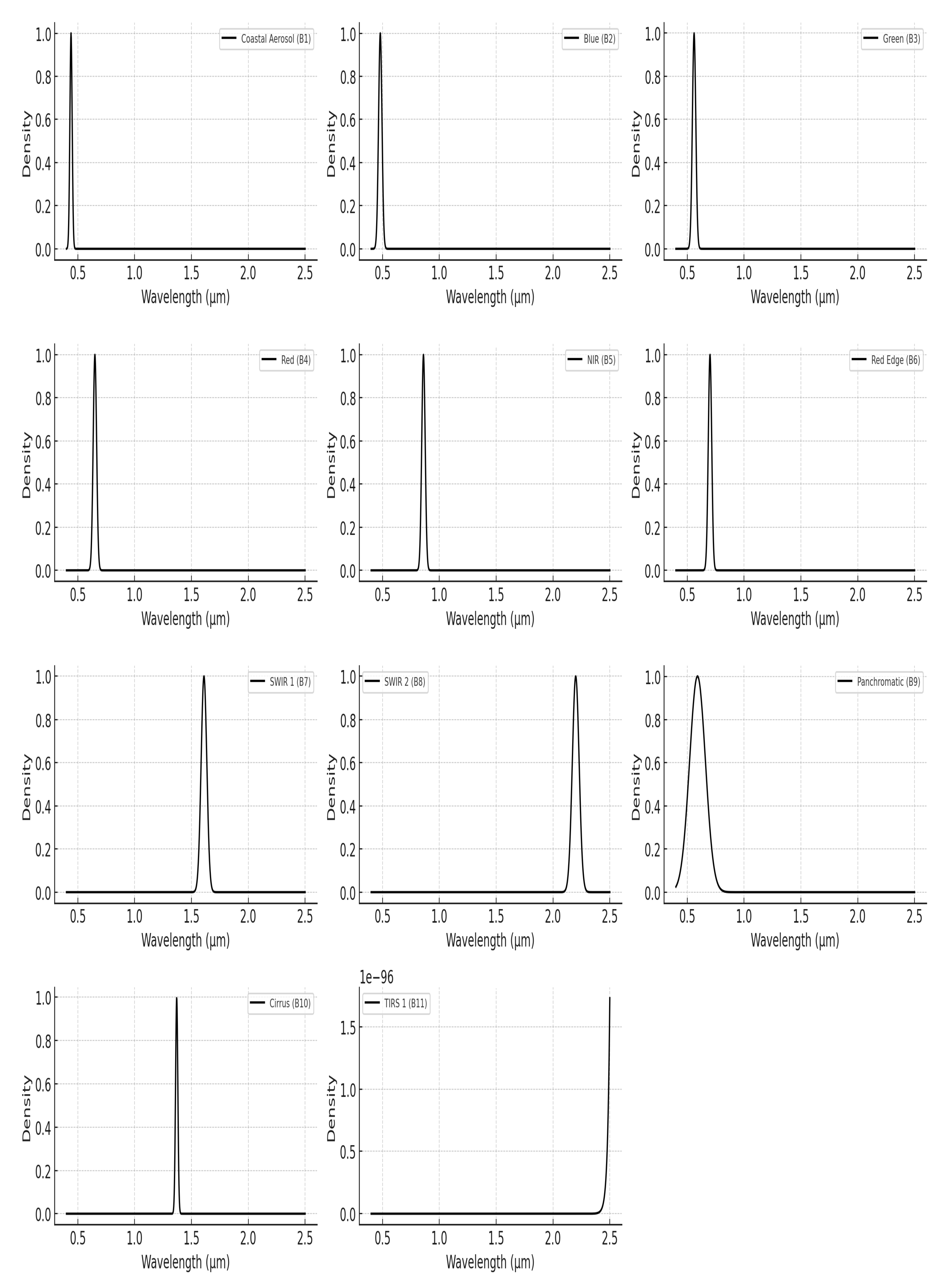
5. Spectral Bands and Georeferencing for Precision Earth Observation

Each band, b and $\widehat{b}$, served a specific purpose, as highlighted in Table 1 and Table 2. Each pixel, $I(x,y,b)$ and $\widehat{I}(x,y,b)$, was georeferenced within a Universal Transverse Mercator (UTM) coordinate system. The actual coordinates $(E_{x,b_i},N_{x,b_i})$$(E_{y,b_i},N_{y,b_i})$ and $({\widehat{E}}_{x,{\widehat{b}}_j},{\widehat{N}}_{x,{\widehat{b}}_j})$$({\widehat{E}}_{y,{\widehat{b}}_i},{\widehat{N}}_{y,{\widehat{b}}_j})$ of a pixel were computed as

$$E_{x,b_i}={\left(E_0\right)}_{x,b_i}+x·R_{b_i},N_{x,b_i}={\left(N_0\right)}_{x,b_i}-y·R_{b_i}$$

(6)

for Landsat 8, while, for Sentinel-2, Equation (6) was specified as

$${\widehat{E}}_{x,{\widehat{b}}_j}={\left({\widehat{E}}_0\right)}_{x,{\widehat{b}}_j}+x·{\widehat{R}}_{b_i},N_{x,b_j}={\left({\widehat{N}}_0\right)}_{x,{\widehat{b}}_j}-y·{\widehat{R}}_{{\widehat{b}}_j},$$

(7)

where $({\left(E_0\right)}_{x,b_i},{\left(N_0\right)}_{x,b_i})$ and $({\left({\widehat{E}}_0\right)}_{x,{\widehat{b}}_j},{\left({\widehat{N}}_0\right)}_{x,{\widehat{b}}_j})$ are the UTM coordinates of the upper-left corner of the scene, while $R_{b_i}$ and ${\widehat{R}}_{{\widehat{b}}_j}$ represent the spatial resolutions of bands $b_i$ and ${\widehat{b}}_j$, respectively.

6. Feature Extraction

The extracted features were divided into four main categories: spectral, textural, geometric, and temporal.

6.1. Spectral Features (SF)

These describe the radiometric response of spectral bands and help identify and classify different types of land cover. In this work, we used the following spectral features:

6.1.1. MeanReflectance

For bands $b_i$ and ${\widehat{b}}_j$, the mean reflectance could be computed as

$${\overline{R}}_{b_i}={\displaystyle \frac{1}{N_{x,b_i}\times N_{y,b_i}}}\sum _{s=1}^{N_{x,b_i}}\sum _{r=1}^{N_{y,b_i}}{R}_{b_i}(r,s),{\overline{\widehat{R}}}_{b_j}={\displaystyle \frac{1}{{\widehat{N}}_{x,{\widehat{b}}_j}\times {\widehat{N}}_{y,{\widehat{b}}_j}}}\sum _{n=1}^{{\widehat{N}}_{x,{\widehat{b}}_j}}\sum _{m=1}^{{\widehat{N}}_{y,{\widehat{b}}_j}}{\widehat{R}}_{{\widehat{b}}_j}(m,n)$$

(8)

where ${\overline{R}}_{b_i}$ and ${\overline{\widehat{R}}}_{{\widehat{b}}_j}$ represent the reflectance values in the respective bands, $b_i$ and ${\widehat{b}}_j$.

6.1.2. Band Ratios

Band ratios highlight spectral differences. Mathematically, ${\overline{R}}_{b_{hk}}={\displaystyle \frac{R_{b_h}}{R_{b_k}}}$, $h,k=1,\dots ,9$ and ${\overline{\widehat{R}}}_{{\widehat{b}}_{zt}}={\displaystyle \frac{{\widehat{R}}_{{\widehat{b}}_z}}{{\widehat{R}}_{{\widehat{b}}_t}}}$ with $z,t=1,\dots 11$.

6.1.3. Spectral Indices

Spectral bands from both Landsat 8 and Sentinel-2 images could be mathematically combined to derive indices. One of the most useful indices was the Normalized Difference Moisture Index (NDMI), which was defined as

$$NDMI={\displaystyle \frac{{\rho }_{BOA}(x,y,b_5)-{\rho }_{BOA}(x,y,b_6)}{{\rho }_{BOA}(x,y,b_5)+{\rho }_{BOA}(x,y,b_6)}}$$

(9)

for Landsat 8 images, while, for Sentinel-2 images, it was expressed as

$$\widehat{NDMI}={\displaystyle \frac{{\widehat{\rho }}_{BOA}(x,y,{\widehat{b}}_8)-{\widehat{\rho }}_{BOA}(x,y,{\widehat{b}}_{11})}{{\widehat{\rho }}_{BOA}(x,y,{\widehat{b}}_8)+{\widehat{\rho }}_{BOA}(x,y,{\widehat{b}}_{11})}}.$$

(10)

6.2. Textural Features

These describe the spatial distribution of pixel values, useful for analyzing the structure and homogeneity of a region.

Co-Occurrence Matrix of Gray Levels (COMGL)

COMGL measures the frequency at which pairs of pixels with specific intensities appear in a given spatial relationship. For both types of images, intensity values needed to be quantized into G gray levels as follows:

$$I^{\prime }(x,y,b_i)=\left[{\displaystyle \frac{I(x,y,b_i)-min\left\{I(x,y,b_i)\right\}}{max\left\{I(x,y,b_i)\right\}-min\left\{I(x,y,b_i)\right\}}}\times (G-1)\right],$$

(11)

$${\widehat{I}}^{\prime }(x,y,b_j)=\left[{\displaystyle \frac{\widehat{I}(x,y,b_j)-min\left\{\widehat{I}(x,y,b_j)\right\}}{max\left\{\widehat{I}(x,y,b_j)\right\}-min\left\{\widehat{I}(x,y,b_j)\right\}}}\times (G-1)\right].$$

(12)

A spatial relationship was defined by a vector whose components were denoted as $\mathrm{\Delta }x$ and $\mathrm{\Delta }y$. The most common configurations were horizontal $(\mathrm{\Delta }x,\mathrm{\Delta }y)=(1,0)$, vertical $(\mathrm{\Delta }x,\mathrm{\Delta }y)=(0,1)$, main diagonal $(\mathrm{\Delta }x,\mathrm{\Delta }y)=(1,1)$, and secondary diagonal $(\mathrm{\Delta }x,\mathrm{\Delta }y)=(1,-1)$. For Landsat 8 images, for each band $b_i$, we computed the matrix

$$P_{b_i}(\delta ,\eta )=\left|\{(x,y):I^{\prime }(x,y,b_i)=\delta \mathrm{and}{I}^{\prime }(x+\mathrm{\Delta }x,y+\mathrm{\Delta }y,b_i)=\eta \}\right|$$

(13)

while, for Sentinel-2 images, for each band ${\widehat{b}}_j$, we defined

$${\widehat{P}}_{{\widehat{b}}_j}(\widehat{\delta },\widehat{\eta })=\left|\{(x,y):{\widehat{I}}^{\prime }(x,y,{\widehat{b}}_j)=\widehat{\delta }\mathrm{and}{\widehat{I}}^{\prime }(x+\mathrm{\Delta }x,y+\mathrm{\Delta }y,{\widehat{b}}_j)=\eta \}\right|.$$

(14)

From both (13) and (14), to obtain the corresponding probability distributions, we constructed their normalized forms:

$$P_{b_i}^{\mathrm{norm}}(\delta ,\eta )={\displaystyle \frac{P_{b_i}(\delta ,\eta )}{{\sum }_{\delta =0}^{G-1}{\sum }_{\eta =0}^{G-1}{P}_{b_i}(\delta ,\eta )}},{\widehat{P}}_{{\widehat{b}}_j}^{\mathrm{norm}}(\widehat{\delta },\widehat{\eta })={\displaystyle \frac{{\widehat{P}}_{{\widehat{b}}_j}(\widehat{\delta },\widehat{\eta })}{{\sum }_{\delta =0}^{G-1}{\sum }_{\eta =0}^{G-1}{\widehat{P}}_{{\widehat{b}}_j}(\widehat{\delta },\widehat{\eta })}}.$$

(15)

Both in (15) enabled comparable statistical analysis across different spectral bands. Specifically, from the COMGL matrices of each band, for both image types, we computed the following textural features:

• Contrast, which measured the difference between adjacent pixel intensities:

  $${\mathrm{Contrast}}_{b_i}=\sum _{\delta ,\eta }{P}_{b_i}^{\mathrm{norm}}(\delta ,\eta ){(\delta -\eta )}^2,{\widehat{\mathrm{Contrast}}}_{{\widehat{b}}_i}=\sum _{\widehat{\delta },\widehat{\eta }}{\widehat{P}}_{{\widehat{b}}_j}^{\mathrm{norm}}(\widehat{\delta },\widehat{\eta }){(\widehat{\delta }-\widehat{\eta })}^2.$$

  (16)
• Energy, which measured the uniformity of value distribution:

  $${\mathrm{Energy}}_{b_i}(\delta ,\eta )=\sum _{\delta ,\eta }{\left[P_{b_i}^{\mathrm{norm}}(\delta ,\eta )\right]}^2,{\widehat{\mathrm{Energy}}}_{{\widehat{b}}_j}(\widehat{\delta },\widehat{\eta })=\sum _{\widehat{\delta },\widehat{\eta }}{\left[{\widehat{P}}_{{\widehat{b}}_j}^{\mathrm{norm}}(\widehat{\delta },\widehat{\eta })\right]}^2.$$

  (17)
• Homogeneity, which measured the (non-fuzzy) similarity between adjacent values:

  $${\mathrm{Hom}}_{b_i}(\delta ,\eta )=\sum _{\delta ,\eta }{\displaystyle \frac{P_b^{\mathrm{norm}}(\delta ,\eta )}{1+|\delta -\eta |}},{\widehat{\mathrm{Hom}}}_{{\widehat{b}}_j}(\widehat{\delta },\widehat{\eta })=\sum _{\widehat{\delta },\widehat{\eta }}{\displaystyle \frac{{\widehat{P}}_{b_j}^{\mathrm{norm}}(\widehat{\delta },\widehat{\eta })}{1+|\widehat{\delta }-\widehat{\eta }|}}.$$

  (18)
• Entropy, which measured the randomness of the intensity value distribution:

  $$\begin{array}{c}\hfill {\mathrm{Entropy}}_{b_i}(\delta ,\eta )=-\sum _{\delta ,\eta }{P}_{b_i}^{\mathrm{norm}}(\delta ,\eta )·{log}_2\left[P_{b_i}^{\mathrm{norm}}(\delta ,\eta )\right],\\ \hfill {\widehat{\mathrm{Entropy}}}_{{\widehat{b}}_j}(\widehat{\delta },\widehat{\eta })=-\sum _{\widehat{\delta },\widehat{\eta }}{\widehat{P}}_{{\widehat{b}}_j}^{\mathrm{norm}}(\widehat{\delta },\widehat{\eta })·{log}_2\left[{\widehat{P}}_{{\widehat{b}}_j}^{\mathrm{norm}}(\widehat{\delta },\widehat{\eta })\right].\end{array}$$

  (19)

6.3. Geometric Features

These describe the geometric properties of segmented regions in images, such as shape, size, and proportions. These features are crucial for comprehending the morphology of target areas and enhancing image classification. The primary geometric features included perimeter, $\mathrm{Perimeter}={\sum }_{i\in \mathrm{edge}\left(R\right)}1$, where $\mathrm{edge}\left(R\right)$ represents the pixels forming the boundary of a region. The area was given by $A={\sum }_{i\in R}1$, where R is the set of pixels forming the region.

To quantify how closely a region resembled a circle and how elongated a region was, we used the compactness and eccentricity indices.

$$\mathrm{Compactness}={\displaystyle \frac{4\pi \mathrm{Area}}{{\left(\mathrm{Perimeter}\right)}^2}},\mathrm{Eccentricity}=\sqrt{1-{\displaystyle \frac{{\left(\mathrm{ax}\right)}^2}{{\left(\mathrm{Ax}\right)}^2}}}$$

(20)

$\mathrm{Compactness}\to 1$ indicated a more circular shape, while ax and Ax were the minor and major semi-axes, respectively.

Remark 3.

Although the features described here provide valuable insights, they can be computationally expensive, especially for real-time applications. Thus, ranking their importance is essential, and given that images often contain uncertainties, a fuzzy-based ranking approach is recommended.

7. Fuzzy-Based Feature Ranking for Remote Sensing Analysis (FFR)

FFR ranks features by importance while accounting for data uncertainty. The proposed method integrates fuzzy sets (FSs) to assess feature similarity in a fuzzy manner, utilizing a fuzzy inference system (FIS) that applies fuzzy rule-based computations to perform ranking. This approach assigns a fuzzy score to each feature, ordering them by relevance to the classification task.

We introduce the following definitions.

Definition 1.

For Landsat 8 images, given a set of features,

$$F_{b_i}=\{F_{b_i}^1,F_{b_i}^2,\dots ,F_{b_i}^{\zeta }\dots ,F_{b_i}^p\}$$

(21)

we define a function Z on this set as follows:

$$Z:F_{b_i}\to {[0,1]}^p,$$

(22)

such that for every $\forall F_{b_i}^{\zeta }\in F$, with $\zeta =1,\dots ,p$, a number ${\gamma }_{b_i}^{\zeta }\in [0,1]$ is assigned. The closer ${\gamma }_{b_i}^{\zeta }$ is to 1, the greater the importance of $F_{\zeta }$. Conversely, if ${\gamma }_{b_i}^{\zeta }$ approaches 0, its significance decreases.

Definition 2.

Similarly, for Sentinel-2 images, if the set of features is denoted by

$${\widehat{F}}_{{\widehat{b}}_j}=\{{\widehat{F}}_{{\widehat{b}}_j}^1,{\widehat{F}}_{{\widehat{b}}_j}^2,\dots ,{\widehat{F}}_{{\widehat{b}}_j}^{\zeta }\dots ,{\widehat{F}}_{{\widehat{b}}_j}^p\}$$

(23)

we define a function $\widehat{Z}$ on this set as follows:

$$\widehat{Z}:{\widehat{F}}_{b_j}\to {[0,1]}^p.$$

(24)

Similarly, for every $\forall {\widehat{F}}_{b_j}^{\zeta }\in {\widehat{F}}_{{\widehat{b}}_j}$, with $\zeta =1,\dots ,p$, a number ${\widehat{\gamma }}_{b_j}^{\zeta }\in [0,1]$ is assigned. If ${\widehat{\gamma }}_{b_j}^{\zeta }$ approaches 1, this indicates high importance of ${\widehat{F}}_{b_j}^{\zeta }$, whereas, if it nears 0, the considered feature loses significance.

To correctly define the functions (23) and (24), we need to normalize each feature (because different orders of magnitude can characterize them) and then fuzzify them appropriately.

Normalization and Fuzzification

Relating to Landsat 8 and Sentinel-2 images, with features $F_{b_i}^{\zeta }$ and ${\widehat{F}}_{{\widehat{b}}_j}^{\zeta }$, which have different value scales, we normalize them within the range $[0,1]$ as follows:

$${\left(F_{b_i}^{\zeta }\right)}^{\mathrm{norm}}={\displaystyle \frac{F_{b_i}^{\zeta }-min\left(F_{b_i}\right)}{max\left(F_{b_i}\right)-min\left(F_{b_i}\right)}},{\left({\widehat{F}}_{{\widehat{b}}_j}^{\zeta }\right)}^{\mathrm{norm}}={\displaystyle \frac{{\widehat{F}}_{{\widehat{b}}_j}^{\zeta }-min\left({\widehat{F}}_{{\widehat{b}}_j}\right)}{max\left({\widehat{F}}_{{\widehat{b}}_j}\right)-min\left({\widehat{F}}_{{\widehat{b}}_j}\right)}}$$

(25)

where $min\left(F_{b_i}\right)$ and $max\left(F_{b_i}\right)$ represent the minimum and maximum values of the feature $F_{b_i}$, while $max\left({\widehat{F}}_{{\widehat{b}}_j}\right)$ and $min\left({\widehat{F}}_{{\widehat{b}}_j}\right)$ are the maximum and minimum values for ${\widehat{F}}_{{\widehat{b}}_j}^{\zeta }$.

Each ${\left(F_{b_i}^{\zeta }\right)}^{\mathrm{norm}}$ and ${\left({\widehat{F}}_{{\widehat{b}}_j}^{\zeta }\right)}^{\mathrm{norm}}$, to ensure a smooth transition of membership values over the possible value range, is converted into its corresponding fuzzy membership degree (low, medium, high) using Gaussian functions:

$$\mu {\left({\left(F_{b_i}^{\zeta }\right)}^{\mathrm{norm}}\right)}_{\mathrm{low}}=e^{-{\displaystyle \frac{{({\left(F_{b_i}^{\zeta }\right)}^{\mathrm{norm}}-a_1)}^2}{2{\sigma }^2}}},\mu {\left({\left(F_{b_i}^{\zeta }\right)}^{\mathrm{norm}}\right)}_{\mathrm{medium}}=e^{-{\displaystyle \frac{{({\left(F_{b_i}^{\zeta }\right)}^{\mathrm{norm}}-a_2)}^2}{2{\sigma }^2}}}$$

(26)

$$\mu {\left({\left(F_{b_i}^{\zeta }\right)}^{\mathrm{norm}}\right)}_{\mathrm{high}}=e^{-{\displaystyle \frac{{({\left(F_{b_i}^{\zeta }\right)}^{\mathrm{norm}}-a_3)}^2}{2{\sigma }^2}}},\mu {\left({\left({\widehat{F}}_{{\widehat{b}}_j}^{\zeta }\right)}^{\mathrm{norm}}\right)}_{\mathrm{low}}=e^{-{\displaystyle \frac{{({\left({\widehat{F}}_{{\widehat{b}}_j}^{\zeta }\right)}^{\mathrm{norm}}-e_1)}^2}{2{\sigma }^2}}}$$

(27)

$$\mu {\left({\left({\widehat{F}}_{{\widehat{b}}_j}^{\zeta }\right)}^{\mathrm{norm}}\right)}_{\mathrm{medium}}=e^{-{\displaystyle \frac{{({\left({\widehat{F}}_{{\widehat{b}}_j}^{\zeta }\right)}^{\mathrm{norm}}-e_2)}^2}{2{\sigma }^2}}},\mu {\left({\left({\widehat{F}}_{{\widehat{b}}_j}^{\zeta }\right)}^{\mathrm{norm}}\right)}_{\mathrm{high}}=e^{-{\displaystyle \frac{{({\left({\widehat{F}}_{{\widehat{b}}_j}^{\zeta }\right)}^{\mathrm{norm}}-e_3)}^2}{2{\sigma }^2}}}.$$

(28)

The parameter setting for the shape of Gaussian functions is performed by computing the minimum, maximum, and mean of the normalized features for the central values, while the standard deviation is chosen to cover the observed range evenly. The selection of $\sigma$ can depend on the feature’s dispersion, with a common approach being the use of the standard deviation of the normalized distribution. This ensures that the Gaussian curve spans the range between the minimum and maximum while maintaining a smooth transition.

Remark 4.

The choice to set the shape parameters based on the minimum, mean, and maximum is driven by the fact that these are intuitive and straightforward formulations that effectively adapt to the distribution of features, making the corresponding fuzzy membership functions easily interpretable as “low”, “medium”, and “high”. Setting σ as 1/6 of the range ensures a smooth transition between different membership functions without excessive overlap or gaps.

8. Fuzzy Ranking Features: An Approach Based on Tversk’s Formulation

In this work, we adopted the TFS because it provides a symmetric similarity measure, which flexibly adjusts for differences between fuzzy quantities and better adapts to geospatial data, often characterized by uncertainties and gradual transitions between classes.

8.1. The Advantage of TFS: Enhancing Feature Similarity in Remote Sensing

Unlike traditional FS metrics, which treat differences between fuzzy sets symmetrically, the TFS flexibly adjusted the relative importance of differences among spectral, textural, and geometric features extracted from the Landsat 8 and Sentinel-2 images. This approach highlighted the most relevant characteristics in the ranking, adapting to the discriminative capacity of features in detecting specific phenomena such as vegetation, soil moisture, or anthropogenic elements. Additionally, it reduced the impact of redundant or irrelevant features, improving selection efficiency. Since Landsat 8 and Sentinel-2 images have bands with different resolutions and cover distinct wavelength ranges, the ability to customize the weight of differences between features enabled more accurate selection, preventing less significant characteristics from affecting the final ranking.

Computationally, TFS integrated seamlessly with the fuzzy framework used for ranking, ensuring consistency between the fuzzification phase and feature comparison. The use of Gaussian membership functions to model features in a nuanced manner enhanced the quality of rankings, making the selection process more robust. Furthermore, TFS is particularly effective in handling imbalanced feature sets, preventing underrepresented features from being excessively penalized. This ensured a more balanced selection and greater reliability in classifying Landsat 8 and Sentinel-2 features.

The TFS quantifies how “close” a fuzzified feature is to a target feature. Based on its classical definition and indicating with $\omega \in \{\mathrm{low},\mathrm{medium},\mathrm{high}\}$, the Tversky FS for Landsat 8 images takes the following form:

$$\begin{array}{c}\hfill S(\mu {\left({\left(F_{b_i}^{\zeta }\right)}^{\mathrm{norm}}\right)}_{\omega },\mu {\left({\left(C_{b_i}^{\zeta }\right)}^{\mathrm{norm}}\right)}_{\omega })=(1+{\displaystyle \frac{{\chi }_1|\mu {\left({\left(F_{b_i}^{\zeta }\right)}^{\mathrm{norm}}\right)}_{\omega }-\mu {\left({\left(C_{b_i}^{\zeta }\right)}^{\mathrm{norm}}\right)}_{\omega }|}{|\mu {\left({\left(F_{b_i}^{\zeta }\right)}^{\mathrm{norm}}\right)}_{\omega }\cap \mu {\left({\left(C_{b_i}^{\zeta }\right)}^{\mathrm{norm}}\right)}_{\omega }|}}+\\ \hfill +{\displaystyle \frac{{\chi }_2|\mu {\left({\left(C_{b_i}^{\zeta }\right)}^{\mathrm{norm}}\right)}_{\omega }-\mu {\left({\left(F_{b_i}^{\zeta }\right)}^{\mathrm{norm}}\right)}_{\omega }|}{|\mu {\left({\left(F_{b_i}^{\zeta }\right)}^{\mathrm{norm}}\right)}_{\omega }\cap \mu {\left({\left(C_{b_i}^{\zeta }\right)}^{\mathrm{norm}}\right)}_{\omega }|}}{)}^{-1}\in [0,1]\end{array}$$

(29)

where $\mu {\left({\left(C_{b_i}^{\zeta }\right)}^{\mathrm{norm}}\right)}_{\omega }$ represents the fuzzified target feature, while

$$|\mu {\left({\left(F_{b_i}^{\zeta }\right)}^{\mathrm{norm}}\right)}_{\omega }\cap \mu {\left({\left(C_{b_i}^{\zeta }\right)}^{\mathrm{norm}}\right)}_{\omega }|=min\left(\mu {\left({\left(F_{b_i}^{\zeta }\right)}^{\mathrm{norm}}\right)}_{\omega },\mu {\left({\left(C_{b_i}^{\zeta }\right)}^{\mathrm{norm}}\right)}_{\omega }\right),$$

(30)

$$|\mu {\left({\left(F_{b_i}^{\zeta }\right)}^{\mathrm{norm}}\right)}_{\omega }-\mu {\left({\left(C_{b_i}^{\zeta }\right)}^{\mathrm{norm}}\right)}_{\omega }|=max\left(0,\mu {\left({\left(F_{b_i}^{\zeta }\right)}^{\mathrm{norm}}\right)}_{\omega }-\mu {\left({\left(C_{b_i}^{\zeta }\right)}^{\mathrm{norm}}\right)}_{\omega }\right),$$

(31)

$$|\mu {\left({\left(C_{b_i}^{\zeta }\right)}^{\mathrm{norm}}\right)}_{\omega }-\mu {\left({\left(F_{b_i}^{\zeta }\right)}^{\mathrm{norm}}\right)}_{\omega }|=max\left(0,\mu {\left({\left(C_{b_i}^{\zeta }\right)}^{\mathrm{norm}}\right)}_{\omega }-\mu {\left({\left(F_{b_i}^{\zeta }\right)}^{\mathrm{norm}}\right)}_{\omega }\right).$$

(32)

Finally, the parameters ${\chi }_1$ and ${\chi }_2$ regulate the weighting of penalties for fuzzy differences.

Similarly, for Sentinel-2 images, Equation (29) specializes as follows:

$$\begin{array}{c}\hfill S(\mu {\left({\left({\widehat{F}}_{{\widehat{b}}_j}^{\zeta }\right)}^{\mathrm{norm}}\right)}_{\omega },\mu {\left({\left(C_{b_i}^{\zeta }\right)}^{\mathrm{norm}}\right)}_{\omega })=\end{array}$$

(33)

$$\begin{array}{c}\hfill =(1+{\displaystyle \frac{{\widehat{\chi }}_1|\mu {\left({\left({\widehat{F}}_{{\widehat{b}}_j}^{\zeta }\right)}^{\mathrm{norm}}\right)}_{\omega }-\mu {\left({\left(C_{b_i}^{\zeta }\right)}^{\mathrm{norm}}\right)}_{\omega }|}{|\mu {\left({\left({\widehat{F}}_{{\widehat{b}}_j}^{\zeta }\right)}^{\mathrm{norm}}\right)}_{\omega }\cap \mu {\left({\left(C_{b_i}^{\zeta }\right)}^{\mathrm{norm}}\right)}_{\omega }|}}+\\ \hfill +{\displaystyle \frac{{\widehat{\chi }}_2|\mu {\left({\left(C_{b_i}^{\zeta }\right)}^{\mathrm{norm}}\right)}_{\omega }-\mu {\left({\left({\widehat{F}}_{{\widehat{b}}_j}^{\zeta }\right)}^{\mathrm{norm}}\right)}_{\omega }|}{|\mu {\left({\left({\widehat{F}}_{{\widehat{b}}_j}^{\zeta }\right)}^{\mathrm{norm}}\right)}_{\omega }\cap \mu {\left({\left(C_{b_i}^{\zeta }\right)}^{\mathrm{norm}}\right)}_{\omega }|}}{)}^{-1}\in [0,1],\end{array}$$

(34)

where, of course, ${\widehat{\chi }}_1$ and ${\widehat{\chi }}_2$ regulate the respective weighting of penalties for fuzzy differences, while

$$|\mu {\left({\left({\widehat{F}}_{{\widehat{b}}_j}^{\zeta }\right)}^{\mathrm{norm}}\right)}_{\omega }\cap \mu {\left({\left(C_{b_i}^{\zeta }\right)}^{\mathrm{norm}}\right)}_{\omega }|=min\left(\mu {\left({\left({\widehat{F}}_{{\widehat{b}}_j}^{\zeta }\right)}^{\mathrm{norm}}\right)}_{\omega },\mu {\left({\left(C_{b_i}^{\zeta }\right)}^{\mathrm{norm}}\right)}_{\omega }\right),$$

(35)

$$|\mu {\left({\left({\widehat{F}}_{{\widehat{b}}_j}^{\zeta }\right)}^{\mathrm{norm}}\right)}_{\omega }-\mu {\left({\left(C_{b_i}^{\zeta }\right)}^{\mathrm{norm}}\right)}_{\omega }|=max\left(0,\mu {\left({\left({\widehat{F}}_{{\widehat{b}}_j}^{\zeta }\right)}^{\mathrm{norm}}\right)}_{\omega }-\mu {\left({\left(C_{b_i}^{\zeta }\right)}^{\mathrm{norm}}\right)}_{\omega }\right),$$

(36)

$$|\mu {\left({\left(C_{b_i}^{\zeta }\right)}^{\mathrm{norm}}\right)}_{\omega }-\mu {\left({\left({\widehat{F}}_{{\widehat{b}}_j}^{\zeta }\right)}^{\mathrm{norm}}\right)}_{\omega }|=max\left(0,\mu {\left({\left(C_{b_i}^{\zeta }\right)}^{\mathrm{norm}}\right)}_{\omega }-\mu {\left({\left({\widehat{F}}_{{\widehat{b}}_j}^{\zeta }\right)}^{\mathrm{norm}}\right)}_{\omega }\right).$$

(37)

Remark 5.

The assignment of parameters ${\chi }_1$, ${\chi }_2$, ${\widehat{\chi }}_1$, and ${\widehat{\chi }}_2$ depends on the importance given to the differences between fuzzy values. Specifically, if one aims to penalize the difference in feature values relative to the target class more strongly, it is advisable to assign a higher value to ${\chi }_1$ and ${\widehat{\chi }}_1$. If the target class exhibits significant internal variability or ambiguity, assigning a higher weight to ${\chi }_2$ and ${\widehat{\chi }}_2$ is beneficial. These values emphasize the differences between the features of the images to be classified and the target class while maintaining a certain symmetry in the similarity calculation.

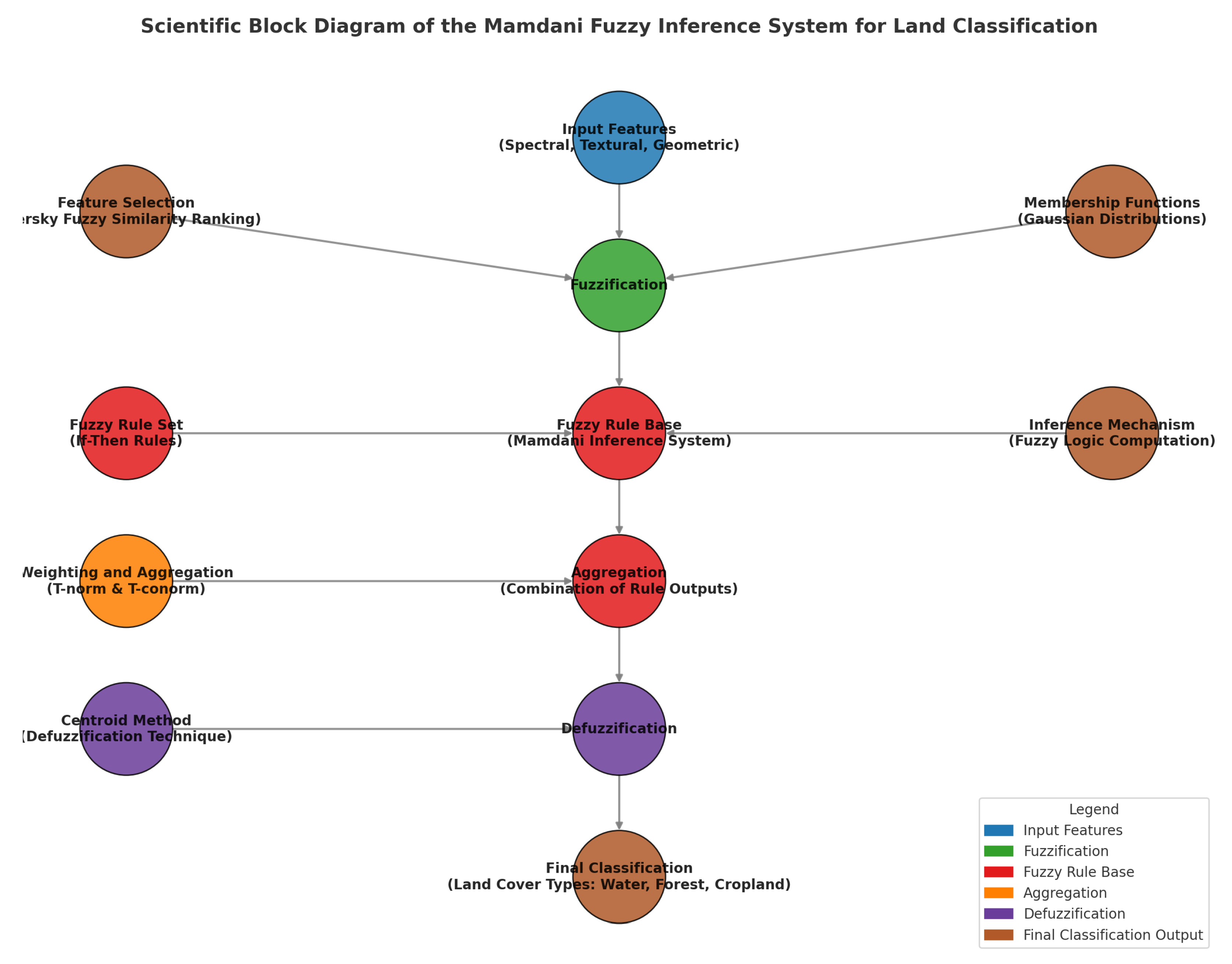
8.2. Enhanced Fuzzy Feature Ranking: Integrating FS & FIS for Optimal Classification

The FS value is integrated into an FIS, which takes as inputs, in addition to FS, the variance of the features, $\sigma \left(\mu {\left({\left(F_{b_i}^{\zeta }\right)}^{\mathrm{norm}}\right)}_{\omega }\right)$, and the uncertainty,

$$U\left(\mu {\left({\left(F_{b_i}^{\zeta }\right)}^{\mathrm{norm}}\right)}_{\omega }\right))=1-max\left(\mu {\left({\left(F_{b_i}^{\zeta }\right)}^{\mathrm{norm}}\right)}_{\omega }\right)),\omega \in \{\mathrm{low},\mathrm{medium},\mathrm{high}\}$$

(38)

These values are used to activate the following fuzzy rules:

• IF $S(\mu {\left({\left(F_{b_i}^{\zeta }\right)}^{\mathrm{norm}}\right)}_{\omega },\mu {\left({\left(C_{b_i}^{\zeta }\right)}^{\mathrm{norm}}\right)}_{\omega })$ is high AND $\sigma \left(\mu {\left({\left(F_{b_i}^{\zeta }\right)}^{\mathrm{norm}}\right)}_{\omega }\right)$ is low
  AND $U\left(\mu {\left({\left(F_{b_i}^{\zeta }\right)}^{\mathrm{norm}}\right)}_{\omega }\right))$ is low THEN ${\left(F_{b_i}^{\zeta }\right)}^{\mathrm{norm}}$ is very important;
• IF $S(\mu {\left({\left(F_{b_i}^{\zeta }\right)}^{\mathrm{norm}}\right)}_{\omega },\mu {\left({\left(C_{b_i}^{\zeta }\right)}^{\mathrm{norm}}\right)}_{\omega })$ is medium AND $\sigma \left(\mu {\left({\left(F_{b_i}^{\zeta }\right)}^{\mathrm{norm}}\right)}_{\omega }\right)$ is medium
  AND $U\left(\mu {\left({\left(F_{b_i}^{\zeta }\right)}^{\mathrm{norm}}\right)}_{\omega }\right))$ is low THEN ${\left(F_{b_i}^{\zeta }\right)}^{\mathrm{norm}}$ is moderately important;
• IF $S(\mu {\left({\left(F_{b_i}^{\zeta }\right)}^{\mathrm{norm}}\right)}_{\omega },\mu {\left({\left(C_{b_i}^{\zeta }\right)}^{\mathrm{norm}}\right)}_{\omega })$ is low AND $\sigma \left(\mu {\left({\left(F_{b_i}^{\zeta }\right)}^{\mathrm{norm}}\right)}_{\omega }\right)$ is high
  AND $U\left(\mu {\left({\left(F_{b_i}^{\zeta }\right)}^{\mathrm{norm}}\right)}_{\omega }\right))$ is low THEN ${\left(F_{b_i}^{\zeta }\right)}^{\mathrm{norm}}$ is unimportant.

For Sentinel-2 images, the rules for Landsat 8 images are modified to account for the specific spectral characteristics of the MSI, as follows:

• IF $S(\mu {\left({\left({\widehat{F}}_{{\widehat{b}}_j}^{\zeta }\right)}^{\mathrm{norm}}\right)}_{\omega },\mu {\left({\left(C_{b_i}^{\zeta }\right)}^{\mathrm{norm}}\right)}_{\omega })$ is high AND $\sigma \left(\mu {\left({\left({\widehat{F}}_{{\widehat{b}}_j}^{\zeta }\right)}^{\mathrm{norm}}\right)}_{\omega }\right)$ is low
  AND $U\left(\mu {\left({\left({\widehat{F}}_{{\widehat{b}}_j}^{\zeta }\right)}^{\mathrm{norm}}\right)}_{\omega }\right))$ is low THEN ${\left({\widehat{F}}_{{\widehat{b}}_j}^{\zeta }\right)}^{\mathrm{norm}}{)}_{\omega }$ is very important;
• IF $S(\mu {\left({\left({\widehat{F}}_{{\widehat{b}}_j}^{\zeta }\right)}^{\mathrm{norm}}\right)}_{\omega },\mu {\left({\left(C_{b_i}^{\zeta }\right)}^{\mathrm{norm}}\right)}_{\omega })$ is medium AND $\sigma \left(\mu {\left({\left({\widehat{F}}_{{\widehat{b}}_j}^{\zeta }\right)}^{\mathrm{norm}}\right)}_{\omega }\right)$ is medium
  AND $U\left(\mu {\left({\left({\widehat{F}}_{{\widehat{b}}_j}^{\zeta }\right)}^{\mathrm{norm}}\right)}_{\omega }\right))$ is high THEN ${\left({\widehat{F}}_{{\widehat{b}}_j}^{\zeta }\right)}^{\mathrm{norm}}{)}_{\omega }$ is moderately important;
• IF $S(\mu {\left({\left({\widehat{F}}_{{\widehat{b}}_j}^{\zeta }\right)}^{\mathrm{norm}}\right)}_{\omega },\mu {\left({\left(C_{b_i}^{\zeta }\right)}^{\mathrm{norm}}\right)}_{\omega })$ is low AND $\sigma \left(\mu {\left({\left(F_{b_i}^{\zeta }\right)}^{\mathrm{norm}}\right)}_{\omega }\right)$ is high
  AND $U\left(\mu {\left({\left({\widehat{F}}_{{\widehat{b}}_j}^{\zeta }\right)}^{\mathrm{norm}}\right)}_{\omega }\right))$ is high THEN ${\left({\widehat{F}}_{{\widehat{b}}_j}^{\zeta }\right)}^{\mathrm{norm}}{)}_{\omega }$ is unimportant.

The activation degree of each rule is determined as the minimum among the membership degrees of the antecedents, following the Mamdani approach based on the minimum operator (t-norm). The fuzzy implication involves truncating the output set at the activation level of the corresponding rule, followed by aggregating the truncated outputs using the max operator (t-conorm). Defuzzification is then performed using the centroid method, applying the Guldino–Pappus formulation [69,70]. Finally, by sorting the defuzzified values in descending order, the feature ranking is obtained. Figure 3 depicts the flowchart of the Mamdani FIS approach.

9. Comprehensive Analysis of the Available Database

The images were selected based on spectral variability, geographic diversity, and radiometric quality. Spectral variability was ensured by including areas with different land covers and atmospheric conditions. Geographic diversity was maintained by selecting images from various regions, enhancing the model’s robustness. Radiometric quality was preserved by using images with low noise and applied atmospheric corrections.

The database was divided into two sets: training and testing, both containing images representing three main categories: water bodies, forested areas, and cultivated lands. For training, the Landsat 8 database included 55 water images, 60 forest images, and 70 cultivated land images, ensuring coverage of diverse environmental conditions. The Sentinel-2 training database comprised 60 water images, 65 forest images, and 70 cultivated land images, covering a broad range of atmospheric and geographic scenarios.

The testing set was constructed using images distinct from those in the training set to assess the model’s ability to generalize to new data. For Landsat 8, the testing set comprised 20 water images, 25 forest images, and 30 cultivated land images, ensuring that the geographic distribution and atmospheric conditions of the training set were maintained. For Sentinel-2, the testing set comprised 25 water images, 30 forest images, and 35 cultivated land images, ensuring a balanced representation of environmental conditions. For details, see

Table 3. Landsat 8: spatial distribution of training and testing images across diverse land cover categories.

	Water	Forest	Cultivated Area
Training Database	55 × 9	60 × 9	70 × 9
Testing Database	20 × 9	25 × 9	30 × 9

and

Table 4. Sentinel-2: optimized distribution of training and testing images across varied land cover classes for enhanced classification accuracy.

	Water	Forest	Cultivated Area
Training Database	60 × 11	65 × 11	70 × 11
Testing Database	25 × 11	30 × 11	35 × 11

.

10. Advanced Insights from Fuzzy Ranking of Features

By applying the normalization and fuzzification procedure, the following target feature classes were obtained for the Landsat 8 images. Figure 4, Figure 5 and Figure 6 illustrate the spectral feature targets after normalization and fuzzification for water bodies, forests, and croplands, respectively. Particularly, Figure 4 shows the normalized Gaussian membership curves for each spectral band of Landsat 8 derived for the water body class. These curves highlight the distinct spectral behavior of water surfaces, which typically exhibit low reflectance in the visible red and near-infrared bands and relatively higher reflectance in the blue band, corresponding to the typical absorption and reflection properties of water. This spectral configuration is instrumental in distinguishing water from vegetated or built-up areas during classification. Moreover, Figure 5 presents the corresponding Gaussian distributions for forested areas, highlighting the strong reflectance in the near-infrared band and the moderate absorption in the red and blue bands. These patterns are characteristic of healthy vegetation due to chlorophyll absorption and high internal leaf reflectance. The comparison between Figure 4 and Figure 5 underlines the differences in spectral responses between water and forested land covers, which were crucial for the accuracy of the fuzzy classification model.

Figure 7, Figure 8 and Figure 9 illustrate the normalized and fuzzified Gaussian curves corresponding to the textural features of water bodies, forests, and cultivated areas. Similarly, the representative Gaussians for the target features of Sentinel-2 images were generated but are not displayed due to space constraints.

10.1. Optimized Feature Ranking Using a Fuzzy Approach: Insights from Landsat 8 Images

For Landsat 8 images of water bodies, the feature ranking obtained through the fuzzy approach confirmed the expected importance order from the literature, highlighting the predominance of spectral features, followed by textural features, and, finally, geometric features. NDMI proved to be the most effective index for water identification, effectively separating vegetation from soil. Reflectance in band 2 highlighted water’s low absorption of blue light, while band 3 helped distinguish between clear and turbid water. Band 4, due to red light absorption, indicated water presence when reflectance values were low. Additionally, band 5 aided in identifying water surfaces through reduced reflectance values. Finally, the SWIR1 and SWIR2 bands were essential for distinguishing water from wet soil or ice. Among textural features, homogeneity was the most significant, as it reflected the uniform structure of water surfaces compared to soil and vegetation. Energy, although slightly less critical, helped detect pixel value variations and distinguish between smooth surfaces and turbulent areas. Contrast played a role in identifying water boundaries with other surfaces, while entropy helped detect areas with variable water conditions, such as coasts or lakes with high sedimentation. Finally, geometric features completed the ranking. Compactness was helpful in distinguishing rivers from lakes or marshes, while perimeter provided information about water-land boundaries. The area was crucial for quantifying the extent of water bodies, while eccentricity differentiated the linear shapes of rivers from the more regular forms of lakes.

The feature ranking for Landsat 8 images highlighted variations across different land cover categories while confirming the predominance of spectral features over textural and geometric ones. For forested areas, NDMI remained the most significant feature, quantifying vegetation vigor, with high values indicating dense, healthy forests and low values corresponding to sparse vegetation or bare soil. Band 5 reflectance monitored biomass content, while Band 4 reflectance, absorbed by chlorophyll, distinguished active vegetation from soil. Bands 6 and 7 captured leaf structure variations and water stress, whereas SWIR1 and SWIR2 assessed vegetation moisture, detected wildfires, and differentiated forests from bare soil.

Among textural features, homogeneity was the most relevant for distinguishing forest types and canopy density, followed by contrast, which separated dense vegetation from degraded zones. Energy provided insights into repetitive patterns, while entropy was functional only for highly heterogeneous vegetation.

Geometric features primarily mapped forest extent and fragmentation, with area being the most crucial parameter. Perimeter aided in identifying transitions between forested and non-forested areas, compactness helped distinguish dense forests from fragmented landscapes, and eccentricity differentiated compact forests from elongated formations, such as riparian zones.

For cultivated areas, NDVI was the most effective index for distinguishing healthy crops from bare soil or stressed vegetation. Bands 5 and 4 reflectance helped differentiate crops from soil and assess vegetation density, while Band 3 reflectance identified crop colors. SWIR1 and SWIR2 determined soil and plant moisture levels, which are crucial for monitoring water stress.

Textural features were essential in distinguishing uniform crops, such as wheat and maize, from more heterogeneous plantations like orchards and vineyards. Homogeneity ranked highest, followed by energy, which detected repetitive patterns in crops. Contrast and entropy differentiated monocultures from mixed-crop areas or naturally vegetated zones.

Finally, geometric features described the spatial arrangement of cultivated fields. Area defined crop extent, perimeter highlighted field boundaries, compactness distinguished well-defined agricultural plots from irregular fields, and eccentricity differentiated elongated fields from more compact ones. The summarized results are presented in

Table 5. Fuzzy-based feature ranking for Landsat 8 images: key spectral, textural, and geometric attributes across different land cover types.

Water Bodies	Forests	Cultivated Areas
NDMI	NDMI	NDMI
Reflectance in Band 2	Reflectance in Band 5	Reflectance in Band 5
Reflectance in Band 4	Reflectance in Band 4	Reflectance in Band 4
Reflectance in Band 5	Reflectance in Band 3	Reflectance in Band 3
SWIR1 and SWIR2	Reflectance in Bands 6 and 7	Reflectance in Band 2
	SWIR1 and SWIR2	SWIR1 and SWIR2
Homogeneity	Homogeneity	Homogeneity
Energy	Contrast	Energy
Contrast	Energy	Contrast
Entropy	Entropy	Entropy
Compactness	Area	Area
Perimeter	Perimeter	Perimeter
Area	Compactness	Compactness
Eccentricity	Eccentricity	Eccentricity

.

10.2. Fuzzy-Based Feature Ranking for Sentinel-2: Prioritizing Key Attributes Across Land Cover Classes

For Sentinel-2 water body images, the fuzzy ranking highlighted NDMI as the most significant feature for distinguishing water from land and vegetation, followed by Band 2 reflectance, which identified submerged areas. Band 3 reflectance differentiated between clear and turbid water, while Band 4 helped define water–land boundaries. Additionally, reflectance in Bands 8 and 11 separated water from wetlands and moist soils, whereas Band 12 distinguished water from wet soil and detected suspended pollutants or debris.

Regarding textural features, homogeneity remained the most relevant, similar to Landsat 8 images. Energy, contrast, and entropy helped assess water texture uniformity, differentiate water bodies from land, and detect variations in water color and reflectance, respectively.

For geometric features, the ranking prioritized area, followed by perimeter, compactness, and eccentricity, maintaining consistency with the Landsat 8 ranking.

In Sentinel-2 forested areas, spectral features played a fundamental role in identifying vegetation, assessing health status, and distinguishing forests from other land covers. NDVI held primary importance, with high values indicating dense, healthy forests and low values signaling sparse or degraded vegetation. Band 8 reflectance was crucial for distinguishing forests from bare soil due to vegetation’s strong near-infrared reflectance, while Band 4 reflectance highlighted active vegetation through chlorophyll absorption. Band 3 reflectance aided in differentiating vegetation types and detecting plant stress. The red-edge bands were essential for monitoring vegetation density and structural changes, while the SWIR1 and SWIR2 bands helped assess water stress, detect forest degradation, and separate vegetation from other materials.

For agricultural areas, NDVI remained the primary index for evaluating crop health. Similar to forests, Bands 8, 4, and 3 were the most relevant, with Band 2 playing a secondary role in detecting stressed crops and nutrient deficiencies. SWIR1 and SWIR2 bands were crucial for monitoring soil moisture and crop water stress.

The ranking of textural features followed a pattern similar to that for water bodies, with homogeneity highlighting uniform crop fields, contrast differentiating cultivated land from bare soil, and energy and entropy distinguishing plantations from natural fields and identifying monocultures versus diverse crop varieties.

Geometric features maintained the same ranking observed for water bodies, with area defining crop extent, perimeter marking field boundaries, and compactness and eccentricity distinguishing structured agricultural plots from fragmented farming areas.

For forested areas, textural features were essential for characterizing canopy uniformity. Homogeneity distinguished coniferous forests from mixed woodlands, while contrast helped detect height and density variations. Energy highlighted repetitive patterns, which was useful for differentiating natural forests from plantations, while entropy identified species diversity within forested regions.

In terms of geometric features, area remained key for determining forest coverage, while perimeter identified transitions between forested and non-forested areas. Compactness and eccentricity helped distinguish dense forests from fragmented woodlands and differentiated isolated groves from continuous forest expanses. The summarized results are presented in

Table 6. Optimized fuzzy ranking: key features for Sentinel-2 image classification.

Water	Forest	Cropland
NDMI	NDMI	NDMI
Reflectance in band 2	Reflectance in band 8	Reflectance in band 8
Reflectance in band 3	Reflectance in band 4	Reflectance in band 4
Reflectance in band 4	Reflectance in band 3	Reflectance in band 3
Reflectance in band 8	SWIR1 and SWIR2	Reflectance in band 2
Reflectance in band 11		SWIR1 and SWIR2
Reflectance in band 12
Homogeneity	Homogeneity	Homogeneity
Energy	Contrast	Contrast
Contrast	Energy	Energy
Entropy	Entropy	Entropy
Area	Area	Area
Perimeter	Perimeter	Perimeter
Compactness	Compactness	Compactness
Eccentricity	Eccentricity	Eccentricity

.

11. Landsat 8 Fuzzy Image Classification: Key Insights and Results

11.1. Fuzzy Rule Base for Water Body Classification

This fuzzy rule bank classified water bodies in Landsat 8 images, leveraging TFS to enhance classification accuracy. As shown in Table 5, to reduce computational complexity, the selected inputs included NDMI; reflectance in bands 2, 4, and 5; homogeneity; energy; compactness; and perimeter. TFS compared each pixel with reference classes, applying asymmetric weighting to feature differences. This approach enabled differentiation between deep and stable water, shallow water, and non-water areas; managed gradual transitions between classes; and improved accuracy compared to traditional metrics.

11.1.1. Rules Based on Spectral Response

• IF NDMI is high AND Band 2 reflectance is high AND Band 4 reflectance is low AND Band 5 reflectance is low AND TFS with the “Water” class is high, THEN Water Body (water strongly reflects in the blue band and absorbs in the red and NIR bands).
• IF NDMI is medium AND Band 2 reflectance is medium-high AND Band 4 reflectance is medium-low AND Band 5 reflectance is low AND TFS with the “Water” class is medium, THEN Partial Water Body (shallow water or sediment-laden water).
• IF NDMI is low AND Band 2 reflectance is low AND Band 4 reflectance is high AND Band 5 reflectance is high AND TFS with the “Water” class is low, THEN Non-Water Body (soil and vegetation exhibit high reflectance in the red and NIR bands).

11.1.2. Rules Based on Textural Features

• IF Homogeneity is high AND Energy is low AND TFS with the “Water” class is high, THEN Water Body (water bodies tend to have homogeneous spectral values and low energy);
• IF Homogeneity is medium-low AND Energy is high AND TFS with the “Water” class is medium, THEN Partial Water Body (water with waves or surface debris).
• IF Homogeneity is low AND Energy is high AND TFS with the “Water” class is low, THEN Non-Water Body (urban areas or vegetation-rich zones exhibit high spatial variation and are not classified as water).

11.1.3. Rules Based on Geometric Shape

• IF Compactness is high AND Perimeter is medium AND TFS with the “Water” class is high, THEN Water Body (lakes and water bodies tend to have compact shapes with well-defined perimeters).
• IF Compactness is low AND Perimeter is high AND TFS with the “Water” class is medium, THEN Fragmented Water Body (rivers, streams, or irregularly shaped water bodies).
• IF Compactness is very low AND Perimeter is very high AND TFS with the “Water” class is low, THEN Non-Water Body (urban areas or dry land tend to have highly irregular boundaries, unlike water bodies).

11.2. Fuzzy Rule Bank for Forest Area Classification

As with the previous case, this fuzzy rule bank, following the ranking in Table 5, classified forested areas using Tversky fuzzy similarity to improve classification accuracy. This advanced fuzzy rule system distinguished dense and mature forests, sparse or degraded forests, and non-forest areas.

11.2.1. Rules Based on Spectral Response

• IF NDMI is high AND Band 5 reflectance is high AND Band 4 reflectance is low AND Band 3 reflectance is high AND TFS with the “Forest” class is high, THEN Dense Forest (forests exhibit high reflectance in the NIR, low reflectance in red, and medium-high reflectance in green).
• IF NDMI is medium-high AND Band 5 reflectance is medium-high AND Band 4 reflectance is medium-low AND Band 3 reflectance is medium-high AND TFS with the “Forest” class is medium, THEN Degraded Forest or Clearing.
• IF NDMI is low AND Band 5 reflectance is low AND Band 4 reflectance is high AND Band 3 reflectance is low AND TFS with the “Forest” class is low, THEN Non-Forest (bare soil or urban areas have high reflectance in the red band and low reflectance in NIR and green).

11.2.2. Rules Based on Textural Features

• IF Homogeneity is high AND Contrast is low AND TFS with the “Forest” class is high, THEN Dense Forest (mature forests have homogeneous spectral distributions and low contrast).
• IF Homogeneity is medium AND Contrast is medium AND TFS with the “Forest” class is medium, THEN Sparse or Degraded Forest.
• IF Homogeneity is low AND Contrast is high AND TFS with the “Forest” class is low, THEN Non-Forest (urban areas or agricultural lands show high spectral contrast).

11.2.3. Rules Based on Geometric Shape

• IF Area is high AND Perimeter is medium-low AND TFS with the “Forest” class is high, THEN Continuous Forest (large forested areas tend to have extensive coverage with relatively regular perimeters).
• IF Area is medium-high AND Perimeter is high AND TFS with the “Forest” class is medium, THEN Fragmented Forest (forests interrupted by clearings or waterways have more irregular perimeters).
• IF Area is low AND Perimeter is very high AND TFS with the “Forest” class is low, THEN Non-Forest (agricultural lands and urban areas typically have fragmented perimeters and smaller areas).

11.3. Fuzzy Rule Bank for Cultivated Area Classification

The fuzzy rule bank presented here classifies cultivated land by distinguishing between growing crops, mature crops, and non-cultivated areas.

11.3.1. Rules Based on Spectral Response

• IF NDMI is medium-high AND Band 5 reflectance is high AND Band 4 reflectance is medium AND Band 3 reflectance is high AND TFS with the “Cultivated Areas” class is high, THEN Growing Cultivated Area (growing crops exhibit high NIR reflectance, medium reflectance in red, and high reflectance in green).
• IF NDMI is high AND Band 5 reflectance is very high AND Band 4 reflectance is medium-low AND Band 3 reflectance is high AND TFS with the “Cultivated Areas” class is high, THEN Mature Cultivated Area (fully developed crops reflect strongly in NIR and green, with lower reflectance in red).
• IF NDMI is low AND Band 5 reflectance is low AND Band 4 reflectance is high AND Band 3 reflectance is low AND TFS with the “Cultivated Areas” class is low, THEN Non-Cultivated Area (bare soil or urban areas exhibit high reflectance in red and low reflectance in NIR and green).

11.3.2. Rules Based on Textural Features

• IF Homogeneity is medium-high AND Energy is low AND TFS with the “Cultivated Areas” class is high, THEN Well-Defined Agricultural Field (cultivated areas tend to have a more uniform spectral distribution compared to natural vegetation).
• IF Homogeneity is low AND Energy is high AND TFS with the “Cultivated Areas” class is low, THEN Non-Cultivated Area (urban areas or natural lands exhibit very high textural variations).

11.3.3. Rules Based on Geometric Shape

• IF Area is high AND Perimeter is medium-low AND TFS with the “Cultivated Areas” class is high, THEN Large Agricultural Field (extensive agricultural areas tend to have relatively regular perimeters and large surfaces).
• IF Area is medium-high AND Perimeter is high AND TFS with the “Cultivated Areas” class is medium, THEN Fragmented Cultivated Area (agricultural land divided into smaller plots with irregular boundaries).
• IF Area is low AND Perimeter is very high AND TFS with the “Cultivated Areas” class is low, THEN Non-Cultivated Area (non-agricultural land, bare soil, or small isolated plots).

12. Fuzzy Classification of Sentinel-2 Images: Key Insights and Findings

12.1. Fuzzy Rule Base for Water Body Classification

As in previous sections, we propose the following fuzzy rule base to detect water bodies in Sentinel-2 images, distinguishing between deep water, shallow water, or disturbed areas from non-water regions.

12.1.1. Rules Based on Spectral Response

• IF NDMI is high AND reflectance in Band 2 is high AND reflectance in Band 3 is medium-low AND reflectance in Band 4 is low AND TFS with the “Water Body” class is high, THEN Water Body (water strongly reflects in the blue and absorbs in the red).
• IF NDMI is medium-high AND reflectance in Band 2 is medium-high AND reflectance in Band 3 is medium-low AND reflectance in Band 4 is low AND TFS with the “Water Body” class is medium, THEN Partial Water Body (shallow water or sedimented water).
• IF NDMI is low AND reflectance in Band 2 is low AND reflectance in Band 3 is high AND reflectance in Band 4 is high AND TFS with the “Water Body” class is low, THEN Non-Water Body (soil and vegetation exhibit high reflectance in green and red, unlike water).

12.1.2. Rules Based on Textural Features

• IF Homogeneity is high AND Energy is low AND TFS with the “Water Body” class is high, THEN Water Body (water bodies have a uniform spectral value distribution and low energy).
• IF Homogeneity is medium-low AND Energy is high AND TFS with the “Water Body” class is medium, THEN Partial Water Body (water with waves or surface debris).
• IF Homogeneity is low AND Energy is high AND TFS with the “Water Body” class is low, THEN Non-Water Body (urban areas or vegetation with high spatial variation are not water).

12.1.3. Rules Based on Geometric Shape

• IF Area is high AND Perimeter is medium-low AND TFS with the “Water Body” class is high, THEN Stable Water Body (lakes and large water bodies tend to have wide areas and regular perimeters).
• IF Area is medium-high AND Perimeter is high AND TFS with the “Water Body” class is medium, THEN Fragmented Water Body (possible watercourses, rivers, or irregular water bodies).
• IF Area is low AND Perimeter is very high AND TFS with the “Water Body” class is low, THEN Non-Water Body (agricultural land, urban areas, and other non-aquatic surfaces tend to have jagged perimeters and small areas).

12.2. Fuzzy Rule Base for Forest Area Classification

Similar to the previous cases, we defined the fuzzy rule base for classifying forested areas in Sentinel-2 images, distinguishing between dense and mature forests and sparse or degraded ones.

12.2.1. Rules Based on Spectral Response

• IF NDMI is high AND reflectance in Band 8 is high AND reflectance in Band 4 is low AND reflectance in Band 3 is high AND TFS with the “Forest” class is high, THEN Dense Forest (mature forests exhibit high reflectance in NIR, low in red, and medium-high in green).
• IF NDMI is medium-high AND reflectance in Band 8 is medium-high AND reflectance in Band 4 is medium-low AND reflectance in Band 3 is medium AND TFS with the “Forest” class is medium, THEN Degraded or Sparse Forest.
• IF NDMI is low AND reflectance in Band 8 is low AND reflectance in Band 4 is high AND reflectance in Band 3 is low AND TFS with the “Forest” class is low, THEN Non-Forest (bare soil or urban areas show high reflectance in red and low in NIR and green).

12.2.2. Rules Based on Textural Features

• IF Homogeneity is high AND Contrast is low AND TFS with the “Forest” class is high, THEN Dense Forest (mature forests exhibit high uniformity and low contrast).
• IF Homogeneity is medium AND Contrast is medium AND TFS with the “Forest” class is medium, THEN Sparse or Degraded Forest.
• IF Homogeneity is low AND Contrast is high AND TFS with the “Forest” class is low, THEN Non-Forest (urban or agricultural areas exhibit high spatial variation and high contrast).

12.2.3. Rules Based on Geometric Shape

• IF Area is high AND Perimeter is medium-low AND TFS with the “Forest” class is high, THEN Continuous Forest (extensive forests have large areas and regular boundaries).
• IF Area is medium-high AND Perimeter is high AND TFS with the “Forest” class is medium, THEN Fragmented Forest (forests interrupted by roads or clearings have irregular perimeters).
• IF Area is low AND Perimeter is very high AND TFS with the “Forest” class is low, THEN Non-Forest (agricultural and urban areas have jagged perimeters and small areas).

12.3. Landsat 8 Fuzzy Image Classification: Performance Metrics

To evaluate the effectiveness of the Landsat 8 image classification system, key performance metrics, including accuracy, precision, recall, and F1-score, were computed. These metrics allowed for an in-depth analysis of the fuzzy model’s ability to differentiate between “water bodies”, “forests”, and “cultivated areas” and also facilitated comparisons with alternative approaches (such as Random Forest classifiers)

Accuracy was defined as

$$\mathrm{Accuracy}={\displaystyle \frac{TP+TN}{TP+TN+FP+FN}},$$

(39)

where $TP$ (true positives) and $TN$ (true negatives) represent, respectively, the number of correctly classified pixels belonging to their actual class and the correctly excluded pixels from a class. The overall accuracy achieved was approximately 97%. ($FP$, false positives, indicate the number of pixels incorrectly assigned to a class, whereas $FN$, false negatives, represent the number of pixels that belong to a class but were misclassified).

Precision was defined as

$$\mathrm{Precision}={\displaystyle \frac{TP}{TP+FP}},$$

(40)

while recall, which measured the model’s ability to correctly identify pixels of a given class, was formulated as

$$\mathrm{Recall}={\displaystyle \frac{TP}{TP+FN}}$$

(41)

Finally, the F1-score, which balanced precision and recall, was defined as

$$F1=2\times {\displaystyle \frac{\mathrm{Precision}\times \mathrm{Recall}}{\mathrm{Precision}+\mathrm{Recall}}}.$$

(42)

Table 7. Landsat 8: Performance evaluation metrics across classified land cover categories.

Class	Precision	Recall	F1-Score	Accuracy
Water Bodies	97.2%	98.5%	97.8%	98.0%
Forests	94.8%	95.5%	95.1%	95.3%
Cultivated Areas	96.3%	94.9%	95.6%	96.0%
Overall Accuracy	96.7%

presents the precision, recall, and F1-score values for each class.

From an analysis of the results presented in the table, it is evident that the overall model accuracy was 96.7%, which is exceptionally high for a classification system based on Landsat 8 imagery. This outcome indicates that the vast majority of pixels were correctly classified into their respective categories, demonstrating the model’s strong ability to distinguish between water bodies, forests, and cultivated areas. An accuracy of 96.7% signified a low global error rate, reinforcing the reliability and robustness of the proposed fuzzy-based classification system.

The performance analysis of the model highlighted its high classification capability for each category. Regarding water bodies, the system achieved precision of 97.2%, demonstrating that almost all pixels identified as water indeed belonged to this class, avoiding confusion with moist soils. Recall, at 98.5%, indicated that the model correctly recognized almost all water bodies, minimizing the number of false negatives. The F1-score of 97.8% confirmed this balance between precision and detection ability, while the overall accuracy of 98.0% reflected high reliability in distinguishing water surfaces.

Moving on to forests, the achieved precision was 94.8%, slightly lower than that of water bodies but still very good. This suggests that the model largely avoided false positives, although some areas may have been misclassified. Recall, at 95.5%, highlighted a strong ability to identify forests, even though some pixels may have been confused with other classes, such as growing crops that shared similar spectral characteristics. The F1-score of 95.1% confirmed a balance between accuracy and sensitivity, while the overall accuracy of 95.3% demonstrated the system’s effectiveness in distinguishing forested areas. The selected bands included RGB and NIR for both Sentinel-2 and Landsat 8. Red-edge bands, available only in Sentinel-2, were additionally considered to improve vegetation and soil discrimination.

Finally, for cultivated areas, the model achieved a precision of 96.3%, indicating that very few non-crop pixels were incorrectly classified in this class. The recall of 94.9% suggested a good identification capability, although some cultivated pixels may have been excluded by mistake. The F1-score of 95.6% highlighted the balance between precision and detection ability, while the overall accuracy of 96.0% confirmed the reliability of the model. Classifying cultivated areas can be more complex than forests due to seasonal variability and different agricultural practices, which may have led to some confusion with grasslands or sparse woodlands. However, the high precision indicated that the model effectively distinguished crops from other classes, likely due to the use of vegetation indices, which enhanced the separation between different land cover types. Figure 10 displays two examples of fuzzy classification surfaces from two Landsat 8 images.

12.4. Performance Metrics of Sentinel-2 Fuzzy Image Classification: A Comprehensive Evaluation

The overall accuracy achieved a value of 98.5%, a significant improvement compared to the Landsat 8 data, thanks to the higher spatial resolution. The terms $FP$ and $FN$, representing false positives and false negatives, respectively, were greatly reduced due to the high discriminative power of the Sentinel-2 bands.

Table 8. Sentinel-2: Performance evaluation metrics for each land cover class.

Class	Precision	Recall	F1-Score	Accuracy
Water Bodies	98.4%	99.1%	98.7%	99.0%
Forests	96.9%	97.8%	97.3%	97.6%
Cultivated Areas	97.5%	96.8%	97.1%	97.4%
Overall Accuracy	98.5%

presents the updated classification metrics for Sentinel-2.

12.5. Sentinel-2 Fuzzy Image Classification: Performance Metrics

An analysis of the results showed an overall model accuracy of 98.5%, an extremely high value for classifying Sentinel-2 images. The higher spatial resolution and the inclusion of red-edge bands improved class distinction, significantly reducing classification errors. The fuzzy model demonstrated excellent capability in separating different land cover types, confirming its high reliability.

For water bodies, the precision of 98.4% indicated an almost complete absence of false positives, avoiding confusion with wet soils. The recall of 99.1% confirmed that nearly all water pixels were correctly identified, while the F1-score of 98.7% showed a strong balance between precision and recall. Due to the clear spectral separation of water surfaces from other classes, classification accuracy reached 99.0%, making it highly reliable.

The classification of forest areas recorded a precision of 96.9%, slightly lower than that of water bodies but still very high. The recall of 97.8% indicated that nearly all forested areas were correctly identified, minimizing false negatives. With an F1-score of 97.3%, the model maintained a strong balance between precision and recall, while classification accuracy reached 97.6%. Forested areas exhibited internal variability depending on density and vegetation type, but the red-edge bands of Sentinel-2 improved distinction from other vegetation cover types, reducing confusion with cultivated areas.

The classification of cultivated areas also achieved excellent results, with a precision of 97.5%, indicating a low number of false positives. The recall of 96.8% demonstrated strong capability in identifying croplands, while the F1-score of 97.1% highlighted a well-balanced performance. Classification accuracy was recorded at 97.4%, confirming the model’s effectiveness in detecting agricultural fields. Compared to Landsat 8, Sentinel-2 provided better class separation due to higher spatial resolution and the red-edge bands, which enhanced the discrimination between different types of cultivated vegetation. However, the presence of crops at different phenological stages led to some overlap with the forest class.

Sentinel-2 images had significantly improved classification performance compared to Landsat 8 due to higher spatial resolution and the integration of red-edge bands. The overall accuracy of the fuzzy model (98.5%) demonstrated high reliability with minimal classification errors. The separation of water bodies was nearly perfect, while the distinction between forests and cultivated areas benefited from enhanced resolution and advanced spectral information. As in the previous figure, Figure 11 depicts the classification surfaces highlighted regarding two Sentinel-2 images.

13. Optimized RF Classification: Key Findings and Insights

13.1. Mathematical Framework for Classification Using RF

The RF algorithm for classifying satellite images from Landsat 8 and Sentinel-2 needed to be fine-tuned to achieve high accuracy while maintaining computational efficiency. This section outlines all the steps of the adopted approach.

Once the images had been preprocessed (see Section 4) and had the features extracted, normalized, and classified (see Section 7), we used, for comparison purposes, an optimized RF algorithm consisting of T trees, each built with a randomly selected subset of the data.

For each tree T, the following steps were implemented. A bootstrap sampling process was applied, extracting n samples randomly with replacement from the original dataset D containing N samples. The probability that a sample was selected at least once was given by $P\left(\mathrm{sample}\mathrm{selected}\right)=1-{\left(1-{\displaystyle \frac{1}{N}}\right)}^n$. On average, approximately $63.2\%$ of the original samples were included in the bootstrap sample, while the remaining $36.8\%$ constituted the out-of-bag (OOB) test set. The bootstrap set $B_t$ for tree t was defined as

$$B_t=\{x_i:i\in \{1,2,\dots ,n\},i\sim \mathrm{Uniform}\mathrm{Distribution}(1,N)\},$$

(43)

where each sample could be selected multiple times. For each node, $m=\sqrt{F}$ random features were chosen. Next, impurity was computed using the Gini criterion, $Gini=1-{\sum }_{k=1}^K{p}_k^2$, where K represents the number of classes and $p_k$ is the proportion of samples belonging to class k. The optimal threshold $s^{*}$ that minimized impurity after splitting was then selected:

$$s^{*}=arg\underset{s}{min}\left[Gini\left(N_{left}\left(s\right)\right)+Gini\left(N_{right}\left(s\right)\right)\right].$$

(44)

This process was recursively repeated until a stopping condition was met. The tree stopped growing when one of the following conditions was satisfied: (a) maximum tree depth was reached; (b) minimum number of samples in a node was reached; (c) Gini impurity equaled 0.

For a test sample, each tree provided a prediction. The final classification was determined by weighted voting, where the weight of each tree was based on its OOB error.

Remark 6.

To ensure consistent processing between the two datasets, Sentinel-2 images needed to be rescaled to a 30 m resolution, using standard spectral bands (NIR, SWIR, red-edge), with normalization applied to both photos. The feature ranking was periodically updated using TFS.

13.2. Advantages of the Random Forest Method

Random Forest (RF) efficiently handles noisy data and irrelevant features through random sampling. It can be applied to both binary and multi-class classification problems, providing a measure of feature importance. Additionally, RF can classify instances even when some features are missing by relying on the available data.

For the classification of Sentinel-2 satellite images, the RF model demonstrated strong performance, achieving an overall accuracy of 97.3%. The implementation of RF in MATLAB for classifying Landsat 8 and Sentinel-2 imagery followed a structured approach to ensure accurate land cover classification. After data preprocessing, the model constructed a forest of decision trees, each trained on a random subset of the dataset. This bagging-based method reduced variance, stabilized classification results, and minimized sensitivity to data fluctuations. The training process began by determining the optimal number of trees, a crucial parameter affecting predictive performance. A higher number of trees enhanced generalization but increased computational cost. During model construction, each decision tree learned from a randomly selected subset of the training data, ensuring diversity in tree structures and reducing the risk of overfitting. Each tree node was split by randomly selecting a subset of features, which reduced the correlation between trees and enhanced their discrimination power. The splitting criterion was determined using an impurity measure, and tree growth continued until stopping conditions were met, such as maximum depth, minimum samples per split, or homogeneous class distribution within a node. Once trained, the RF model classified new data using a majority-voting strategy. Each tree predicted a class for a given sample, and the final classification was assigned to the most frequently predicted class. This ensemble approach improved robustness compared to single decision trees. Additionally, RF provided probability scores for each prediction, allowing for an assessment of classification confidence.

13.3. Enhanced Performance Metrics for Random Forest Classification of Landsat 8 Imagery

The implementation of the Random Forest algorithm for the classification of Landsat 8 satellite images delivered highly reliable results, achieving an overall accuracy of 95.1%.

Table 9. Landsat 8: Performance metrics for Random Forest classification across land cover classes.

Land Cover Class	Precision	Recall	F1-Score
Water Bodies	95.8%	96.9%	96.3%
Forests	92.5%	93.8%	93.1%
Cultivated Areas	94.2%	93.5%	93.8%
Overall Accuracy	95.1%

presents the performance metrics for each evaluated class.

An analysis of the metrics highlighted the strong performance of the Random Forest model in classifying different land cover types. Water bodies achieved a precision of 95.8% and a recall of 96.9%, resulting in an F1-score of 96.3%. These values indicated a high capability to identify water surfaces with minimal false positives and negatives accurately. However, the slight difference between precision and recall suggested that some transitional areas, such as wetlands, may have introduced classification uncertainties.

Forests were classified with a precision of 92.5% and a recall of 93.8%, leading to an F1-score of 93.1%. While the model performed well, there was a higher likelihood of misclassification compared to water bodies, particularly in areas with cultivated land or sparse vegetation. This is a common challenge in satellite imagery, where canopy variability and seasonal changes affect spectral reflectance. Despite this, the Random Forest model effectively distinguished forests from other land cover types.

For cultivated areas, precision reached 94.2%, the recall was 93.5%, and the F1-score stood at 93.8%. The model successfully identified most agricultural regions while minimizing confusion with other types of vegetation. However, classification challenges may arise from agricultural practices, crop rotations, and fallow land, which introduce variability in spectral responses.

The overall accuracy of 95.1% confirmed the model’s strong predictive capabilities in classifying Landsat 8 images. This high accuracy indicated that most pixels were correctly assigned to their respective classes, validating the model’s reliability. The use of multiple decision trees and bagging effectively mitigated overfitting and improved classification stability.

Therefore, these results demonstrate that Random Forest is a robust and efficient method for satellite image classification, ensuring reliable differentiation among land cover categories.

Table 10. Sentinel-2: Performance evaluation metrics for RF classification.

Land Cover Class	Precision	Recall	F1-Score
Water Bodies	98.1%	99.0%	98.5%
Forests	95.7%	96.8%	96.2%
Cultivated Areas	96.8%	95.9%	96.3%
Overall Accuracy	97.3%

presents the performance metrics for each evaluated class.

13.4. Enhanced Performance Analysis of Random Forest Classification for Sentinel-2 Imagery

An analysis of the metrics highlighted the model’s high capability in correctly classifying water bodies, achieving a precision of 98.1%, a recall of 99.0%, and an F1-score of 98.5%. The classification accuracy was ensured by Sentinel-2’s advanced spatial resolution and the combined use of optical bands and moisture indices, which enhanced the separation between water and other classes. The minimal discrepancy between precision and recall demonstrated the model’s effectiveness in handling transition areas, such as wetlands and watercourses with floating vegetation. Forest classification achieved an accuracy of 95.7%, a recall of 96.8%, and an F1-score of 96.2%, ensuring high reliability in distinguishing forested areas. The integration of red-edge bands improved the differentiation between dense vegetation and other surfaces, reducing confusion with cultivated areas. However, transition zones between forests and crops may have introduced some uncertainties, affecting classification performance. The high recall value confirmed the model’s effectiveness in identifying forests, even in cases where canopy density varied. For cultivated areas, a precision of 96.8% and a recall of 95.9%, with an F1-score of 96.3%, indicated a clear distinction between agricultural surfaces and other vegetation types. The use of red-edge bands enhanced crop classification across different phenological stages, reducing confusion with forests or grasslands. However, factors such as crop rotation and the presence of fallow land may have influenced recall, introducing some variability in classification. The model’s overall accuracy of 97.3% confirmed the excellent predictive capabilities of the Random Forest algorithm applied to Sentinel-2 imagery. The use of the bagging method and random feature selection contributed to a stable and generalizable classification, minimizing the risk of overfitting. Therefore, the RF approach proved to be highly effective for Sentinel-2 image classification, leveraging the sensor’s advanced spatial resolution and enhanced spectral depth. The integration of optical bands, vegetation indices, and multispectral data enabled a clear separation between land cover classes, making this approach particularly suitable for environmental monitoring and land analysis.

14. Computational Complexity Analysis: Fuzzy Classification vs. RF

14.1. Fuzzy Classification Approach

The fuzzy classification method, implemented in MATLAB 2024 on an Intel Core i9-13900K processor, integrated TFS for feature ranking and Mamdani FIS for decision-making. The computational complexity was influenced by the ranking of spectral, textural, and geometric features, as well as the similarity calculations and fuzzy rule evaluations.

The TFS method ranked features by computing fuzzy set differences and evaluating Gaussian-based membership functions. Given N pixels and M features, the ranking complexity per pixel was $O(MlogM)$. Additionally, if fuzzy membership functions were computed at k levels, each pixel required $O\left(kM\right)$ steps. The total complexity for feature ranking and membership function calculations was therefore $O(NMlogM)+O\left(kMN\right)$ [61,63].

The Mamdani FIS consisted of fuzzification, rule evaluation, aggregation, and defuzzification. Each fuzzy rule evaluation required $O\left(1\right)$ per pixel. Given that there were R rules, the total complexity was $O\left(NR\right)$. Since the number of rules was approximately equal to the number of features, such that $R\approx M$, the overall complexity of the fuzzy inference system was $O\left(NM\right)$. This resulted in significant computational demands, particularly due to multiple Gaussian function evaluations, similarity calculations, and defuzzification steps, which also led to high memory usage [61,63].

The execution times measured in MATLAB 2024 on the Intel Core i9-13900K processor indicated that the feature ranking step using TFS required 7.8 s for Landsat 8 and 5.2 s for Sentinel-2. The Mamdani FIS processing time was 15.6 s for Landsat 8 and 10.1 s for Sentinel-2. Consequently, the total fuzzy classification time, including all steps, amounted to 23.4 s for Landsat 8 and 15.3 s for Sentinel-2.

14.2. RF Classification Approach

The Random Forest algorithm was implemented in MATLAB 2024 and executed on the Intel Core i9-13900K processor. The complexity of the RF training phase involved multiple computational steps. During the bootstrap sampling process, a total of T decision trees were constructed, each trained on a subset of $N^{\prime }$ pixels, where $N^{\prime }\approx 0.632N$ [71,72]. The complexity of this sampling process was $O(TNlogN)$. After the bootstrapped samples were generated, the tree construction phase began. At each node, the algorithm selected a subset of features, typically $m=\sqrt{M}$. The process of determining optimal splits followed a complexity of $O(m{N}^{\prime }log{N}^{\prime })$ [71]. Considering that nodes were recursively split until a stopping criterion was reached, the overall training complexity for RF was $O(TmNlogN)$ [71]. During classification, each test pixel was evaluated across T decision trees. Each tree traversal required $O(TlogN)$ operations, while the final classification through majority voting resulted in a total complexity of $O\left(TN\right)$ [71]. The efficiency of the Random Forest approach benefited from its inherent parallelization capabilities, as decision trees could be trained independently. Additionally, its memory usage remained relatively low compared to fuzzy classification, as only feature splits and decision rules needed to be stored, as opposed to continuous membership functions. The classification process itself was relatively fast, making RF suitable for large-scale applications. The execution times for RF classification, recorded in MATLAB 2024 on the Intel Core i9-13900K processor, indicated that the training phase required 5.2 s for Landsat 8 and 3.9 s for Sentinel-2. The classification step was completed in 1.8 s for Landsat 8 and 1.2 s for Sentinel-2. Thus, the total execution time for RF classification was 7.0 s for Landsat 8 and 5.1 s for Sentinel-2.

14.3. Comparative Analysis

The comparison between fuzzy classification and Random Forest highlighted significant differences in computational complexity and performance. The fuzzy approach exhibited superior accuracy in managing gradual transitions between classes, making it particularly effective for distinguishing surfaces with soft boundaries, such as wetlands and vegetated transition areas. However, this advantage came at the cost of higher computational complexity, particularly in feature ranking and fuzzy inference. In contrast, the Random Forest algorithm was considerably faster and more scalable, making it suitable for large datasets. However, its rigid decision tree structure struggled with class boundaries that were not well-defined, leading to higher misclassification rates in transition zones. The execution times confirmed that fuzzy classification was computationally more demanding, requiring 23.4 s for Landsat 8 and 15.3 s for Sentinel-2, whereas RF classification was significantly faster, completing in 7.0 s for Landsat 8 and 5.1 s for Sentinel-2. Scalability is a key strength of RF, making it more practical for large-scale applications, while fuzzy logic provides better interpretability and class transition modeling. The choice between fuzzy classification and Random Forest depends on the specific application requirements. When high accuracy in class transitions and uncertainty modeling is needed, fuzzy classification is the preferred approach. However, if scalability and speed are the primary concerns, Random Forest is a more suitable choice, especially for real-time and large-scale applications.

Remark 7.

To ensure a rigorous and multifaceted evaluation of classification performance, this study integrated multiple assessment metrics beyond the overall accuracy (OA). While OA offers a global measure of agreement between predicted and reference classes, it can be insufficient in scenarios involving class imbalance or spectrally similar land cover types. Therefore, we also computed precision (user’s accuracy), recall (producer’s accuracy), and F1-score for each class, which provided detailed insights into omission and commission errors. These class-specific metrics enabled the identification of systematic classification biases and helped assess the reliability of the model in detecting both dominant and minority classes. The OA reported in this study was not used in isolation but derived from the classification outputs characterized by these complementary indicators. This strategy ensured coherence between the overall and per-class evaluations and enhanced the scientific robustness of the comparative analysis, particularly in the context of multispectral satellite imagery where spectral overlap and mixed pixels can challenge classification accuracy.

15. Discussion

A comparison between fuzzy classification and Random Forest (RF) for Landsat 8 and Sentinel-2 images highlighted key conceptual differences in predictive ability, the handling of class transitions, and robustness to spectral variations. Although both methods were applied to the same dataset, their decision structures and approaches to satellite image complexity yielded distinct results. The fuzzy approach excelled in managing transition areas between classes with similar spectral characteristics, avoiding rigid classifications that could lead to inaccuracies. This advantage was particularly evident in differentiating between water bodies and wet soils, forests and cultivated areas, and crops at different phenological stages. By modeling gradual transitions, fuzzy logic reduced misclassification in boundary regions. In contrast, RF relied on well-defined decision thresholds, making it more prone to false positives or negatives in areas where class boundaries were not distinct. Another fundamental difference was sensitivity to within-class variability. As a tree-based ensemble method, Random Forest was less affected by local variations in reflectance and texture, making it robust in areas with well-defined features. However, this rigidity could lower accuracy in highly heterogeneous classes such as forests and agricultural fields. Fuzzy classification, with its probabilistic nature, better accommodated high variability, enabling a more precise representation of non-homogeneous surfaces. In terms of adaptability to different spatial and spectral resolutions, Sentinel-2’s higher resolution and additional red-edge bands enhanced the performance of the fuzzy approach, refining class separability. Although Random Forest benefited from the improved resolution, it was less effective in leveraging the additional spectral richness, resulting in generally lower performance compared to the fuzzy method. Interpretability also differed between the two approaches. Random Forest was straightforward, as classification was based on binary decision rules derived from trees, but this structure resulted in rigid and less flexible decisions in class transition zones. Fuzzy classification, although conceptually more complex, offered a more nuanced representation of satellite image data, resulting in classifications that aligned more closely with real-world surface distributions. Computationally, RF was more efficient during both training and inference, as classification was based on binary tree decisions. Fuzzy classification, which required the continuous modeling of feature similarities and membership degrees, incurred a higher computational cost, especially for large datasets. However, its accuracy and superior class discrimination justify the increased complexity, particularly in applications demanding precise class separation. Overall, the fuzzy approach better represents the complexity of satellite imagery, excelling in handling gradual transitions and highly variable classes. While Random Forest offers fast and reliable classification, its rigid rules make it less effective where class boundaries are ambiguous. The choice between the two depends on application requirements: for stable and rapid classification, Random Forest is a strong option, whereas fuzzy logic is preferable for applications requiring the precise representation of complex landscapes and transitional areas. Figure 12 illustrates the radar charts comparing the performance of both approaches for Landsat 8 and Sentinel-2 classification, respectively.

Remark 8.

The experimental design presented in this study is part of the research activities funded by the PNRR—National Recovery and Resilience Plan, Mission 4 “Education and Research”, under the Next Generation EU program, within the Innovation Ecosystem Project “Tech4You—Technologies for climate change adaptation and quality of life improvement”, Spoke 4—Technologies for resilient and accessible cultural and natural heritage, Goal 4.6—Planning for Climate Change to boost cultural and natural heritage; demand-oriented ecosystem services based on enabling ICT and AI technologies (CUP C33C22000290006—ECS00000009). Within this framework, the comparative analysis was specifically designed to evaluate the performance of the proposed fuzzy classification approach—considered innovative in the context of multiband satellite imagery—against a standard reference method, namely, Random Forest. Although the inclusion of additional methods, such as deep learning architectures or other traditional classifiers, is beyond the scope of the current project phase, future developments of this research will aim to extend the comparative framework. This will include the integration of more diverse techniques to ensure a broader and more comprehensive evaluation of classification performance across different methodological paradigms.

16. Conclusions and Perspectives

This study clearly demonstrated the effectiveness of a classification approach based on Tversky fuzzy similarity, integrated into a Mamdani-type fuzzy inference system, applied to the classification of multispectral satellite imagery from Landsat 8 and Sentinel-2. The direct comparison with the Random Forest algorithm allowed for an evaluation not only of performance in terms of accuracy but also of the ability of both methods to handle uncertainty, spectral ambiguity, and gradual transitions between land cover classes.

From a quantitative standpoint, the fuzzy approach yielded excellent results, with an overall accuracy of 98.5% for Sentinel-2 and 96.7% for Landsat 8. These performance levels surpassed those obtained using the Random Forest method, particularly in transition zones, where data ambiguity poses a greater challenge to crisp classification. The outcomes were validated across a heterogeneous dataset, encompassing diverse geographic and atmospheric conditions, confirming the robustness and reliability of the proposed model.

Qualitatively, the system stood out for its capacity to adapt to local landscape characteristics by smoothly modeling intra-class variations. The use of Gaussian membership functions enabled the realistic and gradual representation of land transitions, such as those between agricultural and urban areas or between forested regions and bare soil. Furthermore, the rule-based fuzzy structure ensures a high level of interpretability, allowing domain experts and practitioners without a background in machine learning to understand and use the classification logic effectively.

Another important qualitative aspect is the system’s ability to distinguish variations within the same class, such as crops at different phenological stages or forested areas with differing degrees of degradation. This enhanced descriptive capability represents a significant advantage over traditional models, supporting more nuanced and actionable readings of spatial data.

Despite these achievements, the approach has some limitations. The initial definition of fuzzy rules and similarity parameters requires expert knowledge and calibration procedures that are not yet fully automated. Additionally, the methodology was applied to static images only and has not yet been tested in a temporal context, which would be crucial for monitoring dynamic land changes over time.

Looking to the future, it will be essential to integrate the fuzzy approach with advanced machine learning techniques such as convolutional neural networks or geospatial transformers. However, it will be equally important to preserve the interpretability of the classification system by developing hybrid models that can automatically learn fuzzy rules without sacrificing transparency in decision-making. In this regard, interpretable AI techniques may help bridge the gap between data-driven approaches and knowledge-based reasoning.

Another development path involves extending the model to multitemporal domains, enabling the analysis of historical satellite series to monitor seasonal variations, environmental degradation, or land use changes. At the same time, adapting the method to multiple spatial resolutions and high-resolution data sources will be necessary to apply it effectively in urban, coastal, or precision agriculture contexts.

For large-scale implementation, the method should be deployed on cloud platforms such as Google Earth Engine or Copernicus DIAS. This would facilitate integration with other geospatial data sources and make the approach more accessible to public agencies, researchers, and practitioners. Linking classification results to distributed GIS systems would turn the model into an operational tool for spatial planning and decision support.

Finally, the full potential of this classification system can only be realized through systematic collaboration between the scientific community, local institutions, civil protection agencies, and territorial stakeholders. The added value of this method lies in its ability to transform satellite-based information into actionable knowledge for sustainable land management, risk prevention, and environmental protection.

In conclusion, the proposed method represents a significant step forward toward more accurate, adaptable, and interpretable land classification, opening the door to a wide range of practical applications and future technological advancements.

References

1. Almeida, B.; David, J.; Campos, F.S.; Cabral, P. Satellite-based Machine Learning modelling of Ecosystem Services indicators: A review and meta-analysis. Appl. Geogr. 2024, 165, 103249. [Google Scholar] [CrossRef]
2. Mulakaledu, A.; Swathi, B.; Jadhav, M.M.; Shukri, S.M.; Bakka, V.; Jangir, P. Satellite Image–Based Ecosystem Monitoring with Sustainable Agriculture Analysis Using Machine Learning Model. Remote Sens. Earth Syst. Sci. 2024, 7, 764–773. [Google Scholar] [CrossRef]
3. Benediktsson, J.A.; Pesaresi, M.; Arnason, K. Classification and Feature Extraction for Remote Sensing Images from Urban Areas Based on Morphological Transformations. IEEE Trans. Geosci. Remote Sens. 2003, 41, 1940–1949. [Google Scholar] [CrossRef]
4. Pesaresi, M.; Schiavina, M.; Politis, P.; Freire, S.; Krasnodębska, K.; Uhl, J.H.; Kemper, T. Advances on the Global Human Settlement Layer by joint assessment of Earth Observation and population survey data. Int. J. Digit. Earth 2024, 17, 2390454. [Google Scholar] [CrossRef]
5. Pace, R.; Chiocchini, F.; Sarti, M.; Endreny, T.A.; Calfapietra, C.; Ciolfi, M. Integrating Copernicus Land Cover Data into the i-Tree Cool Air Model to Evaluate and Map Urban Heat Mitigation by Tree Cover. Eur. J. Remote Sens. 2023, 56, 2125833. [Google Scholar] [CrossRef]
6. Soulie, A.; Granier, C.; Darras, S.; Zilbermann, N.; Doumbia, T.; Guevara, M.; Smith, S. Global Anthropogenic Emissions (CAMS-GLOB-ANT) for the Copernicus Atmosphere Monitoring Service Simulations of Air Quality Forecasts and Reanalyses. Earth Syst. Sci. Data Discuss. 2023, 16, 2261–2279. [Google Scholar] [CrossRef]
7. Buontempo, C.; Hutjes, R.; Beavis, P.; Berckmans, J.; Cagnazzo, C.; Vamborg, F.; Dee, D. Fostering the Development of Climate Services Through Copernicus Climate Change Service (C3S) for Agriculture Applications. Weather Clim. Extrem. 2020, 27, 100226. [Google Scholar] [CrossRef]
8. Addabbo, P.; Focareta, M.; Marcuccio, S.; Votto, S.; Ullo, S.L. Contribution of Sentinel-2 Data for Applications in Vegetation Monitoring. Acta Imeko 2016, 5, 44–54. [Google Scholar] [CrossRef]
9. Chrysoulakis, N.; Ludlow, D.; Mitraka, Z.; Somarakis, G.; Khan, Z.; Lauwaet, D.; Holt Andersen, B. Copernicus for Urban Resilience in Europe. Sci. Rep. 2023, 13, 16251. [Google Scholar] [CrossRef]
10. Ajmar, A.; Boccardo, P.; Broglia, M.; Kucera, J.; Giulio-Tonolo, F.; Wania, A. Response to Flood Events: The role of Satellite-Based Emergency Mapping and the Experience of the Copernicus Emergency Management Service. In Flood Damage Survey and Assessment: New Insights from Research and Practice; John Wiley & Sons, Inc.: Hoboken, NJ, USA, 2017; pp. 211–228. [Google Scholar]
11. Fotso Kamga, G.A.; Bitjoka, L.; Akram, T.; Mengue Mbom, A.; Rameez Naqvi, S.; Bouroubi, Y. Advancements in Satellite Image Classification: Methodologies, Techniques, Approaches and Applications. Int. J. Remote Sens. 2021, 42, 7662–7722. [Google Scholar] [CrossRef]
12. Pesaresi, M.; Kanellopoulos, J. Morphological Based Segmentation and Very High Resolution Remotely Sensed Data, in De-tection of Urban Features Using Morphological Based Segmentation. In MAVIRIC Workshop; Kingston University: London, UK, 1998. [Google Scholar]
13. Köppen, M.; Ruiz-del-Solar, J.; Soille, P. Texture Segmentation by Biologically-Inspired use of Neural Networks and Mathe-matical Morphology. In Proceedings of the International ICSC/IFAC Symposium on Neural Computation (NC’98), ICSC, Vienna, Austria, 23–25 September 1998; Academic Press: Cambridge, MA, USA, 1998; pp. 23–25. [Google Scholar]
14. Serra, J. Image Analysis and Mathematical Morphology; Volume 2, Theoretical Advances; Academic Press: New York, NY, USA, 1998. [Google Scholar]
15. Shackelford, A.K.; Davis, C.H. A Hierarchical Fuzzy Classification Approach for High Resolution Multispectral Data Over Urban Areas. IEEE Trans. Geosci. Remote Sens. 2003, 41, 1920–1932. [Google Scholar] [CrossRef]
16. Small, C. Multiresolution Analysis of Urban Reflectance. In Proceedings of the IEEE/ISPRS joint Workshop on Remote Sensing and Data Fusion over Urban Areas, Rome, Italy, 8–9 November 2001. [Google Scholar]
17. Soille, P.; Pesaresi, M. Advances in Mathematical Morphology Applied to Geoscience and Remote Sensing. IEEE Trans-Actions Geosci. Remote Sens. 2002, 41, 2042–2055. [Google Scholar] [CrossRef]
18. Li, H.; Dou, X.; Tao, C.; Wu, Z.; Chen, J.; Peng, J.; Deng, M.; Zhao, L. RSI-CB: A Large-Scale Remote Sensing Image Classifi-cation Benchmark Using Crowdsourced Data. Sensors 2020, 20, 1594. [Google Scholar] [CrossRef] [PubMed]
19. Tzeng, Y.C.; Chen, K.S. A Fuzzy Neural Network to SAR Image Classification. IEEE Trans. Geosci. Remote Sens. 1998, 36, 301–307. [Google Scholar] [CrossRef]
20. Zadeh, L.A. Fuzzy Sets. Inf. Control 1965, 8, 338–353. [Google Scholar] [CrossRef]
21. Salgueiro, L.; Marcello, J.; Vilaplana, V. Single-Image Super-Resolution of Sentinel-2 Low Resolution Bands with Residual Dense Convolutional Neural Networks. Remote Sens. 2021, 13, 5007. [Google Scholar] [CrossRef]
22. Ben Hamida, A.; Benoit, A.; Lambert, P.; Ben Amar, C. 3-D Deep Learning Approach for Remote Sensing Image Classification. IEEE Trans. Geosci. Remote Sens. 2018, 56, 4420–4434. [Google Scholar] [CrossRef]
23. Ren, Y.; Zhang, B.; Chen, X.; Liu, X. Analysis of Spatial-Temporal Patterns and Driving Mechanisms of Land Desertification in China. Sci. Total Environ. 2024, 909, 168429. [Google Scholar] [CrossRef]
24. Samaei, S.R.; Ghahfarrokhi, M.A. AI-Enhanced GIS Solutions for Sustainable Coastal Management: Navigating Erosion Pre-diction and Infrastructure Resilience. In Proceedings of the 2th International Conference on Creative Achievements of Architecture, Urban Planning, Civil Engineering and Environment in the Sustainable Development of the Middle East, Mashhad, Iran, 1 December 2023. [Google Scholar]
25. Kamyab, H.; Khademi, T.; Chelliapan, S.; SaberiKamarposhti, M.; Rezania, S.; Yusuf, M.; Ahn, Y. The Latest Innovative Avenues for the Utilization of Artificial Intelligence and Big Data Analytics in Water Resource Management. Results Eng. 2023, 20, 101566. [Google Scholar] [CrossRef]
26. Adegun, A.A.; Viriri, S.; Tapamo, J.R. Review of Deep Learning Methods for Remote Sensing Satellite Images Classification: Experimental Survey and Comparative Analysis. J. Big Data 2023, 10, 93. [Google Scholar] [CrossRef]
27. Ding, Y.; Cheng, Y.; Cheng, X.; Li, B.; You, X.; Yuan, X. Noise-Resistant Network: A Deep-Learning Method for Face ercognition Under Noise. J. Image Video Proc. 2017, 2017, 43. [Google Scholar] [CrossRef]
28. Helber, P.; Bischke, B.; Dengel, A.; Borth, D. Eurosat: A Novel Dataset and Deep Learning Benchmark for Land Use and Land Cover Classification. IEEE J. Sel. Top. Appl. Earth Obs. Remote Sens. 2019, 12, 2217–2226. [Google Scholar] [CrossRef]
29. Ibitoye, O.; Shafiq, M.O.; Matrawy, A. Differentially Private Self-Normalizing Neural Networks for Adversarial Robustness in Federated Learning. Comput. Secur. 2022, 116, 102631. [Google Scholar] [CrossRef]
30. Klambauer, G.; Unterthiner, T.; Mayr, A.; Hochreiter, S. Self-Normalizing Neural Networks. In Proceedings of the 31st Conference on Neural Information Processing Systems, Long Beach, CA, USA, 4–9 December 2017; Volume 30. [Google Scholar]
31. Huang, Z.; Ng, T.; Liu, L.; Mason, H.; Zhuang, X.; Liu, D. SNDCNN: Self-Normalizing Deep CNNs with Scaled Exponential Linear Units for Speech Recognition. In Proceedings of the IEEE International Conference on Acoustics, Speech and Signal Processing (ICASSP), Barcelona, Spain, 4–8 May 2020; pp. 6854–6858. [Google Scholar]
32. Bos, T.; Schmidt-Hieber, J. Convergence Rates of Deep ReLU Networks for Multiclass Classification. Electron. J. Stat. 2022, 16, 2724–2773. [Google Scholar] [CrossRef]
33. Ide, H.; Kurita, T. Improvement of Learning for CNN With ReLU Activation by Sparse Regularization. In Proceedings of the International Joint Conference on Neural Networks (IJCNN), Anchorage, AK, USA, 14–19 May 2017; pp. 2684–2691. [Google Scholar]
34. Rasamoelina, A.D.; Adjailia, F.; Sincak, P. A Review of Activation Function for Artificial Neural Network. In Proceedings of the IEEE 18th World Symposium on Applied Machine Intelligence and In formatics (SAMI), Herl’any, Slovakia, 23–25 January 2020; pp. 281–286. [Google Scholar]
35. Ye, Z.; Yang, K.; Lin, Y.; Guo, S.; Sun, Y.; Chen, X.; Lai, R.; Zhang, H. A Comparison Between Pixel-Based Deep Learning and Object-Based Image Analysis (OBIA) for Individual Detection of Cabbage Plants Based on UAV Visible-Light Images. Comput. Electron. Agric. 2023, 209, 107822. [Google Scholar] [CrossRef]
36. Hu, K.; Feng, X.; Zhang, Q.; Shao, P.; Liu, Z.; Xu, Y.; Wang, S.; Wang, Y.; Wang, H.; Di, L.; et al. Review of Satellite Remote Sensing of Carbon Dioxide Inversion and Assimilation. Remote Sens. 2024, 16, 3394. [Google Scholar] [CrossRef]
37. Li, Y.; Chen, Y.; Cai, Q.; Zhu, L. Calculation of CO2 Emissions from China at Regional Scales Using Remote Sensing Data. Remote Sens. 2024, 16, 544. [Google Scholar] [CrossRef]
38. Fayaz, M.; Nam, J.; Dang, L.M.; Song, H.-K.; Moon, H. Land-Cover Classification Using Deep Learning with High-Resolution Remote-Sensing Imagery. Appl. Sci. 2024, 14, 1844. [Google Scholar] [CrossRef]
39. Munawar, H.S.; Hammad, A.W.A.; Waller, S.T. Remote Sensing Methods for Flood Prediction: A Review. Sensors 2022, 22, 960. [Google Scholar] [CrossRef]
40. Li, Y.; Zhang, H.; Xue, X.; Jiang, Y.; Shen, Q. Deep Learning for Remote Sensing Image Classification: A Survey. Wiley Interdiscip. Rev. Data Min. Knowl. Discov. 2018, 8, e1264. [Google Scholar] [CrossRef]
41. Mehmood, M.; Shahzad, A.; Zafar, B.; Shabbir, A.; Ali, N. Remote Sensing Image Classification: A Comprehensive Review and Applications. Math. Probl. Eng. 2022, 2022, 5880959. [Google Scholar] [CrossRef]
42. Zhang, W.; Tang, P.; Zhao, L. Remote Sensing Image Scene Classification Using CNN-CapsNet. Remote Sens. 2019, 11, 494. [Google Scholar] [CrossRef]
43. Uss, M.; Vozel, B.; Lukin, V.; Chehdi, K. Efficient Discrimination and Localization of Multimodal Remote Sensing Images Using CNN-Based Prediction of Localization Uncertainty. Remote Sens. 2020, 12, 703. [Google Scholar] [CrossRef]
44. Chang, Z.; Du, Z.; Zhang, F.; Huang, F.; Chen, J.; Li, W.; Guo, Z. Landslide Susceptibility Prediction Based on Remote Sensing Images and GIS: Comparisons of Supervised and Unsupervised Machine Learning Models. Remote Sens. 2020, 12, 502. [Google Scholar] [CrossRef]
45. Piramanayagam, S.; Saber, E.; Schwartzkopf, W.; Koehler, F.W. Supervised Classification of Multisensor Remotely Sensed Images Using a Deep Learning Framework. Remote Sens. 2018, 10, 1429. [Google Scholar] [CrossRef]
46. Joshi, G.P.; Alenezi, F.; Thirumoorthy, G.; Dutta, A.K.; You, J. Ensemble of Deep Learning-Based Multimodal Remote Sensing Image Classification Model on Unmanned Aerial Vehicle Networks. Mathematics 2021, 9, 2984. [Google Scholar] [CrossRef]
47. Thapa, A.; Horanont, T.; Neupane, B.; Aryal, J. Deep Learning for Remote Sensing Image Scene Classification: A Review and Meta-Analysis. Remote Sens. 2023, 15, 4804. [Google Scholar] [CrossRef]
48. Moskolaï, W.R.; Abdou, W.; Dipanda, A.; Kolyang. Application of Deep Learning Architectures for Satellite Image Time Series Prediction: A Review. Remote Sens. 2021, 13, 4822. [Google Scholar] [CrossRef]
49. Shafique, A.; Cao, G.; Khan, Z.; Asad, M.; Aslam, M. Deep Learning-Based Change Detection in Remote Sensing Images: A Review. Remote Sens. 2022, 14, 871. [Google Scholar] [CrossRef]
50. Almasoud, A.S.; Mengash, H.A.; Saeed, M.K.; Alotaibi, F.A.; Othman, K.M.; Mahmud, A. Remote Sensing Imagery Data Analysis Using Marine Predators Algorithm with Deep Learning for Food Crop Classification. Biomimetics 2023, 8, 535. [Google Scholar] [CrossRef]
51. Andronie, M.; Lăzăroiu, G.; Karabolevski, O.L.; Ștefănescu, R.; Hurloiu, I.; Dijmărescu, A.; Dijmărescu, I. Remote Big Data Management Tools, Sensing and Computing Technologies, and Visual Perception and Environment Mapping Algorithms in the Internet of Robotic Things. Electronics 2023, 12, 22. [Google Scholar] [CrossRef]
52. Teixeira, I.; Morais, R.; Sousa, J.J.; Cunha, A. Deep Learning Models for the Classification of Crops in Aerial Imagery: A Review. Agriculture 2023, 13, 965. [Google Scholar] [CrossRef]
53. Dang, V.-H.; Hoang, N.-D.; Nguyen, L.-M.-D.; Bui, D.T.; Samui, P. A Novel GIS-Based Random Forest Machine Algorithm for the Spatial Prediction of Shallow Landslide Susceptibility. Forests 2020, 11, 118. [Google Scholar] [CrossRef]
54. Zhang, T.; Su, J.; Xu, Z.; Luo, Y.; Li, J. Sentinel-2 Satellite Imagery for Urban Land Cover Classification by Optimized Random Forest Classifier. Appl. Sci. 2021, 11, 543. [Google Scholar]
55. Sheykhmousa, M.; Mahdianpari, M.; Ghanbari, H.; Mohammadimanesh, F.; Ghamisi, P.; Homayouni, S. Support Vector Machine Versus Random Forest for Remote Sensing Image Classification: A Meta-Analysis and Systematic Review. IEEE J. Sel. Top. Appl. Earth Obs. Remote Sens. 2020, 13, 6308–6325. [Google Scholar] [CrossRef]
56. Lemenkova, P. Random Forest Classifier Algorithm of Geographic Resources Analysis Support System Geographic Information System for Satellite Image Processing: Case Study of Bight of Sofala, Mozambique. Coasts 2024, 4, 127–149. [Google Scholar] [CrossRef]
57. Felton, B.R.; O’Neil, G.L.; Robertson, M.-M.; Fitch, G.M.; Goodall, J.L. Using Random Forest Classification and Nationally Available Geospatial Data to Screen for Wetlands over Large Geographic Regions. Water 2019, 11, 1158. [Google Scholar] [CrossRef]
58. Hosseini, F.S.; Seo, M.B.; Razavi-Termeh, S.V.; Sadeghi-Niaraki, A.; Jamshidi, M.; Choi, S.-M. Geospatial Artificial Intelligence (GeoAI) and Satellite Imagery Fusion for Soil Physical Property Predicting. Sustainability 2023, 15, 14125. [Google Scholar] [CrossRef]
59. Ngo, P.-T.T.; Hoang, N.-D.; Pradhan, B.; Nguyen, Q.K.; Tran, X.T.; Nguyen, Q.M.; Nguyen, V.N.; Samui, P.; Tien Bui, D. A Novel Hybrid Swarm Optimized Multilayer Neural Network for Spatial Prediction of Flash Floods in Tropical Areas Using Sentinel-1 SAR Imagery and Geospatial Data. Sensors 2018, 18, 3704. [Google Scholar] [CrossRef]
60. Mehrabi, M.; Pradhan, B.; Moayedi, H.; Alamri, A. Optimizing an Adaptive Neuro-Fuzzy Inference System for Spatial Prediction of Landslide Susceptibility Using Four State-of-the-art Metaheuristic Techniques. Sensors 2020, 20, 1723. [Google Scholar] [CrossRef]
61. Versaci, M.; Laganà, F.; Manin, L.; Angiulli, G. Soft Computing and Eddy Currents to Estimate and Classify Delaminations in Biomedical Device CFRP Plates. J. Electr. Eng. 2025, 76, 72–79. [Google Scholar] [CrossRef]
62. Versaci, M.; Laganà, F.; Morabito, F.C.; Palumbo, A.; Angiulli, G. Adaptation of an Eddy Current Model for Characterizing Subsurface Defects in CFRP Plates Using FEM Analysis Based on Energy Functional. Mathematics 2024, 12, 2854. [Google Scholar] [CrossRef]
63. Versaci, M. Fuzzy Approach and Eddy Currents NDT/NDE Devices in Industrial Applications. Electron. Lett. 2016, 52, 943–945. [Google Scholar] [CrossRef]
64. Lay-Ekuakille, A.; Palamara, I.; Caratelli, D.; Morabito, F.C. Experimental Infrared Measurements for Hydrocarbon Pollutant Determination in Subterranean Waters. Rev. Sci. Instruments 2013, 84, 015103. [Google Scholar] [CrossRef]
65. Amezquita-Sanchez, J.P.; Mammone, N.; Morabito, F.C.; Adeli, H. A New Dispersion entropy and Fuzzy Logic System Methodology for Automated Classification of Dementia Stages Using Electroencephalograms. Clin. Neurol. Neuro-Surg. 2021, 201, 106446. [Google Scholar] [CrossRef]
66. Chaves, M.E.D.; Picoli, M.C.A.; Sanches, I.D. Recent Applications of Landsat 8/OLI and Sentinel-2/MSI for Land Use and Land Cover Mapping: A Systematic Review. Remote Sens. 2020, 12, 3062. [Google Scholar] [CrossRef]
67. Wang, Q.; Shi, W.; Li, Z.; Atkinson, P.M. Fusion of Sentinel-2 Images. Remote Sens. Environ. 2016, 187, 241–252. [Google Scholar] [CrossRef]
68. Belgiu, M.; Csillik, O. Remote Sensing of Environment Sentinel-2 Cropland Mapping Using Pixel-Based and Object-Based Time-Weighted Dynamic Time Warping Analysis. Remote Sens. Environ. 2018, 204, 509–523. [Google Scholar] [CrossRef]
69. Versaci, M.; Angiulli, G.; Fattorusso, L.; Di Barba, P.; Jannelli, A. Galerkin-FEM Approach for Dynamic Recovering of the Plate Profile in Electrostatic MEMS with Fringing Field. COMPEL—Int. J. Comput. Math. Electr. Electron. Eng. 2024, 43, 744–770. [Google Scholar] [CrossRef]
70. Munafò, C.F.; Palumbo, A.; Versaci, M. An Inhomogeneous Model for Laser Welding of Industrial Interest. Mathematics 2023, 11, 3357. [Google Scholar] [CrossRef]
71. Mehdi, A.; Beikmohammadi, A.; Reza Arabnia, H. Comprehensive Analysis of Random Forest and XGBoost Performance with SMOTE, ADASYN, and GNUS Under Varying Imbalance Levels. Technologies 2025, 13, 88. [Google Scholar] [CrossRef]
72. Baatz, M.; Benz, U.; Dehgani, S.; Heynen, M.; Höltje, A.; Hofmann, P.; Lingenfelder, I.; Mimler, M.; Sohlbach, M.; Weber, M.; et al. eCognition 4.0 Professional User Guide; Definiens Imaging GmbH: München, Germany, 2004. [Google Scholar]
Figure 1. Images acquired by the Landsat 8 satellite showing different types of land cover. (a) The water surface is characterized by high absorption in the visible bands and strong reflectance in the near-infrared. (b) Forest area, highlighted by high reflectance in the near-infrared, is indicative of vegetation density and health. (c) Cultivated land, with spectral variability reflecting crop growth stages and soil moisture content.
Symmetry 17 00929 g001
Figure 2. Sentinel-2 images illustrating different land cover types. (a) Water bodies, characterized by distinct spectral signatures that allow for differentiation between clear and turbid water. (b) Forested areas, showing strong reflectance in the near-infrared and red-edge bands, which are crucial for vegetation health monitoring. (c) Cropland, where spectral variations reflect different crop growth stages, soil moisture levels, and agricultural practices.
Symmetry 17 00929 g002
Figure 3. Block diagram of the Mamdani FIS for land cover classification. The system processes spectral, textural, and geometric features through fuzzification, applies fuzzy rules for classification, aggregates outputs, and performs defuzzification to generate crisp land cover labels (water, forest, or cropland). The color-coded sections represent key processing stages.
Symmetry 17 00929 g003
Figure 4. Gaussian curves for each spectral band of Landsat 8, showcasing the normalized wavelength distribution for water bodies.
Symmetry 17 00929 g004
Figure 5. Gaussian curves for each spectral band of Landsat 8, showcasing the normalized wavelength distribution for forested regions.
Symmetry 17 00929 g005
Figure 6. Gaussian curves for each spectral band of Landsat 8, highlighting the normalized wavelength distribution for agricultural areas.
Symmetry 17 00929 g006
Figure 7. Gaussian curves representing the distribution of selected texture features (contrast, energy, homogeneity, and entropy) for water bodies in Landsat 8 images (water bodies).
Symmetry 17 00929 g007
Figure 8. Gaussian curves representing the distribution of four texture features (contrast, energy, homogeneity, and entropy) for forest areas in Landsat 8 imagery.
Symmetry 17 00929 g008
Figure 9. Gaussian curves representing the distribution of four texture features (contrast, energy, homogeneity, and entropy) for cultivated areas in Landsat 8 imagery.
Symmetry 17 00929 g009
Figure 10. Fuzzy output surfaces for Landsat 8 classification. The left surface shows the confidence of being forest and the right shows the confidence of being cropland, based on NDMI (band 5 and band 6) and NIR Reflectance (band 5). The fuzzy system enabled smooth transitions, improving classification in mixed land cover areas.
Symmetry 17 00929 g010
Figure 11. Fuzzy output surfaces for Sentinel-2 classification. The left surface represents the confidence of being forest, while the right represents the confidence of being cropland, based on NDMI (band 8 and band 11) and NIR reflectance (band 8). The fuzzy system provided smooth transitions between classes, enhancing land cover classification accuracy.
Symmetry 17 00929 g011
Figure 12. (a) Radar chart comparing the classification performance of the fuzzy approach and Random Forest for Landsat 8 images. The chart visualizes differences in precision, recall, F1-score, and overall accuracy, showing the effectiveness of the fuzzy method in classification tasks. (b) Radar chart comparing the classification performance of the fuzzy approach and Random Forest for Sentinel-2 images. The chart illustrates differences in precision, recall, F1-score, and overall accuracy, highlighting the superior performance of the fuzzy method in most metrics.
Symmetry 17 00929 g012