Abstract
Driven by growing environmental awareness and supportive regulatory frameworks, electric vehicles (EVs) are witnessing accelerating market penetration. However, a key consumer concern remains: the economic impact of battery degradation, manifesting as vehicle depreciation and diminished driving range. To alleviate this concern, EV manufacturers commonly offer performance-guaranteed free-replacement warranties, under which batteries are replaced at no cost if capacity falls below a specified threshold within the warranty period. This paper develops a symmetry-informed analytical framework to forecast time-varying aggregate warranty replacement demand (AWRD) and to design optimal battery inventory strategies. By coupling stochastic EV sales dynamics with battery performance degradation thresholds, we construct a demand forecasting model that presents structural symmetry over time. Based on this, two inventory optimization models are proposed: the Service-Level Symmetry Model (SLSM), which prioritizes reliability and customer satisfaction, and the Cost-Efficiency Symmetry Model (CESM), which focuses on economic balance and inventory cost minimization. Comparative analysis demonstrates that CESM achieves superior cost performance, reducing total cost by 20.3% while maintaining operational stability. Moreover, incorporating CESM-derived strategies into SLSM yields a hybrid solution that preserves service-level guarantees and achieves a 3.9% cost reduction. Finally, the applicability and robustness of the AWRD forecasting framework and both symmetry-based inventory models are validated using real-world numerical data and Monte Carlo simulations. This research offers a structured and symmetrical perspective on EV battery warranty management and inventory control, aligning with the core principles of symmetry in complex system optimization.
1. Introduction
Electric vehicles (EVs), which are a type of eco-friendly vehicle, have experienced robust growth in recent years, with their sales reaching nearly 14 million in 2024. However, EVs still only accounted for 18% of the total vehicle sales in 2024 [1]. Major barriers to consumers’ adoption of EVs, such as rapid depreciation and driving range anxiety, are directly related to battery capacity degradation [2]. To alleviate these concerns for customers, EV manufacturers have introduced a new type of warranty policy that takes battery performance into account. For example, both Tesla and BYD guarantee that the battery will retain at least 70% of its capacity during the warranty period. Xiaomi has also specified the allowable degradation limit of the power battery under normal use in its user manual, with the battery capacity guarantees for the three warranty stages being 85%, 75%, and 70%, respectively. Specifically, if the available capacity of the battery falls below a certain threshold during the warranty period, the manufacturer will provide customers with free battery replacement services. While performance-guaranteed battery replacement warranty policies can alleviate customer concerns, they are costly for manufacturers. From the perspective of EV manufacturers, when launching a new vehicle model, the key challenge is to manage warranty-related spare batteries efficiently.
Over the past two decades, a wide range of topics concerning the operation and management of EVs have been intensively investigated in response to the urgent need to gradually phase out fuel vehicles and achieve environmental protection goals. For example, studies on policies and consumer preferences are committed to promoting the adoption of EVs [3,4]. Research on EV infrastructure aims to build a comprehensive operation system [5,6]. Studies related to commercial operations seek to increase the profits of supply chain members and further promote the adoption of EVs [7,8]. However, research on the after-sales service management of EVs remains relatively unexplored. Especially from the perspective of manufacturers providing warranty services, the integration of performance guarantees within the warranty policy into warranty claim prediction and the formulation of effective spare battery inventory strategies have received limited attention.
The first stream of research relevant to our work centers on forecasting warranty demand. The early endeavors primarily focused on the analysis of warranty data [9,10,11], where warranty demand forecasting is a crucial component. According to Wu [10], warranty demand prediction generally involves estimating the expected number of claims and/or the associated warranty costs within the warranty coverage period. To address this issue, three predominant methods have been widely employed: lifetime distributions [12,13], stochastic processes [14,15], and machine learning techniques [16,17]. In the latest research, complex factors have been increasingly considered when investigating warranty claims. For instance, Shokouhyar et al. [16] utilize social network data to enhance the precision of warranty claim predictions. Chehade et al. [18] address the “warranty data maturation” effect by proposing the Conditional Gaussian Mixture Model (CGMM). Recognizing the interactions among various factors such as software subsystems and human factors, Luo and Wu [19] develop integrated warranty cost models and optimize warranty policies considering the above possible combinations. Wang et al. [20] characterize the failed-but-not-reported phenomenon and propose an aggregate discounted warranty cost forecasting model. However, the warranty mechanism of a new field—EV batteries—has not yet been thoroughly investigated. Moreover, these studies overlook the time-varying characteristics of warranty claims and can only be used to determine warranty demand from a long-term perspective.
Another stream of research related to this paper is spare part inventory control, which is typically implemented to maximize the availability of a fleet of systems that require service throughout their life cycle [21]. Comprehensive reviews on this topic can be found in [22,23,24]. Spare part inventories are characterized by high shortage costs and an intermittent demand pattern [25]. As a result, the traditional inventory methods tend to be less accurate in the context of spare parts [26]. Recognizing the unique characteristics of spare part demand—namely its slow-moving, erratic, and lumpy nature—Turrini [27] establishes a connection between the goodness-of-fit of spare part demand distributions and inventory performance by fitting real-industry datasets. Kim [28] emphasizes that firms should integrate the determination of product pricing, warranty period, and spare part manufacturing planning to maximize profit while fulfilling their commitment to customers.
Spare part inventory is a common topic in maintenance management. Panagiotidou [29] examines the joint maintenance and spare part ordering problem for various operating items. Similarly, Yan [30] investigates the joint optimization of maintenance and spare part inventory for multi-unit systems, considering imperfect maintenance (IM) actions as random improvement factors. In addition, condition-based maintenance for degrading products is closely related to the performance-guaranteed warranty policy discussed in this paper. In the past five years, several researchers have explored the corresponding spare part inventory strategies [31,32,33]. Zhang et al. [31] develop a joint optimization model to determine the optimal maintenance thresholds, spare part ordering thresholds, and job sequences. Zhang et al. [32] investigate the joint optimization of condition-based maintenance and spare inventory for a general series–parallel system with two failure modes. Wang et al. [33] consider stochastic maintenance time for components and stochastic lead time for spares when optimizing the total cost rate. These studies mainly concentrate on maintenance activities; they do not directly imply a performance-guaranteed warranty policy from the perspective of the product’s entire life cycle. This is because they neglect the stochastic sales process and the crucial time points that significantly impact inventory issues.
Unlike the aforementioned research on warranty demand forecasting and spare part inventory, this paper addresses a battery inventory control problem for EVs under a performance-guaranteed free-replacement warranty policy. By coupling stochastic EV sales dynamics with battery performance degradation thresholds, we derive the closed-form solution for the mean and variance of the aggregate warranty replacement demand (AWRD). Subsequently, two inventory optimization models are proposed: the Service-Level Symmetry Model (SLSM), which prioritizes reliability and customer satisfaction, and the Cost-Efficiency Symmetry Model (CESM), which focuses on economic balance and inventory cost minimization. Table 1 shows the comparison between this study and the relevant literature.

Table 1.
Comparison between this study and the relevant literature.
The remainder of this paper is structured as follows. Section 2 introduces the adaptive form of the battery capacity degradation function and details the AWRD forecasting model. The corresponding inventory models are also investigated and discussed in Section 2. Section 3 showcases a real-world case study and conducts numerical experiments to substantiate the applicability and reliability of the models presented earlier. Lastly, Section 4 offers concluding remarks for the paper.
2. Methods
2.1. Aggregate Warranty Replacement Demand Forecasting
Consider an EV manufacturer that introduces a new EV model to its customers. The sales period for this vehicle is denoted by L, after which the manufacturer will discontinue production. The sales period is typically finite as the technology used in the vehicle may become obsolete, or the product may be upgraded to a new generation in the future. The warranty period of the product is denoted by W. During the warranty period, the manufacturer guarantees the performance of the EV’s battery. Specifically, if the capacity retention of the battery falls below G, the manufacturer will replace it with a new one for free. Consequently, the primary challenge for the manufacturer is twofold: first to forecast the total warranty demand for the sold products within the warranty period and second to determine optimal battery inventory strategies to support the warranty service.
It is worth noting that the warranty demand will exhibit a symmetric structure due to the influence of L and W. Specifically, before W, the demand for warranties increases as the installed base grows. Conversely, after L, the demand for warranties decreases due to the ceased sales process and the gradual expiration of warranties. During W and L, the warranty claims will be relatively stable. Thus, the warranty demand curve takes on the shape of a symmetrical trapezoid. Given this, the battery inventory model will also display a symmetric structure since it is strongly correlated with the characteristics of warranty demand. We will elaborate on the logic of this symmetry in more detail in the subsequent discussion.
2.1.1. Battery Capacity Degradation Function
An appropriate form for the battery capacity degradation function necessitates a profound understanding of the degradation behavior. Generally, battery degradation refers to the gradual decrease in battery capacity over time or an increase in the number of usage cycles. The battery capacity degradation rate can be influenced by multiple factors, such as temperature, charging and discharging rates, and the depth of discharge. Typically, battery degradation is not linear; instead, it occurs at varying rates as time progresses. To overcome the challenges associated with estimation, we propose a flexible parametric form for the battery capacity degradation function as
where c is the initial state of health of the battery, and are scale and shape parameters of the degradation function.
As shown in Equation (1), the parameter b in the power-function model can adjust the degradation rate. For instance, when , the decay rate accelerates as time increases, which may correspond to some situations of accelerated decay, such as the sharp aging phenomenon of batteries in the later stage. However, according to common battery-degradation patterns, the capacity decay of batteries may be faster in the initial stage and slower in the later stage, that is, . In this case, the growth rate of the power function slows down as t increases, resulting in a slower rate of capacity decline. For example, when , the derivative of the function is . As t increases, the absolute value of the derivative gradually decreases, meaning that the rate of capacity decline slows down, which is consistent with the decay characteristics of most batteries. Therefore, the power-form function can better capture this non-linear feature.
As depicted in Figure 1, the degradation function we employ is capable of characterizing different types of degradation trends, respectively. That is to say, this function can exhibit three degradation features: concave, convex, and linear change patterns. Therefore, the function is sufficiently flexible to model a diverse range of degradation problems. The practicality of this function will be verified in Section 3 using the battery degradation data sourced from leading manufacturers.
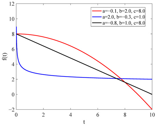
Figure 1.
Battery capacity degradation function.
2.1.2. Aggregate Warranty Replacement Demand
The identification of the battery replacement point is a crucial element in forecasting the demand for EV battery replacements. Assume a single EV is sold at time . By time T, the battery capacity degrades to G. Thus, T is the battery replacement point, which can be determined using the battery capacity degradation function
Let denote the random number of cumulative sales of EVs over the time interval . Assume that follows a homogeneous Poisson process (HPP) with a sales rate , an assumption commonly used for slow-moving sales of capital-intensive products. Since the manufacturer will eventually discontinue this product at the end of its life cycle, the HPP is truncated at time L, with the mean function given by
The HPP sales assumption is relatively reasonable, especially when the magnitude of sales volume is large and the sales curves do not exhibit obvious patterns. As illustrated in Figure 2, the sales data of Tesla Model Y in the US (Tesla Model Y US sales data. https://www.goodcarbadcar.net/tesla-model-y-sales-figures/ (accessed on 1 June 2025)) exhibits fluctuations over time. However, no discernible patterns are evident in the sales curve. In such a case, it is quite natural to assume that new-product demand arrivals follow an HPP. To further validate this assumption, we apply the Augmented Dickey–Fuller test. (The Augmented Dickey–Fuller test is a popular method that assesses the presence of a unit root in an autoregressive model , where , p is the lag order, and is white noise. In this model, testing for a unit root is equivalent to testing , which implies that the time series is nonstationary. The test statistic is , where is the ordinary least squares estimator of and represents an estimator of the standard deviation of . If the null hypothesis is rejected at the significance level , then we are confident that the time series sample is stationary. For more details, please refer to [35] (Chap 10).) to examine the sales data and find that we can be at least 82% confident that the data are stationary. In particular, the monthly sales rate is estimated as 32,996. Thus, it is reasonable and “safe” to adopt the HPP sales assumption for our analysis.
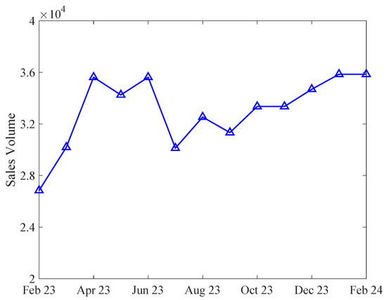
Figure 2.
Tesla Model Y US sales data.
Assume that every battery reaching the degradation threshold will be replaced with a brand-new one, and, compared to the long-term nature of the warranty period, the battery replacement time can be neglected. Let , be the random purchase dates of the units over , and be the random battery replacement demand of the i-th sold unit up to time t. Then, can be expressed as
Let be the AWRD in . By combining the sales process model and the battery replacement demand model for the -th sold unit (, can be formulated as
Note that, according to the definition of , the AWRD over any given time interval is simply the difference between the values of at the start and end points of the interval. Mathematically, this can be expressed as
Because the manufacturer is financially responsible for repairs during the warranty period, estimating the expected battery replacement demand of the sold EVs over time (AWRD) becomes one of the most important tasks. As an illustrative example, Figure 3 presents the idea of our AWRD counting procedure. One can see that all the under-warranty replacements of sold units can be aggregated at the bottom of the figure, which contribute to the AWRD (i.e., the source of battery demand).
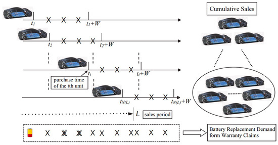
Figure 3.
Battery replacement demand generated from sold units.
Below, we will focus on deriving explicit expressions for and . Due to the limit of the sales period and the warranty period, the behavior of warranty demand varies across different periods. The following two theorems provide the expected value and variance of the AWRD up to time t.
Theorem 1.
Suppose the sales process of EVs follows an HPP and the battery replacement point is a constant T; the expected AWRD is
Proof.
Under the constant battery replacement point assumption, by time , the expected CWRD generated from all under-warranty units can be expressed as
When , it indicates that the manufacturer is fully responsible for all replacements during this period as every sold unit is still under warranty. For the subsequent interval , the warranty for some units starts to expire, a factor that is explicitly taken into account. When , the notation L in the formula is used to conclude the sales process, ensuring that only warranty replacements arising from sales within are considered. Ultimately, by the time , all units are out of warranty, and the AWRD stabilizes, remaining constant thereafter. Therefore, to derive , the time horizon needs to be divided into three distinct intervals: (1) , (2) , and (3) . The following proofs are discussed case by case due to the specific nature of in each sub-interval.
- Sub-Interval I: .
During this time period, the manufacturer has to prepare the spare batteries for all replacements of the sold EVs. By denoting , , and , we have
It is known that
Thus, we have
Sub-Interval II: .
The AWRD within this interval is different from that of sub-interval I. Especially, the sales from and should be distinguished. According to the length of the warranty, the warranties for all the units sold during will expire by time t (one can see that, even if the last unit is sold at time , its warranty expires by ). Therefore, we need to count the total number of replacements generated by each unit sold within this time period. Then, the expected AWRD of these units is written as
On the other hand, for the units sold during , their services have not expired by time t. Based on the memory-less property of the inter-arrival times and the result given in Case I, the expected CWRD of the units sold in this interval can be expressed as
Summing these two sources of AWRD yields
(11) and (14) show that
which implies that is continuous at .
- Sub-Interval III: .
Unlike sub-interval II, the sales process in this case should be truncated at L. It is clear that no sales occur beyond this period, and the cumulative number of sales is (instead of ). It is worth mentioning that some of the units sold may still be under the warranty coverage. Considering the sales before , and those units sold in the time interval , by following the similar derivations used in sub-interval II, the expected AWRD can be expressed as the sum of the following two terms.
which is obtained as
Again, (14) and (17) indicate that
which shows the continuity at . □
Another crucial issue that demands our attention is the variability or risk associated with predicting the AWRD for the manufacturer. For instance, there exists the possibility of underestimating or overestimating the demand. In an inventory system, such miscalculations can lead to substantial backorder costs or holding costs. When formulating inventory-related strategies, for a risk-averse warranty manager, merely presenting the expected AWRD is often inadequate. Additional information regarding the higher-order moments, such as the variance, of the AWRD is indispensable for controlling the risk of underestimating the warranty replacement demand. Generally, the primary challenge in deriving the variance lies in the complexity of the distribution of . Obtaining this distribution is extremely difficult, if not altogether impossible. Fortunately, having knowledge of the AWRD distribution is not a prerequisite. The following theorem presents an analytical result for the variance of the AWRD.
Theorem 2.
Assuming the product has the same sales process and replacement point as that in Theorem 1, the variance of the AWRD during is
Proof.
Given that the probability distribution of the AWRD remains unknown, we adopt an alternative methodology to investigate its variance. Initially, it is essential to ascertain the variance of the warranty replacement demand for the i-th sold unit by time t (where ). Considering that the battery replacement point for an individual unit is fixed, the variance of the warranty replacement demand for the i-th sold unit is . Consequently, the variance is solely attributable to the variability inherent in the stochastic sales process. Analogous to the approach used for determining the expectation of the AWRD, the variance should be examined across three distinct sub-intervals, with each case being discussed individually as outlined below.
- Sub-Interval I: .
Recall that all the units sold before time W are under warranty. In this sub-interval, applying (8), the variance of the AWRD is formulated as
The first term of (20) can be operated as
For the second term of (20), one has to use the definition of conditional variance one more time. Basically, given , the variance can be unfolded as
At this time, is fixed, so
and
Thus, one has
Hence, the variance of the CWRD within this sub-interval is obtained as
Sub-Interval II: .
For this time interval, it is necessary to further divide it into two sub-intervals: and . We must then analyze the events occurring within these sub-intervals separately. This is due to the fact that the warranty for units sold within the interval will have expired by time t, whereas the units sold in the interval are still under warranty. Therefore, we have
Since the Poisson process has statistically independent increments in disjoint intervals (subdomains) and , the covariance is zero. Following the similar derivations in sub-interval I, the variances in the two subdomains are
and
Therefore, the result turns out to be
(26) and (30) show that
which implies that is continuous at .
- Sub-Interval III: .
Again, the interval can be divided into and (the sales of this product will be ceased by time L). Similarly, the variance of the AWRD is
the first term is just the same as that of sub-interval II, and the other one is
then, their sum yields
(30) and (34) show that
which implies that is continuous at . □
Up to this point, we have demonstrated that both the expectation and variance of the AWRD are continuous functions with respect to time t. Nonetheless, due to their piecewise continuous nature, further exploration is required. The subsequent proposition elucidates their properties.
Proposition 1.
The mean and variance of the AWRD are both first-order differentiable and exhibit an monotonically increasing trend over the interval .
Proof.
By calculating the first-order derivatives of the expected AWRD, we obtain
Equation (36) illustrates the monotonically increasing nature of the expected value of the random variable over the considered time horizon . Similarly, the variance can be shown to possess the same property using analogous methods. □
According to Proposition 1, the first-order derivative of the mean of the AWRD can be regarded as the instantaneous demand rate. This form of demand rate is widely applied in the basic formulations for developing inventory strategies and holds significant practical value. This concept will be elaborated on in detail in the following section.
2.2. Battery Inventory Strategies for Warranty Service
Based on the AWRD forecasting model proposed in the previous section, this section develops two distinct inventory models to optimize the manufacturer’s total warranty service costs. Additionally, a comprehensive comparative analysis is conducted to evaluate the optimization performance and practical applicability of these models under identical cost parameters, providing valuable insights for managerial decision-making. Moreover, recognizing the significant divergence in demand characteristics among the three phases, , and , we employ separate inventory models for each phase using consistent methodological frameworks. Given the stochastic and time-varying demand in each phase, there is a need for a finite-horizon multi-period inventory model. This model is designed to precisely determine the optimal number of orders, reorder points, and order quantities for each time interval.
Before delving into two specific inventory models, we begin by outlining some foundational assumptions and notations essential for our discussion. To effectively frame the optimization problem, we introduce the necessary notations in Table 2. Furthermore, we establish the following assumptions to guide our analysis:
- Lead time is assumed to be zero.
- Shortages are allowed, with an associated penalty applied.
- The replenishment rate is considered infinite, resulting in instantaneous replenishment.
- The initial inventory level is set to zero.
The explanations for the reasonableness of assumptions a and c are as follows. The battery replacement discussed in this study is not an emergency repair (such as in the case of ICE vehicle failures) or real-time scheduling (such as routine production) but rather planned maintenance based on long-term degradation prediction. Specifically, the battery replenishment processes (even accounting for transportation and logistics) are typically measured in days or weeks, but the battery capacity typically requires several years to degrade from 100% to 70–80% of its initial capacity. Thus, the impact of replenishment delays on long-term inventory strategy is minimal, making the actual replenishment time negligible compared to the battery degradation cycle.
Table 2.
Notations for inventory models.
Table 2.
Notations for inventory models.
| Scripts | |
|---|---|
| k | Superscript denotes two inventory models |
| i | Subscript denotes three time phases |
| j | Subscript denotes time intervals of each phase |
| Decision Variables | |
| Total orders for Model k in phase i | |
| Order points of Model k in phase i, time interval j | |
| Shortage points for Model k in phase i, time interval j | |
| Order quantity of Model k in phase i, time interval j | |
| Parameters | |
| Time horizon of phase i | |
| K | Fixed cost of replenishment per order |
| h | Inventory holding cost per unit per unit time |
| s | Shortage cost per unit per unit time |
| Demand rate at time t for Model B, , | |
| Demand at time t in phase i, time interval j | |
| Total inventory cost of Model k in phase i | |
2.2.1. Service-Level Symmetry Model (SLSM)
In practice, managers establish inventory strategies for specific periods based on expected AWRD. However, due to sales uncertainty, there is a risk that inventory may run out before meeting all warranty claims, potentially damaging customer relations—a critical issue for new products. To mitigate this, the variance from Theorem 2 can characterize demand variability over time, facilitating the development of a conservative inventory strategy. Let denote the battery inventory reserved for warranty claims within , and the probability that the inventory is never depleted by time t. The connection between AWRD and battery inventory can thus be established as follows:
Determining necessitates knowledge of the AWRD distribution, which is challenging to acquire. Nonetheless, for sufficiently large AWRD values up to time t, this challenge can be circumvented. By approximating the AWRD distribution with a normal distribution characterized by an expectation of and a variance of , the complexity is reduced. Utilizing to denote the cumulative distribution function of the standard normal distribution , we have
Then, the battery inventory can be approximated as
The manager may choose the value of to meet the desired service level target. Specifically, this ensures that the probability of the battery inventory being sufficient to cover all warranty claims up to time t is .
In practice, for a time interval such as , the initial inventory should be . That is, the order-up-to level for the time interval is . Next, we will construct the inventory model to determine the associated replenishment strategies, specifically the number of orders, reorder points, and order-up-to levels of each time interval.
As depicted in Figure 4, we define and as the reorder point and shortage point, respectively. The inventory holding cost and shortage cost are denoted by h and s, respectively, per unit per unit time. The fixed cost of replenishment per order is K. Given a specified number of orders , a uniform time interval is applied for each replenishment cycle. Let represent the total time horizon considered. Consequently, the time interval T can be expressed as . As mentioned before, the order-up-to level for the j-th time interval during period i should be calculated as .
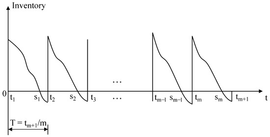
Figure 4.
SLSM: service-oriented inventory strategy with uniform time intervals.
The objective of this inventory problem is to determine the number of orders in order to keep the total cost (denoted as ) as low as possible. Denote as the demand at time t in phase i, time interval j. Then, the associated optimization problem for the i-th phase is given by
where is the upper limit of the number of orders for a time phase.
To ensure the precision and reliability of total cost evaluations, we generate warranty replacement demands via simulation experiments, with further details provided in Appendix A. Based on the Poisson sales process and the deterministic battery degradation under performance guarantee conditions, we randomly generate the AWRD at any given time point, which is considered as the actual demand , to calculate the total cost. Subsequently, given and the corresponding order-up-to level for each phase, we can calculate the shortage point (if it exists) based on the inventory consumption, thereby obtaining the actual total inventory-related cost. By iterating over , the replenishment strategy corresponding to the minimum total cost is identified as the optimal inventory strategy.
2.2.2. Cost-Efficiency Symmetry Model (CESM)
The aforementioned model represents a conservative inventory strategy that employs uniform time intervals for ordering and ensures a high level of service. However, manufacturers may sometimes opt for a strategy that generates lower inventory costs. There are two key approaches to achieving lower inventory costs. First, manufacturers can tolerate a higher volume of shortages. This is especially viable when delivery delays are not expected to dampen consumer interest. Second, adopting variable replenishment intervals has the potential to yield even greater cost savings. The CESM will delve into these aspects comprehensively.
We utilize and extend the model proposed by Teng et al. [36] to accommodate our unique three-phase demand characteristic. As illustrated in Figure 5, the cost and order parameters are consistent with those in the SLSM. The primary distinctions lie in the allowance for shortages within each time interval, encompassing both the beginning and end of the planning horizon. Additionally, we introduce variability in the time intervals. It is important to note that the demand rate is explicitly modeled as a linear function, expressed as . Assuming deterministic demand, this standard form can be obtained from the first-order calculation of the expected AWRD, as derived in Theorem 1, with respect to time t.
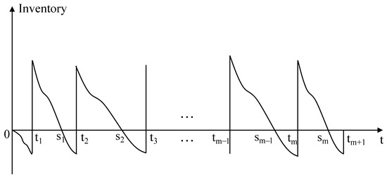
Figure 5.
CESM: flexible inventory strategy for reduced inventory costs.
Unlike the SLSM, which optimizes only the number of orders, the CESM optimizes three sets of variable parameters, namely the number of orders, order points, and shortage points, individually. Based on the derivation results from Dave, the associated optimization problem for the i-th phase is given by
where , , and are the upper limits of the number of orders, order points, and shortage points for a time phase.
The complexity of this problem stems from the integral value of m. According to the detailed derivation process of Teng et al., the following two-stage optimization method is proposed:
- (i)
- For a fixed value of , determine the optimal order points and shortage points recursively.
- (ii)
- Find the optimal total orders , which minimizes total costs over .
For the first stage, for i-th phase, to simplify the calculation, denote , and let us define by
As a result, the optimal order points are
And the optimal shortage points are
The order quantity for the time interval can be determined by calculating the cumulative demand from to .
Therefore, we need only to find to obtain and the remaining . For any chosen , if , then is chosen correctly. Teng et al. [36] solved this problem by setting a particular initial value of to accelerate the searching process of the optimal solution. However, we found that, for any given initial value within the considered time horizon, the optimal solution could be obtained both accurately and efficiently.
For the second stage, notice that is convex in (the proof is completed by Teng et al.), so the search for is reduced to finding a local minimum.
The optimization method mentioned above is applicable to both increasing and decreasing demand rates; that is, , where . However, when (i.e., a constant demand rate in phase II of our problem), the solving method of stage 1 is not applicable. Since a constant demand rate represents a simpler form of demand, we find that equal-interval replenishment is the optimal strategy. In this case, determining the first-order point is sufficient to obtain all subsequent order points, thereby establishing the complete optimal inventory policy.
Under the CESM, we also employ the methodology of the SLSM to generate warranty replacement demands and calculate the actual total inventory cost using the cost function of Model 1. This approach not only allows us to obtain the precise total inventory cost under the optimal inventory strategy derived from the CESM but also enables a more accurate assessment of the improvement capabilities of the CESM. In summary, we have successfully identified an inventory strategy suitable for three distinct phases of demand rate. Table 3 provides a detailed comparison of the SLSM and the CESM.
Table 3.
Methodological comparison between SLSM and CESM.
Moreover, the optimal strategy from the CESM can be used to enhance the strategy in the SLSM: By substituting the uniform time intervals with the variable replenishment intervals from the CESM, we can achieve a lower total cost while still maintaining the promised service level. This will also be illustrated in the numerical experiments.
3. Results
In this section, we first validate the applicability of the proposed degradation function using actual battery degradation data from leading manufacturers, and the accuracy of the derived AWRD forecasting model via simulation experiments, demonstrating their reliability and applicability across multiple datasets. Subsequently, based on the discussion of inventory models in the previous section, we compare the applicability and performance of the SLSM and the CESM under the same set of parameters, highlighting their respective strengths and weaknesses. Finally, we analyze the impact of key parameters (e.g., performance guarantee G, inventory holding cost h, and shortage cost s) on optimal decision-making.
3.1. Validation of Degradation Function and AWRD Forecasting Model
To validate the applicability of the proposed battery capacity degradation function in capturing the degradation patterns of EV batteries in real-world scenarios, we leverage real-world battery degradation data from Tesla (Model S and Model X) and a collaborating EV manufacturer. To preserve confidentiality, the manufacturer-provided datasets—collected under three distinct operating conditions—are anonymized as M1, M2, and M3 throughout this study. The original datasets, which mainly document the variation in battery capacity retention with respect to the distance covered or the charging cycle times, are transformed to a temporal scale. This is because the distance traveled and the cycle times are directly related to the driving time. Subsequently, we use the scaled data to fit the degradation curve according to the function .
As depicted in Figure 6, the fitted curves closely follow the scatter plot of the actual data points, indicating a strong correlation between the model’s predictions and the observed battery performance. Table 4 shows the detailed performance of the degradation model. Taking Figure 6a as an example, the fitted parameters (, , and ) demonstrate the model’s high accuracy, with an of 0.9892 and RMSE of 0.0030. The value of 0.9892 (close to 1) indicates that 98.92% of the capacity retention variability is captured, while the low RMSE reflects minimal prediction error.
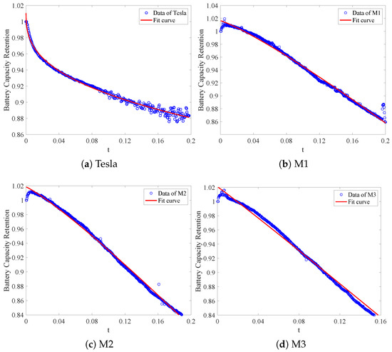
Figure 6.
Comparative analysis of battery capacity retention data and fitted curves.
Table 4.
Fitting results and performance metrics.
Figure 7 displays the battery replacement demand over a 12-year span, sampled at 0.2-year intervals, exhibiting a clear symmetrical pattern. The demand gradually increases from year 0 to year 4. This pattern is attributed to the increasing cumulative sales, with all new sales being covered by the warranty up to year 4. From year 4 to year 8, while some units become out of warranty, new sales continue to enter the market with warranty coverage. The demand plateaus and maintains a relatively stable high level during this period. After this peak, the demand symmetrically decreases from year 8 to year 12, mirroring the initial rise. This occurs as the manufacturer ceases product sales from year 8, and the warranties on existing units gradually expire until all units are out of warranty.
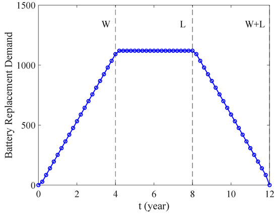
Figure 7.
Battery replacement demand (with intervals of 0.2 years): = 1000, W = 4, and L = 8.
Assuming a sales rate denoted by units per year, and a battery performance guarantee set within the range , we define the warranty period as years and the sales period as years. Battery capacity degradation is characterized by the function , as previously discussed. Subsequently, we implement Monte Carlo simulation to validate the accuracy of the AWRD forecasting model.
The inputs of the simulation include sales rate , parameters of the degradation function , warranty period W, sales period L, and the performance guarantee G. As illustrated in Figure 8, for each simulation run, we first generate all the purchase dates according to . For each purchased product during , we then generate the associated battery replacement demand based on the degradation function, from which the replacement points can be obtained. Finally, counting the total number of replacement claims during yields the simulated AWRD increments over the warranty life cycle. We conduct 1000 simulation runs for each parameter combination and calculate the mean and variance to ensure high simulation accuracy. The total warranty replacement demand during any given time interval can be obtained from the formula . Please see Appendix A for the details of the simulation algorithm.
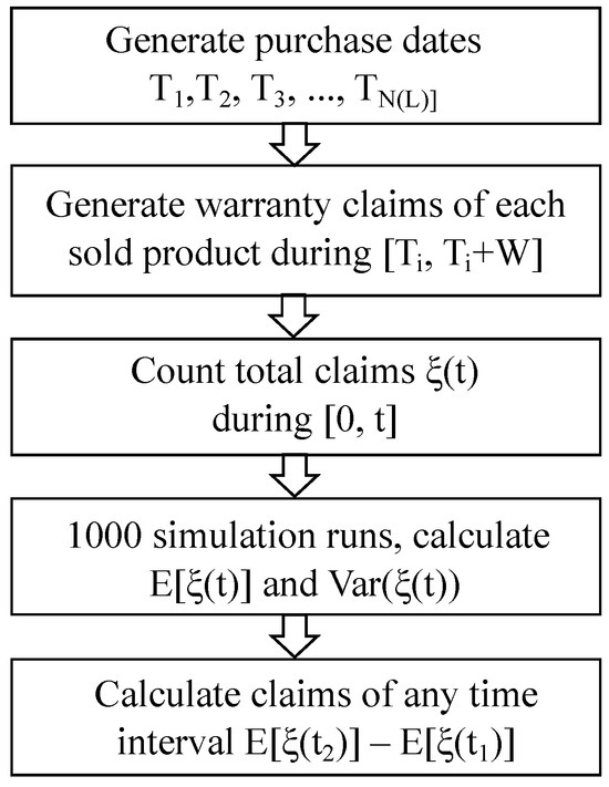
Figure 8.
Flow chart for the simulation procedure.
Figure 9 presents a comparison between the simulated and model-calculated AWRD for a performance guarantee . It is evident that the outcomes from our derived forecasting model closely align with the true quantities obtained via simulation. The simulation process was conducted 1000 times to ensure the stability and reliability of the results. Figure 10 illustrates the absolute deviation between the model calculations and the simulation. The deviation is minimal; for instance, during the considered time horizon (i.e., 12 years), the absolute deviation of the AWRD between the model and simulation is less than 20 units, which corresponds to approximately of the expected AWRD. Consequently, the AWRD forecasting model accurately captures the actual warranty replacement demand. This validation paves the way for utilizing the model to further analyze inventory strategies and conduct a detailed analysis of key parameters.
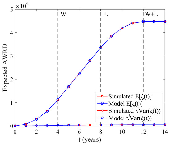
Figure 9.
Simulation and model calculation of AWRD: = 1000, W = 4, L = 8, and Sim = 1000.
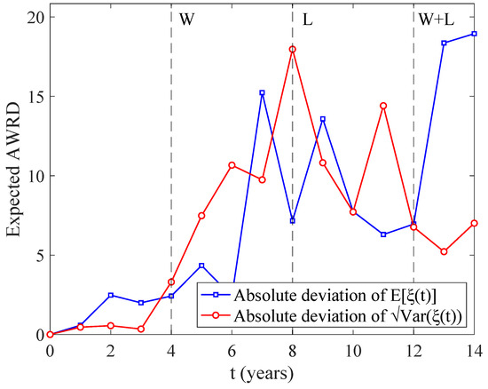
Figure 10.
Absolute deviation of simulation and model calculation: = 1000, W = 4, L = 8, and Sim = 1000.
Figure 11 illustrates the graphical trend of the AWRD across varying performance guarantee values ranging from 0.8 to 0.9. As the performance guarantee becomes more stringent, i.e., as the value of G increases, tends to rise due to a higher frequency of warranty claims. Notably, the expected AWRD increases more sharply when G is raised from 0.85 to 0.9. This phenomenon is driven by the battery capacity degradation function, which indicates a faster rate of degradation in the early stages, thereby leading to a higher incidence of warranty claims.
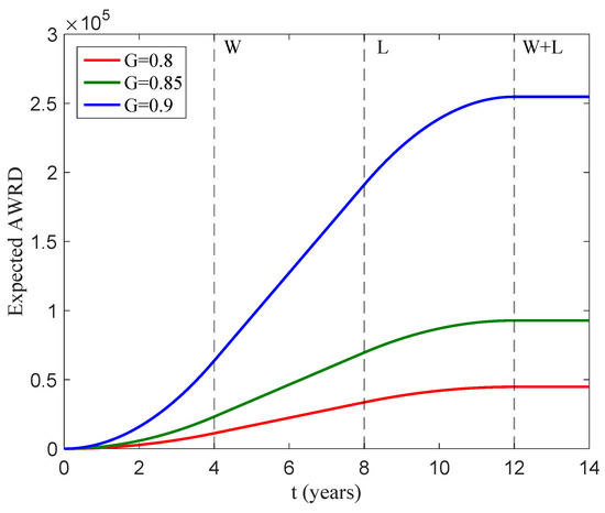
Figure 11.
Expected AWRD based on various performance guarantees: = 1000, W = 4, and L = 8.
3.2. Inventory Strategies
In this subsection, we conduct numerical experiments designed to showcase the effectiveness of our proposed inventory models. These models are tailored for an EV manufacturer that implements a performance-guaranteed warranty policy for its customers. As previously discussed, we use the degradation function derived from fitting the official data of Tesla, which is expressed as . The settings and sources of other parameters are detailed in Table 5. It should be noted that, to improve visual clarity and effectively illustrate the numerical case of our inventory model, the sales data and the time frame under consideration have been scaled to a quarter () of their original size.
Table 5.
Parameter settings.
Figure 12 presents the optimal ordering policies for the SLSM and the CESM (see detailed data in Appendix B). For each model, the optimal order quantities in Phase I exhibit an increasing trend. This is attributed to the fact that the AWRD rises as the sales volume increases. Conversely, the order quantities in Phase III decrease because the manufacturer terminates the sales process and the product gradually exceeds the warranty period. In Phase II, both models display similar trends, characterized by nearly stable ordering intervals and order quantities. This is because the demand rate remains constant during this period. The minor fluctuations in the order quantities of the SLSM during Phase II are caused by variance. Moreover, the optimal order quantities and the number of orders in Phase II remain high, which is also consistent with the trend of AWRD. Given that Phase II has the highest demand rate, manufacturers should prepare ample repair resources to meet the market demands during this period.
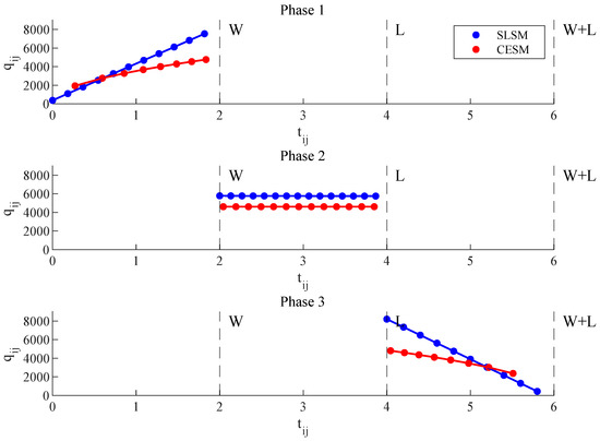
Figure 12.
Optimal ordering policies for SLSM and CESM.
Comparing the SLSM and the CESM, it can be observed that the CESM has lower optimal ordering frequencies and total costs in each phase than the SLSM, with cost reduction ratios of , , and , respectively (refer to Table 6 for a detailed comparison). This is because the CESM allows varied order intervals and permits more shortages, including shortages before the first order, to reduce costs. From Figure 9, it can be observed that the CESM’s ordering intervals in Phase 1 are gradually decreasing, with the first-order point occurring later than that of the SLSM. Conversely, in Phase 3, the ordering intervals are increasing, leading to the final order point being earlier than the SLSM’s. This is due to the lower demand rates observed in the early stages of Phase 1 and the later stages of Phase 3. Reducing the frequency of orders during these periods is beneficial for cost reduction. Note that the reduction ratio in Phase II is relatively lower than that in the other two phases. This is reasonable as the optimal strategy in this phase is to order at equal intervals, and thus the main difference between the two models in Phase II lies only in the order quantities.
Table 6.
Performance comparison of SLSM, CESM, and optimized SLSM.
From the above analysis, it is evident that the CESM has a significant advantage in cost savings. However, the SLSM is necessary when customer satisfaction is a priority. Nevertheless, we can consider further optimizing the SLSM by adopting the ordering intervals of the CESM while ensuring the service level. Such ordering intervals are more in line with the trend of warranty replacement demand changes, especially when the ordering cost is high. By reasonably reducing the ordering frequency, the total cost can be lowered. Table 6 demonstrates the effect of the enhanced optimization strategies for the SLSM. As indicated in Figure 13, the optimized ordering strategy reduces the total cost effectively, by , , and , respectively.
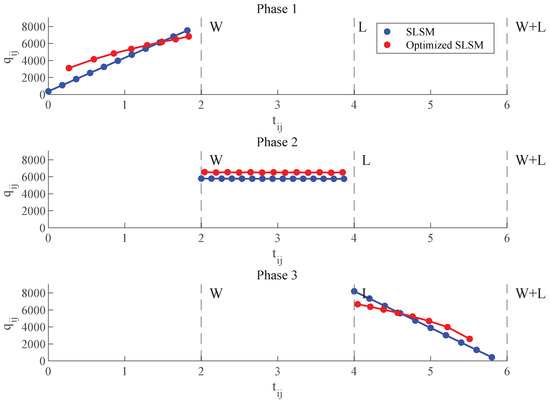
Figure 13.
Enhanced optimization strategies for SLSM.
3.3. Sensitivity Analysis
In this subsection, we aim to investigate the impacts of key parameters on optimal solutions, focusing on three distinct categories: inventory-related cost parameters (), the battery capacity degradation function (), and warranty-related parameters (). Given that the SLSM and the CESM share a similar cost structure, we will use the CESM as an example to analyze the impact of these parameters. In each sensitivity analysis, we vary a single parameter while keeping all the other parameters fixed. All the parameter values remain consistent with those presented in Table 6.
Figure 14, Figure 15 and Figure 16 illustrate the trends of optimal ordering policies based on different cost parameters. It can be observed that the optimal total cost increases with the rise in fixed-order cost, inventory holding cost, and shortage cost. This trend is reasonable as an increase in any of these costs will lead to a higher total cost. Additionally, the number of orders shows different trends with the increase in these three cost parameters: it decreases with the fixed-order cost and increases with both the inventory holding cost and the shortage cost. This is reasonable. When the cost of placing an order is high, manufacturers tend to reduce the order quantity to lower the associated ordering costs. Conversely, when the inventory holding cost or shortage cost is high, more frequent orders are needed to reduce the average inventory level and to meet demand, thereby preventing significant shortages. Moreover, it is evident that the total cost in Phase 2 is consistently much higher than that in the other two phases, while the costs in Phase 1 and Phase 3 are almost equal. This is because the three phases are of equal duration, and Phase 2 has the highest demand rate, resulting in the highest total cost. In contrast, the demand rates in Phase 1 and Phase 3 increase and decrease, respectively, leading to similar total costs.
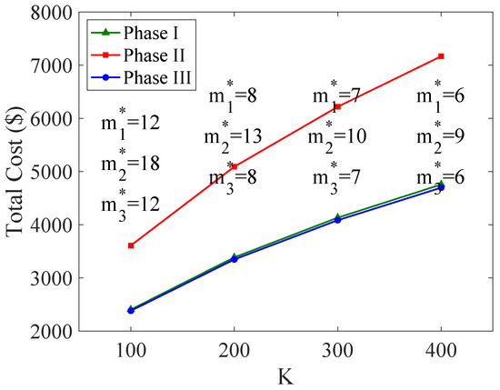
Figure 14.
Optimal total inventory cost varies with K.
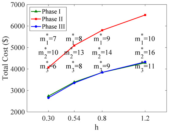
Figure 15.
Optimal total inventory cost varies with h.
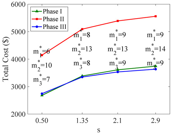
Figure 16.
Optimal total inventory cost varies with s.
Table 7 presents the optimal inventory strategies for different degradation functions. Combined with Figure 6, it can be observed that the degradation rate of Tesla’s batteries shows a decreasing trend and is lower than that of M1, M2, and M3 in the later stages. When , Tesla has a lower replacement demand, resulting in the lowest total cost. In contrast, the degradation functions of M1, M2, and M3 exhibit an increasing trend in degradation rates, which consequently leads to a similar increasing trend in total costs. In summary, the characteristics of battery degradation have a significant impact on battery warranty inventory management. Therefore, accurately characterizing the degradation trend of batteries and strengthening research and analysis related to battery degradation can help to further improve the current status of warranty part inventory management.
Table 7.
Optimal inventory strategies for different degradation functions.
Table 8 shows that both the optimal total cost and the number of orders exhibit accelerated growth as the performance guarantee G increases. This phenomenon can be attributed to the non-linear nature of battery degradation, which occurs at a gradually decreasing rate. Consequently, when G is set at a higher level, individual products generate warranty demands more frequently, leading to a sharp increase in total demand. Therefore, manufacturers should weigh the relationship between the performance guarantee level and the related costs. For instance, in this numerical experiment, keeping the value of G within the range of 0.8 to 0.85 can ensure reasonable customer satisfaction while avoiding a sharp increase in costs.
Table 8.
Optimal inventory strategies for different warranty-related parameters.
When the warranty period W increases from 1.0 to 2.0, both Phase 1 and Phase 3 will be prolonged (with an increase in costs), while Phase 2 will be shortened (with a decrease in costs). However, since the total consideration period is extended, the total cost of the three stages shows an increasing trend. The warranty period is usually fixed (for example, by benchmarking similar products in the market or referring to relevant policy regulations), but manufacturers can also consider appropriately adjusting the warranty period to effectively manage warranty costs. Finally, the impact of the sales rate on the optimal inventory strategy is quite intuitive: the larger the , the greater the warranty demand and the total cost, but this is also accompanied by more sales profit, which is a sign of positive development.
4. Discussion
4.1. Concluding Remarks
This study aims to address a comprehensive battery warranty demand forecasting and inventory strategy optimization problem throughout the entire warranty period from a manufacturer’s perspective. By coupling stochastic EV sales dynamics with battery performance degradation thresholds, we derive the closed-form solution for the mean and variance of the aggregate warranty replacement demand (AWRD). Subsequently, two inventory optimization models are proposed: the Service-Level Symmetry Model (SLSM), which prioritizes reliability and customer satisfaction, and the Cost-Efficiency Symmetry Model (CESM), which focuses on economic balance and inventory cost minimization. The main findings of this work are summarized as follows.
- (i)
- To mathematically characterize the degradation trends of EV batteries, we employ a function capable of accurately capturing the inherent non-linear characteristics of battery degradation, such as decreasing decay rates over time. Additionally, the function demonstrates flexibility in fitting diverse degradation patterns, reflecting its adaptability and broad generalizability in modeling various degradation processes. The function’s practical utility was rigorously validated using actual battery degradation data from leading manufacturers, ensuring its relevance and reliability in real-world applications.
- (ii)
- Given the predetermined threshold of battery performance, which corresponds to the performance guarantee specified in the warranty policy provided by EV manufacturers to consumers, we establish a framework to determine individual EV battery replacement cycles by integrating this performance guarantee with our battery capacity degradation function. Subsequently, by incorporating stochastic sales processes into our analytical model, we derive both the mean and variance of AWRD at any given time point. This theoretical framework provides a robust foundation for optimizing operational activities at service centers, particularly in terms of inventory management and resource allocation.
- (iii)
- Based on distinct assumptions regarding service levels and ordering intervals, we develop two inventory models that are specifically adapted to our demand forecasting framework through normal approximation and demand rate computation. The comparative analysis demonstrates that the CESM achieves superior cost performance, reducing the total cost by 20.3% while maintaining operational stability. Furthermore, incorporating CESM-derived strategies into the SLSM yields a hybrid solution that preserves service-level guarantees and achieves a 3.9% cost reduction. This optimization approach provides valuable insights for inventory management system design and operational decision-making.
4.2. Limitations and Future Work
First, real-world warranty policies typically incorporate not only warranty periods but also mileage limitations. Thus, investigating two-dimensional performance-guaranteed warranty policies that simultaneously consider both time and mileage factors represents a promising direction for future research. Second, while incorporating the stochastic nature of battery degradation would inevitably increase model complexity, such an enhancement would significantly improve the model’s alignment with real-world scenarios, thereby enhancing its practical applicability and predictive accuracy. Finally, this work is initially based on the stable sales assumption (HPP); future research could generalize the method to adapt to nonstationary sales scenarios, expanding its practical applicability.
Author Contributions
M.F.: Conceptualization, Methodology, Software, Writing, Validation, Visualization. W.X.: Conceptualization, Methodology, Validation, Project Administration, Funding Acquisition. X.W.: Validation, Writing, Visualization, Funding Acquisition. All authors have read and agreed to the published version of the manuscript.
Funding
This research was funded by National Natural Science Foundation of China (#71971085).
Data Availability Statement
The original contributions presented in this study are included in the article. Further inquiries can be directed to the corresponding author.
Acknowledgments
The authors would like to sincerely thank the editor and reviewers for their kind comments.
Conflicts of Interest
The authors declare no conflicts of interest.
Appendix A. Simulation Algorithm for Forecasting AWRD
| Algorithm A1 Simulation Algorithm for Forecasting AWRD |
| Input: W, L, , , t, Output: Mean and variance of AWRD: ,
|
Appendix B. Optimal Ordering Policies
Table A1.
Optimal ordering policies of SLSM.
Table A1.
Optimal ordering policies of SLSM.
| Order No. | Phase 1 | Phase 2 | Phase 3 | |||
|---|---|---|---|---|---|---|
| 1 | 0.000 | 373 | 2.000 | 5785 | 4.000 | 8202 |
| 2 | 0.182 | 1097 | 2.133 | 5780 | 4.200 | 7342 |
| 3 | 0.364 | 1816 | 2.267 | 5776 | 4.400 | 6480 |
| 4 | 0.546 | 2533 | 2.400 | 5773 | 4.600 | 5618 |
| 5 | 0.727 | 3250 | 2.533 | 5770 | 4.800 | 4755 |
| 6 | 0.909 | 3965 | 2.667 | 5768 | 5.000 | 3892 |
| 7 | 1.091 | 4680 | 2.800 | 5766 | 5.200 | 3028 |
| 8 | 1.273 | 5394 | 2.933 | 5764 | 5.400 | 2164 |
| 9 | 1.455 | 6109 | 3.067 | 5762 | 5.600 | 1299 |
| 10 | 1.636 | 6822 | 3.200 | 5761 | 5.800 | 433 |
| 11 | 1.818 | 7536 | 3.333 | 5759 | 6.000 | – |
| 12 | 2.000 | – | 3.467 | 5758 | ||
| 13 | 3.600 | 5757 | ||||
| 14 | 3.733 | 5756 | ||||
| 15 | 3.867 | 5755 | ||||
| 16 | 4.000 | – | ||||
| m* | 11 | 15 | 10 | |||
| TC* | 4434.03 | 6136.52 | 4271.40 | |||
Table A2.
Optimal ordering policies of CESM.
Table A2.
Optimal ordering policies of CESM.
| Order No. | Phase 1 | Phase 2 | Phase 3 | |||
|---|---|---|---|---|---|---|
| 1 | 0.269 | 1935 | 2.043 | 4615 | 4.045 | 4803 |
| 2 | 0.596 | 2756 | 2.194 | 4615 | 4.211 | 4594 |
| 3 | 0.857 | 3278 | 2.344 | 4615 | 4.384 | 4363 |
| 4 | 1.085 | 3676 | 2.495 | 4615 | 4.568 | 4105 |
| 5 | 1.292 | 4005 | 2.645 | 4615 | 4.764 | 3808 |
| 6 | 1.484 | 4287 | 2.796 | 4615 | 4.979 | 3456 |
| 7 | 1.665 | 4537 | 2.946 | 4615 | 5.220 | 3011 |
| 8 | 1.836 | 4760 | 3.097 | 4615 | 5.510 | 2363 |
| 9 | 2.000 | – | 3.247 | 4615 | 6.000 | – |
| 10 | 3.398 | 4615 | ||||
| 11 | 3.548 | 4615 | ||||
| 12 | 3.699 | 4615 | ||||
| 13 | 3.849 | 4615 | ||||
| 14 | 4.000 | – | ||||
| m* | 8 | 13 | 8 | |||
| TC* | 3387.40 | 5091.98 | 3348.88 | |||
Table A3.
Optimal ordering policies of optimized SLSM.
Table A3.
Optimal ordering policies of optimized SLSM.
| Order No. | Phase 1 | Phase 2 | Phase 3 | |||
|---|---|---|---|---|---|---|
| 1 | 0.269 | 3110 | 2.043 | 6549 | 4.045 | 6680 |
| 2 | 0.596 | 4147 | 2.194 | 6500 | 4.211 | 6379 |
| 3 | 0.857 | 4829 | 2.344 | 6539 | 4.384 | 6044 |
| 4 | 1.085 | 5358 | 2.495 | 6492 | 4.568 | 5669 |
| 5 | 1.292 | 5798 | 2.645 | 6532 | 4.764 | 5227 |
| 6 | 1.484 | 6195 | 2.796 | 6486 | 4.979 | 4697 |
| 7 | 1.665 | 6502 | 2.946 | 6527 | 5.220 | 3988 |
| 8 | 1.836 | 6829 | 3.097 | 6482 | 5.510 | 2595 |
| 9 | 2.000 | – | 3.247 | 6524 | 6.000 | – |
| 10 | 3.398 | 6479 | ||||
| 11 | 3.548 | 6521 | ||||
| 12 | 3.699 | 6476 | ||||
| 13 | 3.849 | 6518 | ||||
| 14 | 4.000 | – | ||||
| m* | 8 | 13 | 8 | |||
| TC* | 4193.51 | 6118.02 | 3955.26 | |||
References
- International Energy Agency. Global EV Outlook 2024; Technical Report; IEA: Paris, France, 2024. [Google Scholar]
- Kim, S.; Lee, J.; Lee, C. Does driving range of electric vehicles influence electric vehicle adoption? Sustainability 2017, 9, 1783. [Google Scholar] [CrossRef]
- Wu, J.; Liao, H.; Wang, J.W.; Chen, T. The role of environmental concern in the public acceptance of autonomous electric vehicles: A survey from China. Transp. Res. Part F Traffic Psychol. Behav. 2019, 60, 37–46. [Google Scholar] [CrossRef]
- Zhang, W.; Luo, R.; Mao, Q.; Zhu, Z. Optimal production cooperation strategies for automakers considering different sales channels under dual credit policy. Comput. Ind. Eng. 2024, 187, 109769. [Google Scholar] [CrossRef]
- Wu, F.; Sioshansi, R. A stochastic flow-capturing model to optimize the location of fast-charging stations with uncertain electric vehicle flows. Transp. Res. Part D Transp. Environ. 2017, 53, 354–376. [Google Scholar] [CrossRef]
- Huang, Y.; Kockelman, K.M. Electric vehicle charging station locations: Elastic demand, station congestion, and network equilibrium. Transp. Res. Part D Transp. Environ. 2020, 78, 102179. [Google Scholar] [CrossRef]
- Zhang, D.; Liu, Y.; He, S. Vehicle assignment and relays for one-way electric car-sharing systems. Transp. Res. Part B Methodol. 2019, 120, 125–146. [Google Scholar] [CrossRef]
- Luo, Y.; Feng, G.; Wan, S.; Zhang, S.; Li, V.; Kong, W. Charging scheduling strategy for different electric vehicles with optimization for convenience of drivers, performance of transport system and distribution network. Energy 2020, 194, 116807. [Google Scholar] [CrossRef]
- Karim, R.; Suzuki, K. Analysis of warranty claim data: A literature review. Int. J. Qual. Reliab. Manag. 2005, 22, 667–686. [Google Scholar] [CrossRef]
- Wu, S. Warranty data analysis: A review. Qual. Reliab. Eng. Int. 2012, 28, 795–805. [Google Scholar] [CrossRef]
- Wu, S. A review on coarse warranty data and analysis. Reliab. Eng. Syst. Saf. 2013, 114, 1–11. [Google Scholar] [CrossRef]
- Kleyner, A.; Sandborn, P. Forecasting the cost of unreliability for products with two-dimensional warranties. In Proceedings of the European Safety and Reliability Conference, Estoril, Portugal, 18–22 September 2006; Volume 1903, p. 1908. [Google Scholar]
- Rai, B.K. Warranty spend forecasting for subsystem failures influenced by calendar month seasonality. IEEE Trans. Reliab. 2009, 58, 649–657. [Google Scholar] [CrossRef]
- Majeske, K.D. A non-homogeneous Poisson process predictive model for automobile warranty claims. Reliab. Eng. Syst. Saf. 2007, 92, 243–251. [Google Scholar] [CrossRef]
- Wu, S.; Zuo, M.J. Linear and nonlinear preventive maintenance models. IEEE Trans. Reliab. 2010, 59, 242–249. [Google Scholar]
- Shokouhyar, S.; Ahmadi, S.; Ashrafzadeh, M. Promoting a novel method for warranty claim prediction based on social network data. Reliab. Eng. Syst. Saf. 2021, 216, 108010. [Google Scholar] [CrossRef]
- Wu, S.; Akbarov, A. Support vector regression for warranty claim forecasting. Eur. J. Oper. Res. 2011, 213, 196–204. [Google Scholar] [CrossRef]
- Chehade, A.; Savargaonkar, M.; Krivtsov, V. Conditional Gaussian mixture model for warranty claims forecasting. Reliab. Eng. Syst. Saf. 2022, 218, 108180. [Google Scholar] [CrossRef]
- Luo, M.; Wu, S. A comprehensive analysis of warranty claims and optimal policies. Eur. J. Oper. Res. 2019, 276, 144–159. [Google Scholar] [CrossRef]
- Wang, X.; Xie, W.; Ye, Z.S.; Tang, L.C. Aggregate discounted warranty cost forecasting considering the failed-but-not-reported events. Reliab. Eng. Syst. Saf. 2017, 168, 355–364. [Google Scholar] [CrossRef]
- Jin, T.; Liao, H. Spare parts inventory control considering stochastic growth of an installed base. Comput. Ind. Eng. 2009, 56, 452–460. [Google Scholar] [CrossRef]
- Hu, Q.; Boylan, J.E.; Chen, H.; Labib, A. OR in spare parts management: A review. Eur. J. Oper. Res. 2018, 266, 395–414. [Google Scholar] [CrossRef]
- Bounou, O.; El Barkany, A.; El Biyaali, A. Inventory models for spare parts management: A review. Int. J. Eng. Res. Afr. 2017, 28, 182–198. [Google Scholar] [CrossRef]
- Zhang, S.; Huang, K.; Yuan, Y. Spare parts inventory management: A literature review. Sustainability 2021, 13, 2460. [Google Scholar] [CrossRef]
- Van der Auweraer, S.; Boute, R.N.; Syntetos, A.A. Forecasting spare part demand with installed base information: A review. Int. J. Forecast. 2019, 35, 181–196. [Google Scholar] [CrossRef]
- Dendauw, P.; Goeman, T.; Claeys, D.; De Turck, K.; Fiems, D.; Bruneel, H. Condition-based critical level policy for spare parts inventory management. Comput. Ind. Eng. 2021, 157, 107369. [Google Scholar] [CrossRef]
- Turrini, L.; Meissner, J. Spare parts inventory management: New evidence from distribution fitting. Eur. J. Oper. Res. 2019, 273, 118–130. [Google Scholar] [CrossRef]
- Kim, B.; Park, S. Optimal pricing, EOL (end of life) warranty, and spare parts manufacturing strategy amid product transition. Eur. J. Oper. Res. 2008, 188, 723–745. [Google Scholar] [CrossRef]
- Panagiotidou, S. Joint optimization of spare parts ordering and maintenance policies for multiple identical items subject to silent failures. Eur. J. Oper. Res. 2014, 235, 300–314. [Google Scholar] [CrossRef]
- Yan, T.; Lei, Y.; Wang, B.; Han, T.; Si, X.; Li, N. Joint maintenance and spare parts inventory optimization for multi-unit systems considering imperfect maintenance actions. Reliab. Eng. Syst. Saf. 2020, 202, 106994. [Google Scholar] [CrossRef]
- Zhang, W.; He, S.; Zhang, X.; Zhao, X. Joint optimization of job scheduling, condition-based maintenance planning, and spare parts ordering for degrading production systems. Reliab. Eng. Syst. Saf. 2024, 252, 110447. [Google Scholar] [CrossRef]
- Zhang, J.; Zhao, X.; Song, Y.; Qiu, Q. Joint optimization of condition-based maintenance and spares inventory for a series–parallel system with two failure modes. Comput. Ind. Eng. 2022, 168, 108094. [Google Scholar] [CrossRef]
- Wang, J.; Fu, Y.; Zhou, J.; Yang, L.; Yang, Y. Condition-based maintenance for redundant systems considering spare inventory with stochastic lead time. Reliab. Eng. Syst. Saf. 2025, 257, 110837. [Google Scholar] [CrossRef]
- Xie, W.; Liu, Z.; Fu, K.; Zhong, S. Spare parts provisioning strategy of warranty repair demands for capital-intensive products. Proc. Inst. Mech. Eng. Part O J. Risk Reliab. 2024, 1748006X241272829. [Google Scholar] [CrossRef]
- Fuller, W.A. Introduction to Statistical Time Series; John Wiley & Sons: Hoboken, NJ, USA, 1995. [Google Scholar]
- Teng, J.T.; Chern, M.S.; Yang, H.L. An optimal recursive method for various inventory replenishment models with increasing demand and shortages. Nav. Res. Logist. 1997, 44, 791–806. [Google Scholar] [CrossRef]
Disclaimer/Publisher’s Note: The statements, opinions and data contained in all publications are solely those of the individual author(s) and contributor(s) and not of MDPI and/or the editor(s). MDPI and/or the editor(s) disclaim responsibility for any injury to people or property resulting from any ideas, methods, instructions or products referred to in the content. |
© 2025 by the authors. Licensee MDPI, Basel, Switzerland. This article is an open access article distributed under the terms and conditions of the Creative Commons Attribution (CC BY) license (https://creativecommons.org/licenses/by/4.0/).