A Hypergraph-Based Approach to Attribute Reduction in an Incomplete Decision System

Abstract

Attribute reduction has been demonstrated to be an effective approach for addressing fuzziness and uncertainty in data analysis, especially for data dimension reduction. As an extension of graphs, hypergraphs have been established by prior research as a potent mathematical framework for attribute reduction in decision systems. However, current studies rarely explore the integration of hypergraphs and rough set theories for attribute reduction in incomplete decision systems. To bridge this theoretical gap, this paper proposes a novel hypergraph-based attribute reduction method for incomplete decision systems through a matrix. Firstly, we introduce two types of construction methods for the characteristic matrices of a hypergraph, and the characteristic matrix decomposition relationship between them is examined. Moreover, some features in hypergraphs including transversal are systematically investigated via these characteristic matrices. Secondly, using the characteristic matrices of the hypergraphs derived from an incomplete information system, a hypergraph-based method is developed for the process of attribute reduction in incomplete information systems via a discernibility matrix. Finally, we discuss the attribute reduction method of incomplete decision systems, and establish a new judgment method for the attribute reduction in incomplete decision systems through the constructed characteristic matrices of hypergraphs.

1. Introduction

In many data mining processes, there is often a challenge of high data dimensionality. The biggest challenge of high dimensionality is that thousands of features significantly increase the complexity of data mining [1]. Therefore, dimensionality reduction methods are often used as a data preprocessing step to improve recognition accuracy. This process is known as feature selection. Feature selection based on rough set theory [2], also called attribute reduction, is to reduce redundant features to find a minimum feature subset, which provides the same classification information as the original feature set and has been successfully applied to machine learning and pattern recognition. Simultaneously, the upper and lower approximation sets, which are the core concept of classical rough sets, are used to describe positive regions. Therefore, how to reform the method of calculating approximate sets to improve the efficiency of attribute reduction has become an important research topic for scholars [3]. In fact, all calculations in the rough set models, such as feature selection and rule extraction, are almost all related to the calculation of the positive domain. Obviously, the method for calculating the approximate set is a very important research topic on rough sets.

The classical rough set theory has been proved to be effective in discovering knowledge rules from complete decision systems (CDSs). Since the classic rough set is based on the equivalence relation, this limits its wide application. In order to strengthen the performance of the classic rough sets’ algorithm, many scholars have combined rough sets with other theories and obtained some research results [4,5]. Unfortunately, the classical rough set theory is not suitable for incomplete decision systems (IDSs). However, in real life, there exist incomplete information systems (IISs) with missing values [6,7]. This also urges scholars to explore new methods of attribute reduction to meet the actual needs [8,9].

Feature-selection-based rough sets have been discussed over recent years [10,11]. For example, using similarity relations, Kryszkiewicz [12] presented a method for eliminating knowledge or attributes from an IDS and proposed a new method for calculating all optimal certain rules from IDSs. Following such work, the notion of a maximal consistent block is proposed to deal with the problem of knowledge discovery in IDSs [13]. Furthermore, a rough set-based method for knowledge acquisition in IDSs was also obtained in [14]. Based on the maximal consistent block, Qian et al. [15] also defined and proposed an extension of combinatorial entropy for the combination entropy or mutual information. Based on Kryszkiewicz’s work, Wu et al. studied attribute reduction in IDSs from the viewpoint of the Dempster–Shafer theory of evidence and presented the relationships among classical reducts, belief reducts and plausibility reducts [16]. Yang et al. proposed a neighborhood-system-based method for the incomplete information system [17]. Integrating the attribute measure based on the indiscernibility relation and discernibility relation, Shu et al. [18] developed two efficient attribute reduction algorithms for computing reductions in an IIS.

In recent years, the research on feature selection based on matrix and graph methods has attracted a lot of attention [19]. Wang et al. [20] studied the relationship between matroids and rough sets through graphs and matrices, and gave the graph representation of lower and upper approximations. In [21,22], Chen et al. studied the problem of attribute reduction in classic rough sets through the vertex cover of the graph and discussed the attribution reduction method based on graphs. Moreover, based on the hypergraph model, the attribution reduction method of the covering decision system was studied. Tan and Li studied reduction in covering decision information systems by matrix-based methods and the notions of minimal and maximal descriptions in covering decision information systems were proposed in [23]. Based on covering rough sets, Yang et al. [24] proposed a heuristic graph-based description vector algorithm for feature selection in a covering decision system. Mao et al. studied the attribute problem in a formal context by applying diagrams of hypergraphs, thus realizing the visualization of attribute reduction [25]. In addition, matrices have been used in the theoretical basis and application framework of rough sets, such as characteristic matrices [26,27] and discernibility matrices [28]. It can be seen that the technology of graphs and matrices is widely used and attracts more and more attention [29,30]. In a framework, it is very interesting and useful to study the feature selection of rough sets through graph and matrix methods. However, there are few studies to solve attribute reduction in IDSs based on matrices and graphs. This prompted us to explore the properties of IDSs from the perspective of matrices and graphs and propose a novel method for the attribute reduction of IDSs based on matrices and graphs.

In this paper, we construct the matrix representation of hypergraphs and apply them to the attribute reduction of IDSs. The main contributions of this study are summarized as follows: (1) Two types of characteristic matrices of a hypergraph and the relationship between them is proven, where one of the characteristic matrices is the transpose product of the other characteristic matrix. Through matrix operations, key features of hypergraph are systematically characterized. (2) A hypergraph-based method is established for the attribute reduction in an IIS via the discernibility matrix derived from characteristic matrices of hypergraphs. (3) A novel judgment method is given for the attribute reduction in both consistent and inconsistent IDSs using characteristic matrices of hypergraphs.

This paper is organized as follows. Section 2 reviews some basic concepts related to incomplete information systems and hypergraphs. In Section 3, the characteristic matrices of hypergraphs are constructed and some features of hypergraphs are given by matrix representation. In Section 4, the characteristics matrices of hypergraphs are employed to the attribute reduction in incomplete decision systems. A new judgment method for attribute reduction in IISs based on the constructed characteristic matrix is proposed. Section 5 concludes this paper.

2. Preliminaries

In this section, we briefly review several basic concepts, such as incomplete information systems, hypergraphs and so on.

2.1. Incomplete Information Systems

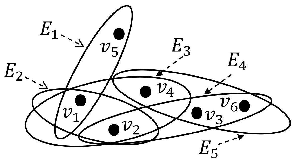
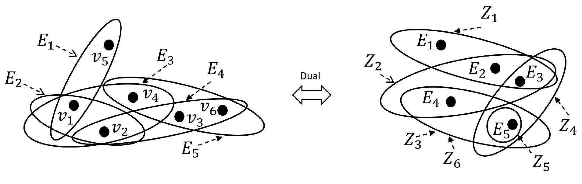
Firstly, we will introduce the concepts of information system and incomplete information system.

Definition 1

([2]). An information system (IS) is defined as a 4-tuple $\mathcal{S}=(U,AT,V,f)$, where U is a nonempty finite set of objects, i.e., the universe of discourse and $AT$ is a nonempty finite set of attributes. $V={\cup }_{a\in AT}{V}_a$, $V_a$ is a domain of the attribute a, and $f:U\times AT⟼V$ is a function such that such that $f(x,a)\in V_a$ for any $a\in AT,x\in U$.

For any subset of attributes $A\subseteq AT$, A can induce an indiscernibility relation $IND\left(A\right)$, where $IND\left(A\right)=\left\{\right(x,y)\in U\times U|\forall a\in A,f(x,a)=f(y,a)\}$. Obviously, $IND\left(A\right)$ determines an equivalence relation U, which forms a partition denoted as $U/IND\left(A\right)=\left\{{\left[x\right]}_A\right|x\in U\}$, where ${\left[x\right]}_A=\{y\in U|(x,y)\in IND\left(A\right)\}$.

In practical applications, it is common to encounter datasets that contain missing information, which hinders the ability to analyze the relationships among objects within a comprehensive framework. To solve such a situation, a null value denoted by ∗ is usually introduced to those attributes. For an information system $\mathcal{S}=(U,A,V,f)$, if $x\in U,a\in AT$ exist such that $f(x,a)=\ast$, then the information system $\mathcal{S}$ is called an incomplete information system (IIS).

For an IIS, the tolerance relation is introduced to handle incomplete information systems [6].

Definition 2

([6]). Suppose $\mathcal{S}=(U,AT,V,f)$ is an IIS. For any $A\in AT$, A determines a binary relation denoted by $SIM\left(A\right)$ defined as follows: $SIM\left(A\right)=\left\{\right(x,y)\in U\times U|\forall a\in A,f(x,a)=f(y,a)$ or $f(x,a)=\ast$ or $f(y,a)=\ast \}$.

$SIM\left(A\right)$ is called a similarity relation on U, which is reflexive and symmetric [6], and $SIM\left(A\right)={\bigcap }_{a\in A}SIM\left(\left\{a\right\}\right)$. Moreover, for any $x\in U$, the similarity class of object x is denoted as $S_A\left(x\right)=\{y\in U|(x,y)\in SIM\left(A\right)\}$. In particular, $S_{\left\{a\right\}}\left(x\right)$ is shorted as $S_a\left(x\right)$. The set of all the similarity classes of objects is denoted by $U/SIM\left(A\right)=\left\{S_A\left(x\right)\right|x\in U\}$. It is worth noting that $U/SIM\left(A\right)$ is usually not a partition on U, but a covering on U.

An IS is a decision system (DS) $(U,AT\cup \{d\},V,f)$, where $AT$ is called the conditional attribute set and d is called decision attribute, which satisfies $d\notin AT$. Then $(U,AT\cup \{d\},V,f)$ is called a complete decision information system if $f(x,a)\ne \ast$ for any $a\in AT\cup \left\{d\right\}$. Otherwise, $(U,AT\cup \{d\left\}\right)$ is called a incomplete decision system (IDS).

Definition 3

([6,31]). Suppose $(U,AT,V,f)$ is an IIS and $A\subseteq AT$. If $SIM\left(AT\right)=SIM\left(A\right)$, i.e., $S_{AT}\left(x\right)=S_A\left(x\right)$ for any $x\in U$, then A is called a consistent set of $\mathcal{S}$ and no proper subset of A is consistent, then A is called a reduct of $AT$.

For an IDS $(U,AT\cup \{d\},V,f)$ and $A\subseteq AT$, we denote ${{\rm Y}}_A\left(x\right)=\left\{f(y,d)\right|y\in S_A\left(x\right)\}$. If $\left|{\rm Y}\right(x\left)\right|=1$ for any $x\in U$, namely $S_{AT}\left(x\right)\subseteq {\left[x\right]}_d$ for any $x\in U$, then $(U,AT\cup \{d\left\}\right)$ is called a consistent IDS. Otherwise it is called an inconsistent IDS.

Based on similarity relations, one can induce the upper and lower approximations of an arbitrary subset X of U. They are defined as follows. It is worth noting that Definition 3 is actually a promotion of Pawlak’s rough set model proposed in [2].

Definition 4

([6,31]). Suppose $(U,AT,V,f)$ is an IIS and $A\subseteq AT$. For any $X\subseteq U$, the lower and upper approximations of X are defined as follows:

$$\underline{A}\left(X\right)=\{x\in U|[S_A\left(x\right)\subseteq X\},\overline{A}\left(X\right)=\{x\in U|S_A\left(x\right)\cap X\ne \varnothing \}.$$

Some properties of the lower and upper approximations of X are presented by the following proposition.

Proposition 1

([6,31]). Suppose $(U,AT,V,f)$ is an IIS and $A,B\subseteq AT$. For any $X,Y\subseteq U$, the following properties hold:

(1) 

$\underline{A}\left(X\right)=\overline{A}\left(X\right)=X$, where $X=U,\varnothing$;

(2) 

$\underline{A}\left(X\right)\subseteq X\subseteq \overline{A}\left(X\right)$;

(3) 

$\underline{A}\left(X\right)={\left(\overline{A}\left(X^C\right)\right)}^C$, where $X^C=U-X$;

(4) 

$X\subseteq Y,\underline{A}\left(X\right)\subseteq \underline{A}\left(Y\right),\overline{A}\left(X\right)\subseteq \overline{A}\left(Y\right)$;

(5) 

$\underline{A}(X\cap Y)=\underline{A}\left(X\right)\cap \underline{A}\left(Y\right)$, $\overline{A}(X\cup Y)=\overline{A}\left(X\right)\cup \overline{A}\left(Y\right)$;

(6) 

If $B\subseteq A$, then $\underline{B}\left(X\right)\subseteq \underline{A}\left(X\right)$ and $\overline{A}\left(X\right)\subseteq \overline{B}\left(X\right)$.

2.2. Hypergraphs

A hypergraph represents a generalization of graphs, which are mathematically defined by hyperedges that connect arbitrary sets of vertices. We now proceed to formally introduce its fundamental concepts and properties.

Definition 5

(Hypergraph [32]). Suppose $\mathcal{V}=\{v_1,v_2,\dots ,v_n\}$ is a finite and $\xi =\{E_1,E_2,\dots ,E_m\}$ is a set of subsets of $\mathcal{V}$. $\mathit{H}=(\mathcal{V},\xi )$ is called a hypergraph on $\mathcal{V}$ if $\mathit{H}$ satisfies that

(1) 

$E_i\ne \varnothing (1\le i\le m)$;

(2) 

${\cup }_{i=1}^m{E}_i=\mathcal{V}$.

Based on Definition 5, the elements of $\mathcal{V}$ and the elements of $\xi$ are called vertices and edges of hypergraph $\mathit{H}$. Moreover, if $E_i\subseteq E_j\Rightarrow E_i=E_j$, then hypergraph $\mathit{H}$ is called a simple hypergraph. In a hypergraph $\mathit{H}$, the set of all the hyperedges containing the vertex $v\in \mathcal{V}$ is denoted as $D_{\mathit{H}}\left(v\right)$, and the number $|D_{\mathit{H}}\left(v\right)|$ is called the degree of vertex v. For any edge $E_i\in \xi$, the number $|E_i|$ is called the degree of hyperedge. For any two vertices in $\mathcal{V}$, they are said to be incident or neighborhood each other if there is a hyperedge $E\in \xi$ that contains both vertices. All the neighborhoods for a given vertex $v\in \mathcal{V}$ is called the neighborhood of v denoted as $N_{\mathit{H}}\left(v\right)$. Detailed information can be viewed in [32].

Example 1.

Let $\mathcal{V}=\{v_1,v_2,v_3,v_4,v_5,v_6\}$ and $\xi =\{E_1,E_2,E_3,E_4,E_5\}$, where $E_1=\{v_1,v_5\},E_2=\{v_1,v_2\},E_3=\{v_1,v_2,v_4\},E_4=\{v_2,v_3,v_6\},E_5=\{v_3,v_4,v_6\}$. Then $\mathit{H}=(\mathcal{V},\xi )$ is a hypergraph as shown in Figure 1.

In the following, we introduce two important concepts in hypergraphs, namely transversal and dual hypergraphs. In particular, as a promotion of coverage, the transversal of hypergraph is an important concept and it is widely used in many fields, such as machine learning.

Definition 6

(Transversal of hypergraph [32]). Suppose $\mathit{H}=(\mathcal{V},\xi )$ is a hypergraph, $\xi =\{E_1,E_2,\dots ,E_m\}$ and $T\subseteq \mathcal{V}$, if $T\cap E_i\ne \varnothing$ for any $i\in \{1,2,\dots ,m\}$, then T is called a transversal of $\mathit{H}$. If for any $K\subset T$, K is not a transversal, then T is called the minimal transversal of $\mathit{H}$. The set of all the minimal transversals of $\mathit{H}$ is denoted by $\mathrm{T}\left(\mathit{H}\right)$.

Definition 7

(Dual of hypergraph [32]). Suppose $\mathit{H}=(\mathcal{V},\xi )$ is a hypergraph with $\mathcal{V}=\{v_1,v_2,\dots ,v_n\}$ and $\xi =\{E_1,E_2,\dots ,E_m\}$. The dual of the hypergraph $\mathit{H}$ is a hypergraph ${\mathit{H}}^{\ast }=({\mathcal{V}}^{\ast },{\xi }^{\ast })$ whose vertex set $V^{\ast }=\{E_1,E_2,\dots ,E_m\}$ and the hyperedge set ${\xi }^{\ast }=\{Z_1,Z_2,\dots ,Z_n\}$ is defined as follows: $Z_i=\left\{E_j\right|v_i\in E_j\in \mathit{H}\}$.

The following example illustrates the dual hypergraph of a hypergraph.

Example 2.

Continued to Example 1, the dual of $\mathit{H}=(V,\xi )$ is shown in Figure 2.

3. Matrix-Based Method for Hypergraphs

In this section, for a hypergraph $\mathit{H}$, two types of characteristic matrices of hypergraphs, which are denoted as ${\mathbb{OM}}_{\mathit{H}}$ and ${\mathbb{SM}}_{\mathit{H}}$ respectively, are constructed by the relationship between hypergraph edges and vertices. Moreover, the relationship between ${\mathbb{OM}}_{\mathit{H}}$ and ${\mathbb{SM}}_{\mathit{H}}$ is examined. Based on the constructed characteristic matrices of hypergraphs, some properties of hypergraphs, such as transversal, are characterized by the matrix method.

For the convenience of explanation, the matrix operations used in this article are introduced as follows.

Suppose $A={\left(a_{ij}\right)}_{n\times m}$ and $B={\left(b_{ij}\right)}_{m\times s}$ are two characteristic matrices. Three matrix operations are shown as follows:

$A⨂B=C={\left(c_{ij}\right)}_{n\times s}$, where $c_{ij}={\bigwedge }_{k=1}^m(a_{ik}\bigvee b_{kj})$,  $A⨀B=C={\left(c_{ij}\right)}_{n\times s}$, where $c_{ij}={\bigvee }_{k=1}^m(a_{ik}\bigwedge b_{kj})$.

When $m=s$, $A⨁B=C={\left(c_{ij}\right)}_{n\times m}$, where $c_{ij}=a_{ij}\wedge b_{ij}$.

In the following, a type of characteristic vector is introduced to represent the one-to-one correspondence between a set and a vector.

Definition 8.

Suppose $U=\{x_1,x_2,\dots ,x_n\}$. For any $X\subseteq U$, define the characteristic vector ${\chi }_X$ as follows:

$${\chi }_X={[u_1,u_2,\dots ,u_n]}^T,where{u}_i=\left\{\begin{array}{cc}\hfill 1,\hfill & \hfill x_i\in X;\hfill \\ \hfill 0,\hfill & \hfill x_i\notin X.\hfill \end{array}\right.$$

Hypergraphs have a wide range of applications in machine learning and neural networks, and the matrix representation of hypergraphs is an important research topic. Firstly, the type-one characteristic matrix of a hypergraph is established by the relationship between edges and vertices.

Definition 9.

Let $\mathit{H}=(\mathcal{V},\xi )$ be a hypergraph with $\mathcal{V}=\{v_1,v_2,\dots ,v_n\}$ and $\xi =\{E_1,E_2,\dots ,E_m\}$. The type-one characteristic matrix of $\mathit{H}$, denoted as ${\mathbb{OM}}_{\mathit{H}}={\left(c_{ij}\right)}_{n\times m}$, is defined as follows:

$$c_{ij}=\left\{\begin{array}{cc}\hfill 1,\hfill & \hfill v_i\in E_j,\hfill \\ \hfill 0,\hfill & \hfill v_i\notin E_j.\hfill \end{array}\right.$$

It is easy to see that ${\mathbb{OM}}_{\mathit{H}}={\left(c_{ij}\right)}_{n\times m}$ satisfies the following properties:

(1)

For any vertex $v_i\in \mathcal{V}(1\le i\le n)$, the degree of vertex $v_i$ is ${\sum }_{j=1}^m{c}_{ij}$, i.e., $|D_{\mathit{H}}\left(v\right)|={\sum }_{j=1}^m{c}_{ij}$.

(2)

For any hyperedge $E_j\in \xi (1\le j\le m)$, the degree of hyperedge $E_i\in \xi$ is ${\sum }_{i=1}^n{c}_{ij}$, i.e., $|E_j|={\sum }_{i=1}^n{c}_{ij}$.

When constructing the type-one characteristic matrix of a hypergraph, if the order of hypergraph edges is changed, then the corresponding characteristic matrix may be different. However, it is interesting that the result of their transposition with themselves is unique under the matrix operation ⨀.

Proposition 2.

Suppose $\mathit{H}=(\mathcal{V},\xi )$ is a hypergraph with $\mathcal{V}=\{v_1,v_2,\dots ,v_n\}$ and $\xi =\{E_1,E_2,\dots ,E_m\}$, and ${\mathbb{OM}}_{\mathit{H}}^1$, ${\mathbb{OM}}_{\mathit{H}}^2$ are the type-one characteristic matrices induced by $\mathit{H}$. Then ${\mathbb{OM}}_{\mathit{H}}^1⨀{\left({\mathbb{OM}}_{\mathit{H}}^1\right)}^T={\mathbb{OM}}_{\mathit{H}}^2⨀{\left({\mathbb{OM}}_{\mathit{H}}^2\right)}^T$.

Proof. 

Since ${\mathbb{OM}}_{\mathit{H}}^1$ can get ${\mathbb{OM}}_{\mathit{H}}^2$ through a certain number of column exchanges, let ${\mathbb{OM}}_{\mathit{H}}^1=\left({\mathbf{a}}_1,{\mathbf{a}}_2,\dots ,{\mathbf{a}}_i,\dots ,{\mathbf{a}}_j,\dots ,{\mathbf{a}}_n\right)$, where ${\mathbf{a}}_k$ is n-dimensional column vector $(1\le k\le n)$ and ${\mathbb{OM}}_{\mathit{H}}^2=\left({\mathbf{a}}_1,{\mathbf{a}}_2,\dots ,{\mathbf{a}}_j,\dots ,{\mathbf{a}}_i,\dots ,{\mathbf{a}}_n\right)$, where ${\mathbf{a}}_k$ is n-dimensional column vector $(1\le k\le n)$. Then we have ${\mathbb{OM}}_{\mathit{H}}^1={\left({\mathbf{a}}_1^T,{\mathbf{a}}_2^T,\dots ,{\mathbf{a}}_i^T,\dots ,{\mathbf{a}}_j^T,\dots ,{\mathbf{a}}_n^T\right)}^T$. In fact, it obvious that ${\mathbb{OM}}_{\mathit{H}}^1⨀{\left({\mathbb{OM}}_{\mathit{H}}^1\right)}^T={\bigvee }_{k=1}^m({\mathbf{a}}_k⨀{\mathbf{a}}_k^T)={\mathbb{OM}}_{\mathit{H}}^2⨀{\left({\mathbb{OM}}_{\mathit{H}}^2\right)}^T$.    □

The following example is presented to illustrate Proposition 2.

Example 3.

Continued from Example 1, ${\mathbb{OM}}_{\mathit{H}}^1$, ${\mathbb{OM}}_{\mathit{H}}^2$ are the type-one characteristic matrix induced by $\mathit{H}$, which are shown as follows:   

$${\mathbb{OM}}_{\mathit{H}}^1=\begin{array}{cccccc}& E_1& E_2& E_3& E_4& E_5\\ \hfill \left.\begin{array}{c}{v}_1\\ v_2\\ v_3\\ v_4\\ v_5\\ v_6\end{array}\right(& \begin{array}{c}1\\ 0\\ 0\\ 0\\ 1\\ 0\end{array}& \begin{array}{c}1\\ 1\\ 0\\ 0\\ 0\\ 0\end{array}& \begin{array}{c}1\\ 1\\ 0\\ 1\\ 0\\ 0\end{array}& \begin{array}{c}0\\ 1\\ 1\\ 0\\ 0\\ 1\end{array}& \begin{array}{c}0\\ 0\\ 1\\ 1\\ 0\\ 1\end{array}& \hfill \left)\begin{array}{c}\\ \\ \\ \\ \\ \end{array}\right.\hfill \end{array}{\mathbb{OM}}_{\mathit{H}}^2=\begin{array}{cccccc}& E_5& E_4& E_1& E_2& E_3\\ \hfill \left.\begin{array}{c}{v}_1\\ v_2\\ v_3\\ v_4\\ v_5\\ v_6\end{array}\right(& \begin{array}{c}0\\ 0\\ 1\\ 1\\ 0\\ 1\end{array}& \begin{array}{c}0\\ 1\\ 1\\ 0\\ 0\\ 1\end{array}& \begin{array}{c}1\\ 0\\ 0\\ 0\\ 1\\ 0\end{array}& \begin{array}{c}1\\ 1\\ 0\\ 0\\ 0\\ 0\end{array}& \begin{array}{c}1\\ 1\\ 0\\ 1\\ 0\\ 0\end{array}& \hfill \left)\begin{array}{c}\\ \\ \\ \\ \\ \end{array}\right.\hfill \end{array}.$$

It can be obtained that

$$\begin{array}{c}\hfill {\mathbb{OM}}_{\mathit{H}}^1⨀{\left({\mathbb{OM}}_{\mathit{H}}^1\right)}^T\hfill \\ \hfill ={\mathbb{OM}}_{\mathit{H}}^2⨀{\left({\mathbb{OM}}_{\mathit{H}}^2\right)}^T\hfill \\ \hfill =\left(\begin{array}{ccccccc}& \begin{array}{c}1\\ 1\\ 0\\ 1\\ 1\\ 0\end{array}& \begin{array}{c}1\\ 1\\ 1\\ 1\\ 0\\ 1\end{array}& \begin{array}{c}0\\ 1\\ 1\\ 1\\ 0\\ 1\end{array}& \begin{array}{c}1\\ 1\\ 1\\ 1\\ 0\\ 1\end{array}& \begin{array}{c}1\\ 0\\ 0\\ 0\\ 1\\ 0\end{array}& \begin{array}{c}0\\ 1\\ 1\\ 1\\ 0\\ 1\end{array}\end{array}\right).\hfill \end{array}$$

The type-one characteristic matrix induced by $\mathit{H}$ defined on Definition 9 is constructed by the relationship between vertices and edges. In fact, another characteristic matrix of hypergraph can be established based on the relationship among vertices in hypergraph.

Definition 10.

Given a hypergraph $\mathit{H}=(\mathcal{V},\xi )$ is a hypergraph with $\mathcal{V}=\{v_1,v_2,\dots ,v_n\}$ and $\xi =\{E_1,E_2,\dots ,E_m\}$. Denote the relationship matrix between vertex and vertex ${\mathbb{SM}}_{\mathit{H}}={\left(c_{ij}\right)}_{n\times n}$ as follows: $c_{ij}=\left\{\begin{array}{cc}\hfill 1,\hfill & \hfill \{v_i,v_j\}or\left\{v_i\right\}\subseteq E\in \xi (1\le i\ne j\le n),\hfill \\ \hfill 0,\hfill & \hfill \mathrm{otherwise}.\hfill \end{array}\right.$ ${\mathbb{SM}}_{\mathit{H}}={\left(c_{ij}\right)}_{n\times n}$ is called the type-two characteristic matrix induced by hypergraph $\mathit{H}$.

Obviously, it is easy to see that ${\mathbb{SM}}_{\mathit{H}}={\left(c_{ij}\right)}_{n\times n}$ has the following characteristics:

(1)

${\mathbb{SM}}_{\mathit{H}}={\left(c_{ij}\right)}_{n\times n}$ is a symmetric matrix.

(2)

For any vertex $v_i\in \mathcal{V}(1\le i\le n)$, the neighborhood of $v_i$ is ${\sum }_{j=1}^n{c}_{ij}$ or ${\sum }_{j=1}^n{c}_{ji}$, namely $N_{\mathit{H}}\left(v_i\right)={\sum }_{j=1}^n{c}_{ij}$ or $N_{\mathit{H}}\left(v_i\right)={\sum }_{j=1}^n{c}_{ji}$.

Example 4.

Continued from Example 1, the type-one characteristic matrix ${\mathbb{OM}}_{\mathit{H}}$ and the type-two characteristic matrix ${\mathbb{SM}}_{\mathit{H}}$ induced by hypergraph $\mathit{H}$ are shown as follows:

$${\mathbb{OM}}_{\mathit{H}}=\begin{array}{cccccc}& E_1& E_2& E_3& E_4& E_5\\ \hfill \left.\begin{array}{c}{x}_1\\ x_2\\ x_3\\ x_4\\ x_5\\ x_6\end{array}\right(& \begin{array}{c}1\\ 0\\ 0\\ 0\\ 1\\ 0\end{array}& \begin{array}{c}1\\ 1\\ 0\\ 0\\ 0\\ 0\end{array}& \begin{array}{c}1\\ 1\\ 0\\ 1\\ 0\\ 0\end{array}& \begin{array}{c}0\\ 1\\ 1\\ 0\\ 0\\ 1\end{array}& \begin{array}{c}0\\ 0\\ 1\\ 1\\ 0\\ 1\end{array}& \hfill \left)\begin{array}{c}\\ \\ \\ \\ \\ \end{array}\right.\hfill \end{array}{\mathbb{SM}}_{\mathit{H}}=\begin{array}{ccccccc}& x_1& x_2& x_3& x_4& x_5& x_6\\ \hfill \left.\begin{array}{c}{x}_1\\ x_2\\ x_3\\ x_4\\ x_5\\ x_6\end{array}\right(& \begin{array}{c}1\\ 1\\ 0\\ 1\\ 1\\ 0\end{array}& \begin{array}{c}1\\ 1\\ 1\\ 1\\ 0\\ 1\end{array}& \begin{array}{c}0\\ 1\\ 1\\ 1\\ 0\\ 1\end{array}& \begin{array}{c}1\\ 1\\ 1\\ 1\\ 0\\ 1\end{array}& \begin{array}{c}1\\ 0\\ 0\\ 0\\ 1\\ 0\end{array}& \begin{array}{c}0\\ 1\\ 1\\ 1\\ 0\\ 1\end{array}& \hfill \left)\begin{array}{c}\\ \\ \\ \\ \\ \end{array}\right.\hfill \end{array}$$

Base on Definitions 9 and 10, the two types of matrix representations of hypergraphs are introduced above. However, what interests us is the relationship between them? The following theorem present the relationship between ${\mathbb{OM}}_{\mathit{H}}$ and ${\mathbb{SM}}_{\mathit{H}}$ through the matrix operation ⨀.

Theorem 1.

Suppose $\mathit{H}=(\mathcal{V},\xi )$ is a hypergraph with $\mathcal{V}=\{v_1,v_2,\dots ,v_n\}$ and $\xi =\{E_1,E_2,\dots ,E_m\}$. Then ${\mathbb{SM}}_{\mathit{H}}={\mathbb{OM}}_{\mathit{H}}⨀{\left({\mathbb{OM}}_{\mathit{H}}\right)}^T$, where ${\mathbb{OM}}_{\mathit{H}}^T$ is the the transpose of ${\mathbb{OM}}_{\mathit{H}}$.

Proof. 

Denote ${\mathbb{SM}}_{\mathit{H}}={\left(a_{ij}\right)}_{n\times n}$ and ${\mathbb{OM}}_{\mathit{H}}={\left(b_{ij}\right)}_{n\times m}=$${\left({\mathbf{a}}_1,{\mathbf{a}}_2,\dots .,{\mathbf{a}}_n\right)}^T$. We have $a_{ij}=1\iff$ there exist $E\in \xi ,$ such that $\{v_i,v_j\}\in E$$\iff {\mathbf{a}}_i⨀{\mathbf{a}}_j^T=1\iff b_{ij}=1$. Thus, ${\mathbb{SM}}_{\mathit{H}}={\mathbb{OM}}_{\mathit{H}}⨀{\left({\mathbb{OM}}_{\mathit{H}}\right)}^T$.    □

According to Theorem 1, ${\mathbb{SM}}_{\mathit{H}}$ is decomposed into the ⨀ product of the transpose of ${\mathbb{OM}}_{\mathit{H}}$ and ${\mathbb{OM}}_{\mathit{H}}$. Here is an example to illustrate their relationship.

Example 5.

Continued to Example 1, the type-one characteristic matrix ${\mathbb{OM}}_{\mathit{H}}$ and the type-two characteristic matrix ${\mathbb{SM}}_{\mathit{H}}$ induced by hypergraph $\mathit{H}$ are shown as follows:

$${\mathbb{OM}}_{\mathit{H}}⨀{\left({\mathbb{OM}}_{\mathit{H}}\right)}^T=\left(\begin{array}{ccccc}1& 1& 1& 0& 0\\ 0& 1& 1& 1& 0\\ 0& 0& 0& 1& 1\\ 0& 0& 1& 0& 1\\ 0& 0& 0& 0& 0\\ 0& 0& 0& 1& 1\end{array}\right)⨀\left(\begin{array}{cccccc}1& 0& 0& 0& 0& 0\\ 1& 1& 0& 0& 0& 0\\ 1& 1& 0& 1& 0& 0\\ 0& 1& 1& 0& 0& 1\\ 0& 0& 1& 1& 0& 1\end{array}\right.=\left(\begin{array}{cccccc}1& 1& 0& 1& 0& 0\\ 1& 1& 1& 1& 0& 1\\ 0& 1& 1& 1& 0& 1\\ 1& 1& 1& 1& 0& 1\\ 0& 0& 0& 0& 0& 0\\ 0& 1& 1& 1& 0& 1\end{array}\right)={\mathbb{SM}}_{\mathit{H}}$$

The following result presents the relationship between ${\mathbb{SM}}_{\mathit{H}}$ and the characteristic vectors induced by hypergraph edges of hypergraph $\mathit{H}$.

Proposition 3.

Suppose $\mathit{H}=(\mathcal{V},\xi )$ is a hypergraph with $\mathcal{V}=\{v_1,v_2,\dots ,v_n\}$ and $\xi =\{E_1,E_2,\dots ,E_m\}$. Then ${\mathbb{SM}}_{\mathit{H}}={\bigvee }_{k=1}^m({\chi }_{E_i}⨀{\chi }_{E_i}^T)$.

Proof. 

Denote ${\mathbb{SM}}_{\mathit{H}}={\left(a_{ij}\right)}_{n\times n}$, according to Definitions 9 and 10, we have

(1)

$a_{ij}=1(i\ne j)\iff$ there exists $E_k(1\le k\le m)$ such that $\{x_i,x_j\}\subseteq E_k\iff b_{ij}=1$, where ${\chi }_{E_k}⨀{\chi }_{E_k}^T={\left(b_{ij}\right)}_{n\times n}$.

(2)

$a_{ij}=1(i=j)\iff$ there exists $E_k(1\le k\le m)$ such that $\left\{x_i\right\}=E_k\iff b_{ij}=1$, where ${\chi }_{E_k}⨀{\chi }_{E_k}^T={\left(b_{ij}\right)}_{n\times n}$.

To sum up, we have ${\mathbb{SM}}_{\mathit{H}}={\bigvee }_{k=1}^m({\chi }_{E_i}⨀{\chi }_{E_i}^T)$.    □

For a hypergraph and its dual hypergraph, their corresponding characteristic matrix exists in a transposition relationship, that is, the characteristic matrix of one is the transpose of the other characteristic matrix. Based on the above characteristic matrices of hypergraph, some features of hypergraphs are shown from the viewpoint of the matrix as follows.

Theorem 2.

Suppose $\mathit{H}=(\mathcal{V},\xi )$ is a hypergraph with $\mathcal{V}=\{v_1,v_2,\dots ,v_n\}$ and $\xi =\{E_1,E_2,\dots ,E_m\}$ and ${\mathit{H}}^{\diamond }=({\mathcal{V}}^{\ast },{\xi }^{\ast })$ is the dual of $\mathit{H}$. Then ${\mathbb{OM}}_{H^{\ast }}={\left({\mathbb{OM}}_{\mathit{H}}\right)}^T$.

Proof. 

According to Definitions 7 and 9, the result is straightforward.    □

From the perspective of the set, the transversal of a hypergraph means that it intersects with all the edges of the hypergraph and is not empty. From the perspective of the matrix, the transversal representation of the hypergraph is more intuitive.

Theorem 3.

Suppose $\mathit{H}=(\mathcal{V},\xi )$ is a hypergraph with $\mathcal{V}=\{v_1,v_2,\dots ,v_n\}$ and $\xi =\{E_1,E_2,\dots ,E_m\}$. Then $X\subseteq \mathcal{V}$ is a transversal of $\mathit{H}$ if and only if ${\left({\mathbb{OM}}_{\mathit{H}}\right)}^T⨀{\chi }_X=\mathsf{1}$, where $\mathsf{1}$ is a column vector with all 1 elements.

Proof. 

Denote ${\chi }_X={\left(u_1,u_2,\dots ,u_n\right)}^T$ and ${\left({\mathbb{OM}}_{\mathit{H}}\right)}^T={\left(a_{ij}\right)}_{n\times m}=$$\left(\begin{array}{c}{\mathbf{a}}_1\\ {\mathbf{a}}_2\\ .\\ .\\ .\\ {\mathbf{a}}_n\end{array}\right)$. According to Definition 6, we have $X\subseteq \mathcal{V}$ is a transversal of $\mathit{H}\iff X\cap E_i\ne \varnothing \iff {\bigvee }_{k=1}^n(a_{ik}\bigwedge u_k)=1\iff {\left({\mathbb{OM}}_{\mathit{H}}\right)}^T⨀{\chi }_X=\mathbf{1}$.    □

4. Applying the Characteristic Matrix of a Hypergraph to Attribute Reduction in IISs

In this section, the characteristic matrices of hypergraphs proposed in Section 3 are employed to the attribute reduction of IISs, and a hypergraph-based method is proposed for judging the attribute reduction in an IIS through a matrix. Moreover, we establish a new discernibility matrix for calculating the reductions of an IIS based on the constructed characteristic matrices of hypergraphs. Furthermore, we investigative the attribute reduction in an IDS, and give a hypergraph-based method for the attribute reduction of consistent or inconsistent decision information systems via the matrix.

4.1. Hypergraph-Based Method for Attribute Reduction of IISs

In this subsection, a family of hypergraphs can be induced by an IIS; in this way the relationship between matrices and IISs is established. Moreover, we propose the hypergraph-based method for the attribute reduction in an IIS through a matrix.

In an IIS $\mathcal{S}=(U,AT)$ with $AT=\{a_1,a_2,\dots ,a_m\}$, we calculate $U/SIM\left(\left\{a_i\right\}\right)=\left\{S_{a_i}\left(x\right)\right|x\in U\}$ for any attribute $a_i(1\le i\le m)$. In the above way, a hypergraph is derived from $a_i$, denoted ${\mathit{H}}_{a_i}$ and is presented as follows:

Definition 11.

Given an IIS $\mathcal{S}=(U,AT)$ with $U=\{x_1,x_2,\dots ,x_n\}$ and $AT=\{a_1,a_2,\dots ,a_m\}$. Denote

$${\mathit{H}}_a=\left\{\begin{array}{cc}(U,U/SIM(\left\{a\right\})-\{U\left\}\right),\hfill & 2\le |U/SIM(\left\{a_i\right\}\left)\right|\mathit{and}U\in U/SIM\left(\left\{a_i\right\}\right),\hfill \\ (U,U/SIM(\left\{a\right\}\left)\right),\hfill & \mathit{otherwise}.\hfill \end{array}\right.$$

Moreover, the family of hypergraphs derived from $AT$ is denoted as ${\mathbb{H}}_{AT}=\left\{{\mathit{H}}_a\right|a\in AT\}$.

The similarity relation is an important index to describe the similarity between objects in generalized rough sets. Below, a type of relation matrix of an IIS is established based on the similarity relation.

Definition 12.

Consider an IIS $(U,AT,V,f)$ with $U=\{x_1,x_2,\dots ,x_n\}$ and $AT=\{a_1,a_2,\dots ,a_m\}$. For any $A\subseteq AT$, the relationship matrix between vertices and vertices ${\mathbb{M}}_A={\left(c_{ij}\right)}_{n\times n}$ is denoted as follows:

$$c_{ij}=\left\{\begin{array}{cc}1,\hfill & (x_i,x_j)\in SIM\left(A\right),\hfill \\ 0,\hfill & \mathit{otherwise}.\hfill \end{array}\right.$$

${\mathbb{M}}_{R_A}={\left[c_{ij}\right]}_{n\times n}$ is called the relation matrix induced by A.

For an IIS $\mathcal{S}=(U,AT,V,f)$, the relationship between ${\mathbb{M}}_{R_a}$ and hypergraph ${\mathit{H}}_a$ derived from $a\in AT$ is examined in the following proposition. In fact, ${\mathbb{M}}_{R_a}$ is the type-two characteristic matrix induced by ${\mathit{H}}_a$ pointed out in Section 3.

Proposition 4.

Suppose $\mathcal{S}=(U,AT,V,f)$ is an IIS with $AT=\{a_1,a_2,\dots ,a_m\}$. Then ${\mathbb{M}}_{R_{a_i}}={\mathbb{SM}}_{{\mathit{H}}_{a_i}}={\mathbb{OM}}_{{\mathit{H}}_{a_i}}⨀{\left({\mathbb{OM}}_{{\mathit{H}}_{a_i}}\right)}^T$$(1\le i\le m)$.

Proof. 

Let $U=\{x_1,x_2,\dots ,x_n\}$, ${\mathbb{M}}_{R_{a_i}}={\left(c_{ij}\right)}_{n\times n}$ and ${\mathbb{SM}}_{{\mathit{H}}_{a_i}}={\left(b_{ij}\right)}_{n\times n}$, where ${\mathit{H}}_{a_i}=(U,{\xi }_i)$ for any $a_i\in AT$. According to Definitions 11 and 12, we have $c_{ij}=1\iff (x_i,x_j)\in SIM\left(\left\{a_i\right\}\right)\iff$ there exist $E\in {\xi }_i$ such that $\{x_i,x_j\}\subseteq E$. According to Definition 10, there exist $E\in {\xi }_i$ such that $\{x_i,x_j\}\subseteq E\iff b_{ij}=1$. Hence ${\mathbb{M}}_{R_{a_i}}={\mathbb{SM}}_{{\mathit{H}}_{a_i}}$. According to Theorem 1, it is easy to see that ${\mathbb{SM}}_{{\mathit{H}}_{a_i}}={\mathbb{OM}}_{{\mathit{H}}_{a_i}}⨀{\left({\mathbb{OM}}_{{\mathit{H}}_{a_i}}\right)}^T$. To sum up, ${\mathbb{M}}_{R_{a_i}}={\mathbb{SM}}_{{\mathit{H}}_{a_i}}={\mathbb{OM}}_{{\mathit{H}}_{a_i}}⨀{\left({\mathbb{OM}}_{{\mathit{H}}_{a_i}}\right)}^T$.    □

For an IIS $\mathcal{S}=(U,AT,V,f)$, combining with Proposition 4, the following theorem presents the relationship between ${\mathbb{M}}_{R_{AT}}$ and the family of hypergraphs derived from $AT$ through matrix operators.

Theorem 4.

Suppose $\mathcal{S}=(U,AT,V,f)$ an IIS with $U=\{x_1,x_2,\dots ,x_n\}$ and $AT=\{a_1,a_2,\dots ,a_m\}$. Then ${\mathbb{M}}_{R_{AT}}={⨁}_{k=1}^m({\mathbb{OM}}_{{\mathit{H}}_{a_k}}⨀{\left({\mathbb{OM}}_{{\mathit{H}}_{a_k}}\right)}^T$).

Proof. 

According to Proposition 4, we only need to prove ${\mathbb{M}}_{R_{AT}}={⨁}_{k=1}^m\left({\mathbb{SM}}_{{\mathit{H}}_{a_k}}\right)$. Denote ${\mathbb{M}}_{R_{AT}}={\left(c_{ij}\right)}_{n\times n}$ and ${\mathbb{SM}}_{{\mathit{H}}_{a_k}}={\left(a_{ij}^k\right)}_{n\times n}(1\le k\le m)$. We have $c_{ij}=1\iff (x_i,x_j)\in SIM\left(AT\right)\iff (x_i,x_j)\in {\bigcap }_{k=1}^{m}SIM\left(\left\{a_k\right\}\right)\iff \forall a_k\in AT,(x_i,x_j)\in SIM\left(\left\{a_k\right\}\right)$$\iff \forall a_k\in AT,a_{ij}^k=1\iff {\wedge }_{k=1}^m{a}_{ij}^k=1$. Thus, ${\mathbb{M}}_{R_{AT}}={⨁}_{k=1}^m\left({\mathbb{SM}}_{{\mathit{H}}_{a_k}}\right)={\bigwedge }_{k=1}^m({\mathbb{OM}}_{{\mathit{H}}_{a_k}}⨀{\left({\mathbb{OM}}_{{\mathit{H}}_{a_k}}\right)}^T$).    □

The following example illustrates the calculation method of Theorem 4.

Example 6.

For the IIS ${\mathbb{K}}_1$ depicted in

Table 1. An IIS ${\mathbb{K}}_1$ about student subject scores.

Student	Chemistry (I)	Mathematics (S)	Geography (G)
$x_1$	Low	Medium	*
$x_2$	Medium	*	Medium
$x_3$	Medium	*	Medium
$x_4$	*	Medium	Low
$x_5$	Low	Medium	Low
$x_6$	Low	High	High

* stands for a missing value.

, $U=\{x_1,x_2,\dots ,x_6\}$ and $AT=\{I,S,G\}$. We have the following:

• ${\mathit{H}}_I=(U,{\xi }_I)$, where ${\xi }_I=\{\{x_1,x_4,x_5,x_6\},\{x_2,x_3,x_4\}\}$.
• ${\mathit{H}}_S=(U,{\xi }_T)$, where ${\xi }_S=\{\{x_1,x_2,x_3,x_4,x_5\},\{x_2,x_3,x_6\}\}$.
• ${\mathit{H}}_G=(U,{\xi }_G)$, where ${\xi }_G=\{\{x_1,x_2,x_3\},\{x_1,x_4,x_5\},\{x_1,x_6\}\}$.

Then

$${\mathbb{OM}}_{{\mathit{H}}_I}=\left(\begin{array}{cc}1& 0\\ 0& 1\\ 0& 1\\ 1& 1\\ 1& 0\\ 1& 0\end{array}\right),{\mathbb{SM}}_{{\mathit{H}}_I}={\mathbb{OM}}_{{\mathit{H}}_I}⨀{\left({\mathbb{OM}}_{{\mathit{H}}_I}\right)}^T=\left(\begin{array}{cc}1& 0\\ 0& 1\\ 0& 1\\ 1& 1\\ 1& 0\\ 1& 0\end{array}\right)⨀\left(\begin{array}{cccccc}1& 0& 0& 1& 1& 1\\ 0& 1& 1& 1& 0& 1\end{array}\right)=\left(\begin{array}{cccccc}1& 0& 0& 1& 1& 1\\ 0& 1& 1& 1& 0& 0\\ 0& 1& 1& 1& 0& 0\\ 1& 1& 1& 1& 1& 1\\ 1& 0& 0& 1& 1& 1\\ 1& 0& 0& 1& 1& 1\end{array}\right).$$

$${\mathbb{OM}}_{{\mathit{H}}_S}=\left(\begin{array}{cc}1& 0\\ 0& 1\\ 0& 1\\ 1& 1\\ 1& 0\\ 1& 0\end{array}\right),{\mathbb{SM}}_{{\mathit{H}}_S}={\mathbb{OM}}_{{\mathit{H}}_S}⨀{\left({\mathbb{OM}}_{{\mathit{H}}_S}\right)}^T=\left(\begin{array}{cc}1& 0\\ 1& 1\\ 1& 1\\ 1& 0\\ 1& 0\\ 0& 1\end{array}\right)⨀\left(\begin{array}{cccccc}1& 1& 1& 1& 1& 0\\ 0& 1& 1& 0& 0& 1\end{array}\right)=\left(\begin{array}{cccccc}1& 1& 1& 1& 1& 0\\ 1& 1& 1& 1& 1& 1\\ 1& 1& 1& 1& 1& 1\\ 1& 1& 1& 1& 1& 0\\ 1& 1& 1& 1& 1& 0\\ 0& 1& 1& 0& 0& 1\end{array}\right).$$

$$\begin{array}{c}\hfill {\mathbb{OM}}_{{\mathit{H}}_G}=\left(\begin{array}{ccc}1& 1& 1\\ 1& 0& 0\\ 1& 0& 0\\ 0& 1& 0\\ 0& 1& 0\\ 0& 0& 1\end{array}\right),{\mathbb{SM}}_{{\mathit{H}}_G}={\mathbb{OM}}_{{\mathit{H}}_G}⨀{\left({\mathbb{OM}}_{{\mathit{H}}_G}\right)}^T=\left(\begin{array}{ccc}1& 1& 1\\ 1& 0& 0\\ 1& 0& 0\\ 0& 1& 0\\ 0& 1& 0\\ 0& 0& 1\end{array}\right)⨀\left(\begin{array}{cccccc}1& 1& 1& 0& 0& 0\\ 1& 0& 0& 1& 1& 0\\ 1& 0& 0& 0& 0& 1\end{array}\right)\hfill \\ =\left(\begin{array}{cccccc}1& 1& 1& 1& 1& 1\\ 1& 1& 1& 0& 0& 0\\ 1& 1& 1& 0& 0& 0\\ 1& 0& 0& 1& 1& 0\\ 1& 0& 0& 1& 1& 0\\ 1& 0& 0& 0& 0& 1\end{array}\right).\hfill \end{array}$$

We can conclude that

$${\mathbb{M}}_{R_{AT}}={\mathbb{SM}}_{{\mathit{H}}_I}⨁{\mathbb{SM}}_{{\mathit{H}}_S}⨁{\mathbb{SM}}_{{\mathit{H}}_G}=\left(\begin{array}{cccccc}1& 0& 0& 1& 1& 0\\ 0& 1& 1& 0& 0& 0\\ 0& 1& 1& 0& 0& 0\\ 1& 0& 0& 1& 1& 0\\ 1& 0& 0& 1& 1& 0\\ 0& 0& 0& 0& 0& 1\end{array}\right).$$

In fact, for an IIS $\mathcal{S}=(U,AT,V,f)$, Theorem 4 tells us that ${\mathbb{M}}_{R_{AT}}$ can be decomposed into these matrices induced by each attribute through matrix operation ⨁. In the following, by the matrix operation ⨀, the inclusion relation between object subsets can be indicated by characteristic vectors.

Proposition 5.

Suppose $\mathcal{S}=(U,AT,V,f)$ is an IIS and $X,Y\subseteq U$. Then $X\subseteq Y$ if and only if ${\chi }_X^T⨀(\sim {\chi }_Y)=0$.

Proof. 

Denote the i-th element of the vector ${\chi }_X^T$ by ${\chi }_X^T\left(i\right)$ and the i-th element of the vector ${\chi }_Y$ by ${\chi }_Y\left(i\right)(1\le i\le |U\left|\right)$. We have $X\subseteq Y\iff$ for any $1\le i\le \left|U\right|$, if ${\chi }_X^T\left(i\right)=1$, then ${\chi }_Y\left(i\right)=1$, which means $\sim {\chi }_Y\left(i\right)=0$. Hence ${\bigvee }_{k=1}^{\left|U\right|}({\chi }_X^T\left(i\right)\wedge \sim {\chi }_Y\left(i\right))=0$, i.e., ${\chi }_X^T⨀(\sim {\chi }_Y)=0$.    □

From the viewpoint of matrix operation ⨁, the inclusion relation between object sets can also be presented.

Proposition 6.

Suppose $\mathcal{S}=(U,AT,V,f)$ is an IIS and $X,Y\subseteq U$. Then $X\subseteq Y$ if and only if $(\sim {\chi }_X^T)⨂{\chi }_Y=\mathbf{1}$.

Proof. 

Denote the i-th element of the vector ${\chi }_X^T$ by ${\chi }_X^T\left(i\right)$ and the i-th element of the vector ${\chi }_Y$ by ${\chi }_Y\left(i\right)(1\le i\le |U\left|\right)$. We have $X\subseteq Y\iff$ for any $1\le i\le \left|U\right|$, if ${\chi }_Y\left(i\right)=0$, then ${\chi }_X^T\left(i\right)=0$ which means $\sim {\chi }_X\left(i\right)=1$$\iff {\bigwedge }_{k=1}^{\left|U\right|}((\sim {\chi }_X\left(i\right))\vee {\chi }_Y\left(i\right))=1$, i.e., $(\sim {\chi }_X^T)⨂{\chi }_Y=\mathbf{1}$.    □

Combining with Definition 4, Theorem 4, for any $X\subseteq U$, the matrix representation of $\underline{A}\left(X\right)$ is obtained by the relation matrix induced by attribute set $AT$ based on Propositions 5 and 6.

Proposition 7.

Suppose $\mathcal{S}=(U,AT,V,f)$ is an IIS and $X\subseteq U$. Then $\sim {\chi }_{\underline{A}\left(X\right)}={\mathbb{M}}_{R_{AT}}⨀(\sim {\chi }_X)$.

Proof. 

Denote the i-th element of the vector ${\chi }_{\underline{A}\left(X\right)}$ by ${\chi }_{\underline{A}\left(X\right)}\left(i\right)$ and ${\mathbb{M}}_{R_{AT}}=\left(\begin{array}{c}{\mathbf{a}}_1\\ {\mathbf{a}}_2\\ .\\ .\\ .\\ {\mathbf{a}}_{\left|U\right|}\end{array}\right)$. According to Proposition 5, we have $\sim {\chi }_{\underline{A}\left(X\right)}\left(i\right)=0\iff {\chi }_{\underline{A}\left(X\right)}\left(i\right)=1\iff S_{AT}\left(x_i\right)\subseteq X\iff {\mathbf{a}}_i⨀(\sim {\chi }_X)=0(1\le i\le |U\left|\right)$⇔ the i-th element of ${\mathbb{M}}_{R_{AT}}⨀(\sim {\chi }_X)$ is 0. Hence it is obtained that $\sim {\chi }_{\underline{A}\left(X\right)}={\mathbb{M}}_{R_{AT}}⨀(\sim {\chi }_X)$.    □

Similarly to Proposition 7, the matrix representation of $\overline{A}\left(X\right)$ can be obtained as follows.

Proposition 8.

Suppose $\mathcal{S}=(U,AT,V,f)$ is an IIS and $X\subseteq U$. Then ${\chi }_{\overline{A}\left(X\right)}={\mathbb{M}}_{R_{AT}}⨀\left({\chi }_X\right)$.

Proof. 

Denote the i-th element of the vector ${\chi }_{\overline{A}\left(X\right)}$ by ${\chi }_{\overline{A}\left(X\right)}\left(i\right)$ and ${\mathbb{M}}_{R_{AT}}=\left(\begin{array}{c}{\mathbf{a}}_1\\ {\mathbf{a}}_2\\ .\\ .\\ .\\ {\mathbf{a}}_{\left|U\right|}\end{array}\right)$. We have ${\chi }_{\overline{A}\left(X\right)}\left(i\right)=1(1\le i\le |U\left|\right)\iff S_{AT}\left(x_i\right)\cap X\ne \varnothing \iff \exists i(1\le i\le |U\left|\right)$, ${\chi }_X\left(i\right)\wedge {\chi }_{S_{AT}\left(x_i\right)}\left(i\right))=1\iff \exists i(1\le i\le \left|U\right|){\chi }_X\left(i\right)\wedge {\mathbf{a}}_i=1\iff {\bigvee }_{k=1}^{\left|U\right|}({\chi }_X\left(k\right)\wedge {\chi }_Y\left(k\right))=1\iff {\mathbb{M}}_{R_{AT}}⨀\left({\chi }_X\right)\left(i\right)=1$. Therefore, ${\chi }_{\overline{A}\left(X\right)}={\mathbb{M}}_{R_{AT}}⨀\left({\chi }_X\right)$.    □

According to Propositions 7 and 8, we can obtain an algorithm based on the the constructed matrices to calculate the upper and lower approximations of any subset of objects.

The construction of the characteristic matrix ${\mathbb{OM}}_{{\mathit{H}}_a}(a\in AT)$ and the characteristic vector ${\chi }_X$ in Step 1 can be performed in $O\left(\right|U{|}^2\left|AT\right|)$. Step 2 is to calculate the type-two characteristic matrix ${\mathbb{SM}}_{{\mathit{H}}_a}$ and the relation matrix ${\mathbb{M}}_{R_{AT}}$ induced by $AT$ and its time complexity is $O\left(\right|U{|}^2\left|AT\right|)$. Since the size of relation characteristic matrix ${\mathbb{SM}}_{{\mathit{H}}_a}$ is not more than $\left|U\right|\times \left|U\right|$ and the size of the characteristic vector ${\chi }_X$ is $\left|U\right|$, the worst time complexity of step 3 is $O\left(\right|U{|}^3)$. Therefore, the worst time complexity of Algorithm 1 is ${O\left(\right|U|}^2\left|AT\right|+{O\left(\right|U|}^3\left)\right)$.

Algorithm 1 A matrix-based algorithm to calculate the approximations of a subset of objects

$\mathbf{Input}:$ An IIS $\mathcal{S}=(U,AT,V,f)$ and a subset of object X.        $\mathbf{Output}:$ The lower and upper approximations of X.        1: Compute the characteristic matrix ${\mathbb{OM}}_{{\mathit{H}}_a}$ for any $a\in AT$ and the characteristic vector ${\chi }_X$ for X;        2: Compute ${\mathbb{SM}}_{{\mathit{H}}_a}$ for any $AT$ and ${\mathbb{M}}_{R_{AT}}$ according to Proposition 4 and Theorem 4;         3: Compute ${\mathbb{M}}_{R_{AT}}⨀{\chi }_X$ and $\sim ({\mathbb{M}}_{R_{AT}}⨀(\sim {\chi }_X))$ according to Propositions 7 and 8;          4: Return $\overline{A}\left(X\right)$ and $\underline{A}\left(X\right)$

Example 7.

Continued from Example 6, for any $X\subseteq U$. The matrix representations of $\overline{A}\left(X\right)$, $\underline{A}\left(X\right)$ are presented in

Table 2. Matrix representation of lower approximation sets.

X	${\mathit{\chi }}_{\mathit{X}}$	$\sim ({\mathbb{M}}_{{\mathit{R}}_{\mathbf{AT}}}⨀(\sim {\mathit{\chi }}_{\mathit{X}}))$	$\underline{\mathit{A}}\left(\mathit{X}\right)$
$\left\{x_6\right\}$	${(0,0,0,0,0,1)}^T$	${(0,0,0,0,0,1)}^T$	$\left\{x_6\right\}$
$\{x_2,x_3\}$	${(0,1,1,0,0,0)}^T$	${(0,1,1,0,0,0)}^T$	$\{x_2,x_3\}$
$\{x_1,x_2,x_4\}$	${(1,1,0,1,0,0)}^T$	${(0,0,0,0,0,0)}^T$	∅
$\{x_1,x_4,x_5\}$	${(1,0,0,1,1,0)}^T$	${(1,0,0,1,1,0)}^T$	$\{x_1,x_4,x_5\}$
$\{x_1,x_2,x_3,x_6\}$	${(1,1,1,0,0,1)}^T$	${(0,1,1,0,0,1)}^T$	$\{x_2,x_3,x_6\}$

and

Table 3. Matrix representation of upper approximation sets.

X	${\mathit{\chi }}_{\mathit{X}}$	${\mathbb{M}}_{{\mathit{R}}_{\mathbf{AT}}}⨀{\mathit{\chi }}_{\mathit{X}}$	$\overline{\mathit{A}}\left(\mathit{X}\right)$
$\{x_1,x_4\}$	${(1,0,0,1,0,0)}^T$	${(1,0,0,1,1,0)}^T$	$\{x_1,x_4,x_5\}$
$\{x_2,x_3,x_6\}$	${(0,1,1,0,0,1)}^T$	${(0,1,1,0,0,1)}^T$	$\{x_2,x_3,x_6\}$
$\{x_1,x_2,x_4\}$	${(1,1,0,1,0,0)}^T$	${(1,1,1,1,1,0)}^T$	$\{x_1,x_2,x_3,x_4,x_5\}$
$\{x_1,x_4,x_5\}$	${(1,0,0,1,1,0)}^T$	${(1,0,0,1,1,0)}^T$	$\{x_1,x_4,x_5\}$
$\{x_1,x_2,x_3,x_6\}$	${(1,1,1,0,0,1)}^T$	${(1,1,1,1,1,1)}^T$	$\{x_1,x_2,x_3,x_4,x_5,x_6\}$

.

The concept of consistent set is important for attribution reduction in information systems. In the following, a consistent set of $AT$ can be shown from the viewpoint of a matrix. Moreover, a hypergraph-based method for the attribute reduction in an IIS is obtained via the matrix.

Theorem 5.

Suppose $\mathcal{S}=(U,AT,V,f)$ is an IIS and $A\subseteq AT$. Then the following hold:

(1) 

A is a consistent set of $AT$ if and only if ${\mathbb{M}}_{R_{AT}}={⨁}_{a\in A}\left({\mathbb{SM}}_{{\mathit{H}}_a}\right)$.

(2) 

A is a ruduct set of $AT$ if and only if ${\mathbb{M}}_{R_{AT}}={⨁}_{a\in A}\left({\mathbb{SM}}_{{\mathit{H}}_a}\right)$ and ${\mathbb{M}}_{R_{AT}}\ne {⨁}_{a\in B}\left({\mathbb{SM}}_{{\mathit{H}}_a}\right)$ for any $B\subset A$.

Proof. 

(1) According to Definitions 3 and 12, A is a consistent set of $AT$$\iff SIM\left(AT\right)=SIM\left(A\right)\iff {\mathbb{M}}_{R_{AT}}={\mathbb{M}}_{R_A}$. According to Theorem 4, we have ${\mathbb{M}}_{R_{AT}}={\mathbb{M}}_{R_A}\iff {\mathbb{M}}_{R_{AT}}={\mathbb{M}}_{R_A}={⨁}_{a\in A}\left({\mathbb{SM}}_{{\mathit{H}}_a}\right)$.

(2) According to Definition 3 and combining with (1), it is obviously.    □

Based on Theorem 5, a new discernibility matrix is defined to calculate the reducts in IISs.

Definition 13.

Suppose $\mathcal{S}=(U,AT,V,f)$ is an IIS with $U=\{x_1,x_2,\dots ,x_n\}$, $AT=\{a_1,a_2,\dots ,a_m\}$ and $\mathbb{M}\left(AT\right)=\{{\mathbb{SM}}_{{\mathit{H}}_{a_1}}={\left(a_{ij}^{\left(1\right)}\right)}_{n\times n},{\mathbb{SM}}_{{\mathit{H}}_{a_2}}={\left(a_{ij}^{\left(2\right)}\right)}_{n\times n},\dots ,{\mathbb{SM}}_{{\mathit{H}}_{a_m}}={\left(a_{ij}^{\left(m\right)}\right)}_{n\times n}\}$ is the family of the type-two characteristic matrix induced by $AT$. $M\left(\mathcal{S}\right)={\left(c_{ij}\right)}_{n\times n}$ is called the discernibility matrix of $\mathcal{S}$ and defined as $c_{ij}=\left\{a_k\right|a_{ij}^{\left(k\right)}=0\}$ for any $1\le i,j\le n,1\le k\le m$.

By the following theorem, we establish a new judgment method for attribute reduction in IISs based on the constructed discernibility matrix in Definition 13.

Theorem 6.

Suppose $\mathcal{S}=(U,AT,V,f)$ an IIS and $M\left(\mathcal{S}\right)={\left(c_{ij}\right)}_{n\times n}$ is the discernibility matrix of $\mathcal{S}$. Then for any $A\subseteq AT$, the following hold:

(1) 

A is a consistent set of $AT$ if and only if for any $c_{ij}\ne \varnothing$, $A\cap c_{ij}\ne \varnothing$.

(2) 

A is a reduct set of $AT$ if and only if A is a minimal set satisfying $A\cap c_{ij}\ne \varnothing$ for any $c_{ij}\ne \varnothing$.

Proof. 

Denote $AT=\{a_1,a_2,\dots ,a_m\}$ and ${\mathbb{SM}}_{{\mathit{H}}_{a_k}}={\left(a_{ij}^k\right)}_{n\times n}(1\le k\le m)$.

(1) Necessity. Suppose A is a consistent set of $AT$ and $c_{ij}\ne \varnothing$. According to Definition 13, if $A\cap c_{ij}=\varnothing$, then $a_{ij}^{\left(k\right)}=1$ for any $a_k\in A$. Since $c_{ij}\ne \varnothing$, there exist $a_k\in AT$ such that $a_{ij}^{\left(k\right)}=0$, which implies that ${\mathbb{M}}_{R_{AT}}\ne {⨁}_{a\in A}\left({\mathbb{SM}}_{{\mathit{H}}_a}\right)$. According to Theorem 5, this contradicts that A is a consistent set of $AT$.

Sufficiency. Suppose $A\cap c_{ij}\ne \varnothing$ for any $c_{ij}\ne \varnothing$. Let ${\mathbb{M}}_{R_{AT}}={\left(a_{ij}\right)}_{n\times n}$ and ${\mathbb{M}}_{R_A}={⨁}_{a\in A}\left({\mathbb{SM}}_{{\mathit{H}}_a}\right)={\left(b_{ij}\right)}_{n\times n}$. If ${\mathbb{M}}_{R_{AT}}\ne {\mathbb{M}}_{R_A}$, then there is at least one $a_{ij}\ne b_{ij}$. There are two situations below:

Case 1.

$a_{ij}=0$ and $b_{ij}=1$. According to Theorem 4, there exists at least one $a_k\in AT$ such that $a_{ij}^{\left(k\right)}=0$, which implies that $c_{ij}\ne \varnothing$, since $A\cap c_{ij}\ne \varnothing$, according to Definition 13, we have $b_{ij}=0$, which contradicts the fact $b_{ij}=1$.

Case 2.

$a_{ij}=1$ and $b_{ij}=0$. This situation does not exist. In fact, if $b_{ij}=0$, according to Theorem 4, it is easy to see that $a_{ij}=0$, which contradicts $a_{ij}=1$.

To sum up, it is obtained that ${\mathbb{M}}_{R_{AT}}\doteq {\mathbb{M}}_{R_A}$, which implies that A is a consistent set of $AT$.

(2) According to Definition 3 and combining with (1), it is obvious.    □

According to Definition 13 and Theorem 8, an algorithm based on hypergraph can be obtained to calculate the reductions of an IIS.

Below we give an example to illustrate the process of calculating attribute reduction in an IIS by Algorithm 2.

Algorithm 2 A hypergraph-based method for the attribute reduction in an IIS via matrix

$\mathbf{Input}:$ An IIS $\mathcal{S}=(U,AT,V,f)$.       $\mathbf{Output}:$ The attribution reduction of an $IIS$.          1: Compute the characteristic matrix ${\mathbb{SM}}_{{\mathit{H}}_a}$ for any $a\in AT$ according to Algorithm 1;           2: Compute the discernibility matrix $M\left(\mathcal{S}\right)$ of $\mathcal{S}$ according to Definition  13 and Theorem 5;         3: Compute the consistent set and the reduct set of $\mathcal{S}$ according to Theorem 6;         4: Return all the reductions of $\mathcal{S}$.

Example 8.

For the IIS ${\mathbb{K}}_2$ depicted in

Table 4. An IIS ${\mathbb{K}}_2$ about cars.

Car	Price (P)	Mileage (L)	Size (S)	Max-Speed (X)
$x_1$	High	Medium	Full	Low
$x_2$	Low	*	Full	High
$x_3$	High	*	Compact	*
$x_4$	High	High	Compact	Low
$x_5$	Low	High	Full	Low
$x_6$	Low	High	Full	High

* stands for a missing value.

, $U=\{x_1,x_2,\dots ,x_6\}$ and $AT=\{P,L,S,X\}$. We have

• ${\mathit{H}}_P=(U,{\xi }_P)$, where ${\xi }_P=\{\{x_1,x_3,x_4\},\{x_2,x_5,x_6\}\}$.
• ${\mathit{H}}_L=(U,{\xi }_L)$, where ${\xi }_L=\{\{x_1,x_2,x_3\},\{x_2,x_3,x_4,x_5,x_6\}\}$.
• ${\mathit{H}}_S=(U,{\xi }_S)$, where ${\xi }_S=\{\{x_1,x_2,x_5,x_6\},\{x_3,x_4\}\}$.
• ${\mathit{H}}_X=(U,{\xi }_X)$, where ${\xi }_X=\{\{x_1,x_3,x_4,x_5\},\{x_2,x_3,x_6\}\}$.

Then it can be calculated that

$${\mathbb{SM}}_{{\mathit{H}}_P}=\left(\begin{array}{cccccc}1& 0& 1& 1& 0& 0\\ 0& 1& 1& 0& 1& 1\\ 1& 0& 1& 1& 0& 0\\ 1& 0& 1& 1& 0& 0\\ 0& 1& 1& 0& 1& 1\\ 0& 1& 1& 0& 1& 1\end{array}\right),{\mathbb{SM}}_{{\mathit{H}}_L}=\left(\begin{array}{cccccc}1& 1& 1& 0& 0& 0\\ 1& 1& 1& 1& 1& 1\\ 1& 1& 1& 1& 1& 1\\ 0& 1& 1& 1& 1& 1\\ 0& 1& 1& 1& 1& 1\\ 0& 1& 1& 1& 1& 1\end{array}\right).$$

$${\mathbb{SM}}_{{\mathit{H}}_S}=\left(\begin{array}{cccccc}1& 1& 0& 0& 1& 1\\ 1& 1& 0& 0& 1& 1\\ 0& 0& 1& 1& 0& 0\\ 0& 0& 1& 1& 0& 0\\ 1& 1& 0& 0& 1& 1\\ 1& 1& 0& 0& 1& 1\end{array}\right),{\mathbb{SM}}_{{\mathit{H}}_X}=\left(\begin{array}{cccccc}1& 0& 1& 1& 1& 0\\ 0& 1& 1& 0& 0& 1\\ 1& 1& 1& 1& 1& 1\\ 1& 0& 1& 1& 1& 0\\ 1& 0& 1& 1& 1& 0\\ 0& 1& 1& 0& 0& 1\end{array}\right).$$

According to Definition 13, the discernibility matrix of $K_2$ is presented as

$$M\left(K_2\right)=\left(\begin{array}{cccccc}\varnothing & \{P,X\}& \left\{S\right\}& \{L,S\}& \{P,L\}& \{P,L,X\}\\ \{P,X\}& \varnothing & \{P,S\}& \{P,S,X\}& \left\{X\right\}& \varnothing \\ \left\{S\right\}& \{P,S\}& \varnothing & \varnothing & \left\{S\right\}& \left\{S\right\}\\ \{L,S\}& \{P,S,X\}& \varnothing & \varnothing & \{P,S\}& \{P,S,X\}\\ \{P,L\}& \left\{X\right\}& \left\{S\right\}& \{P,S\}& \varnothing & \left\{X\right\}\\ \{P,L,X\}& \varnothing & \left\{S\right\}& \{P,S,X\}& \left\{X\right\}& \varnothing \end{array}\right).$$

Hence $\{P,S,X\}$ and $\{S,L,X\}$ are two reductions of $K_2$.

4.2. Hypergraph-Based Method for Attribute Reduction of Consistent and Inconsistent IDSs

In the previous section, we have given a hypergraph-based attribute reduction method for an IIS. In this part, we discuss the problem of attribute reduction in consistent and inconsistent IDSs from the perspective of matrix representation. Furthermore, a hypergraph-based method for attribute reduction in a consistent and inconsistent IDS is given through matrices.

Definition 14

([6]). Suppose $\mathcal{S}=(U,AT\cup \{d\},V,f)$ is a consistent IDS and $A\subseteq AT$. If $SIM\left(A\right)⪯IND\left(d\right)$, i.e., $S_A\left(x\right)\subseteq {\left[x\right]}_d$ for any $x\in U$, then A is called a relative consistent set of $\mathcal{S}$ and no proper subset of A is consistent, then A is called a relative reduct of $\mathcal{S}$.

Suppose $\mathcal{S}=(U,AT\cup \{d\},V,f)$ is a consistent IDS with $U/IND\left(d\right)=\{D_1,D_2,\dots ,D_r\}$. Denote $H\left(d\right)=({\chi }_{D_1},{\chi }_{D_2},\dots ,{\chi }_{D_r})$. Based on Proposition 7 and 8, the matrix representation of the relative consistent set of $\mathcal{S}$ can be obtained as follows.

Theorem 7.

Suppose $\mathcal{S}=(U,AT\cup \{d\},V,f)$ is a consistent IDS and $A\subseteq AT$. Then the following hold:

(1)

A is a relative consistent set of $\mathcal{S}$ if and only if $\sim ({\mathbb{M}}_{R_A}⨀\sim \left(H\left(d\right)\right))=H\left(d\right)$.

(2)

A is a relative consistent set of $\mathcal{S}$ if and only if ${\mathbb{M}}_{R_A}⨀H\left(d\right)=H\left(d\right)$.

Proof. 

(1) Necessity. Suppose A is a relative consistent set of $\mathcal{S}$. According to Definition 14 and Proposition 1, it is obvious that $\underline{A}\left(D\right)\subseteq D$ for any $D\in U/IND\left(d\right)$. Let ${\left[x\right]}_d=D$ for any $x\in U$, since $\mathcal{S}$ is a consistent IDS, so $S_A\left(x\right)\subseteq {\left[x\right]}_d=D$, which implies that $x\in \underline{A}\left(D\right)$. We have $D\subseteq \underline{A}\left(D\right)$. Hence $\underline{A}\left(D\right)=D$ and ${\chi }_{\underline{A}\left(D\right)}={\chi }_D$ for any $D\in U/IND\left(d\right)$. According to Proposition 7, for any $D\in U/IND\left(d\right)$, we have $\sim ({\mathbb{M}}_{R_A}⨀\sim \left({\chi }_D\right))={\chi }_D$, which implies that $\sim ({\mathbb{M}}_{R_A}⨀\sim \left(H\left(d\right)\right))=H\left(d\right)$.

Sufficiency. For any $D\in U/IND\left(d\right)$, $\sim ({\mathbb{M}}_{R_A}⨀\sim \left(H\left(d\right)\right))=H\left(d\right)\Rightarrow {\chi }_{\underline{A}\left(D\right)}={\chi }_D\Rightarrow$$\underline{A}\left(D\right)=D$, which implies A is a relative consistent set of $\mathcal{S}$.

(2) Necessity. Suppose A is a relative consistent set of $\mathcal{S}$. According to Definition 14 and Proposition 1, we have $\overline{A}\left(D\right)={\cup }_{x\in D}{S}_A\left(x\right)=D$ for any $D\in U/IND\left(d\right)$, namely ${\chi }_{\overline{A}\left(D\right)}={\chi }_D$ for any $D\in U/IND\left(d\right)$. According to Proposition 8, for any $D\in U/IND\left(d\right)$ it is obvious that ${\mathbb{M}}_{R_{AT}}⨀{\chi }_D={\chi }_D$, which implies that ${\mathbb{M}}_{R_A}⨀H\left(d\right)=H\left(d\right)$.

Sufficiency. For any $D\in U/IND\left(d\right)$, ${\mathbb{M}}_{R_A}⨀H\left(d\right)=H\left(d\right)\Rightarrow$${\mathbb{M}}_{R_{AT}}⨀{\chi }_D={\chi }_D$$\Rightarrow {\chi }_{\overline{A}\left(D\right)}={\chi }_D$$\overline{A}\left(D\right)=D$, which implies A is a relative consistent set of $\mathcal{S}$. □

Combining Definition 14 and Theorem 7, we obtain the matrix-based method for the attribute reductions in consistent IDSs.

Theorem 8.

Suppose $\mathcal{S}=(U,AT\cup \{d\},V,f)$ is a consistent IDS and $C\subseteq AT$. Then the following hold:

(1) 

A is a relative reduct of $\mathcal{S}$ if and only if A is a minimal set satisfying $\sim ({\mathbb{M}}_{R_A}⨀\sim \left(H\left(d\right)\right))=H\left(d\right)$.

(2) 

A is a relative consistent set of $\mathcal{S}$ if and only if A is a minimal set satisfying ${\mathbb{M}}_{R_A}⨀H\left(d\right)=H\left(d\right)$.

Proof. 

By Theorem 7, it has been proved that A is a relative consistent set of $\mathcal{S}$ if and only if $\sim ({\mathbb{M}}_{R_A}⨀\sim \left(H\left(d\right)\right))=H\left(d\right)$ and A is a relative consistent set of $\mathcal{S}$ if and only if ${\mathbb{M}}_{R_A}⨀H\left(d\right)=H\left(d\right)$. According to Definition 14, for any $B\subset B$, B is not a relative consistent set of $\mathcal{S}$. In other words, A is a minimal set satisfying ${\mathbb{M}}_{R_A}⨀H\left(d\right)=H\left(d\right)$ or $\sim ({\mathbb{M}}_{R_A}⨀\sim \left(H\left(d\right)\right))=H\left(d\right)$. □

Theorem 8 has discussed a hypergraph-based method for the attribute reduction in consistent IDSs via matrices. In the following, the attribute reduction in an inconsistent IDS is given in a similar way.

Definition 15.

Suppose $\mathcal{S}=(U,AT\cup \{d\},V,f)$ is an inconsistent IDS and $A\subseteq AT$. If ${{\rm Y}}_A\left(x\right)={{\rm Y}}_{AT}\left(x\right)$ for any $x\in U$, then A is called a relative consistent set of $\mathcal{S}$ and no proper subset of A is consistent, then A is called a relative reduct of $\mathcal{S}$.

Lemma 1

([6]). Suppose $\mathcal{S}=(U,AT\cup \{d\left\}\right)$ is an inconsistent IDS and $A\subseteq AT$. Then A is a relative consistent set of $\mathcal{S}$ if and only if $\overline{A}\left(D\right)=\overline{AT}\left(D\right)$ for any $D\in U/IND\left(d\right)$.

Based on Lemma 1 and Proposition 8, for an inconsistent IDS, the judgment method for the relative consistent set of inconsistent IDS is presented in viewpoint of matrix.

Theorem 9.

Suppose $\mathcal{S}=(U,AT\cup \{d\},V,f)$ is an inconsistent IDS and $A\subseteq AT$. Then A is a relative consistent set of $\mathcal{S}$ if and only if ${\mathbb{M}}_{R_A}⨀{\chi }_D={\mathbb{M}}_{R_{AT}}⨀{\chi }_D$ for any $D\in U/IND\left(d\right)$.

Proof. 

According to Lemma 1 and Proposition 8, we have ${\chi }_{\overline{A}\left(D\right)}={\mathbb{M}}_{R_A}⨀{\chi }_D$ and ${\chi }_{\overline{AT}\left(D\right)}={\mathbb{M}}_{R_{AT}}⨀{\chi }_D$ for any $D\in U/IND\left(d\right)$. Therefore, A is a relative consistent set of $\mathcal{S}\iff {\mathbb{M}}_{R_A}⨀{\chi }_D={\mathbb{M}}_{R_{AT}}⨀{\chi }_D$ for any $D\in U/IND\left(d\right)$. □

Furthermore, a hypergraph-based method for the attribute reduction on inconsistent IDSs is obtained by a matrix as follows.

Theorem 10.

Suppose $\mathcal{S}=(U,AT\cup \{d\},V,f)$ is an inconsistent IDS and $A\subseteq AT$. Then A is a relative reduct of $\mathcal{S}$ if and only if A is a minimal set satisfying ${\mathbb{M}}_{R_A}⨀H\left(d\right)={\mathbb{M}}_{R_{AT}}⨀H\left(d\right)$.

Proof. 

According to Definition 15 and Theorem 9, the following hold:

• A is a relative reduct of $\mathcal{S}$;
• ⇔A is a relative consistent set of $\mathcal{S}$ and B is not a relative consistent set of $\mathcal{S}$ for any $B\subseteq A$;
• ⇔${\mathbb{M}}_{R_A}⨀{\chi }_D={\mathbb{M}}_{R_{AT}}⨀{\chi }_D$ for any $D\in U/IND\left(d\right)$ and ${\mathbb{M}}_{R_B}⨀{\chi }_D\ne {\mathbb{M}}_{R_{AT}}⨀{\chi }_D$ for any $D\in U/IND\left(d\right)$ and any $B\subseteq A$;
• ⇔${\mathbb{M}}_{R_A}⨀H\left(d\right)={\mathbb{M}}_{R_{AT}}⨀H\left(d\right)$ and ${\mathbb{M}}_{R_B}⨀H\left(d\right)\ne {\mathbb{M}}_{R_{AT}}⨀H\left(d\right)$ for any $D\in U/IND\left(d\right)$ and any $B\subseteq A$;
• ⇔A is a minimal set satisfying ${\mathbb{M}}_{R_A}⨀H\left(d\right)={\mathbb{M}}_{R_{AT}}⨀H\left(d\right)$.

□

In the following, we give an example to illustrate the process of calculating attribute reduction in inconsistent IDSs.

Example 9.

For the inconsistent IDS ${\mathbb{K}}_4=(U,AT\cup \left\{d\right\},V,f)$ depicted in

Table 5. An inconsistent IDS ${\mathbb{K}}_4$ about cars.

Car	Price (P)	Mileage (L)	Size (S)	Max-Speed (X)	Evaluation (I)	${\mathit{{\rm Y}}}_{\mathbf{AT}}$
$x_1$	High	High	Full	Low	Good	{Good, Excellent}
$x_2$	Low	Medium	Compact	High	Poor	{Poor}
$x_3$	High	Medium	Compact	Low	Poor	{Good, Poor}
$x_4$	*	Medium	Compact	High	Poor	{Poor}
$x_5$	high	Medium	Compact	Low	Good	{Good, Poor}
$x_6$	high	High	Full	Low	Excellent	{Excellent}

* stands for a missing value.

, where $U=\{x_1,x_2,\dots ,x_6\}$, $AT=\{P,L,S,X\}$ and $d=\left\{I\right\}$. We have

• ${\mathit{H}}_P=(U,{\xi }_P)$, where ${\xi }_P=\{\{x_1,x_3,x_4,x_5,x_6\},\{x_2,x_4\}\}$.
• ${\mathit{H}}_L=(U,{\xi }_L)$, where ${\xi }_L=\{\{x_1,x_6\},\{x_2,x_3,x_4,x_5\}\}$.
• ${\mathit{H}}_S=(U,{\xi }_S)$, where ${\xi }_S=\{\{x_1,x_6\},\{x_2,x_3,x_4,x_5\}\}$.
• ${\mathit{H}}_X=(U,{\xi }_X)$, where ${\xi }_X=\{\{x_1,x_3,x_5,x_6\},\{x_2,x_4\}\}$.
• ${\mathit{H}}_X=(U,{\xi }_d)$, where ${\xi }_d=\{\{x_1,x_5\},\{x_2,x_3,x_4\},\left\{x_6\right\}\}$.

According to Theorem 5, we can calculate that

$${\mathbb{M}}_{R_{\{X,L\}}}⨀H\left(d\right)={\mathbb{M}}_{R_{AT}}⨀H\left(d\right)=\left(\begin{array}{cccccc}1& 0& 0& 0& 0& 1\\ 0& 1& 0& 1& 0& 0\\ 0& 0& 1& 0& 1& 0\\ 0& 1& 0& 1& 0& 0\\ 0& 0& 1& 0& 1& 0\\ 1& 0& 0& 0& 0& 1\end{array}\right)⨀\left(\begin{array}{cccccc}1& 0& 0& 0& 1& 0\\ 0& 1& 1& 1& 0& 0\\ 0& 1& 1& 1& 0& 0\\ 0& 1& 1& 1& 0& 0\\ 1& 0& 0& 0& 1& 0\\ 0& 0& 0& 0& 0& 1\end{array}\right)=\left(\begin{array}{cccccc}1& 0& 0& 0& 1& 1\\ 0& 1& 1& 1& 0& 0\\ 0& 1& 1& 1& 0& 0\\ 0& 1& 1& 1& 0& 0\\ 1& 1& 1& 1& 1& 0\\ 1& 0& 0& 0& 1& 1\end{array}\right).$$

$${\mathbb{M}}_{R_{\{X,S\}}}⨀H\left(d\right)={\mathbb{M}}_{R_{AT}}⨀H\left(d\right)=\left(\begin{array}{cccccc}1& 0& 0& 0& 0& 1\\ 0& 1& 0& 1& 0& 0\\ 0& 0& 1& 0& 1& 0\\ 0& 1& 0& 1& 0& 0\\ 0& 0& 1& 0& 1& 0\\ 1& 0& 0& 0& 0& 1\end{array}\right)⨀\left(\begin{array}{cccccc}1& 0& 0& 0& 1& 0\\ 0& 1& 1& 1& 0& 0\\ 0& 1& 1& 1& 0& 0\\ 0& 1& 1& 1& 0& 0\\ 1& 0& 0& 0& 1& 0\\ 0& 0& 0& 0& 0& 1\end{array}\right)=\left(\begin{array}{cccccc}1& 0& 0& 0& 1& 1\\ 0& 1& 1& 1& 0& 0\\ 0& 1& 1& 1& 0& 0\\ 0& 1& 1& 1& 0& 0\\ 1& 1& 1& 1& 1& 0\\ 1& 0& 0& 0& 1& 1\end{array}\right).$$

Moreover,

• ${\mathbb{M}}_{R_{\left\{X\right\}}}⨀H\left(d\right)\ne {\mathbb{M}}_{R_{AT}}⨀H\left(d\right)$.
• ${\mathbb{M}}_{R_{\left\{L\right\}}}⨀H\left(d\right)\ne {\mathbb{M}}_{R_{AT}}⨀H\left(d\right)$.
• ${\mathbb{M}}_{R_{\left\{P\right\}}}⨀H\left(d\right)\ne {\mathbb{M}}_{R_{AT}}⨀H\left(d\right)$.

Through verification, we can conclude that $\{X,L\}$ and $\{X,V\}$ are two reductions of ${\mathbb{K}}_4$.

5. Conclusions and Further Study

In this paper, two types of characteristic matrices of a hypergraph were presented and the characteristic matrix decomposition relationship between them is examined. Based on the constructed characteristic matrices of hypergraphs, the hypergraph-based method for the attribute reduction in an IIS was obtained, and a novel discernibility matrix was proposed to distinguish attribute reduction in an IIS. Furthermore, from the perspective of matrices, the judgment method of identifying the reduction of a consistent and inconsistent IDS was given. It is worth noting that characteristic matrix factorization is a special case of matrix factorization, which plays an important role in machine learning, deep learning and so on. Our future work is as follows:

(1) It is necessary to design an effective algorithm for the method proposed in this article, and promote its application. (2) For IISs and IDSs, further research is needed for attribute reduction of different requirements, and the proposed methods should be improved if necessary. (3) It is necessary to expand the method proposed in this paper to solve more extensive and complex information systems, such as the fuzzy decision system and dynamic information system.

References

1. Yao, Y.; Zhao, Y. Attribute reduction in decision-theoretic rough set models. Inf. Sci. 2008, 178, 3356–3373. [Google Scholar] [CrossRef]
2. Pawlak, Z. Rough sets. Int. J. Comput. Inf. Sci. 1982, 11, 341–356. [Google Scholar] [CrossRef]
3. Wang, C.; He, Q.; Chen, D.; Hu, Q. A novel method for attribute reduction of covering decision systems. Inf. Sci. 2014, 254, 181–196. [Google Scholar] [CrossRef]
4. Chen, J.; Li, J. An application of rough sets to graph theory. Inf. Sci. 2012, 201, 114–127. [Google Scholar] [CrossRef]
5. Su, L.; Zhu, W. Dependence space of topology and its application to attribute reduction. Int. J. Mach. Learn. Cybern. 2018, 9, 691–698. [Google Scholar] [CrossRef]
6. Kryszkiewicz, M. Rough set approach to incomplete information systems. Inf. Sci. 1998, 112, 39–49. [Google Scholar] [CrossRef]
7. Stefanowski, J.; Tsoukiàs, A. Incomplete information tables and rough classification. Comput. Intell. 2001, 17, 545–566. [Google Scholar] [CrossRef]
8. Qian, Y.; Liang, J.; Pedrycz, W.; Dang, C. Positive approximation: An accelerator for attribute reduction in rough set theory. Artif. Intell. 2010, 174, 597–618. [Google Scholar] [CrossRef]
9. Wang, J.; Zhang, X. Intuitionistic Fuzzy Granular Matrix: Novel Calculation Approaches for Intuitionistic Fuzzy Covering-Based Rough Sets. Axioms 2024, 13, 411. [Google Scholar] [CrossRef]
10. Meng, Z.; Shi, Z. Extended rough set-based attribute reduction in inconsistent incomplete decision systems. Inf. Sci. 2012, 204, 44–69. [Google Scholar] [CrossRef]
11. Wu, S.; Wang, L.; Ge, S.; Xiong, Z.; Liu, J. Feature selection algorithm using neighborhood equivalence tolerance relation for incomplete decision systems. Appl. Soft Comput. 2024, 157, 111463. [Google Scholar] [CrossRef]
12. Kryszkiewicz, M. Rules in incomplete information systems. Inf. Sci. 1999, 113, 271–292. [Google Scholar] [CrossRef]
13. Leung, Y.; Li, D. Maximal consistent block technique for rule acquisition in incomplete information systems. Inf. Sci. 2003, 153, 85–106. [Google Scholar] [CrossRef]
14. Leung, Y.; Wu, W.; Zhang, W. Knowledge acquisition in incomplete information systems: A rough set approach. Eur. J. Oper. Res. 2006, 168, 164–180. [Google Scholar] [CrossRef]
15. Qian, Y.; Liang, J.; Wang, F. A new method for measuring the uncertainty in incomplete information systems. Int. J. Uncertain. Fuzziness Knowl.-Based Syst. 2009, 17, 855–880. [Google Scholar] [CrossRef]
16. Wu, W. Attribute reduction based on evidence theory in incomplete decision systems. Inf. Sci. 2008, 178, 1355–1371. [Google Scholar] [CrossRef]
17. Yang, X.; Zhang, M.; Dou, H.; Yang, J. Neighborhood systems-based rough sets in incomplete information system. Knowl.-Based Syst. 2011, 6, 858–867. [Google Scholar] [CrossRef]
18. Shu, W.; Qian, W. A fast approach to attribute reduction from perspective of attribute measures in incomplete decision systems. Knowl.-Based Syst. 2014, 72, 60–71. [Google Scholar] [CrossRef]
19. Jiang, T.; Zhang, Y. Matrix-based local multigranulation reduction for covering decision information systems. Int. J. Approx. Reason. 2025, 181, 109415. [Google Scholar] [CrossRef]
20. Wang, S.; Zhu, Q.; Zhu, W.; Min, F. Graph and matrix approaches to rough sets through matroids. Inf. Sci. 2014, 288, 1–11. [Google Scholar] [CrossRef]
21. Chen, J.; Lin, Y.; Lin, G.; Li, J.; Ma, Z. The relationship between attribute reducts in rough sets and minimal vertex covers of graphs. Inf. Sci. 2015, 325, 87–97. [Google Scholar] [CrossRef]
22. Chen, J.; Lin, Y.; Lin, G.; Li, J.; Zhang, Y. Attribute reduction of covering decision systems by hypergraph model. Knowl.-Based Syst. 2017, 118, 93–104. [Google Scholar] [CrossRef]
23. Tan, A.; Li, J.J.; Lin, Y.J.; Lin, G.P. Matrix-based set approximations and reductions in covering decision information systems. Int. J. Approx. Reason. 2015, 59, 68–80. [Google Scholar] [CrossRef]
24. Yang, T.; Liang, J.; Pang, Y.; Xie, P.; Qian, Y.; Wang, R. An efficient feature selection algorithm based on the description vector and hypergraph. Inf. Sci. 2023, 1629, 746–759. [Google Scholar] [CrossRef]
25. Mao, H.; Wang, S.; Wang, L. Hypergraph-based attribute reduction of formal contexts in rough sets. Expert Syst. Appl. 2023, 234, 121062. [Google Scholar] [CrossRef]
26. Li, X.; Pang, Y. Deterministic column-based matrix decomposition. IEEE Trans. Knowl. Data Eng. 2010, 22, 145–149. [Google Scholar] [CrossRef]
27. Hu, C.; Zhang, L.; Huang, X.; Wang, H. Matrix-based approaches for updating three-way regions in incomplete information systems with the variation of attributes. Inf. Sci. 2023, 639, 119013. [Google Scholar] [CrossRef]
28. Chen, D.; Wang, C.; Hu, Q. A new approach to attribute reduction of consistent and inconsistent covering decision systems with covering rough sets. Inf. Sci. 2007, 177, 3500–3518. [Google Scholar]
29. Chen, X.; Gong, Z.; Wei, G. On incomplete matrix information completion methods and opinion evolution: Matrix factorization towards adjacency preferences. Eng. Appl. Artif. Intell. 2024, 133, 108140. [Google Scholar] [CrossRef]
30. Luo, Y.; Chen, H.; Yin, T.; Horng, S.; Li, T. Dual hypergraphs with feature weighted and latent space learning for the diagnosis of Alzheimer s disease. Inf. Fusion 2024, 112, 102546. [Google Scholar] [CrossRef]
31. Demri, S.; Orlowska, E. Incomplete Information: Structure, Inference, Complexity; Springer: Heidelberg/Berlin, Germany, 2002. [Google Scholar]
32. Bondy, J.; Murty, U. Graph Theory with Applications; Macmillan: London, UK, 1976. [Google Scholar]
Figure 1. A hypergraph.
Symmetry 17 00911 g001
Figure 2. A hypergraph and its dual.
Symmetry 17 00911 g002