Comprehensive Evaluation on Traffic Safety of Mixed Traffic Flow in a Freeway Merging Area Based on a Cloud Model: From the Perspective of Traffic Conflict

Abstract

As human-driven vehicles (HDVs) and autonomous vehicles (AVs) coexist on the road, the asymmetry between their driving behaviors, decision-making processes, and responses to traffic scenarios introduces new safety challenges, especially in complex merging areas where frequent interactions occur. The existing traffic safety analysis of mixed traffic is mainly to analyze each safety index separately, lacking comprehensive evaluation. To investigate the safety risk more broadly, this study proposes a comprehensive safety evaluation framework for mixed traffic flows in merging areas from the perspective of traffic conflicts, emphasizing the asymmetry between HDVs and AVs. Firstly, an indicator of Emergency Lane Change Risk Frequency is introduced, considering the interaction characteristics of the merging area. A safety evaluation index system is established from lateral, longitudinal, temporal, and spatial dimensions. Then, indicator weights are determined using a modified game theory approach that combines the entropy weight method with the Decision-Making Trial and Evaluation Laboratory (DEMATEL) method, ensuring a balanced integration of objective data and expert judgment. Subsequently, a cloud model enhanced with the fuzzy mean value method is then developed to evaluate comprehensive safety. Finally, a simulation experiment is designed to simulate traffic operation of different traffic scenarios under various traffic flow rates, AV penetration rates, and ramp flow ratios, and the traffic safety of each scenario is estimated. Moreover, the evaluation results are compared against those derived from the fuzzy comprehensive evaluation (FCE) method to verify the reliability of the comprehensive evaluation model. The findings indicate that safety levels deteriorate with increasing total flow rates and ramp flow ratios. Notably, as AV penetration rises from 20% to 100%, safety conditions improve significantly, especially under high-flow scenarios. However, at AV penetration rates below 20%, an increase of the AV penetration rate may worsen safety. Overall, the proposed integrated approach provides a more robust and accurate assessment of safety risks than single-factor evaluations, providing deeper insights into the asymmetries in traffic interactions and offering valuable insights for traffic management and AV deployment strategies.

1. Background

Freeway merging areas are widely recognized as high-risk areas for traffic conflicts, as vehicles entering from ramps must compete for space and forcibly merge with vehicles on the mainline [1]. According to statistics, approximately 30% of traffic casualties on China’s freeways occur in merging areas [2]. Studies have demonstrated that traffic incidents in freeway merging areas are closely associated with human driver decision-making errors [3]. With the rapid advancement of autonomous driving technology, this safety issue is expected to be mitigated, as autonomous vehicles (AVs) can partially or completely eliminate human errors in driving, thereby reducing traffic conflicts and collisions [4]. However, during the transitional period from a human-driven vehicle (HDV)-dominated traffic environment to a fully autonomous one, roadways will operate under a “mixed traffic flow” composed of both HDVs and AVs [5]. Due to differences in information acquisition, decision-making mechanisms, and driving behaviors between AVs and HDVs, their interaction may give rise to new safety challenges in freeway merging areas [6]. For example, the unpredictability of human drivers (e.g., hesitancy or aggressive merging) and the conservative behavior of AVs may result in unexpected and complex interactions [7]. Despite these concerns, studies examining risk assessment approaches that explicitly capture AV–HDV interactions in merging areas remain limited [8]. Therefore, it is imperative to assess the safety implications of these mixed traffic environments in merging zones, to provide evidence-based decision support for government agencies and traffic management authorities in developing AV-related policies and safety improvement strategies.

Existing studies on the safety of mixed traffic flows in merging areas have primarily focused on simulating the impact of AV penetration rates and merging area geometry using surrogate safety measures (SSMs), largely due to the scarcity of real-world crash data [9,10]. Previous research typically employed one or several safety indicators for separate analysis, such as time to collision (TTC), post-encroachment time (PET), and deceleration rate to avoid a crash (DRAC) [11]. However, this approach has several limitations. For instance, when a TTC threshold of 1.5 s is used to identify risky interactions, all events with TTC values below this threshold are treated as equally hazardous, implying the same level of crash severity. In reality, interactions with identical TTC values may differ significantly in severity due to variations in factors such as vehicle speed, driver reaction time, and braking performance [12]. TTC may only be able to measure the risk in terms of time proximity, while other risk aspects (e.g., speed, mass, deceleration, etc.) are not reflected [13]. Consequently, a single indicator cannot adequately reflect the true level of safety risk. Moreover, different surrogate measures for safety lead to different outcomes, and unfortunately, an acceptable method for selecting the best outcome has not yet been proposed [14]. Therefore, two critical challenges must be addressed: (1) How can a set of appropriate safety indicators be selected to provide a more comprehensive understanding of safety risk in mixed traffic merging areas? (2) How can the results of multiple safety measures be synthesized into a unified outcome that accurately represents the overall safety level of merging zones under mixed traffic conditions, thereby informing effective safety management strategies?

To tackle these issues, this study proposes a multidimensional safety evaluation index system encompassing temporal and spatial aspects, as well as macro-level, micro-level, lateral, and longitudinal perspectives. Moreover, it proposes a comprehensive evaluation framework that integrates the cloud model with SSMs to assess the safety of the merging area in mixed traffic conditions, aiming to assist traffic management departments in developing effective safety strategies. This study focuses on a merging area with a single-lane parallel-type acceleration lane, a common configuration on expressways and urban freeways. This design facilitates smoother merging, but may also lead to misjudgment of speed and distance, especially under high traffic volumes or low visibility conditions. Therefore, this configuration is selected as the simulation scenario in this study. An illustrative diagram of the merging area configuration is provided in Figure 1.

The remainder of this paper is structured as follows: Section 2 reviews the relevant literature; Section 3 presents the methodology; Section 4 discusses the case study analysis; and Section 5 concludes the study and outlines future research directions.

2. Literature Review

Given the limited deployment of autonomous vehicles (AVs) and the scarcity of real-world AV data, the most feasible approach for analyzing the safety of mixed traffic flows comprising human-driven vehicles (HDVs) and AVs is through traffic simulation combined with surrogate safety measures (SSMs) [15]. This section focuses on the simulation modeling of mixed traffic flow, the safety evaluation of freeway merging areas, and the application of SSMs in this context.

2.1. Simulation Model of Mixed Traffic Flow

Due to the limited availability of real-world data, traffic simulation has proven to be an effective tool for analyzing the safety of mixed traffic environments [13]. The reliability of such simulations largely depends on the accuracy and representativeness of the underlying traffic models [16]. One study considered the degradation of Cooperative Adaptive Cruise Control (CACC) vehicles to Adaptive Cruise Control (ACC) vehicles in a connected and automated vehicle (CAV) environment, using the Intelligent Driver Model (IDM), CACC, and ACC models to represent the behavior of HDVs, CACC, and ACC vehicles, respectively. The findings indicated that increasing the proportion of CACC-equipped vehicles significantly reduced traffic safety risks when the penetration rate exceeded 0.5. Moreover, the safety performance on highways improved notably under conditions of high traffic demand [17]. Another study employed IDM, a gap-regulating model, and the CACC and ACC models to simulate four distinct car-following modes, respectively, to evaluate safety in mixed traffic flow [18]. However, this research did not consider the impact of lane-changing behavior on traffic safety. A similar study used IDM, CACC, and ACC models to represent the car-following behavior of HDVs and CAVs for assessing the stability of mixed traffic, with the added distinction of modeling lane-changing behavior using SUMO’s default LC2013 lane-changing model, with different parameter settings for HDVs and CAVs [19]. Likewise, a study investigating the traffic impacts of expressway accidents in a CAV mixed traffic environment also adopted the IDM, CACC, and ACC models, along with the LC2013 model, to simulate both car-following and lane-changing behaviors [20]. In addition, the cellular automata (CA) traffic flow model has also been widely applied to simulate the car-following behavior of HDVs and AVs in mixed traffic scenarios [21,22].

2.2. Safety Evaluation of Mixed Traffic in Merging Areas

In general, the safety assessment of freeway merging areas primarily involves two types of approaches: those based on historical crash data and those relying on traffic simulation [3]. However, due to the scarcity of crash data involving autonomous vehicles (AVs), most analyses of the potential safety impacts of AVs are conducted through simulation-based methods. Zhu et al. [23] simulated mixed traffic flow at freeway on-ramp areas using SUMO and assessed the safety impact of Avs, employing a reinforcement learning (RL) strategy. Chen et al. [3] developed a software-in-the-loop co-simulation platform integrating PreScan and VISSIM for evaluating safety performance in freeway merging areas, and found that both rear-end and lane-changing conflicts decreased as AV penetration increased. Zhu et al. [8] further proposed a supervised learning algorithm combined with a Bayesian hierarchical model to assess risk levels and predict the probability of risk occurrence at various levels for interacting vehicles during merging. However, the effectiveness of the proposed risk estimation approach was evaluated only from a theoretical standpoint due to the lack of real-world AV data. Yu et al. [2] developed a ramp-entry model using the SUMO simulation platform to estimate the safety impact of AVs at various penetration rates in merging scenarios. The results indicated that AVs can enhance safety in ramp merging situations. In summary, there remains a limited body of research specifically addressing the safety assessment of mixed traffic flows in freeway merging areas.

2.3. Application of SSMs

SSMs are important for traffic safety evaluations because of difficulties regarding accident data statistics. They are typically categorized into three groups: time-based, deceleration-based, and energy-based measures [13]. Mohit Garg [19] assessed mixed traffic safety using TTC and DRAC metrics, demonstrating that safety conflicts could be reduced by up to 66.67% at a 70% AV penetration rate. Alkis Papadoulis [10] simulated the interactions between HDVs and AVs using VISSIM, and observed reductions in TTC conflict frequencies of 12–47%, 50–80%, 82–92%, and 90–94% at penetration rates of 25%, 50%, 75%, and 100%, respectively. Additionally, Tanmay Das [24] analyzed the influence of SAE Level 2 AVs on longitudinal conflict mitigation using multiple SSMs, including TTC, time-integrated TTC (TIT), DRAC, time-integrated DRAC (TIDRAC), modified TTC (MTTC), margin to collision (MTC), and time-integrated difference between space distance and stopping distance (TIDSS). Nevertheless, most existing studies have relied on one or several safety indicators to evaluate traffic safety alone, which may result in biased conclusions due to inconsistencies among different indicators. For example, Yao et al. [17] evaluated the safety of mixed traffic using the standard deviation (SD) of vehicle speed, time-exposed TTC (TET), and TIT. Their results indicated that AVs had no significant effect on speed dispersion, but worsened both TET and TIT. Moreover, even when TTC values are identical, safety risks in different scenarios may vary significantly due to differences in vehicle speeds [13]. Thus, analyzing each indicator in isolation may fail to capture the full spectrum of safety risks, as individual indicators reflect only certain aspects of the overall risk. Therefore, integrating multiple surrogate safety indicators offers a promising approach for more comprehensive safety assessments. Zheng et al. [25] proposed a method that incorporates Post-Encroachment Time (PET) and Length Proportion of Merging (LPM) into a bivariate extreme value theory model to estimate crash risk in freeway merging areas. However, this approach considers only two surrogate safety measures, which may not sufficiently capture the complexity of the underlying safety conditions. Another study introduced a novel index—the No-Collision Potential Index (NCPI)—by combining the outcomes of four SSMs using fuzzy logic to estimate the safety level of merging zones. Despite its innovation, this method relies on subjectively defined membership functions for the SSMs and lacks consideration of the inherent randomness in traffic data [14]. In contrast, the cloud model-based evaluation method addresses these limitations by providing a unified framework to represent both the fuzziness and uncertainty of data [26]. This method has already been successfully applied in various transportation safety evaluations [27,28].

To address these limitations, this study proposes a comprehensive traffic safety evaluation framework for mixed traffic flows in merging areas based on the cloud model and SSMs. This study proposes a novel approach for the comprehensive evaluation of traffic safety, thereby contributing to the advancement and enrichment of the theoretical framework in traffic safety assessment. In addition, this approach enables a more accurate assessment of safety levels and supports decision-making for transportation authorities in formulating traffic safety enhancement strategies. Moreover, it offers valuable insights for the future deployment of autonomous vehicles and holds significant theoretical and practical value for accelerating their large-scale adoption and implementation.

3. Methodology

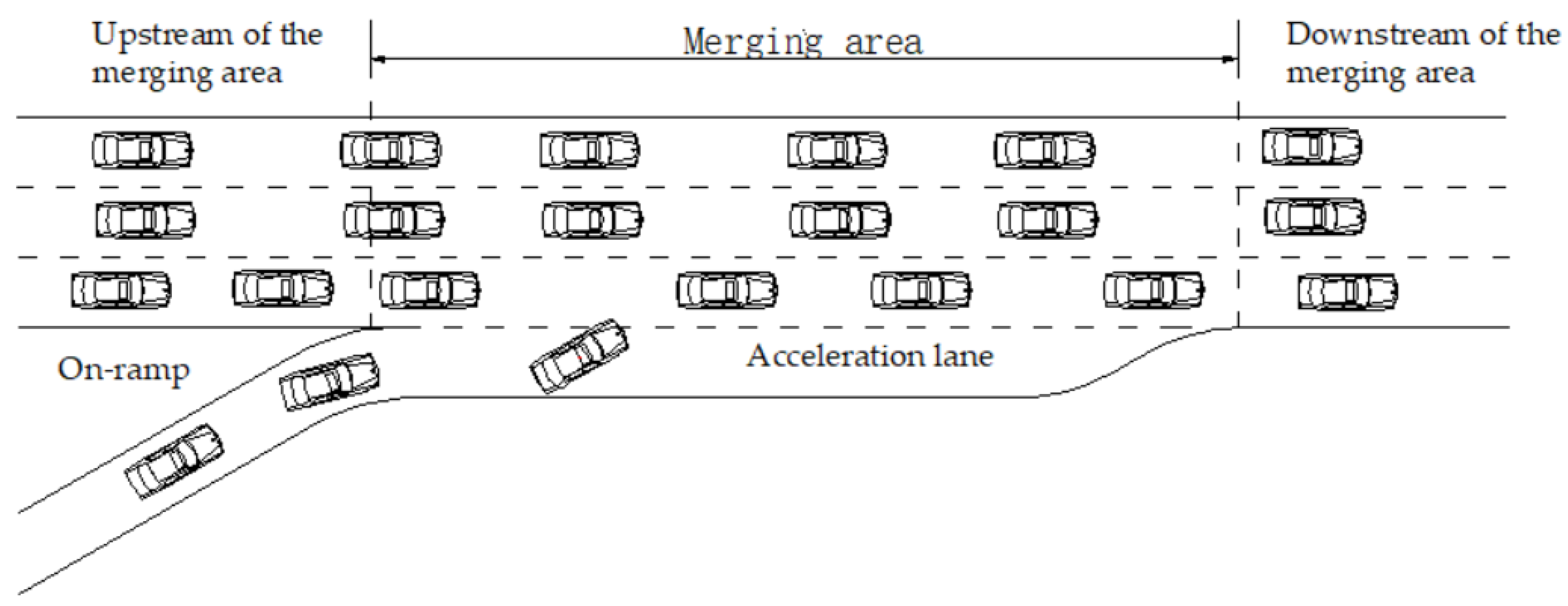
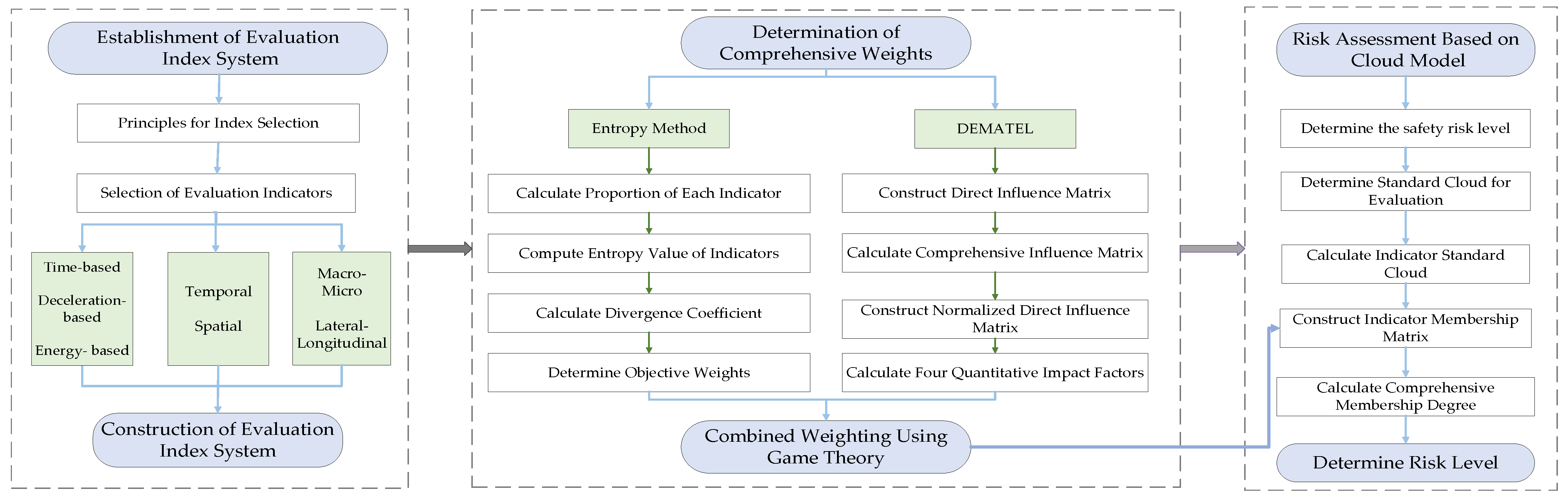
3.1. Framework of the Evaluation System

This study aims to evaluate the traffic safety of emerging mixed traffic flows in freeway merging areas under various scenarios. First, a comprehensive evaluation index system is established based on surrogate safety measures (SSMs), covering temporal, spatial, lateral-longitudinal, and micro-macro dimensions to fully capture the characteristics of traffic risk. Subsequently, objective weights are determined using the entropy method, while subjective weights are derived through the Decision-Making Trial and Evaluation Laboratory (DEMATEL) approach. These two sets of weights are then integrated using a game-theory combination strategy to ensure a balanced and scientifically grounded weighting scheme. Finally, a modified cloud model incorporating fuzzy clustering is constructed for risk assessment. Specifically, fuzzy c-means (FCM) clustering is employed to generate standard clouds for different risk levels, and reverse cloud generators are used to produce the evaluation clouds of indicators. The indicator weights are then integrated with the membership functions to compute the comprehensive membership degrees, which serve as the basis for determining the final risk level of each scenario. The overall evaluation framework is illustrated in Figure 2.

3.2. Establishment of Evaluation Index System

Considering the types of SSMs, this study selects six indicators to evaluate the traffic safety conditions in freeway merging areas from multiple dimensions, including time and space, lateral and longitudinal dynamics, as well as macro- and micro-level perspectives. These indicators include the following: Modified Time-to-Collision (MTTC), Lane Change Time-to-Collision (LCTTC), Deceleration Rate to Avoid a Crash (DRAC), Headway, Speed Standard Deviation (SD), and a newly proposed metric—Emergency Lane Change Risk Frequency (ELCRF), which represents the ratio of emergency lane changes to the total number of lane changes, considering the high frequency of lane changes and vehicle interactions in merging areas.

Detailed definitions and explanations of these six indicators are provided below.

• Modified Time to Collision (MTTC)

The Modified Time to Collision (MTTC) is an improved indicator used to assess longitudinal conflict risk in car-following scenarios. Unlike the traditional TTC, it incorporates the acceleration of both the leading and following vehicles, rather than assuming constant velocities [29]. This enhancement allows for a more realistic prediction of potential collision risks in dynamic traffic conditions. The MTTC is calculated using the following equation, and its conceptual illustration is provided in Figure 3.

$$\mathrm{MTTC}={\displaystyle \frac{-\Delta \mathrm{V}\pm \sqrt{{{\Delta \mathrm{V}}_{\mathrm{f}}}^2{+2\mathrm{a}}_{\mathrm{f}}\Delta \mathrm{D}}}{{\mathrm{a}}_{\mathrm{f}}}}$$

(1)

where $\Delta \mathrm{V}$ denotes the speed difference between the leading and following vehicles (m/s); ${\Delta \mathrm{V}}_{\mathrm{f}}$ represents the speed of the following vehicle (m/s); ${\mathrm{a}}_{\mathrm{f}}$ denotes the acceleration of the following vehicle (m/s²); and $\Delta \mathrm{D}$ is the distance between the leading vehicle and the following vehicle (m).

2.

Lane Change Time to Collision (LCTTC)

Lane Change Time to Collision (LCTTC) is an indicator used to assess lateral conflict risk during lane-changing maneuvers. It is defined as the time remaining until a potential lateral collision occurs between a lane-changing vehicle and a vehicle in the target lane, assuming both maintain their current speeds and trajectories [30]. This metric captures the dynamics of side-by-side interactions, which are critical in merging and overtaking scenarios. The calculation equations are as follows, and a schematic illustration of the lateral conflict scenario is provided in Figure 4.

$$\mathrm{LCTTC}=-{\displaystyle \frac{{\mathrm{d}}_{\mathrm{a},\mathrm{b}}}{{\mathrm{V}}_{\mathrm{a},\mathrm{b}}}}=-{\displaystyle \frac{{\left({\mathrm{P}}_{\mathrm{b}}-{\mathrm{P}}_{\mathrm{a}}\right)}^{\mathrm{T}}\times \left({\mathrm{P}}_{\mathrm{b}}-{\mathrm{P}}_{\mathrm{a}}\right)}{{\left({\mathrm{P}}_{\mathrm{b}}-{\mathrm{P}}_{\mathrm{a}}\right)}^{\mathrm{T}}\times \left({\mathrm{V}}_{\mathrm{b}}-{\mathrm{V}}_{\mathrm{a}}\right)}}$$

(2)

$${\mathrm{d}}_{\mathrm{a},\mathrm{b}}=\sqrt{{\left({\mathrm{P}}_{\mathrm{b}}-{\mathrm{P}}_{\mathrm{a}}\right)}^{\mathrm{T}}\times \left({\mathrm{P}}_{\mathrm{b}}-{\mathrm{P}}_{\mathrm{a}}\right)}$$

(3)

$${\mathrm{V}}_{\mathrm{a},\mathrm{b}}={\displaystyle \frac{1}{{\mathrm{d}}_{\mathrm{a},\mathrm{b}}}}{\left({\mathrm{P}}_{\mathrm{b}}-{\mathrm{P}}_{\mathrm{a}}\right)}^{\mathrm{T}}\times \left({\mathrm{P}}_{\mathrm{b}}-{\mathrm{P}}_{\mathrm{a}}\right)$$

(4)

where ${\mathrm{d}}_{\mathrm{a},\mathrm{b}}$ is distance between the lane-changing vehicle and vehicle in target lane (m); ${\mathrm{V}}_{\mathrm{a},\mathrm{b}}$ denotes the relative speed of the two vehicles (m/s); ${\mathrm{P}}_{\mathrm{b}}=\left({\mathrm{x}}_{\mathrm{b}}{,\mathrm{y}}_{\mathrm{b}}\right)$ is the position vector of the vehicle in the target lane; ${\mathrm{P}}_{\mathrm{a}}=\left({\mathrm{x}}_{\mathrm{a}}{,\mathrm{y}}_{\mathrm{a}}\right)$ indicates the position vector of the lane-changing vehicle; ${\mathrm{V}}_{\mathrm{b}}$ represents the velocity vector of the vehicle in the target lane; and ${\mathrm{V}}_{\mathrm{a}}$ represents the velocity vector of the lane-changing vehicle.

3.

Deceleration Rate to Avoid a Crash (DRAC)

DRAC is an indicator used to evaluate longitudinal conflict risk. It refers to the minimum required deceleration that a vehicle must apply to avoid a collision, assuming that the conflicting target vehicle maintains its current speed and trajectory [31]. This metric helps assess critical braking situations in car-following scenarios. It is expressed by the following equation, and a schematic diagram illustrating the longitudinal conflict scenario is provided in Figure 5:

$$\mathrm{DRAC}\left(\mathrm{t}\right)={\displaystyle \frac{{\left[\left({\mathrm{v}}_{\mathrm{i}}\left(\mathrm{t}\right)-{\mathrm{v}}_{\mathrm{i}-1}\left(\mathrm{t}\right)\right)\right]}^2}{2\left[{\mathrm{x}}_{\mathrm{i}-1}\left(\mathrm{t}\right)-{\mathrm{x}}_{\mathrm{i}}\left(\mathrm{t}\right)-{\mathrm{l}}_{\mathrm{i}-1}\right]}}$$

(5)

where ${\mathrm{v}}_{\mathrm{i}}\left(\mathrm{t}\right)$ is the speed of the following vehicle at time $\mathrm{t}$ (m/s); ${\mathrm{v}}_{\mathrm{i}-1}\left(\mathrm{t}\right)$ represents the speed of the leading vehicle at time $\mathrm{t}$ (m/s); ${\mathrm{x}}_{\mathrm{i}-1}\left(\mathrm{t}\right)$ denotes the position of the leading vehicle at time $\mathrm{t}$ (m); ${\mathrm{x}}_{\mathrm{i}}\left(\mathrm{t}\right)$ is the position of the following vehicle at time $\mathrm{t}$ (m); and ${\mathrm{l}}_{\mathrm{i}-1}$ is the length of the leading vehicle (m).

4.

Time Headway

Time Headway (TH) is defined as the time interval between two consecutive vehicles in the same lane as they pass a fixed point [32]. TH is calculated using Equation (6):

$${\mathrm{TH}=\mathrm{t}}_{\mathrm{i}}-{\mathrm{t}}_{\mathrm{i}-1}$$

(6)

where ${\mathrm{t}}_{\mathrm{i}}$ is the moment when the $\mathrm{ith}$ vehicle passes the fixed point; and ${\mathrm{t}}_{\mathrm{i}-1}$ is the moment when the $\left(\mathrm{i}-1\right)\mathrm{th}$ vehicle passes the fixed point.

5.

Speed Standard Deviation (SD)

Speed standard deviation (SD) is a statistic used to describe the degree of dispersion of vehicle speed distribution. The greater the standard deviation of vehicle speeds, the more pronounced the asymmetry in traffic flow, reflecting a higher variability in vehicle behavior, which is more likely to increase safety risks. The SD of the traffic flow is calculated by the following equation [33]:

$$\mathsf{\sigma }=\sqrt{{\displaystyle \frac{{{\displaystyle {\sum }_{\mathrm{i}=1}^{\mathrm{N}}\left({\mathrm{v}}_{\mathrm{i}}-\overline{\mathrm{v}}\right)}}^2}{\mathrm{N}-1}}}$$

(7)

where $\mathrm{N}$ denotes the total number of vehicles (veh); ${\mathrm{v}}_{\mathrm{i}}$ represents the speed of vehicle $\mathrm{i}$ (m/s); and $\overline{\mathrm{v}}$ is the average speed of all vehicles (m/s).

6.

Emergency-Lane-change Risk Frequency (ELCRF)

Emergency Lane-Change Risk Frequency (ELCRF) is a behavioral indicator that indirectly reflects lateral conflict risk through urgent lane-change behavior. It is defined as the ratio of the number of emergency lane changes to the total number of lane changes occurring in the merging area at time step t. Emergency lane changes refer to maneuvers that must be executed urgently, typically due to imminent conflict, congestion avoidance, or safety enhancement needs. These lane-change requests are characterized by a higher priority and greater immediacy compared to regular lane changes. A lower ELCRF value indicates a more stable and orderly traffic flow in the merging area, and thus a higher level of safety. The ELCRF is calculated using the following equation, and a schematic diagram of the associated longitudinal risk behavior is provided in Figure 6:

$$\mathrm{ELCRF}\left(\mathrm{t}\right)={\displaystyle \frac{{\mathrm{n}}_{\mathrm{e}}\left(\mathrm{t}\right)}{{\mathrm{n}}_{\mathrm{t}}\left(\mathrm{t}\right)}}$$

(8)

where ${\mathrm{n}}_{\mathrm{e}}\left(\mathrm{t}\right)$ denotes the number of emergency lane changes; and ${\mathrm{n}}_{\mathrm{t}}\left(\mathrm{t}\right)$ is the total number of lane changes.

From a longitudinal and lateral perspective—and based on traditional Surrogate Safety Measures (SSM)—time-related indicators such as MTTC (collision time), headway (time gap), and LCTTC (lateral collision time) are selected. DRAC (deceleration rate) is used to measure the deceleration required to avoid a collision, evaluating a driver’s ability to react to potential collision risks and reflecting overall driving safety. ELCRF effectively captures the intensity of vehicle interactions, which is closely related to the energy aspect of Surrogate Safety Measures (SSM), as it reflects the potential collision energy involved when vehicles perform emergency lane changes. Additionally, considering the micro-level focus on individual vehicle behavior in the traffic flow, Speed Standard Deviation (SD) was chosen as a macro-level indicator to assess the overall traffic conditions and stability of the traffic flow.

By considering time-domain aspects, deceleration, and interaction severity (ELCRF), along with longitudinal and lateral dynamics, as well as macro- and micro-level perspectives, this study establishes a comprehensive and integrated system of indicators for evaluating traffic safety in freeway merging areas, as listed in

Table 1. Indicator characteristics for traffic safety evaluations.

Indicator	Types of SSMs			Dimension		Scale		Time-Space
	Time-Based	Deceleration-Based	Energy Based	Longitudinal Dynamics	Lateral Dynamics	Macro-Level	Micro-Level	Temporal	Spatial
MTTC	✓			✓			✓	✓
LCTTC	✓				✓		✓	✓
DRAC		✓		✓			✓		✓
SD						✓			✓
Headway	✓			✓			✓	✓
ELCRF			✓		✓		✓		✓

.

3.3. Determination of Weight of Index

As the importance of each evaluation indicator varies, appropriate weighting is essential for accurate and balanced assessments. This study combines both subjective and objective weighting methods to ensure reliability. Specifically, the entropy method is used to compute objective weights based on data variability, while the Decision-Making Trial and Evaluation Laboratory (DEMATEL) method derives subjective weights from expert judgment. To unify these differing perspectives, an improved game theory-based combination method is applied to obtain comprehensive weights for the final evaluation. This integration aims to ensure a balanced and symmetrical evaluation outcome.

3.3.1. Calculating Objective Weights by Entropy Method

The entropy method [34] is a widely used multi-criteria decision-making technique derived from information theory. It is particularly suitable for complex, multi-dimensional datasets where prior knowledge of index importance is lacking. This method calculates the entropy value of each evaluation indicator to quantify its degree of variation, thereby determining its weight in the comprehensive evaluation. A lower entropy value indicates greater variability, and thus a higher weight; conversely, a higher entropy value suggests lower variability and contributes less to the overall assessment. The calculation process involves the following steps:

Step 1: Establish the original data matrix.

The number of existing projects to be evaluated is assumed to be n, and the number of evaluation indexes is m. The original data matrix of the evaluation index corresponding to the project to be evaluated is as follows:

$${\mathrm{X}}_{\mathrm{ij}}={\left({\mathrm{x}}_{\mathrm{ij}}\right)}_{\mathrm{n}\times \mathrm{m}}=\left[\begin{array}{ccc}{\mathrm{x}}_{11}& \dots & {\mathrm{x}}_{1\mathrm{j}}\\ \dots & \dots & \dots \\ {\mathrm{x}}_{\mathrm{n}1}& \dots & {\mathrm{x}}_{\mathrm{nm}}\end{array}\right]$$

(9)

where ${\mathrm{x}}_{\mathrm{ij}}$ represents raw data of the $\mathrm{ith}$ evaluation object on the $\mathrm{jth}$ indicator.

Step 2: Normalize the raw data for each evaluation indicator

To eliminate the influence of different units and scales, the raw data for each evaluation indicator is normalized using the following formula:

$${\mathrm{x}}_{\mathrm{ij}}^{\prime }={\displaystyle \left\{\begin{array}{l}\frac{{\mathrm{x}}_{\mathrm{ij}}-\min \left({\mathrm{x}}_{\mathrm{j}}\right)}{\max \left({\mathrm{x}}_{\mathrm{j}}\right)-\min \left({\mathrm{x}}_{\mathrm{j}}\right)},\mathrm{if}\mathrm{the}\mathrm{indicator}\mathrm{is}\mathrm{positively}\mathrm{oriented}\\ \frac{\max \left({\mathrm{x}}_{\mathrm{j}}\right)-{\mathrm{x}}_{\mathrm{ij}}}{\max \left({\mathrm{x}}_{\mathrm{j}}\right)-\min \left({\mathrm{x}}_{\mathrm{j}}\right)},\mathrm{if}\mathrm{the}\mathrm{indicator}\mathrm{is}\mathrm{negatively}\mathrm{oriented}\end{array}\right.}$$

(10)

where ${\mathrm{x}}_{\mathrm{ij}}$ represents raw data; ${\mathrm{x}}_{\mathrm{ij}}^{\prime }$ denotes the standardized value of the $\mathrm{ith}$ evaluation object on the $\mathrm{jth}$ index, and the resulting normalized values ${\mathrm{x}}_{\mathrm{ij}}^{\prime }$ fall within the range [0, 1]; $\max \left({\mathrm{x}}_{\mathrm{j}}\right)$ means the maximum value of the $\mathrm{jth}$ index; and $\min \left({\mathrm{x}}_{\mathrm{j}}\right)$ means the minimum value of the $\mathrm{jth}$ index.

Then, the matrix after standardization can be expressed as follows:

$${\mathrm{X}}_{\mathrm{ij}}^{\prime }={\left({\mathrm{x}}_{\mathrm{ij}}^{\prime }\right)}_{\mathrm{n}\times \mathrm{m}}=\left[\begin{array}{ccc}{\mathrm{x}}_{11}^{\prime }& \dots & {\mathrm{x}}_{1\mathrm{j}}^{\prime }\\ \dots & \dots & \dots \\ {\mathrm{x}}_{\mathrm{n}1}^{\prime }& \dots & {\mathrm{x}}_{\mathrm{nm}}^{\prime }\end{array}\right]$$

(11)

Step 3: Calculate the proportion of each indicator

The proportion ${\mathrm{y}}_{\mathrm{ij}}$ of the $\mathrm{jth}$ indicator under the $\mathrm{ith}$ evaluation object is calculated as:

$${\mathrm{y}}_{\mathrm{ij}}={\displaystyle \frac{{\mathrm{x}}_{\mathrm{ij}}^{\prime }}{{\displaystyle \sum _{\mathrm{i}=1}^{\mathrm{m}}{\mathrm{x}}_{\mathrm{ij}}^{\prime }}}}$$

(12)

Step 4: Compute the entropy value of each indicator

The entropy value ${\mathrm{e}}_{\mathrm{j}}$ for each indicator is given by the following:

$${\mathrm{e}}_{\mathrm{j}}=-\mathrm{k}{\displaystyle \sum _{\mathrm{i}=1}^{\mathrm{m}}\left({\mathrm{y}}_{\mathrm{ij}}\times {\ln \mathrm{y}}_{\mathrm{ij}}\right)}{,\mathrm{y}}_{\mathrm{ij}}>0$$

(13)

where $\mathrm{k}$ is a normalization constant, generally taken as $\mathrm{k}={\displaystyle \frac{1}{\ln \mathrm{m}}}$.

Step 5: Calculate the redundancy (degree of divergence)

The redundancy ${\mathrm{d}}_{\mathrm{j}}$ of entropy is calculated as:

$${\mathrm{d}}_{\mathrm{j}}=1-{\mathrm{e}}_{\mathrm{j}}$$

(14)

Step 6: Determine the objective weight of each indicator

Finally, the objective weight ${\mathrm{w}}_{\mathrm{j}}$ of the $\mathrm{jth}$ indicator is calculated as:

$${\mathrm{w}}_{\mathrm{j}}={\displaystyle \frac{{\mathrm{d}}_{\mathrm{j}}}{{\displaystyle \sum _{\mathrm{j}=1}^{\mathrm{n}}{\mathrm{d}}_{\mathrm{j}}}}}$$

(15)

3.3.2. Calculating Subjective Weights by the DEMATEL Method

The Decision-Making Trial and Evaluation Laboratory (DEMATEL) method is a system analysis technique based on graph theory and matrix operations, originally proposed by A. Gabus and E. Fontela at the Battelle Memorial Institute, Ohio, USA in 1971 [35]. It is widely used to explore and quantify causal relationships among factors in complex systems. By constructing a direct influence matrix, the DEMATEL method reveals both direct and indirect interactions between elements through matrix computations. In addition to identifying the strength of relationships, it can also determine key influencing factors by calculating indicators such as influence degree, influenced degree, centrality, and cause degree.

The detailed steps for calculating subjective weights using DEMATEL are as follows:

Step 1: collect expert opinions and calculate the average direct influence of matrix E.

In this step, the expert’s judgments on the degree of influence between pairs of factors are collected. The degree of influence of factor $\mathrm{i}$ on factor $\mathrm{j}$ is expressed as ${\mathrm{x}}_{\mathrm{ij}}$, which is assessed using a scale ranging from 0 to 4 (i.e., 0 = no impact; 1 = slight impact; 2 = moderate impact; 3 = noticeable impact; 4 = obvious impact). For expert k, there is a judgment matrix ${\mathrm{X}}^{\mathrm{k}}=\left[{\mathrm{x}}_{\mathrm{ij}}^{\mathrm{k}}\right]$, k = (1, 2, …, m), then the average judgment matrix E of all experts is integrated as follows:

$${\mathrm{E}}_{\mathrm{ij}}={\displaystyle \frac{1}{\mathrm{m}}}{\displaystyle \sum _{\mathrm{i}=1}^{\mathrm{m}}{\mathrm{x}}_{\mathrm{ij}}^{\mathrm{k}}}$$

(16)

Step 2: Normalize the direct influence matrix E.

To ensure comparability, the direct influence matrix is normalized using the maximum row sum method. The normalized matrix F is calculated as:

$$\mathrm{F}=\left[{\displaystyle \frac{{\mathrm{x}}_{\mathrm{ij}}}{\max {\displaystyle \sum _{\mathrm{j}=1}^{\mathrm{m}}{\mathrm{x}}_{\mathrm{ij}}}}}\right]$$

(17)

Step 3: Construct the total influence matrix T

The total (comprehensive) influence matrix T includes both direct and indirect influences, and is calculated as:

$$\mathrm{T}=\mathrm{F}\times {(\mathrm{I}-\mathrm{F})}^{-1}$$

(18)

where $\mathrm{I}$ denotes unit matrix.

Step 4: calculate influence degree ${\mathrm{D}}_{\mathrm{i}}$, influenced degree ${\mathrm{C}}_{\mathrm{i}}$, centrality ${\mathrm{M}}_{\mathrm{i}}$, and cause degree ${\mathrm{R}}_{\mathrm{i}}$.

The influence degree ${\mathrm{D}}_{\mathrm{i}}$ represents the total effect that element $\mathrm{i}$ has on all other elements:

$${\mathrm{D}}_{\mathrm{i}}={\displaystyle {\sum }_{\mathrm{j}=1}^{\mathrm{n}}{\mathrm{T}}_{\mathrm{ij}}}$$

(19)

The influenced degree ${\mathrm{C}}_{\mathrm{i}}$ is the total effect that element i receives from others:

$${\mathrm{C}}_{\mathrm{i}}={\displaystyle {\sum }_{\mathrm{j}=1}^{\mathrm{n}}{\mathrm{T}}_{\mathrm{ji}}}$$

(20)

Centrality ${\mathrm{M}}_{\mathrm{i}}$ is the sum of influence and influenced degrees, reflecting the overall importance of an element:

$${\mathrm{M}}_{\mathrm{i}}{=\mathrm{D}}_{\mathrm{i}}{+\mathrm{C}}_{\mathrm{i}}$$

(21)

Cause degree ${\mathrm{R}}_{\mathrm{i}}$ is the difference between the influence and influenced degrees, used to classify the role of the element:

$${\mathrm{R}}_{\mathrm{i}}{=\mathrm{D}}_{\mathrm{i}}-{\mathrm{C}}_{\mathrm{i}}$$

(22)

If ${\mathrm{R}}_{\mathrm{i}}>0$, the indicator is a cause element; otherwise, it is a result element.

Step 5: Calculate the subjective weight of each indicator

The subjective weight ${\mathrm{w}}_{\mathrm{i}}$ of indicator $\mathrm{i}$ is derived from its centrality using the following normalization:

$${\mathrm{w}}_{\mathrm{i}}={\displaystyle \frac{\sqrt{{\mathrm{M}}_{\mathrm{i}}^2{+\mathrm{R}}_{\mathrm{i}}^2}}{{\displaystyle {\sum }_{\mathrm{j}=1}^{\mathrm{n}}\sqrt{{\mathrm{M}}_{\mathrm{i}}^2{+\mathrm{R}}_{\mathrm{i}}^2}}}}$$

(23)

3.3.3. Calculating Final Weights Using Game Theory

The entropy method relies solely on objective data, neglecting the insights and experience of experts and decision-makers, which may result in evaluations that fail to fully reflect real-world conditions. In contrast, the DEMATEL method incorporates subjective knowledge and practical application scenarios, but may suffer from a high degree of subjectivity and randomness. To address these limitations, it is necessary to integrate both subjective and objective weighting approaches. Game theory provides a framework to dynamically balance these two types of weights by simulating the cooperation and competition between indicators, thereby achieving optimal weighting effects. However, conventional game theory methods may generate negative combination coefficients, which can hinder the interpretability and validity of the final weights. To overcome this issue, this study introduces non-negativity constraints to improve the game-theory-based weight combination process. The detailed calculation steps are outlined as follows:

Step 1: Establish a linear combination model for integrated weights

The final comprehensive weight vector ${\mathrm{w}}_{\mathrm{c}}$ is obtained through a linear combination of weights derived from multiple methods:

$${\mathrm{w}}_{\mathrm{c}}={\displaystyle \sum _{\mathrm{k}=1}^{\mathrm{K}}{\mathsf{\beta }}_{\mathrm{k}}{\mathrm{w}}_{\mathrm{k}}^{\mathrm{T}}}$$

(24)

where $\mathrm{K}$ denotes the total number of methods; ${\mathrm{w}}_{\mathrm{k}}$ denotes weight obtained by method k; ${\mathsf{\beta }}_{\mathrm{k}}$ means the coefficient of weight and ${\mathsf{\beta }}_{\mathrm{k}}\ge 0$; and ${\mathrm{w}}_{\mathrm{k}}^{\mathrm{T}}$ represents the transpose of the weighted row vector.

Step 2: Formulate the optimization model

An optimization model is established with the objective of minimizing the deviation between the comprehensive weight ${\mathrm{w}}_{\mathrm{c}}$ and the weight ${\mathrm{w}}_{\mathrm{k}}$ of each method. The optimization model is defined as follows:

$$\min {‖{\displaystyle \sum _{\mathrm{k}=1}^{\mathrm{K}}{\mathsf{\beta }}_{\mathrm{k}}{\mathrm{w}}_{\mathrm{k}}^{\mathrm{T}}-{\mathrm{w}}_{\mathrm{i}}^{\mathrm{T}}}‖}_2,\mathrm{i}=1,2,\dots ,\mathrm{k}$$

(25)

Step 3: Introduce non-negativity and normalization constraints

To ensure interpretability and validity of the solution, the following constraints are added:

$${\displaystyle \sum _{\mathrm{k}=1}^{\mathrm{K}}{\mathsf{\beta }}_{\mathrm{k}}^2=1,}{\mathsf{\beta }}_{\mathrm{k}}>0$$

(26)

Step 4: Construct and solve the Lagrange function

To solve the constrained optimization problem, the Lagrange function is constructed as follows:

$$\mathsf{\Gamma }\left({\mathsf{\beta }}_1{,\mathsf{\beta }}_2,\dots {,\mathsf{\beta }}_{\mathrm{K}},\mathsf{\lambda }\right)={\displaystyle \sum _{\mathrm{i}=1}^{\mathrm{K}}‖{\displaystyle \sum _{\mathrm{k}=1}^{\mathrm{K}}{\mathsf{\beta }}_{\mathrm{k}}{\mathrm{w}}_{\mathrm{i}}{\mathrm{w}}_{\mathrm{k}}^{\mathrm{T}}-}{\mathrm{w}}_{\mathrm{i}}{\mathrm{w}}_{\mathrm{i}}^{\mathrm{T}}‖}+{\displaystyle \frac{\mathsf{\lambda }}{2}}\left({\displaystyle \sum _{\mathrm{k}=1}^{\mathrm{K}}{\mathsf{\beta }}_{\mathrm{k}}^2-1}\right)$$

(27)

where $\lambda$ denotes Lagrange multiplier, reflecting the influence of constraints on the objective function.

The partial derivatives of the Lagrange function with respect to the combination coefficients ${\mathsf{\beta }}_{\mathrm{k}}$ and the constraint variables $\mathsf{\lambda }$ are set to be zero, and the conditions for the existence of extreme values are obtained, as shown in Equations (28) and (29):

$${\displaystyle \frac{\mathsf{\partial }\mathsf{\Gamma }}{\mathsf{\partial }{\mathsf{\beta }}_{\mathrm{k}}}}={\displaystyle {\sum }_{\mathrm{i}=1}^{\mathrm{K}}\left|{\mathrm{w}}_{\mathrm{i}}{\mathrm{w}}_{\mathrm{k}}^{\mathrm{T}}\right|}{+\mathsf{\lambda }\mathsf{\beta }}_{\mathrm{k}}=0$$

(28)

$${\displaystyle \frac{\mathsf{\partial }\mathsf{\Gamma }}{\mathsf{\partial }\mathsf{\lambda }}}={\displaystyle {\sum }_{\mathrm{k}=1}^{\mathrm{K}}{\mathsf{\beta }}_{\mathrm{k}}^2-1}=0$$

(29)

The optimal solution of the combined coefficients is obtained by solving the above equations, as shown in Equation (30).

$${\mathsf{\beta }}_{\mathrm{k}}={\displaystyle \frac{{\displaystyle {\sum }_{\mathrm{i}=1}^{\mathrm{K}}{\mathrm{w}}_{\mathrm{i}}{\mathrm{w}}_{\mathrm{k}}^{\mathrm{T}}}}{\sqrt{{\displaystyle {\sum }_{\mathrm{k}=1}^{\mathrm{K}}{\left({\displaystyle {\sum }_{\mathrm{i}=1}^{\mathrm{K}}{\mathrm{w}}_{\mathrm{i}}{\mathrm{w}}_{\mathrm{k}}^{\mathrm{T}}}\right)}^2}}}}$$

(30)

Step 5: Calculate and normalize the final comprehensive weights

The obtained solution ${\mathsf{\beta }}_{\mathrm{k}}$ is substituted into the formula (24) to obtain the comprehensive weight ${\mathrm{w}}_{\mathrm{c}}=\left({\mathrm{w}}_{\mathrm{c}1}{,\mathrm{w}}_{\mathrm{c}2},\dots {,\mathrm{w}}_{\mathrm{cn}}\right)$. To ensure that the sum of the weights is 1, the comprehensive weight is normalized by the following formula:

$${\mathrm{w}}_{\mathrm{dj}}={\displaystyle \frac{{\mathrm{w}}_{\mathrm{cj}}}{{\displaystyle {\sum }_{\mathrm{j}=1}^{\mathrm{n}}{\mathrm{w}}_{\mathrm{cj}}}}}$$

(31)

where ${\mathrm{w}}_{\mathrm{cj}}$ denoted the comprehensive weight of index $\mathrm{j}$.

This combined weighting method effectively bridges expert judgment and data-driven analysis. The entropy method captures the objective variation in the data, while DEMATEL reflects the expert understanding of inter-indicator influences. Game theory harmonizes these two sources, optimizing their contributions while preventing bias or dominance. By integrating both perspectives under a unified, constraint-based optimization framework, this method enhances the robustness, realism, and interpretability of the final weights.

3.4. Comprehensive Evaluation of Cloud Model Based on Fuzzy Clustering

3.4.1. Cloud Model Theory

The cloud model is a mathematical model proposed by Academician Li Deyi in 1995 [36] based on fuzzy set theory and probability theory, which effectively addresses uncertainty issues in the evaluation process. It facilitates the transformation between qualitative concepts and quantitative characteristics through the use of a cloud generator. The cloud model consists of numerous cloud droplets, each representing a specific point within the distribution of a quantitative domain. The model is characterized by three key digital features: expected value (Ex), entropy (En), and hyper-entropy (He). Ex represents the central value of the cloud droplets within the quantitative domain, while En measures the randomness of the qualitative concepts, reflecting the degree of dispersion of the cloud droplets. He indicates the dispersion of the entropy (En), representing the “thickness” of the cloud.

The membership function of a cloud model measures the membership of a value to a specific cloud model, as shown in Equation (32).

$$\mathrm{u}\left(\mathrm{x}\right){=\mathrm{e}}^{-{\displaystyle \frac{{\left(\mathrm{x}-\mathrm{Ex}\right)}^2}{{2\mathrm{En}}^2}}}$$

(32)

where $\mathrm{x}$ denotes a value in the quantitative domain; and $\mathrm{u}\left(\mathrm{x}\right)$ is the degree of membership that the value belongs to the corresponding qualitative concept.

3.4.2. Modified Cloud Model

Fuzzy C-means (FCM) clustering analysis can effectively deal with the uncertainty and fuzziness of the data by optimizing the objective function and identifying the fuzzy patterns in the data [37], while the cloud model can better describe the central trend, dispersion and fuzziness of the data through the three parameters of expected value, entropy, and hyper entropy. Hence, this study combines fuzzy clustering with the cloud model to estimate the traffic safety of mixed traffic flow. The specified processes are as follows.

Step 1: Define safety levels and normalize index data

According to the Technical Specification for Risk Assessment of Highway Traffic Safety, the safety risk is divided into five levels: high risk (level 1), moderate risk (level 2), average risk (level 3), low risk (level 4), and very low risk (level 5). This classification is widely adopted in national traffic safety assessments and serves as a standard framework for evaluating road safety performance in China. To ensure that all indicators are compared on the same scale, the indicators are homogenized and normalized. The calculation equations are expressed by Equation (10).

Step 2: Determine the criteria cloud of indicators

FCM clustering is a soft clustering algorithm based on objective function optimization, and its core idea is to describe the relationship between sample points and cluster centers through membership function [37]. Compared to traditional hard clustering, FCM allows data points to belong to multiple clusters with varying degrees of membership, making it more suitable for handling the fuzzy characteristics of risk levels in traffic safety evaluations. In this study, FCM is employed to obtain the cluster centers, which serve as the expected values for each risk level.

To assign the risk levels (high, moderate, average, low, and very low), the cluster centers derived from FCM are utilized to determine the thresholds for each level. Once the cluster centers are determined, they are further used to calculate the entropy and hyper-entropy, which are key parameters of the cloud model. These parameters help quantify the risk characteristics of each level and define the risk thresholds. The thresholds for each of the five levels are derived based on the cloud model parameters, ensuring a data-driven and contextually justified classification. This approach accounts for the inherent uncertainties in the evaluation process, offering a comprehensive and accurate risk level assignment.

The objective function of FCM is defined as follows:

$$\mathrm{J}={{\displaystyle \sum _{\mathrm{i}=1}^{\mathrm{n}}{\displaystyle \sum _{\mathrm{j}=1}^{\mathrm{c}}{\mathrm{u}}_{\mathrm{ij}}^{\mathrm{m}}‖{\mathrm{x}}_{\mathrm{i}}-{\mathrm{v}}_{\mathrm{j}}‖}}}^2$$

(33)

where ${\mathrm{u}}_{\mathrm{ij}}$ denotes the membership matrix element; $\mathrm{n}$ is the total number of data points; $\mathrm{c}$ indicates the number of clusters; ${\mathrm{x}}_{\mathrm{i}}$ is the feature vector of data point $\mathrm{i}$; ${\mathrm{v}}_{\mathrm{j}}$ is the center of cluster $\mathrm{j}$; $\mathrm{m}$ represents the fuzz factor; and $‖{\mathrm{x}}_{\mathrm{i}}-{\mathrm{v}}_{\mathrm{j}}‖$ denotes the Euclidean distance between data point $\mathrm{i}$ and cluster center $\mathrm{j}$.

The center of the cluster is obtained by the following steps:

• Initialization: Construct the initial membership matrix ${\mathrm{U}}^{\left(0\right)}$ ensuring ${\displaystyle {\sum }_{\mathrm{j}=1}^{\mathrm{c}}{\mathrm{u}}_{\mathrm{ij}}=1}$
• Calculate the cluster center

According to the membership matrix ${\mathrm{U}}^{\left(0\right)}$ and the data points, the center position of each cluster is calculated by the following formula.

$${\mathrm{v}}_{\mathrm{j}}={\displaystyle \frac{{\displaystyle {\sum }_{\mathrm{i}=1}^{\mathrm{n}}{\mathrm{u}}_{\mathrm{ij}}^{\mathrm{m}}{\mathrm{x}}_{\mathrm{i}}}}{{\displaystyle {\sum }_{\mathrm{i}=1}^{\mathrm{n}}{\mathrm{u}}_{\mathrm{ij}}^{\mathrm{m}}}}}$$

(34)

3.

Update membership matrix

According to the current cluster center, the membership degree of each data point to each cluster is recalculated by Equation (35).

$${\mathrm{u}}_{\mathrm{ij}}={\left[{\displaystyle \sum _{\mathrm{k}=1}^{\mathrm{c}}{\left(\frac{‖{\mathrm{x}}_{\mathrm{i}}-{\mathrm{v}}_{\mathrm{j}}‖}{‖{\mathrm{x}}_{\mathrm{i}}-{\mathrm{v}}_{\mathrm{k}}‖}\right)}^{\frac{2}{\mathrm{m}-1}}}\right]}^{-1}$$

(35)

4.

Iteration: Repeat Steps 2–3 until convergence; i.e., when the change in objective function satisfies $\left|{\mathrm{J}}^{\left(\mathrm{t}\right)}-{\mathrm{J}}^{\left(\mathrm{t}-1\right)}\right|<\mathsf{\epsilon }$, where ${\mathsf{\epsilon }=10}^{-5}$.

5.

Output result: The final cluster centers ${\mathrm{v}}_{\mathrm{j}}$ are taken as the expected values ${\mathrm{Ex}}_{\mathrm{standard}}$ of the cloud model. Then, the entropy ${\mathrm{En}}_{\mathrm{standard}}$ and hyper-entropy ${\mathrm{He}}_{\mathrm{standard}}$ are calculated as:

$${\mathrm{En}}_{\mathrm{standard}}=\sqrt{{\displaystyle \frac{{\displaystyle {\sum }_{\mathrm{i}=1}^{\mathrm{n}}{\mathrm{u}}_{\mathrm{ij}}^2{\left({\mathrm{x}}_{\mathrm{i}}-{\mathrm{Ex}}_{\mathrm{j}}\right)}^2}}{{\displaystyle {\sum }_{\mathrm{i}=1}^{\mathrm{n}}{\mathrm{u}}_{\mathrm{ij}}^2}}}}$$

(36)

$${\mathrm{He}}_{\mathrm{standard}}=\mathrm{k}\times {\mathrm{En}}_{\mathrm{standard}}$$

(37)

where ${\mathrm{Ex}}_{\mathrm{j}}$ denotes the expected value of cluster $\mathrm{j}$; $\mathrm{k}$ is constant and taken as 0.1.

Step 3: Calculate the cloud parameters for each alternative scheme

For each evaluation scheme, the expected value, entropy, and hyper-entropy of each indicator are calculated using a backward cloud generator:

$${\mathrm{Ex}}_{\mathrm{i}}={\displaystyle \frac{1}{\mathrm{n}}}{\displaystyle \sum _{\mathrm{i}=1}^{\mathrm{n}}{\mathrm{x}}_{\mathrm{s},\mathrm{i}}}$$

(38)

$${\mathrm{En}}_{\mathrm{i}}=\sqrt{{\displaystyle \frac{\mathsf{\pi }}{2}}}\times {\displaystyle \frac{1}{\mathrm{n}}}{\displaystyle \sum _{\mathrm{i}=1}^{\mathrm{n}}\left|{\mathrm{x}}_{\mathrm{s},\mathrm{i}}-{\mathrm{Ex}}_{\mathrm{i}}\right|}$$

(39)

where ${\mathrm{x}}_{\mathrm{s},\mathrm{i}}$ is the feature vector of data point $\mathrm{i}$ of scheme $\mathrm{s}$.

Step 4: Calculate the membership matrix and comprehensive membership degree

In order to quantify the proximity between the evaluation index of different schemes and each risk level, the fuzzy membership calculation method based on the cloud model is adopted [38]. Specifically, the expected value of the indicators of each scheme is mapped to the membership interval of [0, 1] through the exponential function, to measure the possibility of belonging to different risk levels. For the indicator i of each scheme s, its membership to the risk level j is calculated by the following formula:

$${\mathrm{u}}_{\mathrm{s},\mathrm{i},\mathrm{k}}=\exp \left(-{\displaystyle \frac{{\left({\mathrm{Ex}}_{\mathrm{s},\mathrm{i}}-{\mathrm{Ex}}_{\mathrm{standard},\mathrm{i},\mathrm{k}}\right)}^2}{2{\left({\mathrm{En}}_{\mathrm{standard},\mathrm{i},\mathrm{k}}\right)}^2}}\right)$$

(40)

where ${\mathrm{Ex}}_{\mathrm{s},\mathrm{i}}$ denoted the expected value of index $\mathrm{i}$ of scheme s; ${\mathrm{Ex}}_{\mathrm{standard},\mathrm{i},\mathrm{k}}$ implies the standard expected value of index $\mathrm{i}$ in safety level k; and ${\mathrm{En}}_{\mathrm{standard},\mathrm{i},\mathrm{k}}$ is the standard entropy of index $\mathrm{i}$ in safety level k.

The comprehensive membership degree can be calculated by combining the membership matrix of each indicator and indicator weight as follows:

$${\mathrm{u}}_{\mathrm{s},\mathrm{k}}={\displaystyle {\sum }_{\mathrm{i}=1}^{\mathrm{m}}{\mathrm{u}}_{\mathrm{s},\mathrm{i},\mathrm{k}}}\times {\mathrm{w}}_{\mathrm{d},\mathrm{j}}$$

(41)

$${\mathrm{u}}_{\mathrm{s},\mathrm{k}}^{\prime }={\displaystyle \frac{{\mathrm{u}}_{\mathrm{s},\mathrm{k}}}{{\displaystyle {\sum }_{\mathrm{i}=1}^{\mathrm{n}}{\mathrm{u}}_{\mathrm{s},\mathrm{k}}}}}$$

(42)

where $\mathrm{m}$ denotes the total number of indicators; $\mathrm{n}$ is the safety level; ${\mathrm{w}}_{\mathrm{d},\mathrm{j}}$ represents the weight of indicator j; and ${\mathrm{u}}_{\mathrm{s},\mathrm{k}}^{\prime }$ is the comprehensive membership degree after normalization.

Step 5: Determine the safety level

According to the maximum membership principle, the safety level of the merging area is determined as the level corresponding to the highest normalized membership value.

4. Case Study

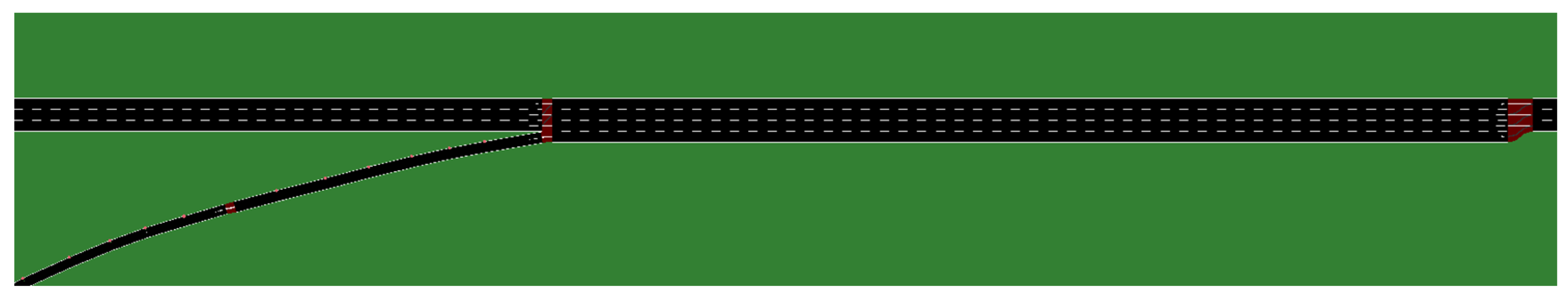
4.1. Simulation Design

Due to the lack of real-world autonomous vehicle (AV) data, this study aims to investigate the safety of mixed traffic flow at freeway merging areas using the SUMO simulation platform. A merging area with a single-lane parallel acceleration lane is selected as the simulation scenario. The main line consists of three lanes, while the ramp has a single lane with a width of 3.75 m, as shown in Figure 7. In this study, the traffic flow rates, ramp-to-mainline flow ratio, and AV penetration rates are selected as the influencing factors for simulating mixed traffic, using a full factorial experimental design. Traffic flow plays a crucial role in determining safety, as higher flow rates can exacerbate congestion and increase the likelihood of conflicts. Referring to the “Design Code for Urban Expressways” (CJJ37-2012 [39], 2016 edition) in China, three traffic flow rates (3000 pcu/h, 4500 pcu/h, 6000 pcu/h) are used to simulate low, medium, and high-flow traffic conditions. Disproportionate ramp-to-mainline ratios create merging asymmetry, leading to congestion and conflict, particularly in mixed traffic. Therefore, the ramp-to-mainline ratio is considered as one of the influencing factors. Typically, ramp flow does not exceed half of the mainline flow. Since the simulated ramp is a single-lane ramp, the ramp-to-mainline ratio is selected to range from 0.15 to 0.35, with a step size of 0.1. At 0% and 100% AV penetration, the traffic flow is symmetric, with either all HDVs or all AVs, leading to uniform behavior. As AV penetration increases, the flow becomes increasingly asymmetric, with HDVs initially dominating and interacting unpredictably with AVs. As AV penetration continues to rise, more AVs enter the flow, and HDVs start to mimic their behavior, shifting the flow towards an AV-dominated asymmetric system. Based on previous studies [17,40] on the impact of AV penetration rate on mixed traffic, this study chooses to change the AV penetration rate from 0 to 1 with a step of 0.2. Thus, a total of 54 simulation scenarios are designed. The intelligent driver model (IDM) and Adaptive Cruise Control (ACC) models have been proven to be effective in modelling HDVs and AVs in existing studies [19,41]. In addition, the default lane-changing model LC2013 in SUMO has also been utilized in past studies to simulate the lane-changing behavior of both HDVs and AVs [42,43]. Therefore, in this study, the IDM and ACC models as well as the LC2013 lane-changing model are adopted to simulate the driving behavior of human-driven vehicles (HDVs) and AVs. Referring to previous research [19,41], the behavior parameters for HDVs and AVs are summarized in

Table 2. Parameter values of car-following model.

Parameter	HDV	AV
Accel (m/s2)	3	2.9
Decel (m/s2)	4	7.5
MinGap (m)	2	1.5
MaxSpeed (main line) (m/s)	22.2	22.2
MaxSpeed (ramp) (m/s)	11.1	11.1
Tau (s)	1.5	0.6

and

Table 3. Parameter values of LC2013 lane-changing model.

Parameter	HDV	AV
LcKeepright	1	1
LcStrategic	1	1
LcCooperative	1	0.9
LcSpeedgain	1	1

.

4.2. Simulation Result Analysis

Each indicator reflects different safety aspects of traffic flow and directly influences the likelihood of accidents. This section focuses on the safety evolution analysis of mixed traffic flow with the introduction of autonomous vehicles (AVs) from both temporal and spatial perspectives.

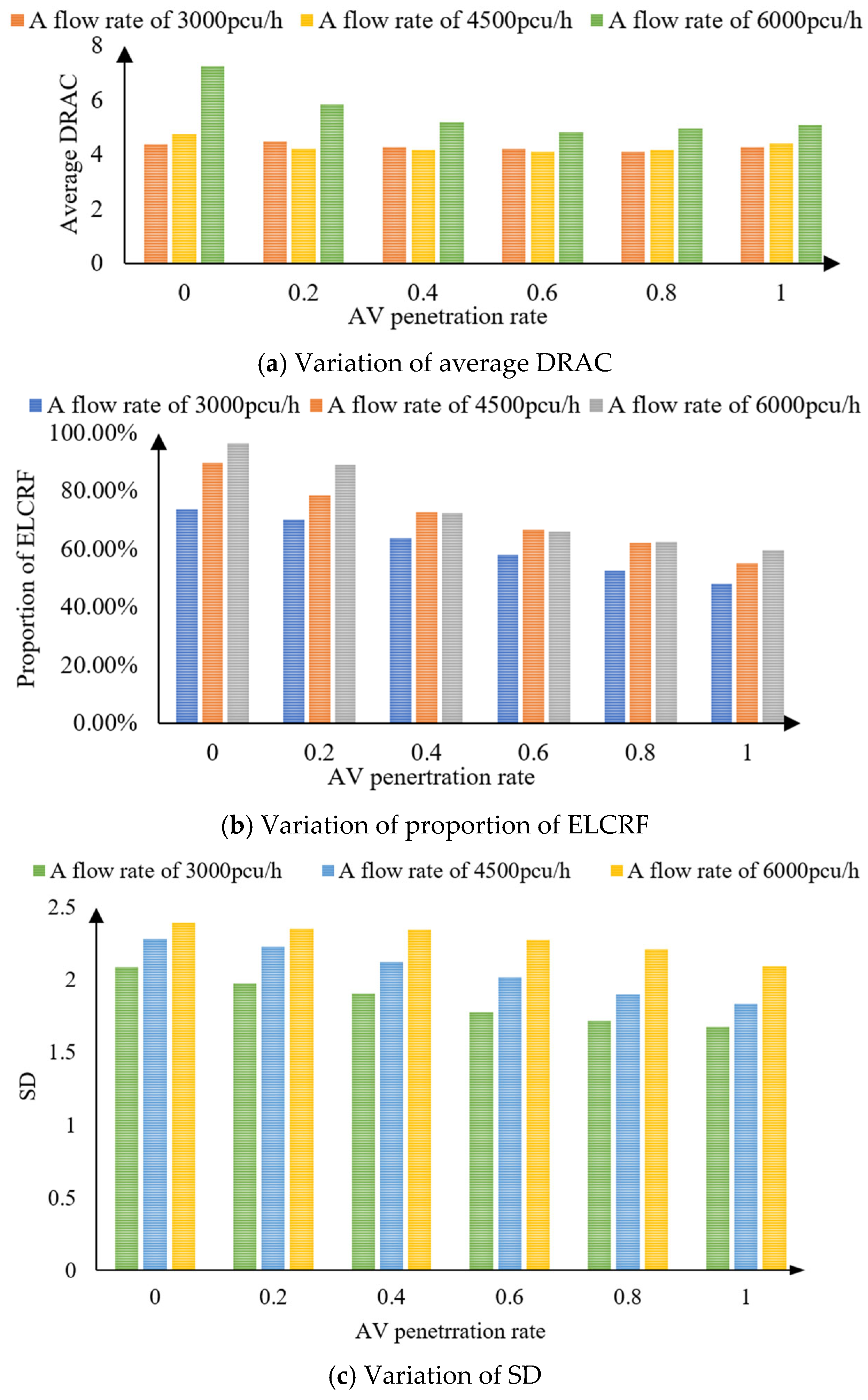
4.2.1. Temporal Dimension

Temporal Dimension indicators include headway, MTTC, and LCTTC. Figure 8 explores how these indicators change with varying AV penetration rates under different flow rates for a ramp flow ratio of 0.15.

In general, HDVs typically maintain a headway of 2–3 s as a standard safety following distance [44]. In contrast, autonomous vehicles (AVs) can achieve shorter headways due to advanced sensing technologies and faster response capabilities, as confirmed by our simulation results. As shown in Figure 8a, when the following vehicle is an AV, the average headway of HDVs is primarily distributed between 2–3 s, while that of AVs is concentrated in the 1–2 s range. This pattern remains consistent across various traffic flow scenarios. Although AVs consistently maintain shorter headways compared to HDVs, both exhibit a general upward trend in headway with increasing AV penetration rates, likely due to the currently conservative driving behavior of AVs.

In the safety analysis, threshold values for MTTC and LCTTC are typically set at 1.5 s and 6 s, respectively [19,20]. As illustrated in Figure 8b, the frequency of potential collisions generally increases with the rise in AV penetration rate, except for a slight decrease at low and medium traffic volumes when the penetration rate increases from 0.4 to 0.8. This suggests that under light to moderate traffic conditions, AVs may not significantly reduce the risk of longitudinal conflicts. However, at higher traffic demands (6000 pcu/h), the frequency of MTTC events tends to decrease with increasing AV penetration, except in the scenario with 100% AVs.

Figure 8c shows that the frequency of LCTTC events initially increases and then decreases as AV penetration rises across all three traffic scenarios. This indicates that interactions between AVs and HDVs introduce greater risks at low AV penetration rates, which is consistent with findings from previous studies [40,45]. When AV penetration is low (less than 20%), HDVs dominate the traffic composition. The variability and unpredictability of human driving behavior results in more potential conflicts during lane-change maneuvers. As the AV proportion increases, coordinated and more predictable lane-changing behavior among AVs contributes to a reduction in the frequency of LCTTC events.

4.2.2. Spatial Dimension

Spatial dimension indicators include DRAC, ELCRF, and SD. Figure 9 exhibits how these indicators vary with AV penetration rate for a ramp flow ratio of 0.15.

Based on relevant literature [46] and the values of DRAC in the SUMO software (version 1.18), the threshold for DRAC is set at 3 m/s². A higher DRAC value indicates a greater level of deceleration required to avoid a collision, reflecting more hazardous traffic conditions where vehicles must apply more aggressive braking to ensure safety. As shown in Figure 9a, when AVs are initially introduced into the traffic stream at low penetration rates, DRAC values increase under low-flow conditions. This may be attributed to the dispersed nature of potential collision risks, requiring AVs to apply higher deceleration rates. However, as AV penetration increases, AVs begin to exhibit cooperative behavior. In the face of potential conflicts, AVs can anticipate and respond proactively, reducing the need for sharp deceleration. Consequently, DRAC values gradually decrease. In high-flow conditions, although the traffic environment becomes more challenging, the technical advantages of AVs—such as precise speed regulation and consistent gap maintenance—become more pronounced, resulting in a further reduction in DRAC values.

Figure 9b represents that the proportion of ELCRF is related to flow rate and AV penetration rate. Under high traffic flow conditions, the interference and conflict between vehicles are intensified, which leads to the increase of ELCRF in the merging area and a greater safety risk. But the proportion of ELCRF gradually decreases with the increase of AV penetration rate in each traffic scenario, which illustrates that AVs significantly reduce the likelihood of emergency lane changes because of their fast response capabilities and stable driving control. Take the low-traffic scenario as an example; in the early stages of mixed traffic, the decrease in ELCRF is relatively slow (4.8%), and the advantages of AVs are not yet apparent. However, as the AV penetration rate increases, the overall frequency of emergency lane changes shows a clear downward trend. When the AV penetration rate reaches 0.8, AVs have become the dominant force in traffic, and while the frequency of emergency lane changes continues to decrease, the rate of decrease slows down from 9.8% to 8.2%.

A similar trend is observed for the standard deviation of speed (SD), as shown in Figure 9c. SD increases with traffic flow volume due to more frequent vehicle interactions and conflicts, which introduce speed fluctuations. However, SD decreases as AV penetration rises. This reflects a transition from a disordered mixed-traffic system to a more coordinated and homogeneous flow. As AVs gradually dominate the traffic stream, their stable operational characteristics contribute to improved flow consistency and reduced speed variability, thereby enhancing overall traffic stability.

Based on the above analysis, AV technology demonstrates a generally positive effect on improving traffic safety, particularly in high-flow scenarios. Although each safety indicator provides valuable insights, individual metrics may offer biased or incomplete representations. For instance, while SD and ELCRF suggest consistent improvements with increasing AV penetration, indicators such as LCTTC and DRAC initially show a deterioration in safety before improving. Meanwhile, metrics like MTTC and headway exhibit no substantial changes. These discrepancies highlight the limitations of relying on a single indicator to assess traffic safety. To address this issue, the present study adopts a comprehensive evaluation approach, in which multiple indicators are integrated to complement and validate each other. This method allows for a more holistic and accurate assessment of compound traffic safety risks arising from diverse interacting factors across different traffic conditions.

4.3. Comprehensive Evaluation Result

4.3.1. Weights of Indicators

Based on the simulation results, the objective weights and subjective weights of the six evaluation indicators were calculated using the entropy method and the DEMATEL method, respectively, as described in Section 3.3. The objective weight vector is $w_j=\left[0.0761,0.0332,0.1370,0.1257,0.5751,0.0529\right]$ and the subjective weight vector is $w_{\mathrm{i}}=\left[0.1477,0.1887,0.1739,0.1820,0.1580,0.1497\right]$. Subsequently, the improved game theory approach was applied to integrate the two types of weights.

Since the study only involves two types of weight sources (objective and subjective), the derivation of the optimal combination coefficients can be simplified analytically. This simplification is based on the minimization of deviation between the integrated weight and the individual weights, which is conceptually aligned with the cosine angle method in vector analysis. This simplification enhances computational clarity and efficiency.

The optimal combination coefficient ${\beta }_1$ is computed as follows:

$${\beta }_1={\displaystyle \frac{{\displaystyle {\sum }_{i=1}^6{w}_j\cdot }{w}_i}{{\displaystyle {\sum }_{i=1}^6{w}_j^2+w_i^2}}}$$

(43)

$${\beta }_2=1-{\beta }_1$$

(44)

Substituting the values in Equation (43):

$${\displaystyle {\sum }_{i=1}^6{w}_j\cdot }{w}_i=0.01123+0.00627+0.02382+0.02288+0.09089+0.00792=0.16301$$

$${\displaystyle {\sum }_{i=1}^6{w}_j^2+w_i^2}=0.02760+0.03680+0.04899+0.04892+0.35568+0.02521=0.54320$$

Thus,

$${\beta }_1={\displaystyle \frac{0.16301}{0.54320}}\approx 0.3001,{\beta }_2=1-{\beta }_1=0.6999$$

The resulting combination coefficients for the objective and subjective weights were 0.3001 and 0.6999, respectively, indicating a greater contribution from the objective component. Finally, the comprehensive weights of the six indicators were determined and are presented in

Table 4. Comprehensive weights of six indicators.

Indicator	Objective Weight	Subjective Weight	Comprehensive Weight
SD	0.076119	0.1477	0.126219
MTTC	0.033229	0.1887	0.142044
Headway	0.136975	0.1739	0.162819
ELCRF	0.575076	0.1580	0.283162
LCTTC	0.125701	0.1497	0.165105
DRAC	0.052900	0.1820	0.120651

.

4.3.2. Safety Evaluation Based on Cloud Model

(1)

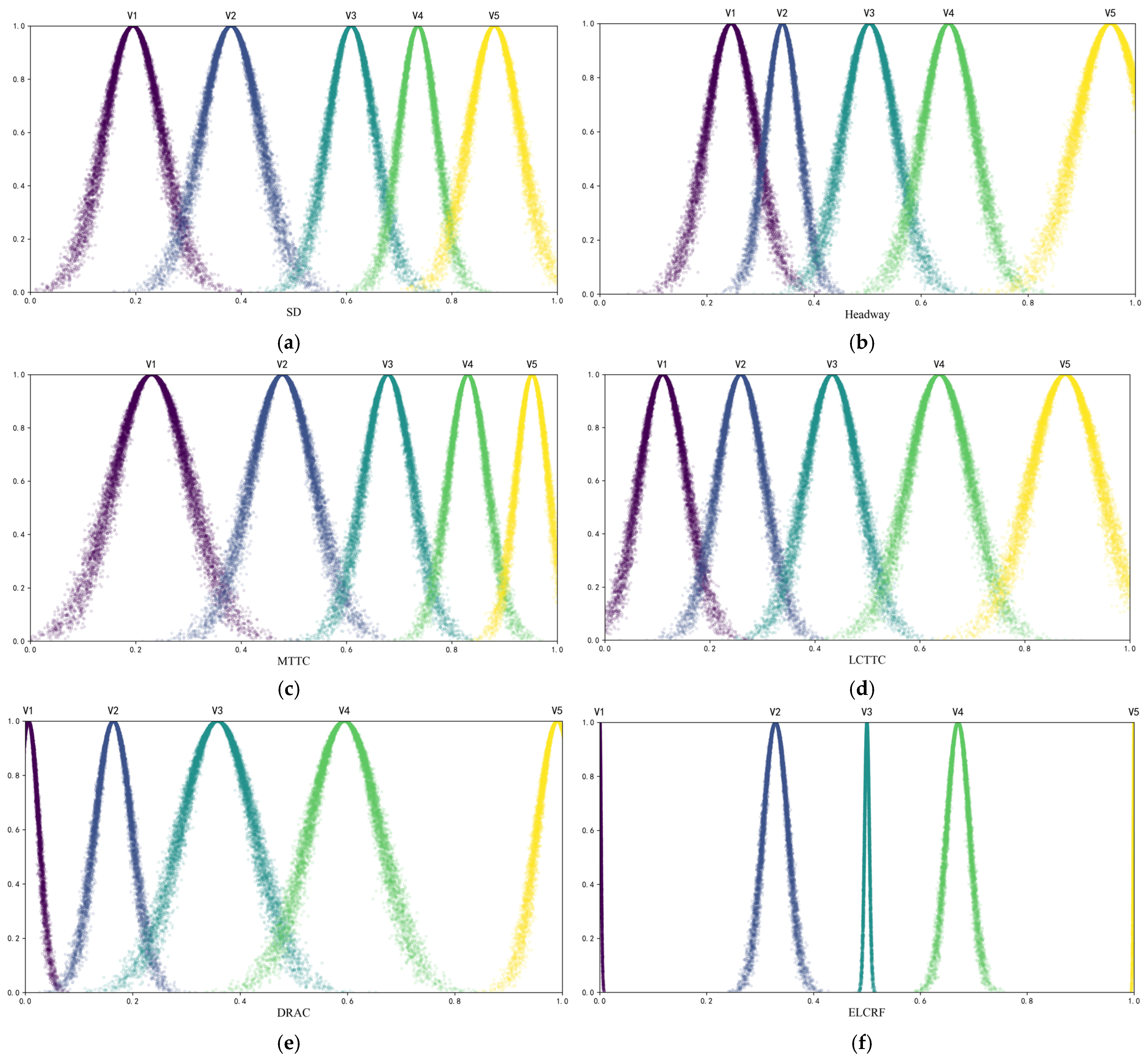
Determination of standard cloud parameters of indicators

Based on the cloud model theory and the Fuzzy C-Means (FCM) clustering method, the standard cloud parameters (i.e., expected value, entropy, and hyper-entropy) for each evaluation indicator were obtained. These parameters are summarized in

Table 5. Standard cloud parameters of indicators.

Index	High Risk	Moderate Risk	Average Risk	Low Risk	Very Low Risk
SD	(0.1946, 0.0550, 0.0055)	(0.3806, 0.0562, 0.0056)	(0.6088, 0.0454, 0.0045)	(0.7356, 0.0361, 0.0036)	(0.8806, 0.0493, 0.0049)
MTTC	(0.2300, 0.0721, 0.0072)	(0.4781, 0.0610, 0.0061)	(0.6785, 0.0469, 0.0047)	(0.8302, 0.0377, 0.0038)	(0.9522, 0.0309, 0.0031)
Headway	(0.2450, 0.0470, 0.0047)	(0.3408, 0.0319, 0.0032)	(0.5034, 0.0497, 0.0050)	(0.6514, 0.0497, 0.0050)	(0.9536, 0.0649, 0.0065)
ELCRF	(0.0000, 0.0024, 0.0002)	(0.3288, 0.0233, 0.0023)	(0.5000, 0.0044, 0.0004)	(0.6706, 0.0215, 0.0022)	(1.0000, 0.0016, 0.0002)
DRAC	(0.0059, 0.0195, 0.0020)	(0.1640, 0.0348, 0.0035)	(0.3580, 0.0685, 0.0068)	(0.5942, 0.0662, 0.0066)	(0.9908, 0.0376, 0.0038)
LCTTC	(0.1102, 0.0455, 0.0046)	(0.2587, 0.0454, 0.0045)	(0.4329, 0.0521, 0.0052)	(0.6368, 0.0605, 0.0061)	(0.8769, 0.0671, 0.0067)

. Furthermore, the corresponding standard cloud models for the six evaluation indicators were constructed and are illustrated in Figure 10, providing a visual representation of the distribution characteristics across different safety levels.

As an illustrative example, a simulation scenario (I2) with a total traffic flow rate of 6000 pcu/h, a ramp-to-mainline flow ratio of 0.35, and an AV penetration rate of 20% is selected. Based on this scenario, the cloud parameters of the six evaluation indicators are calculated and presented in

Table 6. Evaluation of indicators for cloud parameters.

Index	Evaluation Cloud Model
SD	(0.43782, 0.04932, 0.00493)
MTTC	(0.70533, 0.03085, 0.00309)
Headway	(0.35217, 0.06493, 0.00649)
ELCRF	(0.7799, 0.00157, 0.00016)
DRAC	(0.25507, 0.03762, 0.00376)
LCTTC	(0.36644, 0.06712, 0.00671)

. In addition, the evaluation cloud diagrams for each indicator under scenario I2 are visualized in Figure 11, providing insight into the distribution and membership characteristics of the safety evaluation results.

The comprehensive membership degree of the selected scenario can be calculated by Equations (41)–(43), and the result is shown in

Table 7. Comprehensive membership degree.

Level	High Risk	Moderate Risk	Average Risk	Low Risk	Very Low Risk
Membership degree	0.13783	0.29523	0.28214	0.2848	0

.

According to the principle of maximum membership degree, the safety of the selected traffic scenario is classified as level 2, indicating a moderate risk. Using the same method, the security risk levels of all 54 traffic scenarios are determined. The summarized results are shown in

Table 8. Safety levels of 54 simulation scenarios.

Scenarios	Level	Scenarios	Level	Scenarios	Level
3000/0.15/0.0	4	3000/0.25/0.0	4	3000/0.35/0.0	4
3000/0.15/0.2	2	3000/0.25/0.2	4	3000/0.35/0.2	3
3000/0.15/0.4	4	3000/0.25/0.4	4	3000/0.35/0.4	3
3000/0.15/0.6	3	3000/0.25/0.6	3	3000/0.35/0.6	3
3000/0.15/0.8	3	3000/0.25/0.8	4	3000/0.35/0.8	3
3000/0.15/1.0	3	3000/0.25/1.0	3	3000/0.35/1.0	2
4500/0.15/0.0	2	4500/0.25/0.0	4	4500/0.35/0.0	4
4500/0.15/0.2	2	4500/0.25/0.2	4	4500/0.35/0.2	4
4500/0.15/0.4	2	4500/0.25/0.4	3	4500/0.35/0.4	3
4500/0.15/0.6	4	4500/0.25/0.6	4	4500/0.35/0.6	3
4500/0.15/0.8	4	4500/0.25/0.8	4	4500/0.35/0.8	4
4500/0.15/1.0	4	4500/0.25/1.0	4	4500/0.35/1.0	4
6000/0.15/0.0	4	6000/0.25/0.0	4	6000/0.35/0.0	4
6000/0.15/0.2	2	6000/0.25/0.2	2	6000/0.35/0.2	2
6000/0.15/0.4	2	6000/0.25/0.4	3	6000/0.35/0.4	3
6000/0.15/0.6	4	6000/0.25/0.6	2	6000/0.35/0.6	3
6000/0.15/0.8	4	6000/0.25/0.8	3	6000/0.35/0.8	4
6000/0.15/1.0	4	6000/0.25/1.0	4	6000/0.35/1.0	4

, while the detailed numerical values of the safety evaluation indicators and corresponding risk levels for each scenario are provided in Appendix A for reference.

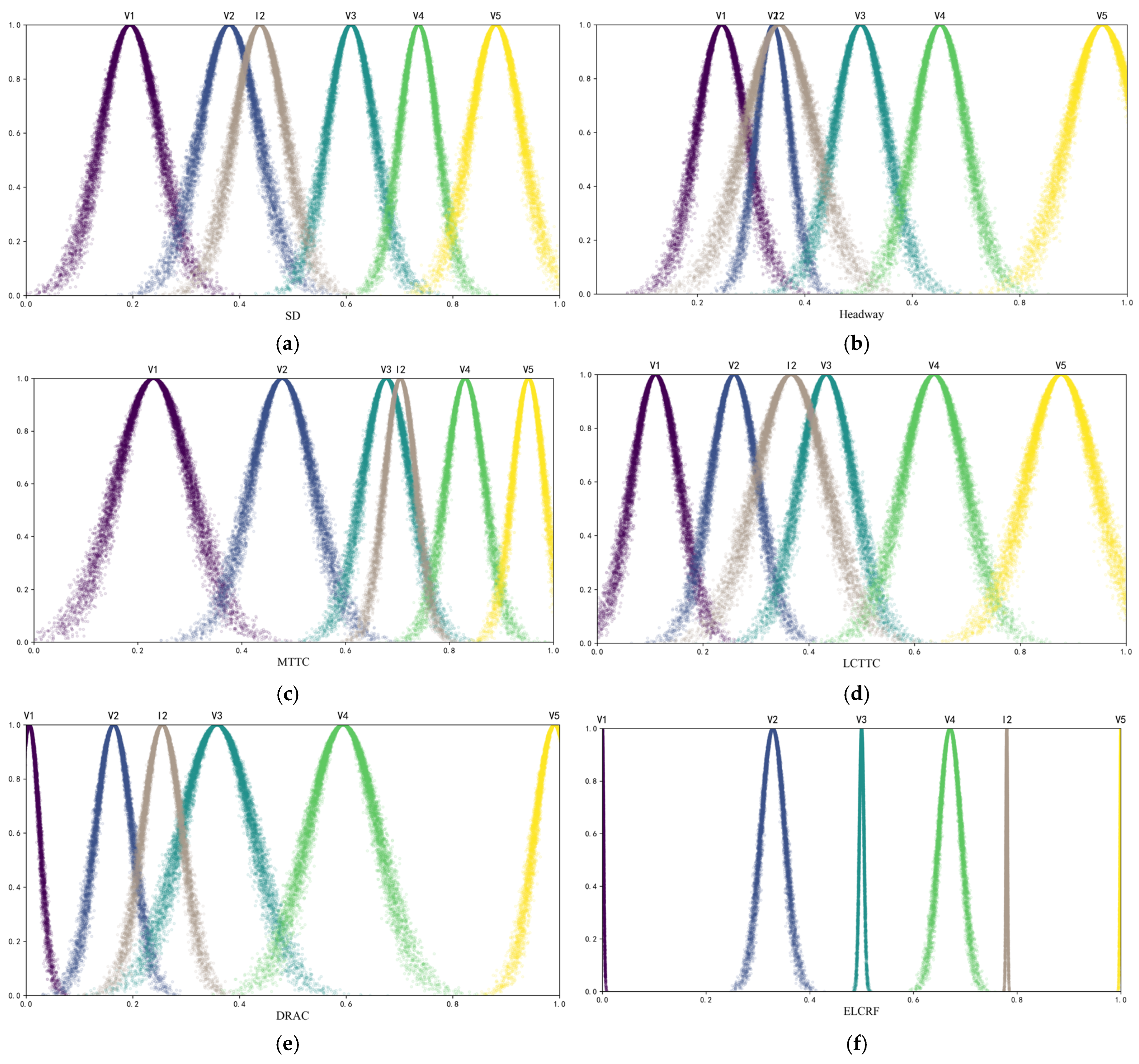
4.3.3. Validation of Cloud Model

To validate the rationality and reliability of the proposed cloud model, this study selected several simulation scenarios with a traffic flow rate of 6000 pcu/h and a ramp-to-mainline flow ratio of 0.15. These scenarios are evaluated and compared using the Fuzzy Comprehensive Evaluation (FCE) method. The comparison results between the cloud model and the FCE method are presented in

Table 9. Comparison results.

Method	Scenarios	High Risk	Moderate Risk	Average Risk	Low Risk	Very Low Risk	FCM Method
FCM method	6000/0.15/0.0	0	0.28273	0.33944	0.18135	0.19648	average risk
Cloud model		0.01047	0.38381	0.03276	0.57277	0.00019	low risk
FCM method	6000/0.15/0.2	0	0.41587	0.27713	0.09430	0.21270	moderate risk
Cloud model		0.02237	0.53419	0.01905	0.42259	0.00181	moderate risk
FCM method	6000/0.15/0.4	0	0.36460	0.36382	0.17739	0.09418	moderate risk
Cloud model		0.02931	0.51709	0.08923	0.36436	0	moderate risk
FCM method	6000/0.15/0.6	0	0.37520	0.26329	0.28351	0.07799	moderate risk
Cloud model		0.02577	0.25683	0.28684	0.43051	0.00005	low risk
FCM method	6000/0.15/0.8	0.12807	0.30368	0.16393	0.40432	0	low risk
Cloud model		0.13423	0.14492	0.19867	0.51818	0.00401	low risk
FCM method	6000/0.15/1.0	0.28300	0.10035	0.27155	0.31174	0.03336	low risk
Cloud model		0.12749	0.12628	0.33425	0.35687	0.0551	low risk

, demonstrating the consistency and effectiveness of the cloud-based safety evaluation approach.

According to Table 9, when the penetration rates of autonomous vehicles (AVs) are 0.2, 0.4, 0.8, and 1.0, the evaluation results of both the fuzzy comprehensive evaluation (FCE) method and the cloud model show the same overall trend, indicating the reliability of the cloud model in traffic safety evaluation. In the scenario of 6000/0.15/0.2, both methods predict moderate risk. At this stage, a small number of autonomous vehicles in the mixed traffic flow may cause some disruption, and the cloud model (0.53419) shows a more precise distribution compared to FCE (0.41587), reflecting its ability to capture subtle safety differences. When the AV penetration rate reaches 0.6, the road transitions to an AV-dominated flow where the FCE method still classifies the risk as moderate while the cloud model classifies it as low risk, showing more accurate results and better reflecting the safety improvements brought by AVs. Overall, the cloud model adapts better to higher AV penetration rates and provides a more accurate reflection of real-world traffic conditions, especially in mixed traffic environments.

4.3.4. Results Analysis

Based on the evaluation results presented in Table 7, it is evident that autonomous vehicle (AV) technologies can effectively reduce traffic safety risks. From the perspective of traffic flow rate, scenarios with lower traffic volumes exhibit significantly higher safety levels than those with higher flow rates, reflecting a more symmetrical traffic environment where interactions between vehicles are less complex. In merging areas with higher traffic flow, it may be beneficial to establish dedicated lanes for AVs and use intelligent transportation systems (ITS) to dynamically monitor vehicle statuses and adjust speed limit and acceleration lanes in real-time based on traffic flow conditions. From the perspective of a ramp-to-mainline flow ratio, taking an AV penetration rate of 0.6 as an example, at a low traffic flow rate (3000 pcu/h), the increase in ramp flow ratio does not significantly affect the safety risk level, which remains at the “moderate” level across all cases. However, at higher flow rates, increasing the ramp flow ratio leads to a clear decrease in safety level, indicating that greater merging pressure under congestion conditions contributes to elevated traffic risk. The asymmetry introduced by the ramp flow ratio imbalance creates unpredictable merging behaviors and worsens safety, especially in mixed traffic conditions. Under high traffic flow conditions, ITS can be used to adjust ramp flow ratios in real-time to ensure the merging pressure between the ramp and mainline is effectively distributed, avoiding excessive congestion that could negatively impact safety.

As the AV penetration rate increases, the overall safety level improves, particularly under high traffic demand conditions, shifting the system towards more symmetric traffic behavior, where the interactions between AVs and HDVs become more predictable and coordinated. At low (3000 pcu/h) and moderate (4500 pcu/h) traffic flow rates, the evaluated safety levels are mostly concentrated in the categories of “low risk” and “average risk”, suggesting that the advantages of AVs are not fully realized in smoother traffic conditions. This may be attributed to the conservative behavior of AVs, which could lead to suboptimal interactions and even potential conflicts. In addition, when the AV penetration rate increases from 0 to 0.2, a drop in safety level is observed. This implies that interactions between AVs and human-driven vehicles (HDVs) at low AV penetration rates may introduce instability and increase risk—an outcome that aligns with findings from previous studies [45]. At this stage, the asymmetry is heightened as human-driven vehicles dominate the traffic flow, leading to unpredictable interactions and higher safety risks. Although the overall evaluation results are reasonable and align with actual traffic conditions, there are still some scenarios where the outcomes seem unreasonable. For instance, in a scenario with a flow rate of 3000 pcu/h, a ramp flow ratio of 0.35, and an AV penetration rate of 1.0, the safety level is classified as a “moderate risk”. This inconsistency may arise from the inherent deviations in the simulation data compared to real-world conditions. Additionally, the thresholds selected for certain indicators might not be fully applicable to a fully autonomous driving environment where AVs would dominate the traffic and lead to more symmetric interactions. Therefore, with the continued development of AV technology, it is essential to recalibrate the results using real-world mixed traffic data and further refine the indicators and their thresholds to better capture the asymmetries and symmetries inherent in mixed traffic environments.

With the rapid development of autonomous driving technology, the mixed traffic scenario of autonomous and human-driven vehicles will become the norm in the near future. It is essential to improve safety in merging areas under such conditions. Based on our research findings, the following suggestions are proposed to improve the safety of mixed traffic flow in the merging area: (1) Variable speed limit signs can be installed upstream of merging zones to reduce speed differentials and traffic flow on the main line to reduce conflicts. Moreover, ramp metering or lane-specific traffic signals are implemented to regulate HDV merging flow and enforce zipper merging. (2) Penetration-based strategies are adopted. When AV penetration rate is less than 0.2, AVs are allowed to proactively accelerate for merging to prevent AVs’ conservative behavior from triggering frequent HDV lane changes or conflicts. when AV penetration rate is between 0.2 and 0.8, V2X coordination and dynamic lane allocation are used to facilitate HDV-AV coordination to reduce conflicts from behavioral differences. When AV penetration rate is more than 0.8, measures such as platooning and centralized scheduling are taken to maximize AV coordination potential to boost overall traffic safety and efficiency. (3) The government should speed up the formulation of relevant legislation on automatic driving vehicles, clarify the division of responsibilities, and provide a solid legal and policy guarantee for mixed traffic environment.

5. Conclusions

Autonomous vehicle (AV) technologies hold significant promise for improving traffic safety. However, the asymmetric interactions between AVs and human-driven vehicles (HDVs) in mixed traffic conditions—especially in freeway merging areas—introduce new safety challenges due to complex lane-changing maneuvers. This study proposed a comprehensive traffic safety evaluation framework for such scenarios by integrating Surrogate Safety Measures (SSMs) with a cloud model enhanced by Fuzzy C-Means (FCM) clustering. The key conclusions are as follows:

(1)

A novel indicator—Emergency Lane-Change Risk Frequency (ELCRF)—was developed to better capture the frequency and severity of urgent lane-changing behavior in merging areas. Together with five other SSM-based indicators, this metric contributes to a multi-dimensional safety evaluation system spanning temporal, spatial, macro, and micro perspectives.

(2)

A comprehensive safety evaluation model was developed by combining FCM with the cloud model. In addition, a modified game theory was employed to balance the objective weight and subjective weight of indexes, which effectively handles differences between expert judgment and data-driven results. Through a comparative case study with the fuzzy comprehensive evaluation (FCE) method, the results demonstrated that the modified cloud model is both feasible and better aligned with actual traffic dynamics.

(3)

Simulation results across various traffic scenarios indicated that increasing AV penetration rates generally lead to improved safety levels, especially under high traffic volumes. However, low AV penetration rates (less than 20%) introduce greater asymmetry, leading to unstable interactions between AVs and HDVs, which deteriorates safety. This conclusion provides valuable insight for the government to formulate the development policy of AV. Overall, the increase of flow rate and ramp flow ratio also will worsen traffic safety of mixed traffic. Therefore, necessary flow control measures under high flow and ramp flow ratio, such as ramp flow restriction and variable speed limited strategy, are very important to improve the safety of mixed traffic flow in merging areas.

(4)

Some valuable suggestions were put forward based on our findings, such as penetration-based strategies, flow control, V2X coordination technology, and improvement of the legal framework.

The proposed methodology is generic and applicable to various traffic scenarios, such as intersections, diverging zones, or arterial roads. The selection of appropriate evaluation indicators and the calibration of model parameters may vary depending on the specific conflict types and traffic dynamics in these scenarios. In this study, we focus on freeway merging areas as a representative case. While the current work demonstrates the applicability of the method in one specific context, it also has some limitations that future research should address: (1) The simulation model parameters used in this study are mainly obtained from the previous literature, which may lead to a deviation between simulation results and practical scenarios. Future studies should focus on calibrating the simulation model with real-world traffic data. Notably, autonomous vehicles such as Robotaxi are already in regular operation on public roads in Wuhan, China. Our research team plans to capture aerial traffic videos in freeway merging areas using drones. The collected videos will be processed with the YOLO object detection algorithm to identify individual vehicles, and DeepSORT will be applied to continuously track their trajectories. The resulting trajectory data will be used to support parameter calibration and model validation, thereby enhancing the realism and applicability of the simulation model in mixed traffic scenarios. (2) The selection of evaluation indicators mainly focused on traffic flow characteristics and conflict metrics. In future work, additional factors such as road geometry, driving behavior, and environmental conditions should be incorporated to build a more comprehensive safety evaluation framework. (3) This study only focused on a single type of freeway merging area with a single-lane parallel acceleration lane. However, different types of merging configurations (e.g., taper merging, two-lane on-ramps) may affect the safety level of mixed traffic flow. Hence, exploring different merging configurations should be paid attention to in future. (4) The validation of the proposed model was based on a qualitative comparison with the traditional fuzzy comprehensive evaluation (FCE) method. Although both models showed consistent trends and the cloud model exhibited greater sensitivity in risk differentiation, the validation lacked formal statistical measures. Future research should incorporate quantitative metrics such as root mean square error (RMSE), correlation analysis, or other statistical validation techniques to improve the model’s robustness and ensure its accuracy and reliability under various traffic scenarios.

References

1. Mergia, W.Y.; Eustace, D.; Chimba, D.; Qumsiyeh, M. Exploring factors contributing to injury severity at freeway merging and diverging locations in Ohio. Accid. Anal. Prev. 2013, 55, 202–210. [Google Scholar] [CrossRef] [PubMed]
2. Yu, Q.; Lei, L.; Bao, Y.; Wang, L. Research on safety and traffic efficiency of mixed traffic flows in the converging section of a super-freeway ramp. Sustainability 2022, 14, 13234. [Google Scholar] [CrossRef]
3. Chen, P.; Ni, H.; Wang, L.; Yu, G.; Sun, J. Safety performance evaluation of freeway merging areas under autonomous vehicles environment using a co-simulation platform. Accid. Anal. Prev. 2024, 199, 107530. [Google Scholar] [CrossRef] [PubMed]
4. Abdel-Aty, M.; Ding, S. A matched case-control analysis of autonomous vs human-driven vehicle accidents. Nat. Commun. 2024, 15, 4931. [Google Scholar] [CrossRef]
5. Li, T.; Han, X.; Ma, J.; Ramos, M.; Lee, C. Operational safety of automated and human driving in mixed traffic environments: A perspective of car-following behavior. Proc. Inst. Mech. Eng. Part O J. Risk Reliab. 2023, 237, 355–366. [Google Scholar] [CrossRef]
6. Ma, Z.; Zhang, Y. Driver-automated vehicle interaction in mixed traffic: Types of interaction and drivers’ driving styles. Hum. Factors J. Hum. Factors Ergon. Soc. 2024, 66, 544–561. [Google Scholar] [CrossRef]
7. Zhu, J.; Gao, K.; Li, H.; He, Z.; Monreal, C.O. Bi-level ramp merging coordination for dense mixed traffic conditions. Fundam. Res. 2024, 4, 992–1008. [Google Scholar] [CrossRef]
8. Zhu, J.; Ma, Y.; Lou, Y. Multi-vehicle interaction safety of connected automated vehicles in merging area: A real-time risk assessment approach. Accid. Anal. Prev. 2022, 166, 106546. [Google Scholar] [CrossRef]
9. Morando, M.M.; Tian, Q.; Truong, L.T.; Vu, H.L. Studying the safety impact of autonomous vehicles using simulation-based surrogate safety measures. J. Adv. Transp. 2018, 2018, 6135183. [Google Scholar] [CrossRef]
10. Papadoulis, A.; Imprialou, M.; Feng, Y.; Quddus, M. Simulating and modelling the safety impact of connected and autonomous vehicles in mixed traffic: Platoon size, sensor error, and path choice. Machines 2024, 12, 371. [Google Scholar] [CrossRef]
11. Fu, C.; Sayed, T. Multivariate Bayesian hierarchical Gaussian copula modeling of the non-stationary traffic conflict extremes for crash estimation. Anal. Methods Accid. Res. 2021, 29, 100154. [Google Scholar] [CrossRef]
12. Sinha, A.; Chand, S.; Wijayaratna, K.P.; Virdi, N.; Dixit, V. Comprehensive safety assessment in mixed fleets with connected and automated vehicles: A crash severity and rate evaluation of conventional vehicles. Accid. Anal. Prev. 2020, 142, 105567. [Google Scholar] [CrossRef] [PubMed]
13. Wang, C.; Xie, Y.; Huang, H.; Liu, P. A review of surrogate safety measures and their applications in connected and automated vehicles safety modeling. Accid. Anal. Prev. 2021, 157, 106157. [Google Scholar] [CrossRef] [PubMed]
14. Behbahani, H.; Hosseini, S.M.; Taherkhani, A.; Asadi, H.; Samerei, S.A. Proposing new methods to estimate the safety level in different parts of freeway interchanges. Adv. Civ. Eng. 2018, 2018, 8702854. [Google Scholar] [CrossRef]
15. Zhu, J.; Tasic, I. Safety analysis of freeway on-ramp merging with the presence of autonomous vehicles. Accid. Anal. Prev. 2021, 152, 105966. [Google Scholar] [CrossRef]
16. Wang, C.; Xu, C.; Xia, J.; Qian, Z.; Lu, L. A combined use of microscopic traffic simulation and extreme value methods for traffic safety evaluation. Transp. Res. Part C Emerg. Technol. 2018, 90, 281–291. [Google Scholar] [CrossRef]
17. Yao, Z.; Hu, R.; Jiang, Y.; Xu, T. Stability and safety evaluation of mixed traffic flow with connected automated vehicles on expressways. J. Saf. Res. 2020, 75, 262–274. [Google Scholar] [CrossRef]
18. Jiang, Y.; Ren, T.; Ma, Y.; Wu, Y.; Yao, Z. Traffic safety evaluation of mixed traffic flow considering the maximum platoon size of connected automated vehicles. Phys. A Stat. Mech. Its Appl. 2023, 612, 128452. [Google Scholar] [CrossRef]
19. Garg, M.; Bouroche, M. Can connected autonomous vehicles improve mixed traffic safety without compromising efficiency in realistic scenarios? IEEE Trans. Intell. Transp. Syst. 2023, 24, 6674–6689. [Google Scholar] [CrossRef]
20. He, Y.; Kong, Y. Traffic impact analysis of expressway accident in mixed traffic environment of connected and autonomous considering multi-factor coupling. IEEE Access 2025, 13, 57342–57353. [Google Scholar] [CrossRef]
21. Hu, X.; Huang, M.; Guo, J. Feature analysis on mixed traffic flow of manually driven and autonomous vehicles based on cellular automata. Math. Probl. Eng. 2020, 2020, 7210547. [Google Scholar] [CrossRef]
22. Kong, D.; Sun, L.; Chen, Y. Traffic dynamics around freeway merging area with mixed conventional vehicles and connected and autonomous vehicles. Int. J. Mod. Phys. C 2022, 33, 2250128. [Google Scholar] [CrossRef]
23. Zhu, L.; Lu, L.; Wang, X.; Jiang, C.; Ye, N. Operational characteristics of mixed-autonomy traffic flow on the freeway with on- and off-ramps and weaving sections: An rl-based approach. IEEE Trans. Intell. Transp. Syst. 2021, 23, 13512–13525. [Google Scholar] [CrossRef]
24. Das, T.; Samandar, M.S.; Rouphail, N. Longitudinal traffic conflict analysis of autonomous and traditional vehicle platoons in field tests via surrogate safety measures. Accid. Anal. Prev. 2022, 177, 106822. [Google Scholar] [CrossRef]
25. Zheng, L.; Ismail, K.; Sayed, T.; Fatema, T. Bivariate extreme value modeling for road safety estimation. Accid. Anal. Prev. 2018, 120, 83–91. [Google Scholar] [CrossRef]
26. Wu, H. Safety Evaluation of Railway Passenger Transport Based on Improved CRITIC Cloud Model. Railw. Transp. Econ. 2024, 46, 207–214+222. [Google Scholar]
27. Liu, H.; He, Y. Comprehensive Evaluation of Resilience for Qinling Tunnel Group Operation Safety System Based on Combined Weighting and Cloud Model. Sustainability 2024, 16, 3937. [Google Scholar] [CrossRef]
28. Vuong, X.C.; Mou, R.F.; Vu, T.T.; Tran, V.H.; Nguyen, C.T. A safety evaluation model of intersections under mixed traffic conditions using traffic conflicts and cloud model. J. Adv. Transp. 2021, 2021, 5899673. [Google Scholar] [CrossRef]
29. Sharma, A. Analyzing Crash Potential in Mixed Traffic with Autonomous and Human-Driven Vehicles. Master’s Thesis, Texas A&M University, San Antonio, TX, USA, 2019. [Google Scholar]
30. Cheng, G.; Meng, F.; Lv, J.; Chen, Y.; Xi, C. Dynamic Zonal Modeling and Connectivity: Enhancing Safety and Efficiency in Merging Zones. Phys. A Stat. Mech. Appl. 2025, 664, 130470. [Google Scholar] [CrossRef]
31. Arun, A.; Haque, M.; Washington, S.; Sayed, T.; Mannering, F. How many are enough?: Investigating the effectiveness of multiple conflict indicators for crash frequency-by-severity estimation by automated traffic conflict analysis. Transp. Res. Part C Emerg. Technol. 2022, 138, 103653. [Google Scholar] [CrossRef]
32. Ramezanı-khansarı, E.; Nejad, F.M.; Moogeh, S. Comparing time to collision and time headway as safety criteria. Pamukkale Univ. J. Eng. Sci. 2020, 27, 669–675. [Google Scholar] [CrossRef]
33. Amirgholy, M.; Yang, J.J. Decision Making and Policy Analysis in Transportation Planning; MDPI: Basel, Switzerland, 2024. [Google Scholar]
34. Dong, G.; Chen, C.; Xia, H. Safety Evaluation of Road Passenger Transportation Process by Fuzzy Comprehensive Evaluation Method and Entropy Value Method. In Recent Developments in Mechatronics and Intelligent Robotics; Springer: Singapore, 2020; pp. 671–678. [Google Scholar]
35. Ortíz, M.A.; Cómbita, J.P.; De la Hoz, Á.A.; De Felice, F.; Petrillo, A. An integrated approach of AHP-DEMATEL methods applied for the selection of allied hospitals in outpatient service. Int. J. Med. Eng. Inform. 2016, 8, 87. [Google Scholar] [CrossRef]
36. Wang, M.; Wang, Y.; Shen, F.; Jin, J. A novel classification approach based on integrated connection cloud model and game theory. Commun. Nonlinear Sci. Numer. Simul. 2021, 93, 105540. [Google Scholar] [CrossRef]
37. Nayak, J.; Naik, B.; Behera, H.S. Fuzzy C-means (FCM) clustering algorithm: A decade review from 2000 to 2014. In Computational Intelligence in Data Mining—Volume 2: Proceedings of the International Conference on CIDM, 20–21 December 2014; Springer: New Delhi, India, 2015; pp. 133–149. [Google Scholar]
38. Zeng, Y.; Wu, B.; Tian, N. Risk Assessment of Power Monitoring System Based on Cloud Model and Improved Evidence Theory. Comput. Syst. Appl. 2022, 31, 55–63. [Google Scholar]
39. CJJ37-2012; Design Code for Urban Expressways. Ministry of Housing and Urban-Rural Development of the People’s Republic of China: Beijing, China, 2016.
40. He, Y.; Xiang, D.; Wang, D. Traffic safety evaluation of emerging mixed traffic flow at freeway merging area considering driving behavior. Sci. Rep. 2025, 15, 10686. [Google Scholar] [CrossRef]
41. Pang, M.S. Analysis and Control of Traffic Flow in the Connected Autonomous Driving Environment. Master’s Thesis, Shanghai Institute of Technology, Shanghai, China, 2023. [Google Scholar]
42. Pelizza, A.; Orsini, F.; Yilmaz-Niewerth, S.; Rossi, R.; Friedrich, B. Exploring the impact of automated vehicles lane-changing behavior on urban network efficiency. In Proceedings of the 2023 8th International Conference on Models and Technologies for Intelligent Transportation Systems (MT-ITS), Nice, France, 14–16 June 2023; pp. 1–6. [Google Scholar]
43. Mintsis, E.; Koutras, D.; Porfyri, K.; Mitsakis, E.; Lücken, L.; Erdmann, J.; Flötteröd, Y.; Alms, R.; Rondinone, M.; Maerivoet, S.; et al. TransAID Deliverable 3.1—Modelling, Simulation and Assessment of Vehicle Automations and Automated Vehicles’ Driver Behaviour in Mixed Traffic—Iteration 2. Available online: https://elib.dlr.de/132647/ (accessed on 12 December 2019).
44. Ding, Z.; Wu, H.; Sun, Y. Research on Time Headway Mixture Distribution Model Based on YOLOv5 + DeepSORT Detection Data. Meas. Control. Technol. 2023, 42, 56–64. [Google Scholar]
45. Ma, Q.L.; Fu, B.Y.; Zeng, H.W. Fundamental diagram and stability analysis of heterogeneous traffic flow in a connected and autonomous environment. J. Transp. Inf. Saf. 2021, 39, 76–84. [Google Scholar]
46. Lee, H.; Park, S.H.; Kang, M. A safety analysis based on evaluation indicators of mixed traffic flow. J. Korea Inst. Intell. Transp. Syst. 2024, 23, 42–60. [Google Scholar] [CrossRef]
Figure 1. Schematic diagram of the merging area with a single-lane parallel-type acceleration lane.
Symmetry 17 00855 g001
Figure 2. Traffic safety evaluation framework.
Symmetry 17 00855 g002
Figure 3. Schematic diagram of MTTC.
Symmetry 17 00855 g003
Figure 4. Schematic diagram of LCTTC.
Symmetry 17 00855 g004
Figure 5. Schematic diagram of DRAC.
Symmetry 17 00855 g005
Figure 6. Schematic diagram of ELCRF.
Symmetry 17 00855 g006
Figure 7. Simulation scenario.
Symmetry 17 00855 g007
Figure 8. Analysis of spatial dimension indicators.
Symmetry 17 00855 g008
Figure 9. Analysis of time dimension indicators.
Symmetry 17 00855 g009
Figure 10. Calculation of cloud parameters of indicators. (a) Cloud model for SD; (b) cloud model for Headway; (c) cloud model for MTTC; (d) cloud model for LCTTC; (e) cloud model for DRAC; (f) cloud model for ELCRF.
Symmetry 17 00855 g010
Figure 11. Determination of safety level. (a) Evaluation cloud for SD; (b) evaluation cloud for Headway; (c) evaluation cloud for MTTC; (d) evaluation cloud for LCTTC; (e) evaluation cloud for DRAC; (f) evaluation cloud for ELCRF.
Symmetry 17 00855 g011