Abstract
Existing trajectory planning methods often face challenges in ensuring stable robot motion control, leading to significant positional errors during navigation. This study proposes Timed-Elastic-Band-Based Variable Splitting (TEB-VS), a novel framework that integrates variable splitting (VS)—a constrained optimization technique—with the classical Timed-Elastic-Band (TEB) algorithm. Unlike incremental modifications to TEB, TEB-VS introduces a systematic combination of VS and TEB to decompose non-convex global constraints into tractable subproblems while leveraging symmetry principles for balanced multi-objective control (e.g., velocity, acceleration, and obstacle avoidance). Experimental results demonstrate that TEB-VS achieves a improvement in motion stability over traditional TEB in obstacle-free simulations and a enhancement in dynamic obstacle scenarios. Real-world tests show a reduction in angular velocity oscillations, with computational efficiency comparable to TEB. The framework’s effectiveness in harmonizing trajectory smoothness and dynamic adaptability is validated through extensive simulations and TurtleBot2 experiments.
1. Introduction
With the continuous advancement of machine learning technologies, various autonomous systems are becoming integral parts of daily human life, including autonomous driving vehicles, unmanned aerial vehicles, and underwater robots, among others [1,2]. These systems contribute significantly to enhancing the efficiency of human activities, prompting extensive efforts to explore novel practical applications for autonomous technologies [3,4].
The traditional planning module in autonomous systems adopts a hierarchical structure, after map building with Simultaneous Localization and Mapping (SLAM) [5] or visual simultaneous localization and mapping (VSLAM) [6], featuring both a global planner and a local planner. The global planner accumulates environmental information and provides a globally optimal path, typically at a slower frequency. In contrast, the local planner is responsible for quickly searching for an optimal trajectory that adheres to the global path [7]. The well-known global planning method Dijkstra’s algorithm [8] is another popular pathfinding algorithm that combines the advantages of Dijkstra’s algorithm and greedy best-first search. It uses a heuristic to guide the search process towards the goal node, resulting in efficient pathfinding in many cases. The Jump Point Search algorithm [9] is an enhancement of the A* algorithm that incorporates jump point search (JPS) to accelerate the search process by skipping unnecessary nodes. It is particularly effective in grid-based environments with obstacles. A* algorithm [10] and the Jump Point Search algorithm [9]. It is particularly effective in grid-based environments with obstacles.
Researchers have proposed various methods to enhance the performance of trajectory planning algorithms, particularly based on the Dynamic Window Approach (DWA) [11] and Timed-Elastic-Band (TEB) [12] algorithms. In terms of local planning, both TEB and DWA algorithms can conceptualize the path planning problem as a multi-objective optimization problem. However, it turns out that, when applied to non-convex optimization problems, the methods will remain computationally expensive. Examples of these enhanced approaches include the Improved Dynamic Window Approach (IDWA) introduced in [13], which enhances the DWA by incorporating speed smoothing parameters and pedestrian avoidance parameters. By considering these additional factors, IDWA generates smoother and safer planned trajectories compared to traditional methods. The egoTEB method presented in [14] addresses the mismatch problem between grid-based representations and optimization graphs commonly encountered in TEB. By utilizing factor graphs, egoTEB offers improved optimization capabilities and better integration with grid-based representations, resulting in more accurate and efficient trajectory planning. At present, with the development of machine learning and reinforcement learning, many researchers will also use such methods in trajectory planning. Specifically, the method in [15] was based on an obstacle avoidance algorithm based on inverse reinforcement learning. The paper [16] introduced an algorithm based on deep learning and quadratic optimization, with the goal of enhancing the efficiency and success rate of trajectory planning. It appears that one of the challenges is the difficulty in addressing the robot swing in the path, and the existing methods are not effectively mitigating this issue.
Variable splitting (VS) methods play a crucial role in solving constrained optimization problems efficiently [17,18]. Among these algorithms, methods like Douglas–Rachford splitting (DRS) [19,20], Peaceman–Rachford splitting (PRS) [21,22], the first-order primal–dual (FOPD) method [23,24], and the alternating direction method of multipliers (ADMM) [4,25] are prominent. They leverage vs. techniques and are well suited for various linear/nonlinear constrained optimization problems. The basic principle of VS methods is to split the big optimization problems into several smaller subproblems by introducing several variables [17]. These methods can transform the objective problems with inequality constraints into equivalent ones with equality constraints, facilitating their resolution. Due to the nonlinearity of the objective function, the direct computation on such subproblems is highly expensive [15,26].
In scenarios involving inequality constraints, computing the solution to objective problems directly can be challenging. Heuristic optimization algorithms, while useful, have their limitations. These include susceptibility to local optima, the ineffective handling of constraints, and potential feasibility issues in high-dimensional settings. For instance, the Genetic Algorithm (GA) [27] mimics natural evolution to search for optimal solutions, offering robustness and optimization capability, but does not guarantee global optimal convergence. Simulated annealing [28] can address various combinatorial and continuous optimization problems but suffers from slow convergence and complex parameter tuning. The moth swarm algorithm [29] boasts a simple structure, fewer parameters, high accuracy, and robustness, making it adept at complex optimization problems. However, it is prone to local optima.
When addressing problems with a single objective function, such as finding an optimal solution, employing a nonlinear optimization method suffices. However, in the context of robot motion navigation, objectives are often multi-dimensional, involving various constraints like target path, speed, time, acceleration, and obstacle distance. Achieving overall optimization across these multiple objectives requires more sophisticated approaches. Graph optimization algorithms, like the Kuhn–Munkres algorithm [30], are well suited to solving multi-objective optimization problems. For instance, the problem of the two-way distribution of passengers and drivers on taxi platforms can be framed as a binary graph problem [31], making it suitable for such algorithms. In the realm of path-planning algorithms, the concept of incorporating graph optimization has been proposed. For example, the TEB algorithm adopts a weighted optimal matching method, seeking to find matches that maximize the sum of the weights of the matching edges. This integration of graph optimization enhances the algorithm’s capability of navigating complex environments effectively.
Graph optimization is a powerful technique commonly applied to SLAM and robot trajectory planning problems. It involves converting traditional optimization problems into graph-based representations, which are then solved using graph theory-based algorithms. One widely used graph optimization library is General Graph Optimization (G2O) [32]. The typical optimization process involves the following several key steps. The first is to define the types of nodes and edges needed in the graph and specify their parameterized forms. Then, we can populate the graph with actual nodes and edges representing the problem’s components. After that, we choose initial values for the parameters and start the iteration process. We then calculate the Jacobian matrix and Hessian matrix corresponding to the current parameter estimates and solve the sparse linear equations to obtain the gradient direction in each iteration. The last step is to iterate using either the Gauss–Newton (GN) method [33] or the Levenberg–Marquardt (LM) method [34]. These methods adjust the parameter estimates in the direction of the steepest descent until convergence is achieved. Once the iteration converges, the program can return the optimized parameter values.
Many researchers have explored optimizations for the TEB algorithm and graph-based optimization techniques. For instance, an improved TEB algorithm utilizes the RANSAC (Random Sample Consensus) algorithm to simplify complex obstacles [35]. This simplification aims to reduce the time and computational resources required for collisional detection. Some researchers proposed a novel graph optimization framework [36] for robotic applications, integrating kinematic penalty, stability evaluation, and time assessment functions into the graph optimization equation to devise a new path-planning algorithm. This approach enhances the robot’s navigation performance, particularly in mountainous terrains. Additionally, Ramadasan et al. introduced a simplified implementation of the LM algorithm [34,37] suitable for university settings, facilitating easy deployment in G2O to enhance its efficiency. Despite these advancements, optimizing smooth linear motion remains a challenge that existing methods have yet to fully address. Notably, the inherent symmetry in motion dynamics and environmental constraints is often overlooked in conventional trajectory planning frameworks. This oversight may lead to suboptimal solutions in scenarios requiring balanced control of multi-objective parameters (e.g., velocity, acceleration, and obstacle avoidance). By explicitly incorporating symmetry-aware optimization through variable splitting, our method achieves a more balanced and stable navigation performance.
In this article, we present a Timed-Elastic-Band-based variable splitting (TEB-VS) method for solving autonomous trajectory planning problems. textTEB-VS is highly effective for decomposing the global constrained optimization problem into several small constrained optimization problems, which offers the superiority of computation time efficiency and good numerical stability. The method is designed to be highly effective in decomposing the global constrained optimization problem into a series of local small constrained optimization problems. To assess the effectiveness and efficiency of TEB-VS, we apply the TEB-VS method to real-world navigation. The overall architecture is illustrated in Figure 1. Utilizing the TEB-VS method enables more stable and reliable motion control for robots, specifically by building upon and optimizing the control outputs traditionally derived from TEB optimization.
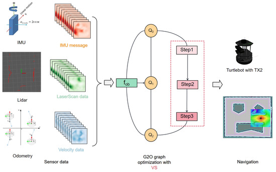
Figure 1.
Our architecture: (i) Real-time dynamic robot state information, , is acquired from sensors, encompassing variables such as position, orientation, and other pertinent data. (ii) In the method, the objective function is introduced as a new edge in the graph, replacing the original constraint. This step is pivotal for assimilating the results of the optimization process back into the overall trajectory planning framework. Steps 1–3 correspond to Formulas (5a)–(5c). (iii) General Graph Optimization (G2O) [32] is employed to solve the subproblem arising in the VS framework, where each vertex in the graph model denotes a state, and edges represent objective functions. (iv) The output of TEB-VS is the optimized trajectory for the robot.
2. Problem Formulation
We consider general TEB sequences of I robot configurations as
Here, represents the time interval, denotes the configuration of the robot pose, and is an initial parameter. , , and represent the x-directional position, the y-directional position, and the orientation of the robot in the map coordinate system, respectively. In each time interval, the robot transitions from the current configuration to the next configuration in the TEB sequence, . The primary objective is to derive the optimal TEB sequence, , as the trajectory.
Let be defined as the function associated with each robot configuration, . Given a set of robot configurations, , and corresponding time intervals, , our objective is to perform constrained optimization.
where represents the cost function, and serves as the weight for each function, . The parameters K and J denote the number of equality and inequality constraint functions, respectively, and and represent constraint functions—such as approximating the turning radius, enforcing maximum velocities, maximum accelerations, and minimum obstacle separation.
In TEB-VS, constraints encompass a series of equations or inequalities, incorporating dynamics constraints, collision avoidance constraints, and smoothness constraints. The objective function is employed to evaluate the trajectory’s quality, assessing the optimization’s effectiveness. Typically, factors such as smoothness, energy consumption, and time optimization are considered. Graph optimization involves converting the objective optimization problem into a hypergraph form and solving it using graph theory algorithms. Subsequently, either the Levenberg–Marquardt (LM) or Gauss–Newton (GN) method is employed for nonlinear optimization, initiating optimization iterations until convergence is reached. In the TEB-VS algorithm, VS is utilized instead of hard constraint methods, thereby facilitating smoother changes in the robot’s speed.
3. Methodology
In this section, we first introduce the framework of the proposed TEB-VS optimization method, and then we derive the augmented TEB algorithm to solve the subproblems arising within the steps of the method.
3.1. The General Framework
We exploit auxiliary variables to split the complex components, and we introduce a barrier function, , to replace the inequality-constrained function. We can rewrite (2) as an equality-constrained minimization problem.
Here, relaxes inequality constraints into equality forms, enabling closed-form updates. The penalty parameters balance constraint violations and trajectory smoothness.
To simplify the notation, we define the states , , and Lagrangian multipliers , . The augmented Lagrangian function is then defined as
where and are penalty parameters with the constraints, respectively. At each iteration, we can write
where n is the iteration number.
The symmetry principle manifests in two key aspects of our VS-based decomposition: first, in the balanced allocation of constraint weights between coupled variables (e.g., velocity vs. acceleration terms), ensuring the equivalent treatment of opposing optimization objectives; second, in the geometric symmetry of obstacle avoidance constraints, where radial distance penalties are isotropically enforced regardless of obstacle orientation. This dual symmetry enables coordinated updates through the augmented Lagrangian framework, preventing directional bias in trajectory adjustments.
In the objective function (2), acceleration and velocity optimization are among the applications of Lagrangian splitting. The velocity and acceleration can be minimax limits on velocity and acceleration. For the dual variable , we have the following subproblem:
and the solution in (5b) can be computed by
The primal function (5a) is non-convex and lacks a closed-form solution. Consequently, we employ the augmented TEB method to address this challenge in the following.
3.2. Augmented TEB for Solving -Subproblem
In this section, we propose the augmented TEB algorithm to solve the -subproblem arising in the VS framework. Typically, we have the objective function
The -subproblem combines smoothness costs , constraint penalties , and multiplier terms .
The problem of optimizing can be addressed by constructing the G2O hypergraph [12,32]. Utilizing a large-scale sparse matrix, the G2O serves as the optimization model. As depicted in Figure 1, the components of time and configuration are treated as nodes, while objective functions act as edges. The combination of nodes and edges forms the hypergraph. In the augmented TEB method, the classical constraint edges are transformed into objective functions using VS. This process involves representing the edges from traditional constraints to objective functions with VS techniques. The optimized edges and vertices resulting from this transformation are then incorporated into the sparse optimizer. Subsequently, the sparse optimizer generates the corresponding results. The hypergraph structure inherently preserves symmetry between temporal and spatial variables (e.g., time intervals, , and positional states, ). This symmetry-aware formulation ensures that updates to temporal and spatial parameters are equally weighted during optimization iterations, avoiding disproportionate emphasis on either trajectory smoothness or dynamic feasibility.
On the premise that the other input parameters of the TEB are unchanged, the speed constraint is replaced with (5) as an edge. In a similar manner, the VS method can be applied to handle other constraints and objectives within the trajectory-planning problem. For instance, if there are constraints related to waypoints, obstacles, and the fastest path, these can be reformulated and replaced using the VS method.
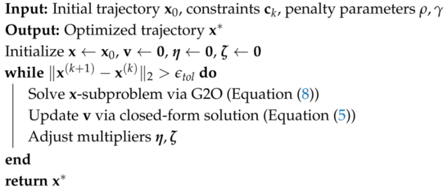
The workflow of TEB-VS is illustrated in Figure 2. First, real-time sensor data (e.g., position and obstacle distances) are fed into the VS module to decompose global constraints into subproblems. Next, the augmented TEB algorithm iteratively optimizes these subproblems using G2O, while symmetry principles ensure the balanced control of velocity and acceleration. Finally, the optimized trajectory is dynamically adjusted based on updated sensor feedback. This entire workflow is formalized and implemented through the TEB-VS algorithm, as detailed in Algorithm 1.
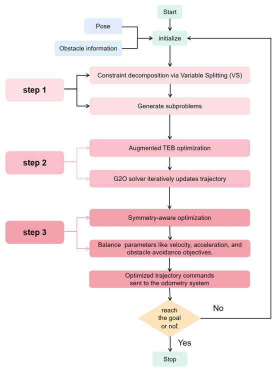
Figure 2.
Workflow of the TEB-VS Framework.
By decomposing global constraints into subproblems via variable splitting, the augmented TEB optimization leverages the inherent sparsity of the G2O hypergraph. This sparsity reduces the computational complexity of each inner iteration, offsetting the overhead introduced via outer-loop ADMM updates. Consequently, the overall complexity of TEB-VS remains comparable to classical TEB, as validated in Section 4.4.
| Algorithm 1: TEB-VS Algorithm. |
 |
4. Experiment and Analysis
In this section, we present an evaluation of the proposed algorithm using both simulated data and real-world trajectory planning applications. Firstly, we provide an overview of the algorithm’s performance in simulated environments. Secondly, we demonstrate its application in real robots. The results are presented and analyzed in both contexts.
Whether in simulation or on a real robot like the Turtlebot2, the navigation process with TEB-VS remains similar. As depicted in Figure 3, the Turtlebot2 chassis integrates odometry and an inertial measurement unit (IMU). Additionally, LIDAR sensors are incorporated to detect obstacle distances. The IMU interacts with the environment to constantly update the robot’s configuration, while odometry calculates and publishes the robot’s movements.
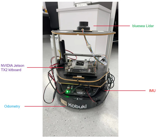
Figure 3.
Turtlebot2 is equipped with various sensors for perception and navigation, and the NVIDIA Jetson TX2 serves as the onboard computing platform. The combination of these components enables the robot to perceive its environment, plan trajectories, and execute navigation tasks autonomously.
Whether in simulation or on a real robot like the TurtleBot2, the navigation process with TEB-VS remains consistent. As depicted in Figure 3, the TurtleBot2 platform integrates odometry, an inertial measurement unit (IMU), and LIDAR sensors, which collectively enable real-time obstacle detection and configuration updates. This platform was selected for its academic relevance—its open-source modularity and ROS compatibility align with reproducibility standards in robotics research. Additionally, the integrated sensor suite (LIDAR for obstacle distances, IMU for orientation, and odometry for motion tracking) mimics real-world perception challenges, making it ideal for validating dynamic adaptability. To ensure rigorous benchmarking, we compare TEB-VS against classical TEB and DWA (industry-standard local planners for differential-drive robots) and the RANSAC method, a state-of-the-art variant focusing on obstacle simplification. These baselines collectively evaluate TEB-VS’s ability to harmonize trajectory smoothness with constraint handling in dynamic environments.
All pertinent parameters and equations, including constraints and objectives, are fed into the G2O framework for graph optimization. The optimization process aims to find the optimal velocity profile for the robot’s trajectory, considering various constraints and objectives. Once optimization is complete, the optimized velocity profile is sent to the odometry system, which translates it into physical movement commands for the robot.
4.1. Experimental Settings
All simulations were conducted in Gazebo/ROS with a TurtleBot2 model. The virtual machine configuration (Ubuntu 16.04, eight-core CPU, and 13.9 GB of RAM), and algorithm parameters (max speed = 0.3 m/s, sampling frequency = 10 Hz) are consistent across experiments unless stated otherwise.
The process begins with the establishment of the model world using Gazebo7, facilitated by the Gmapping function [38]. Subsequently, the SLAM method is employed to map this model world, resulting in the representation shown in Figure 4. In the OctoMap, each cell represents an area of one meter by one meter. The origin coordinate, located at the top left corner of the map, is defined as (0, 0). Once the Octomap is created [39], three distinct methods—DWA, TEB, and TEB-VS—are individually applied for autonomous trajectory planning. Each method is evaluated based on its performance in generating optimal trajectories within the simulated environment.
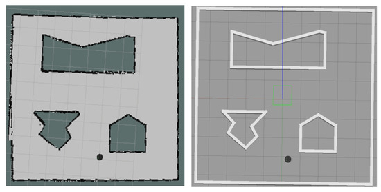
Figure 4.
Gazebo world navigation, the right part of this figure, shows the simulation room for Gazebo, and the left part is OctoMap [39] based on this room. The black point is the robot Turtlebot2. The details will also be updated on the map in real-world time during robot navigation in this room.
All simulations evaluate three key metrics:
- Path selection and trajectory: The chosen path and resulting trajectory within the simulated environment are monitored. This includes analyzing the smoothness, efficiency, and feasibility of the generated trajectories.
- Collision detection: The simulation environment is monitored for collisions. This ensures the safety and integrity of the robot’s movements throughout the simulation.
- Goal achievement: the simulation tracks whether the robot successfully reaches its intended goal or not.
4.1.1. Simulate Without Obstacle
In the evaluation process, both the TEB and DWA algorithms serve as baseline methods, providing trajectories that act as benchmarks. These trajectories are recorded for subsequent comparison against the results generated via the proposed algorithm. By conducting tests under identical experimental conditions, the velocity and trajectory outcomes of the proposed approach are systematically compared with those of the baseline algorithms. This comparative analysis facilitates an assessment of the performance and effectiveness of the proposed method. The experiment base in Figure 4 is used to simulate and test the accuracy and reach of the robot’s path planning under the premise of no dynamic obstacles, as well as the effect of TEB-VS method compared with the baseline method in robot motion control.
Considering that the robot operates on a two-dimensional plane, its motion is divided into two main stages: rotation, which is the path adjustment process, and linear motion, that is, the path tracking process, or it can be interpreted as the robot motion control process. This focused scrutiny ensures a robust and stable autonomous trajectory-planning process. The trajectories generated via all three algorithms originate from the same starting point and conclude at the same endpoint, facilitating direct comparison.
TEB, DWA, and TEB-VS algorithms all contain the same parameters, such as the velocity constraint, acceleration constraint, and obstacle distance constraint, and the same parameters were used in the experiments without special declarations. The algorithm terminated when the relative change in the augmented Lagrangian occurred after 50 iterations, balancing precision and efficiency. This setting enables the robot to operate within a relatively stable speed range and attempt to reach the maximum speed during linear motion. Other parameters, such as acceleration constraints and obstacle distance constraints, often employ default optimal values. Furthermore, the sampling frequency and final arrival tolerance are set to 10 Hz and 0.15 m, respectively, to ensure accuracy and real-time performance in all three algorithms.
4.1.2. Simulate with Obstacle
To evaluate dynamic obstacle handling, we extended the simulation to a warehouse environment with three human-shaped obstacles moving along predefined paths (Figure 5). The parameters remained identical to those in Section 4.1.1, and this test was based on three different algorithms: TEB, RANSAC, and TEB-VS.
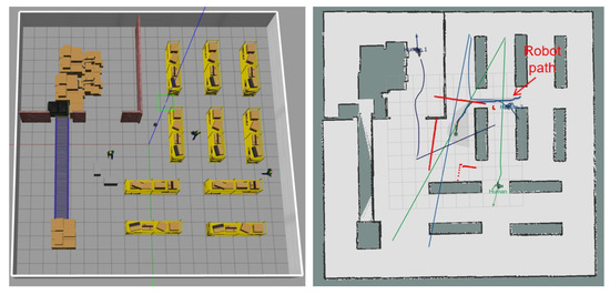
Figure 5.
The left picture shows the model of the warehouse, the robot, and the obstacle in a gazebo, and the right picture shows the Octomap of the warehouse. Corresponding OctoMap navigation analysis with coordinate grid (1 m resolution), where green purple and cyan solid lines denote preplanned trajectories of Human Obstacle 1, 2 and 3 respectively, the blue path with red directional arrows represents the robot’s optimized trajectory generated by TEB-VS, and red graphical elements (dotted lines: transient LiDAR detections; solid lines: confirmed obstacle boundaries) illustrate real-time perception updates.
4.2. Simulation Results
4.2.1. Results Without Obstacle
The autonomous trajectory-planning results generated via different methods are demonstrated in Figure 6. The method TEB-VS showcased in the figure outperforms the other algorithms in terms of trajectory-planning accuracy, resulting in a markedly superior trajectory. Additionally, the motion of the robot following this method exhibits smoother operation throughout the autonomous trajectory-planning process. It is important to note that all three algorithms successfully avoid obstacles and reach the destination.
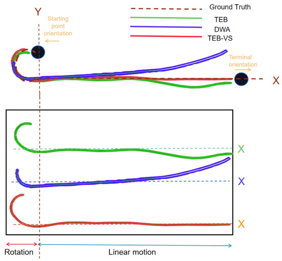
Figure 6.
Autonomous trajectory planning generated via different methods. The starting point is at coordinates (2, 5) with a specific orientation, and the goal is to navigate coordinates (9, 5) with a different orientation in the OctoMap. There are two phases of autonomous trajectory-planning motion: rotation and linear motion. The dotted lines are the ground truth. When comparing velocity stability, especially in the context of navigating the robot, it is important to distinguish between the rotational and linear processes. Special attention should be given to the left and right swings of the robot during the linear motion phase, as this significantly impacts the accuracy of reaching the endpoint. The symmetric distribution of velocity profiles further validates the balanced optimization achieved using TEB-VS.
On account of the motion path and maximum speed settings in the experiment being the same, the actual time in the simulation process is also similar. We conducted sampling, divided the whole motion process into M configurations, and obtained the velocity and angular velocity at each sampling point and recorded them. The rotational process spans from the first sampling point to the Dth sampling point, while the linear motion process extends from the th sampling point to the Mth sampling point. We consider the motion to be in a state of rotation when the angular velocity is sufficiently small and the linear velocity is close to its maximum and stable. Conversely, if the angular velocity is not negligible, the motion is considered to be in a state of rotation.
The comparison provided in Figure 7 offers insights into the changes in linear motion velocity, , during the rotation process. It is evident from the figure that all three algorithmic robots start from a near-stop state and gradually accelerate to their maximum velocities during rotation. In the case of DWA, the velocity, , undergoes a sudden change, starting slow and then rotating and moving forward at a very high speed. Conversely, TEB and TEB-VS divide the path into two sections, involving a small acceleration process to reach a certain speed before stabilizing, followed by reaching the maximum speed. This approach enhances the stability of robot control. Moreover, due to the increased internal iteration in TEB-VS, the robot exhibits smoother acceleration.
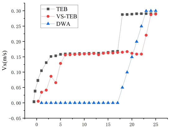
Figure 7.
Linear velocity variation of rotation. This graph illustrates the distribution of linear velocity for the first D sampling points of the three algorithms, specifically focusing on the linear velocity during rotation.
Figure 8 illustrates the distribution of angular velocity changes during the linear motion of the robot. As depicted, at the onset of linear motion, the robot from all three algorithm experiments returns to the vicinity of axis 0 from a high angular velocity, initiating oscillations, which represent the robot’s instability during motion. Closer proximity of the oscillation to 0 signifies better stability. The graph indicates that the distribution of VS-TEB is notably superior to that of DWA and TEB. Particularly, during the deceleration process near the endpoint, VS-TEB exhibits a smaller swing, enabling more accurate navigation to the endpoint.
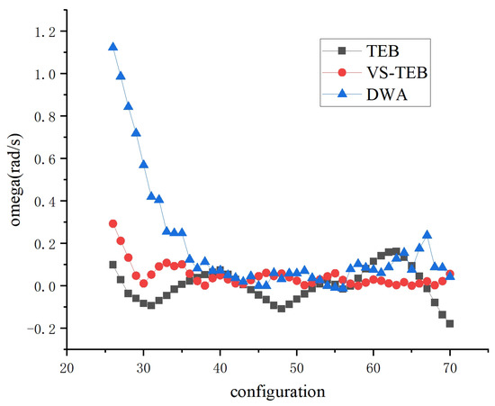
Figure 8.
Angular velocity variation of linear motion. This diagram illustrates the angular velocity distribution of linear motion from the st sampling point to the Mth sampling point, representing the oscillation of linear motion.
The testing methodology involves recording the speed difference between two consecutive sampling points, treating them as continuous states. A smaller speed difference between these states indicates enhanced stability in the trajectory during linear motion. Table 1 and Table 2 present the velocity variation results obtained during the simulation with different algorithms and velocities.

Table 1.
Velocity variation values generated via different methods in simulation (without obstacles).
Table 2.
Velocity variation values generated via different max velocities of TEB-VS in simulation (without obstacle).
Given that the sampling frequency aligns with the frequency of speed instruction issuance, we assume the speed of the Nth sampling point as . Before publishing the speed of the node , we consider the speed during this period to be . Thus, the speed can be regarded as a piecewise continuous distribution. Consequently, the key determinant of whether the robot can run stably lies in the difference between its angular velocity, and . When this difference is sufficiently small and exhibits regular distribution, we infer that the robot can navigate stably in straight-line motion. We conducted the following processing and calculations for the three sets of data:
- Mean Value
The mean value [40] refers to the mathematical expectation, which is calculated as the average of all angular velocity differences. A smaller average indicates less wobbling in the linear motion. We then write
The robot exhibited the best stability at 0.3 m/s, while the mean value of stability decreased at 0.5 m/s. Our analysis suggests that, as the linear speed of the robot increases, the time and amplitude of its angle adjustment will also change, resulting in a decline in its linear stability. However, when comparing TEB-VS with TEB and DWA, it is evident that its performance remains relatively stable. Moreover, it outperforms TEB and DWA when the maximum speed parameter is set to 0.3 m/s.
The comprehensive comparison of velocity stability shows that the TEB-VS method outperforms both the TEB and DWA methods. During the linear motion, the comparative analysis between the TEB-VS and TEB methods reveals that the angular velocity variation in the rotation phase is notably greater for the proposed method. TEB-VS exhibits significantly better angular velocity variation compared to both TEB and DWA, achieving optimizations of over and , respectively.
As shown in Table 3, TEB-VS exhibits a planning time of 0.0017 s, slightly higher than TEB’s 0.0005 s. However, both values are negligible compared to the 0.05 s cycle time of 20 Hz sampling (i.e., ≤3.4% of the cycle time), ensuring seamless integration into real-time control systems.
Table 3.
Algorithm run time test of simulation.
The traditional TEB algorithm encounters problems such as a control-quantity jump and an unstable running state in the actual control process of robot operation. RANSAC adopts the method of an optimal preview strategy to improve the control quantity of traditional TEB optimization output, while TEB-VS reduces the mutability of its control quantity through iteration so as to make the robot’s motion more stable and reliable.
Table 4 lists the variation values of the output control quantity of the three algorithms in an environment with dynamic obstacles. Compared with the traditional TEB algorithm and the improved RANSAC algorithm, the stability of TEB-VS algorithm can be improved by 37% and 15%, respectively.
Table 4.
Velocity variation values generated via different methods in simulation (with obstacle).
4.2.2. Results with Obstacle
4.3. Real-Life Robot Results
Like in the simulation, we deployed the algorithm with the robot to observe whether the robot runs more stably in the actual environment. Our robot platform, as shown in Figure 3, consists of an NVIDIA Jetson TX2 kitboard (Yujin Robot Co., Ltd., Seoul, South Korea), a Turtlebot2 chassis, and a bluesea lidar(LDS-50C-2, Lanhai Co., Ltd., Shanghai, China), all of which offer superior performance to support the algorithm. The NVIDIA Jetson TX2 kitboard provides substantial computational power, capable of achieving up to 1.33 TFLOPS (trillion floating-point operations per second). When coupled with the Ubuntu 16.04 operating system and ROS Kinetic Kame versions, it forms a robust platform for running the three algorithms under test reliably. The radar sensor integrated into the system accurately detects obstacle distances and reflection coefficients. Through processing with the Point Cloud Library (PCL), it effectively identifies obstacles and contributes to SLAM mapping functionality. The IMU serves to detect and measure acceleration and rotational motion, enabling the robot to understand its orientation and movement in space. By performing calculations based on IMU data, the relative position and motion of the robot can be determined and recorded. Odometry data, on the other hand, record the direction and distance traveled by the robot, providing essential information for navigation. During navigation tasks, odometry data serve as the primary basis for judgment, while IMU data help correct any discrepancies in direction and distance, ensuring the accuracy and reliability of the robot’s position and motion information.
Choosing the office shown in the top of Figure 9 as our experimental site offers several advantages for evaluating our algorithms:
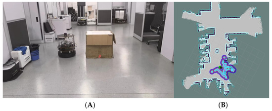
Figure 9.
(A) The left image displays the TurtleBot2 robot autonomously navigating through an office space while executing real-time obstacle avoidance, utilizing onboard computational resources for trajectory optimization. (B) The right image depicts the OctoMap generated through Gmapping SLAM (0.05 m resolution), where grey grid cells represent persistent structural features, cyan polygonal boundaries indicate real-time obstacle detections with 0.15 m inflation radius, and cyan rectangular markers in the middle of the office map denote a verified box-shaped obstacle. The robot’s estimated pose, shown as a black circular marker in the lower-right quadrant updates through sensor fusion of wheel odometry and IMU data.
- The uniform size of the office stations ensures that the environment contains many similar scenes. This characteristic poses higher demands on our SLAM mapping and navigation capabilities. While the radar’s role in assisting positioning may be limited, odometry and IMU data become crucial for determining the robot’s posture.
- By strategically placing obstacles within the office environment, we can increase the complexity of path planning and navigation tasks. This allows us to assess the algorithms’ performance in dynamic and challenging scenarios.
- The presence of people moving around the office adds an element of dynamic obstacle testing. This dynamic environment provides valuable insights into the algorithms’ ability to adapt and respond to changing conditions. Overall, the office environment serves as a realistic and challenging testbed for evaluating the effectiveness and robustness of our navigation algorithms.
Using the Gmapping algorithm, we generated an OctoMap through SLAM, resulting in a relatively reliable map of the environment. To assess the performance of our algorithms, we conducted a comparative test between the TEB algorithm and the TEB-VS algorithm on the Turtlebot2 robot. The bottom image of Figure 9 illustrates this testing scenario. Due to its limited obstacle avoidance capabilities, the performance of the DWA algorithm during actual operation falls significantly behind that of TEB-VS and TEB.
Similar to the simulation, we conducted tests on the actual speed change of the robot using the Turtlebot2 platform, and the results are presented in Table 5. The maximum speed parameters of the robot were also set to 0.3 m/s. The only difference from the simulation conclusion is that the stability optimization result reduced during linear motion, changing from 46.5% to 26.7%. However, this result still demonstrates a significant improvement over TEB.
Table 5.
Velocity variation values generated via different methods in real-life robot.
We also conducted comparative tests on the running time and velocity variation of the robots. Table 6 displays the running time of the TEB algorithm and the TEB-VS algorithm. The conclusion is similar to the result of the simulation: the running time of the TEB-VS algorithm can be neglected, introducing an iteratively smaller influence on the performance of the algorithm.
Table 6.
Algorithm running time test of real-life robot.
4.4. Parameter Sensitivity Analysis
The performance of ADMM-based TEB-VS depends on two key hyperparameters: the penalty parameter and the number of iterations.
A smaller (e.g., 0.001) allows constraints to be gradually satisfied, avoiding early over-penalization that may trap the optimization in local minima. Conversely, a larger (e.g., 1.0) enforces constraints aggressively but risks destabilizing the primal–dual balance.
In non-convex problems, sufficient iterations are required to ensure convergence to a local minimum. Tests showed that 20 iterations failed to stabilize residuals (velocity constraints unsatisfied), while 50 iterations achieved stable residuals with diminishing objective improvements as Figure 10 shows. This aligns with prior work [26], where 50 iterations empirically balanced convergence and computational cost.
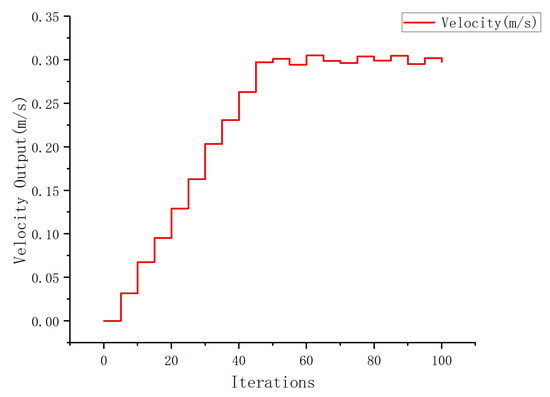
Figure 10.
The output of the robot’s control speed under different iterations.
To rigorously evaluate the computational scalability of TEB-VS, we conducted additional experiments with varying ADMM iteration counts (10, 50, and 100). As shown in Table 7, the planning time increases marginally from 0.0016 s to 0.0019 s as iterations grow, yet it remains well below the 0.05 s threshold for 20 Hz real-time control (i.e., ≤ of the cycle time). This demonstrates that TEB-VS maintains stable performance even under increased computational loads, validating its suitability for resource-constrained platforms.
Table 7.
TEB-VS running time under different iteration counts.
5. Conclusions
In this paper, we have proposed the TEB-VS algorithm, a novel trajectory planning framework that synergizes variable splitting strategies with timed-elastic-band optimization. The core innovations of this work address three interconnected challenges in autonomous navigation: First, by integrating symmetry-aware optimization principles into constraint decomposition, our method achieves a balanced trade-off between trajectory smoothness and dynamic constraints, delivering up to improvement in motion stability over classical TEB algorithms. Second, the computational efficiency of our approach enables the real-time resolution of non-convex planning problems, maintaining execution speeds comparable to TEB while effectively mitigating control oscillations during linear motion. Third, extensive validation across diverse environments—from obstacle-free simulations to dynamic scenarios ( stability gain with obstacles) and real-world office deployments ( angular control improvement)—demonstrates robust generalizability. These advancements offer tangible benefits to the research community: the framework provides a stable algorithmic foundation for resource-constrained autonomous platforms, introduces novel insights into symmetry-driven multi-objective optimization strategies, and facilitates reliable navigation in complex environments through our publicly available implementation.
Our evaluation framework focused on motion stability, angular control precision, and computational efficiency—metrics critical for real-world autonomous navigation. While ROC analysis is commonly applied to classification tasks (e.g., obstacle detection), trajectory planning requires continuous optimization metrics such as velocity variance, collision-free path rates, and goal achievement, all of which have been rigorously quantified in this work. Future studies will explore complementary evaluation dimensions, including trajectory deviation RMSE and energy consumption analysis, to address broader operational scenarios.
Despite these advancements, TEB-VS currently assumes ideal sensor inputs. Future work will extend the framework to handle sensor noise and partial observability. Additionally, we plan to integrate TEB-VS with high-level task planners for multi-robot systems.
Author Contributions
Conceptualization, H.Z. and R.G.; methodology, H.Z. and R.G.; software, K.J. and J.W.; validation, K.J.; formal analysis, R.G.; investigation, K.J.; writing—original draft preparation, H.Z. and R.G.; writing—review and editing, J.W. and R.S.; supervision, R.G. and R.S. All authors have read and agreed to the published version of the manuscript.
Funding
This work was supported by the Science and Technology Commission of Shanghai Municipality under Grant 2021SHZDZX, and the National Key Research and Development Program of China (2021ZD0202200, 2021ZD0202202), the National Natural Science Foundation of China (No. 52301402) and the Guangdong Basic and Applied Basic Research Foundation (No. 2022A1515110574). Rui Gao is affiliated with the Key Laboratory of Marine Intelligent Equipment and System of Ministry of Education, Shanghai Jiao Tong University, and Shenzhen Research Institute of Shanghai Jiao Tong University.
Data Availability Statement
The original contributions presented in the study are included in the article, further inquiries can be directed to the corresponding authors.
Conflicts of Interest
The authors declare no conflicts of interest.
References
- Li, M.; Cheng, N.; Gao, J.; Wang, Y.; Zhao, L.; Shen, X. Energy-efficient UAV-assisted mobile edge computing: Resource allocation and trajectory optimization. IEEE Trans. Veh. Technol. 2020, 69, 3424–3438. [Google Scholar] [CrossRef]
- Li, X.; Ahn, C.K.; Zhang, W.; Shi, P. Asynchronous Event-Triggered-Based Control for Stochastic Networked Markovian Jump Systems With FDI Attacks. IEEE Trans. Syst. Man Cybern. 2023, 53, 5955–5967. [Google Scholar] [CrossRef]
- Ma, J.; Cheng, Z.; Zhang, X.; Tomizuka, M.; Lee, T.H. Alternating Direction Method of Multipliers for Constrained Iterative LQR in Autonomous Driving. IEEE Trans. Intell. Transp. Syst. 2020, 23, 23031–23042. [Google Scholar] [CrossRef]
- Gao, R.; Särkkä, S.; Claveria-Vega, R.; Godsill, S. Autonomous tracking and state estimation with generalised group Lasso. IEEE Trans. Cybern. 2021, 52, 12056–12070. [Google Scholar] [CrossRef]
- Tan, Y.; Deng, H.; Sun, M.; Zhou, M.; Chen, Y.; Chen, L.; Wang, C.; An, F. A Reconfigurable Coprocessor for Simultaneous Localization and Mapping Algorithms in FPGA. IEEE Trans. Circuits Syst. II Express Briefs 2022, 70, 286–290. [Google Scholar] [CrossRef]
- Liu, Y.; Huang, K.; Zhao, N.; Li, J.; Hao, S.; Huang, Z.; Qi, X.; Wang, X.; Zhou, L.; Chang, L.; et al. BOHA: A High Performance VSLAM Backend Optimization Hardware Accelerator using Recursive Fine-Grain H-Matrix Decomposition and Early-Computing with Approximate Linear Solver. IEEE Trans. Circuits Syst. II Express Briefs 2023, 70, 3827–3831. [Google Scholar] [CrossRef]
- Lu, X.; Jia, Y. Trajectory Planning of Free-Floating Space Manipulators With Spacecraft Attitude Stabilization and Manipulability Optimization. IEEE Trans. Syst. Man Cybern. 2021, 51, 7346–7362. [Google Scholar] [CrossRef]
- Dijkstra, E.W. A Note on Two Problems in Connection with Graphs. In Edsger Wybe Dijkstra: His Life, Work, and Legacy; Association for Computing Machinery: New York, NY, USA, 2022; pp. 287–290. [Google Scholar]
- Duchoň, F.; Babinec, A.; Kajan, M.; Beňo, P.; Florek, M.; Fico, T.; Jurišica, L. Path planning with modified a star algorithm for a mobile robot. Procedia Eng. 2014, 96, 59–69. [Google Scholar] [CrossRef]
- Hart, P.E.; Nilsson, N.J.; Raphael, B. A formal basis for the heuristic determination of minimum cost paths. IEEE Trans. Syst. Man Cybern. Syst. 1968, 4, 100–107. [Google Scholar] [CrossRef]
- Fox, D.; Burgard, W.; Thrun, S. The dynamic window approach to collision avoidance. IEEE Robot. Autom. Mag. 1997, 4, 23–33. [Google Scholar] [CrossRef]
- Rösmann, C.; Feiten, W.; Wösch, T.; Hoffmann, F.; Bertram, T. Trajectory modification considering dynamic constraints of autonomous robots. In Proceedings of the 7th German Conference on Robotics, Munich, Germany, 21–22 May 2012; pp. 1–6. [Google Scholar]
- Zhang, H.; Dou, L.; Fang, H.; Chen, J. Autonomous indoor exploration of mobile robots based on door-guidance and improved dynamic window approach. In Proceedings of the IEEE International Conference on Robotics and Biomimetics, Guilin, China, 19–23 December 2009; pp. 408–413. [Google Scholar]
- Smith, J.S.; Xu, R.; Vela, P. EGOTEB: Egocentric, perception space navigation using timed-elastic-bands. In Proceedings of the IEEE International Conference on Robotics and Automation, Paris, France, 31 May–31 August 2020; pp. 2703–2709. [Google Scholar]
- Sun, Y.; Chu, Y.; Xu, T.; Li, J.; Ji, X. Inverse Reinforcement Learning Based: Segmented Lane-Change Trajectory Planning with Consideration of Interactive Driving Intention. IEEE Trans. Veh. Technol. 2022, 71, 11395–11407. [Google Scholar] [CrossRef]
- Li, H.; Chen, P.; Yu, G.; Zhou, B.; Li, Y.; Liao, Y. Trajectory Planning for Autonomous Driving in Unstructured Scenarios Based on Deep Learning and Quadratic Optimization. IEEE Trans. Veh. Technol. 2023, 73, 4886–4903. [Google Scholar] [CrossRef]
- Glowinski, R.; Osher, S.J.; Yin, W. Splitting Methods in Communication, Imaging, Science, and Engineering; Springer: Cham, Switzerland, 2017. [Google Scholar]
- Wright, S.J.; Nocedal, J. Numerical Optimization; Springer: Berlin/Heidelberg, Germany, 2006. [Google Scholar]
- Eckstein, J.; Bertsekas, D. On the Douglas-Rachford Splitting Method and the Proximal Point Algorithm for Maximal Monotone Operators. Math. Program. 1992, 55, 293–318. [Google Scholar] [CrossRef]
- Ryu, E.; Boyd, S.P. A primer on monotone operator methods. Appl. Comput. Math. 2016, 15, 3–43. [Google Scholar]
- Peaceman, D.W.; Rachford, H.H. The numerical solution of parabolic and elliptic differential equations. J. Soc. Indust. Appl. Math. 1955, 3, 28–41. [Google Scholar] [CrossRef]
- He, B.S.; Liu, H.; Wang, Z.R.; Yuan, X.M. A strictly contractive Peaceman–Rachford splitting method for convex programming. SIAM J. Optim. 2014, 24, 1011–1040. [Google Scholar] [CrossRef]
- Chambolle, A.; Pock, T. A first-order primal-dual algorithm for convex problems with applications to imaging. J. Math. Imaging. Vis. 2011, 40, 120–145. [Google Scholar] [CrossRef]
- Goldstein, T.; Osher, S. The Split Bregman Method for L1-Regularized Problems. SIAM J. Imaging Sci. 2009, 2, 323–343. [Google Scholar] [CrossRef]
- Boyd, S.; Parikh, N.; Chu, E.; Peleato, B.; Eckstein, J. Distributed optimization and statistical learning via the alternating direction method of multipliers. Found. Trends Mach. Learn. 2011, 3, 1–122. [Google Scholar] [CrossRef]
- Gao, R.; Tronarp, F.; Sarkka, S. Variable splitting methods forconstrained state estimation in partially observed Markov processes. IEEE Signal Process. Lett. 2020, 27, 1305–1309. [Google Scholar] [CrossRef]
- Katoch, S.; Chauhan, S.S.; Kumar, V. A review on genetic algorithm: Past, present, and future. Multimed. Tools Appl. 2021, 80, 8091–8126. [Google Scholar] [CrossRef] [PubMed]
- Amine, K. Multiobjective simulated annealing: Principles and algorithm variants. Adv. Oper. Res. 2019, 2019, 8134674. [Google Scholar] [CrossRef]
- Oliva, D.; Esquivel-Torres, S.; Hinojosa, S.; Pérez-Cisneros, M.; Osuna-Enciso, V.; Ortega-Sánchez, N.; Dhiman, G.; Heidari, A.A. Opposition-based moth swarm algorithm. Expert Syst. Appl. 2021, 184, 115481. [Google Scholar] [CrossRef]
- Zhu, H.; Zhou, M.; Alkins, R. Group role assignment via a Kuhn–Munkres algorithm-based solution. IEEE Trans. Syst. Man. Cybern. A Syst. Hum. 2011, 42, 739–750. [Google Scholar] [CrossRef]
- Xu, Z.; Li, Z.; Guan, Q.; Zhang, D.; Li, Q.; Nan, J.; Liu, C.; Bian, W.; Ye, J. Large-scale order dispatch in on-demand ride-hailing platforms: A learning and planning approach. In Proceedings of the 24th ACM SIGKDD International Conference on Knowledge Discovery & Data Mining, London, UK, 19–23 August 2018; pp. 905–913. [Google Scholar]
- Kummerle, R.; Grisetti, G.; Strasdat, H.; Konolige, K.; Burgard, W. G2O: A general framework for graph optimization. In Proceedings of the IEEE International Conference on Robotics Automation, Shanghai, China, 9–13 May 2011; pp. 3607–3613. [Google Scholar]
- Wang, Y. Gauss–newton method. Wiley Interdiscip. Rev. Comput. Stat. 2012, 4, 415–420. [Google Scholar] [CrossRef]
- Moré, J.J. The Levenberg-Marquardt algorithm: Implementation and theory. In Numerical Analysis: Proceedings of the Biennial Conference, Dundee, UK, 28 June–1 July 1977; Springer: Berlin/Heidelberg, Germany, 2006; pp. 105–116. [Google Scholar]
- Liu, C.; Liu, Y. Robot planning and control method based on improved time elastic band algorithm. In Proceedings of the 2023 4th International Conference on Computer Engineering and Application (ICCEA), Hangzhou, China, 7–9 April 2023; pp. 911–915. [Google Scholar]
- Zhao, J.; Zhang, J.; Liu, H.; Wang, J.; Chen, Z. Path planning for a tracked robot traversing uneven terrains based on tip-over stability. Asian J. Control 2023, 25, 3569–3583. [Google Scholar] [CrossRef]
- Ramadasan, D.; Chevaldonné, M.; Chateau, T. LMA: A generic and efficient implementation of the Levenberg–Marquardt Algorithm. Softw. Pract. Exp. 2017, 47, 1707–1727. [Google Scholar] [CrossRef]
- Grisetti, G. Improving Gridbased SLAM with Rao-Blackwellized Particle Filters by Adaptive Proposals and Selective Resampling. In Proceedings of the 2005 IEEE International Conference on Robotics and Automation, Barcelona, Spain, 18–22 April 2005. [Google Scholar]
- Hornung, A.; Wurm, K.M.; Bennewitz, M.; Stachniss, C.; Burgard, W. OctoMap: An efficient probabilistic 3D mapping framework based on octrees. In Autonomous Robots; Springer: New York, NY, USA, 2013. [Google Scholar]
- Elliott, P.D.T.A. Probabilistic Number Theory I: Mean-Value Thoerems; Springer: New York, NY, USA, 1979. [Google Scholar]
Disclaimer/Publisher’s Note: The statements, opinions and data contained in all publications are solely those of the individual author(s) and contributor(s) and not of MDPI and/or the editor(s). MDPI and/or the editor(s) disclaim responsibility for any injury to people or property resulting from any ideas, methods, instructions or products referred to in the content. |
© 2025 by the authors. Licensee MDPI, Basel, Switzerland. This article is an open access article distributed under the terms and conditions of the Creative Commons Attribution (CC BY) license (https://creativecommons.org/licenses/by/4.0/).