The New Gompertz Distribution Model and Applications

Abstract

The Gompertz distribution has long been a cornerstone for analyzing growth processes and mortality patterns across various scientific disciplines. However, as the intricacies of real-world phenomena evolve, there is a pressing need for more versatile probability distributions that can accurately capture a wide array of data characteristics. In response to this demand, we introduce the Marshall–Olkin Power Gompertz (MOPG) distribution, an innovative and powerful extension of the traditional Gompertz model. The MOPG distribution is crafted by enhancing the Power Gompertz cumulative distribution function through the Marshall–Olkin transformation. This distribution yields two pivotal contributions: a power parameter (c) that significantly increases the model’s adaptability to diverse data patterns and the Marshall–Olkin transformation, which modifies tail behavior to enhance predictive accuracy. Furthermore, we derived the distribution’s essential statistical properties and evaluate its performance through extensive Monte Carlo simulations, along with a maximum likelihood estimation of model parameters. Our empirical validation, utilizing three real-world data sets, compellingly demonstrated that the MOPG distribution not only surpasses several well-established lifetime distributions but is also superior in terms of flexibility and tail behavior characterization. The results highlight that the proposed MOPG stands out as a superior choice, delivering the most precise fit to the data when compared to various competing models, and its performance makes it a compelling option worth considering.

1. Introduction

In recent years, the development of flexible statistical models has become increasingly important in fields such as reliability engineering, survival analysis, and biomedical statistics. Among these, the Gompertz distribution has long been favored for describing aging and mortality processes due to its ability to represent increasing hazard functions. These models introduce additional parameters to enhance flexibility, but they may still fall short in modeling the full range of data characteristics observed in practice. Specifically, their ability to capture extreme events and tail behavior remains constrained, particularly in data sets with heterogeneous or multimodal features. In response to these challenges, we propose a new four-parameter lifetime distribution: the Marshall–Olkin Power Gompertz (MOPG) distribution. This model is constructed by applying the Marshall–Olkin transformation to the cumulative distribution function of the Power Gompertz distribution. The resulting distribution is more flexible and can accommodate a wider array of hazard rate shapes, including increasing, decreasing, bathtub-shaped, and unimodal patterns. Two key elements contribute to the model’s adaptability: a power parameter that enhances shape control and the Marshall–Olkin mechanism that adjusts tail heaviness, offering a significant improvement in data fitting and interpretation. Recently, a number of methods have been proposed to fit various kinds of data and provide extremely accurate distributions. The Gompertz law of human mortality was originally introduced by Gompertz in 1824 [1]. The alpha Power Gompertz distribution was explored in detail by Eghwerido et al. [2]. Khan et al. [3] presented the transmuted Gompertz distribution and its estimation methods. An extension of this model, the transmuted generalized Gompertz distribution, was studied by Khan, King, and Hudson [4]. Benkhelifa [5] introduced the Marshall–Olkin extended generalized Gompertz distribution. Eghwerido et al. [6] proposed the inverse odd Weibull generated family of distributions. The shifted exponential-G family and its applications were studied by Eghwerido, Agu, and Ibidoja [7]. Eghwerido and Agu [8] examined the shifted Gompertz-G family in their work. The alpha power Teissier distribution was introduced by Eghwerido [9]. A new Kumaraswamy-alpha power inverted exponential distribution was developed by Thomas et al. [10]. Eghwerido, Oguntunde, and Agu [11] introduced the alpha power Marshall–Olkin–G distribution. The Gompertz extended generalized exponential distribution was discussed by Eghwerido et al. [12]. Eghwerido, Zelibe, and Efe-Eyefia [13] proposed the Gompertz-alpha power inverted exponential distribution. Alzaatreh et al. [14] introduced a general method for generating continuous distribution families. Mahdavi and Kundu extended the exponential distribution using a new generating method [15]. Marshall and Olkin [16] presented a classical method for adding a parameter to distribution families. Eghwerido, Ogbo, and Omotoye [17] proposed the Marshall–Olkin Gompertz distribution. This paper focuses on the Marshall–Olkin Power Gompertz (MOPG) distribution, a four-parameter model designed for lifetime processes. It establishes the statistical structural properties of this suggested distribution and develops a closed form for the maximum likelihood estimates (MLEs) of the MOPG parameters. The probability density function of the Gompertz distribution is provided as follows:

$$g\left(x\right)=aexp\left(bx+a/b\left(1-exp\left(bx\right)\right)\right),x,a,b>0.$$

(1)

The cumulative distribution function that corresponds to Equation (1) is defined as follows:

$$G\left(x\right)=1-exp\left(-{\displaystyle \frac{a}{b}}\left(exp\left(bx\right)-1\right)\right),x,a,b>0,$$

(2)

where a and b are parameters. Similarly, the probability density function of the Power Gompertz distribution is presented as

$$g\left(x\right)=ac{x}^{c-1}exp\left(b{x}^c-a/b\left(exp\left(b{x}^c\right)-1\right)\right),x,a,b,c>0.$$

(3)

The equivalent cumulative distribution function for Equation (3) is defined as

$$G\left(x\right)=1-exp\left(-a/b\left(exp\left(b{x}^c\right)-1\right)\right),x,a,b,c>0.$$

(4)

Assume that the baseline distribution or model has density and cumulative functions denoted by $g\left(x\right)$ and $G\left(x\right)$. A transformation to incorporate the Marshall–Olkin parameter with the given cumulative distribution function was proposed by [16] as follows

$$F\left(x\right)={\displaystyle \frac{G\left(x\right)}{d+(1-d)G\left(x\right)}},x,d>0.$$

(5)

Nonetheless, the associated PDF is stated as

$$f\left(x\right)={\displaystyle \frac{dg\left(x\right)}{{\left[d+(1-d)G\left(x\right)\right]}^2}},d>0.$$

(6)

This study is organized as follows: Section 1 introduces the Marshall–Olkin Power Gompertz (MOPG) distribution, an extension of the Power Gompertz distribution using the Marshall–Olkin transformation to improve flexibility and tail behavior modeling. Section 2 presents the MOPG distribution, including its probability density function (PDF), cumulative distribution function (CDF), survival function, and a 3D density plot. We also examine two key theoretical properties: identifiability (ensuring unique parameter identification) and asymptotic behavior (analyzing limits as the variable approaches zero and infinity). Section 3 explores the MOPG’s structural properties, such as the quantile function, moments (mean, variance, skewness, and kurtosis), Renyi entropy, and order statistics. Parameter estimation via maximum likelihood (MLE) is discussed, with computations performed using Newton–Raphson in R. Section 4 conducts simulation studies to assess MOPG’s performance under varying sample sizes and parameter settings. The results show that bias and the RMSE decrease as the sample size increases, confirming the MLE’s consistency. Section 5 applies the MOPG distribution to three real data sets: Italy COVID-19 case data, Bladder cancer remission times, and U.S. COVID-19 daily statistics. Model comparisons with Gompertz, Power Gompertz, Marshall–Olkin Gompertz, Gamma, and Weibull distributions are made using goodness-of-fit tests (KS, AD, AIC, and BIC). The MOPG consistently outperforms competitors, demonstrating superior flexibility in capturing complex data structures, especially in tail behavior. Section 6 summarizes key findings and concludes this study.

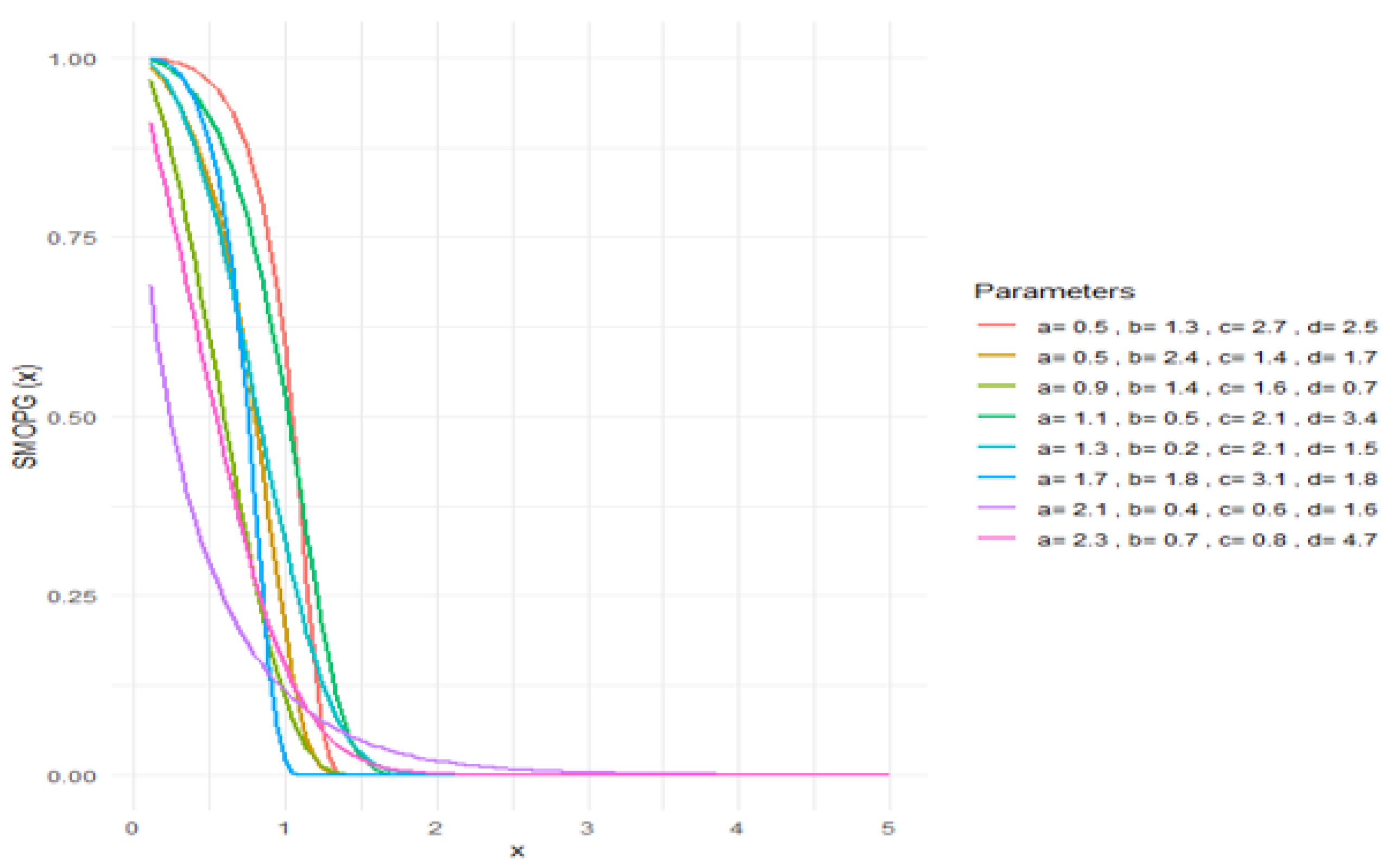
2. The Marshall–Olkin Power Gompertz (MOPG) Distribution

The newly suggested MOPG distribution with four parameters is presented in this section. If X is a continuous random variable, the pdf of the MOPG distribution can be expressed as

$$f_{MOPG}\left(x\right)={\displaystyle \frac{adc{x}^{c-1}exp\left(b{x}^c-a/b\left(exp\left(b{x}^c\right)-1\right)\right)}{{\left(d+\left(1-d\right)\left(1-exp\left(-a/b\left(exp\left(b{x}^c\right)-1\right)\right)\right)\right)}^2}},x,a,b,c,d>0.$$

(7)

A function $f_{MOPG}\left(x\right)$ qualifies as a probability density function if it fulfills the following two essential conditions: $f_{MOPG}\left(x\right)\ge 0$ for all x in its domain and ${\int }_0^{\infty }{f}_{MOPG}\left(x\right)dx=1$. For Equation (7), where $x>0$, $a,b,c,d>0$. Numerator: $a,d,c>0$, $x^{c-1}>0$ (since $x>0$ and $c>0$). The exponential function

$$exp\left(b{x}^c-{\displaystyle \frac{a}{b}}\left(exp\left(b{x}^c\right)-1\right)\right),$$

is always positive. Thus, the numerator is always positive. Denominator: since $d>0$ and

$$exp\left(-{\displaystyle \frac{a}{b}}\left(exp\left(b{x}^c\right)-1\right)\right)>0,$$

the term is

$$1-exp\left(-{\displaystyle \frac{a}{b}}\left(exp\left(b{x}^c\right)-1\right)\right)\in (0,1).$$

The denominator is a squared term, so it is always positive. $f_{MOPG}\left(x\right)\ge 0$ for all $x>0$. After, we must show that

$${\int }_0^{\infty }{f}_{MOPG}\left(x\right)dx=1.$$

Let

$$u={\displaystyle \frac{a}{b}}\left(exp\left(b{x}^c\right)-1\right).$$

Then, the derivative is

$${\displaystyle \frac{du}{dx}}=ac{x}^{c-1}exp\left(b{x}^c\right).$$

Rearranging

$$dx={\displaystyle \frac{du}{ac{x}^{c-1}exp\left(b{x}^c\right)}}.$$

The exponential term in the numerator becomes

$$exp\left(b{x}^c-u\right)=exp\left(b{x}^c\right)·e^{-u}.$$

Substituting $exp\left(b{x}^c\right)={\displaystyle \frac{bu}{a}}+1$, we obtain

$$exp(b{x}^c-u)=\left({\displaystyle \frac{bu}{a}}+1\right)e^{-u}.$$

Now, the PDF transforms as

$$f_{MOPG}\left(x\right)dx={\displaystyle \frac{adc{x}^{c-1}\left(\frac{bu}{a}+1\right)e^{-u}}{{\left[d+(1-d)(1-e^{-u})\right]}^2}}·{\displaystyle \frac{du}{ac{x}^{c-1}\left(\frac{bu}{a}+1\right)}}.$$

Simplifying:

$$f_{MOPG}\left(x\right)dx={\displaystyle \frac{d{e}^{-u}}{{\left[d+(1-d)(1-e^{-u})\right]}^2}}du.$$

Thus, the PDF becomes

$$f\left(u\right)du={\displaystyle \frac{d{e}^{-u}}{{\left[1-(1-d)e^{-u}\right]}^2}}du,$$

$u\in [0,\infty )$:

Let $v=e^{-u}$, then $dv=-e^{-u}du$, and the integral becomes

$${\int }_0^{\infty }{\displaystyle \frac{d{e}^{-u}}{{\left[1-(1-d)e^{-u}\right]}^2}}du=d{\int }_1^0{\displaystyle \frac{-dv}{{\left(1-(1-d)v\right)}^2}}=d{\int }_0^1{\displaystyle \frac{dv}{{\left(1-(1-d)v\right)}^2}}.$$

Now, let $w=1-(1-d)v$; then, $dw=-(1-d)dv$, and the integral becomes

$$d{\int }_1^d{\displaystyle \frac{-dw/(1-d)}{w^2}}={\displaystyle \frac{d}{1-d}}{\left[{\displaystyle \frac{1}{w}}\right]}_d^1={\displaystyle \frac{d}{1-d}}\left(1-{\displaystyle \frac{1}{d}}\right)={\displaystyle \frac{d}{1-d}}·{\displaystyle \frac{d-1}{d}}=1.$$

Since $f_{MOPG}\left(x\right)$ satisfies both conditions:

• $f_{MOPG}\left(x\right)\ge 0$,
• ${\int }_0^{\infty }{f}_{MOPG}\left(x\right)dx=1$,

it is a probability density function. The equivalent cumulative distribution function (cdf) is defined as follows:

$$F_{MOPG}\left(x\right)={\displaystyle \frac{1-exp\left(-a/b\left(exp\left(b{x}^c\right)-1\right)\right)}{d+(1-d)\left(1-exp\left(-a/b\left(exp(b{x}^c\right)-1\right)\right)}},a,b,c,d>0,$$

(8)

where d is a parameter. The plots for various parameter value scenarios are presented in Figure 1 and Figure 2. These graphs demonstrate that the MOPG density and cumulative distribution can exhibit unimodal characteristics, a rightward tilt, and a declining trend. Utilizing Equation (7) with parameters $d=1,c=1$, we derive the Gompertz distribution. As b approaches zero, we obtain the Weibull distribution. Additionally, with $c=1$, we arrive at the Marshall–Olkin Gompertz distribution [17]. The equations are as follows:

$$f_{MO-G}\left(x\right)={\displaystyle \frac{adexp\left(bx-a/b\left(exp\left(bx\right)-1\right)\right)}{{\left(1-\left(1-d\right)\left(exp\left(-a/b\left(exp\left(bx\right)-1\right)\right)\right)\right)}^2}},x,a,b,d>0,$$

(9)

$$F_{\mathrm{MO}\text{-}\mathrm{G}}\left(x\right)={\displaystyle \frac{1-exp\left(-\frac{a}{b}\left(exp\left(bx\right)-1\right)\right)}{1-(1-d)\left(exp\left(-\frac{a}{b}\left(exp\left(bx\right)-1\right)\right)\right)}},a,b,d>0.$$

(10)

The MOPG distribution’s survival function is described as follows:

$$S_{MOPG}\left(x\right)=1-\left({\displaystyle \frac{1-exp\left[-a/b\left(exp\left(b{x}^c\right)-1\right)\right]}{d+(1-d)\left[1-exp\left(-a/b\left(exp(b{x}^c\right)-1\right)\right]}}\right),a,b,c,d>0.$$

The MOPG distribution’s hazard rate function is written as follows:

$$h_{MOPG}\left(x\right)={\displaystyle \frac{\frac{adc{x}^{c-1}exp\left(b{x}^c-a/b\left(exp\left(b{x}^c\right)-1\right)\right)}{{\left(d+\left(1-d\right)\left(1-exp\left(-a/b\left(exp\left(b{x}^c\right)-1\right)\right)\right)\right)}^2}}{1-\left(\frac{1-exp\left(-a/b\left(exp\left(b{x}^c\right)-1\right)\right)}{d+(1-d)\left(1-exp\left(-a/b\left(exp(b{x}^c\right)-1\right)\right)}\right)}},a,b,c,d>0.$$

The MOPG survival function and hazard rate function plots for several parameter values are shown in Figure 3. The plots indicate that the MOPG dispersion is increasing and taking on a bathtub shape.

2.1. Mathematical Mixture Representation

The generated mixture representation would facilitate the explicit simplification of the suggested MOPG model’s characteristics. Furthermore, it would assist in expressing the Gompertz distribution of the proposed MOPG distribution. Nevertheless, for $\left|f\right|<1,\lambda >0$, then

$${\left(1-f\right)}^{-\lambda }=\sum _{\omega =0}^{\infty }\left(\begin{array}{c}\lambda +\omega -1\\ \omega \end{array}\right)f^{\omega },$$

(11)

for a real non-integer. Nevertheless, for the $\lambda$ integer, $\omega$ stops at $\omega -1$. Assuming that B is the quantity in Equation (7)’s denomination, $\Delta$ can be listed as

$$\Delta =\sum _{\omega =0}^{\infty }\left(\begin{array}{c}\lambda +\omega -1\\ \omega \end{array}\right){\left(1-d\right)}^{\omega }{\left(exp\left(-{\displaystyle \frac{a}{b}}\left(exp\left(b{x}^c\right)-1\right)\right)\right)}^{\omega }.$$

Consequently, the MOPG distribution can be described as a power series as

$$f_{MOPG}\left(x\right)=\sum _{\omega =0}^{\infty }\left(\begin{array}{c}\lambda +\omega -1\\ \omega \end{array}\right){\left(1-d\right)}^{\omega }da{x}^{c-1}exp\left(b{x}^c-{\displaystyle \frac{a}{b}}\left(exp\left(b{x}^c\right)-1\right)(\omega +1)\right).$$

(12)

2.2. Identifiability

Let ${\theta }_1=\left(a_1,b_1,c_1,d_1\right)$ and ${\theta }_2=\left(a_2,b_2,c_2,d_2\right)$ be two distinct parameter vector of the MOPG distribution. If the cumulative distribution functions satisfy $F\left(x;{\theta }_1\right)=F\left(x;{\theta }_2\right)$ for all $x>0,$ then ${\theta }_1={\theta }_2$. From Equation (8), assume $F\left(x;{\theta }_1\right)=F\left(x;{\theta }_2\right)$, $\forall x>0.$ Then, their logarithmic derivatives must also be ${\displaystyle \frac{dlog\left(F;{\theta }_1\right)}{dx}}={\displaystyle \frac{dlog\left(F;{\theta }_2\right)}{dx}}$. In Equation (8), we consider the transformation $G(x;\theta )=1-exp\left(-a/b\left(exp\left(b{x}^c\right)-1\right)\right)$, and this yields the functional equation $G\left(x;{\theta }_1\right)/\left(d_1+\left(1-d_1\right)G\left(x;{\theta }_1\right)\right)=G\left(x;{\theta }_2\right)/\left(d_2+\left(1-d_2\right)G\left(x;{\theta }_2\right)\right)$. In this equation, $x\to 0$, substituting into the functional equation reveals $a_1{x}^{c_1}=a_2{x}^{c_2}$, and for this to hold, $\forall x>0,$ we must have $c_1=c_2$ and $a_1=a_2$. As $x\to \infty$, $d_1=d_2$. Now with $a_1=a_2$, $c_1=c_2$ and $d_1=d_2$, we examine the remaining parameter b, and the term $exp\left(b{x}^c\right)$ must grow at the same rate for both distributions; thus, $b_1=b_2$.

2.3. Asymptotic Findings

We will develop certain asymptotic findings for the MOPG distribution. Referring to Section 1, we obtain the following equivalences as $x\to 0$, and we yield

$$\underset{x\to 0^{+}}{lim}f\left(x\right)=\left\{\begin{array}{ccc}f\left(x\right)\to \infty & ,& c<1\\ f\left(x\right)={\displaystyle \frac{ac}{d}}& ,& c=1\\ f\left(x\right)=0& & c>1\end{array}\right.$$

and for $hrf\left(x\right)$, $x\to 0$:

$$\underset{x\to 0^{+}}{lim}hrf\left(x\right)=\left\{\begin{array}{ccc}hrf\left(x\right)\to \infty & ,& c<1\\ hrf\left(x\right)={\displaystyle \frac{a}{d}}& ,& c=1\\ hrf\left(x\right)=0& & c>1.\end{array}\right.$$

3. Characteristics Structure of the MOPG Distribution

Several statistical structural features of the MOPG distribution are derived and examined in this section. These consist of the order statistics, quantile function, and the MLE.

3.1. Quantile Function of the MOPG Distribution

Let X be a random variable such that $X\sim \mathrm{MOPG}(a,b,c,d).$ The quantile function of X, denoted in terms of $u\in [0,1]$, is given in Equation (13) and illustrated in Figure 4,

$$Q_u\left(u\right)={\left({\displaystyle \frac{1}{b}}ln\left(1-{\displaystyle \frac{b}{a}}ln\left({\displaystyle \frac{1-u}{1-u(1-d)}}\right)\right)\right)}^{1/c},u\in [0,1].$$

(13)

Nevertheless, by using Equation (13), where u as 0.5 is chosen, we obtain the median (M) of X as

$$M={\left({\displaystyle \frac{1}{b}}ln\left(1-{\displaystyle \frac{b}{a}}ln\left({\displaystyle \frac{0.5}{1-0.5(1-d)}}\right)\right)\right)}^{1/c},u\in [0,1].$$

(14)

On the other hand, the random variable X’s 25th and 75th percentiles are determined as

$$Q_1={\left({\displaystyle \frac{1}{b}}ln\left(1-{\displaystyle \frac{b}{a}}ln\left({\displaystyle \frac{0.75}{1-0.25(1-d)}}\right)\right)\right)}^{1/c},$$

(15)

$$Q_3={\left({\displaystyle \frac{1}{b}}ln\left(1-{\displaystyle \frac{b}{a}}ln\left({\displaystyle \frac{0.25}{1-0.75(1-d)}}\right)\right)\right)}^{1/c}.$$

(16)

The quantile function yields the Bowley’s skewness as

$$S_k={\displaystyle \frac{Q_{0.75}-2Q_{0.50}+Q_{0.25}}{Q_{0.75}-Q_{0.25}}}.$$

(17)

The kurtosis of the Moor is represented as

$$M_k={\displaystyle \frac{Q_{0.875}-Q_{0.625}-Q_{0.375}+Q_{0.125}}{Q_{0.75}-Q_{0.25}}}.$$

(18)

Table 1. Results of some numerical values of median, $Q_1$, $Q_3$, $S_k$, and $M_k$ for various parameter settings.

$\mathit{a},\mathit{b},\mathit{c}$	d	Median	${\mathit{Q}}_1$	${\mathit{Q}}_3$	${\mathit{S}}_{\mathit{k}}$	${\mathit{M}}_{\mathit{k}}$
$1.2,2.1,0.7$	2.0	0.38290646	0.18260440	0.60828465	0.05890837	1.13072244
	0.3	0.08626889	0.02398859	0.23101085	0.39832268	1.40894761
	1.5	0.32533440	0.14224880	0.55012270	0.10224390	1.12500640
	3.8	0.51539840	0.29275530	0.73168760	−0.01447590	1.17561930
$2.5,1.3,2.9$	2.0	0.69465380	0.55485170	0.80740930	−0.10709030	1.23305070
	0.3	0.44949095	0.32145487	0.59470041	0.06284964	1.19678632
	1.5	0.66004885	0.51645561	0.78096380	−0.08573750	1.21036321
	3.8	0.76437790	0.63887820	0.85907320	−0.13989610	1.29195260
$3.5,3.3,4.8$	2.0	0.72626310	0.64195670	0.78649050	−0.16659860	1.29606390
	0.3	0.56938656	0.46779810	0.66724369	−0.01870850	1.19415510
	1.5	0.70649280	0.61649990	0.77289660	−0.15082870	1.26744330
	3.8	0.76424170	0.69405750	0.81219430	−0.18818410	1.35923060
$4.2,4.3,5.1$	2.0	0.71073430	0.63393900	0.76490920	−0.17271420	1.30399180
	0.3	0.56692136	0.47166155	0.65709561	−0.02742510	1.19551450
	1.5	0.69284670	0.61052950	0.75271390	−0.15789360	1.27516910
	3.8	0.74496270	0.68155030	0.78787210	−0.19283950	1.36756710
$5.2,4.9,6.8$	2.0	0.75280510	0.69001990	0.79634340	−0.18102270	1.31790890
	0.3	0.63396511	0.55183950	0.70906749	−0.04466910	1.20596318
	1.5	0.73828910	0.67056420	0.78660270	−0.16728310	1.28819650
	3.8	0.78039500	0.72909600	0.81465070	−0.19921000	1.37814290

and Figure 5 show some numerical values of Median, $Q_1$,$Q_3$,$S_k$ and $M_k$ the MOPG distribution with numerous numerical combinations of the four parameters, $a,b,c$ and d. Plots of the quantile function for different parameter values. The parameters a and b represent shape and scale effects, respectively, and control the skewness and tail behavior of the distribution.

3.2. Moments

The $k-th$ moment of the MOPG distribution is given by $E\left[X^k\right]=\underset{0}{\overset{\infty }{\int }}{x}^k{f}_{MOPG}\left(x\right)dx$. If $f_{MOPG}$ in Equation (7) is written instead, let $t=exp\left(b{x}^c\right)-1\Rightarrow dt=bc{x}^{c-1}exp\left(b{x}^c\right)dx$, then $x={\left({\displaystyle \frac{ln\left(t+1\right)}{b}}\right)}^{k/c},dx={\displaystyle \frac{dt}{bc{x}^{c-1}exp\left(b{x}^c\right)}}$:

$$E\left[X^k\right]=\underset{0}{\overset{\infty }{\int }}{\left({\displaystyle \frac{ln\left(t+1\right)}{b}}\right)}^{k/c}{\displaystyle \frac{adexp\left(-\frac{a}{b}t\right)}{{\left(d+\left(1-d\right)\left(1-exp\left(-\frac{a}{b}t\right)\right)\right)}^2}}{\displaystyle \frac{dt}{b}}.$$

(19)

This integral is complex and may not have a closed-form solution. Numerical integration is likely required for specific parameter values. Accordingly, the specific moments are as follows, respectively, for $k=1,$ (mean):

$$E\left[X\right]=\underset{0}{\overset{\infty }{\int }}{\left({\displaystyle \frac{ln\left(t+1\right)}{b}}\right)}^{1/c}{\displaystyle \frac{adexp\left(-\frac{a}{b}t\right)}{{\left(d+\left(1-d\right)\left(1-exp\left(-\frac{a}{b}t\right)\right)\right)}^2}}{\displaystyle \frac{dt}{b}}.$$

(20)

For, $k=2$:

$$E\left[X^2\right]=\underset{0}{\overset{\infty }{\int }}{\left({\displaystyle \frac{ln\left(t+1\right)}{b}}\right)}^{2/c}{\displaystyle \frac{adexp\left(-\frac{a}{b}t\right)}{{\left(d+\left(1-d\right)\left(1-exp\left(-\frac{a}{b}t\right)\right)\right)}^2}}{\displaystyle \frac{dt}{b}},$$

(21)

from Equations (20) and (21), $Var\left(X\right)=E\left(X^2\right)-{\left(E\left(X\right)\right)}^2$. Similarly, from Equation (20), the third moment $\left(k=3\right)$ and fourth moment $\left(k=4\right)$, respectively:

$$E\left[X^3\right]=\underset{0}{\overset{\infty }{\int }}{\left({\displaystyle \frac{ln\left(t+1\right)}{b}}\right)}^{3/c}{\displaystyle \frac{adexp\left(-\frac{a}{b}t\right)}{{\left(d+\left(1-d\right)\left(1-exp\left(-\frac{a}{b}t\right)\right)\right)}^2}}{\displaystyle \frac{dt}{b}},$$

$$E\left[X^4\right]=\underset{0}{\overset{\infty }{\int }}{\left({\displaystyle \frac{ln\left(t+1\right)}{b}}\right)}^{4/c}{\displaystyle \frac{adexp\left(-\frac{a}{b}t\right)}{{\left(d+\left(1-d\right)\left(1-exp\left(-\frac{a}{b}t\right)\right)\right)}^2}}{\displaystyle \frac{dt}{b}}.$$

The numerical results of the mean, variance, third moment, and fourth moment for selected parameter values are presented in

Table 2. Numerical results for the mean, variance, third moment, and fourth moment under selected parameter settings.

$\mathit{a},\mathit{b},\mathit{c}$	d	Mean	Variance	3rd Moment	4th Moment
$1.5,1.8,2.3$	2.8	0.7257	0.0385	0.4602	0.3872
	3.3	0.7434	0.0370	0.4872	0.4150
	3.8	0.7581	0.0356	0.5106	0.4394
	4.1	0.7660	0.0349	0.5233	0.4528
$2.5,3.3,2.9$	2.8	0.6328	0.0191	0.2871	0.2010
	3.3	0.6450	0.0182	0.3008	0.2130
	3.8	0.6552	0.0174	0.3127	0.2233
	4.1	0.6605	0.0169	0.3190	0.2289
$0.9,0.8,0.7$	2.8	1.0766	0.5835	3.4545	7.8668
	3.3	1.1476	0.6039	3.8893	8.9820
	3.8	1.2097	0.6198	4.2957	10.0442
	4.1	1.2436	0.6277	4.5278	10.6589

.

3.3. Renyi Entropy

The Renyi entropy of order $\alpha$ of the MOPG distribution is given by

$$H_{\alpha }\left(X\right)={\displaystyle \frac{1}{1-\alpha }}log\left({\int }_0^{\infty }{f}^{\alpha }\left(x\right)dx\right),(\alpha >0,\alpha \ne 1)$$

(22)

For the MOPG density:

$$f^{\alpha }\left(x\right)={\left({\displaystyle \frac{adc{x}^{c-1}exp\left(b{x}^c-\frac{a}{b}\left(exp\left(b{x}^c\right)-1\right)\right)}{\left(d+\left(1-d\right){\left(1-exp\left(-\frac{a}{b}\left(exp\left(b{x}^c\right)-1\right)\right)\right)}^2\right)}}\right)}^{\alpha }$$

(23)

In Equation (23), let $t=exp\left(b{x}^c\right)-1$, $dt=bc{x}^{c-1}exp\left(b{x}^c\right)dx$, and $x={\left({\displaystyle \frac{ln(t+1)}{b}}\right)}^{1/c}$. Equation (22) becomes

$${\int }_0^{\infty }{f}^{\alpha }\left(x\right)dx={\int }_0^{\infty }{\left({\displaystyle \frac{adc}{b}}\right)}^{\alpha }{\displaystyle \frac{{\left(ln(t+1)\right)}^{\frac{a(c-1)}{c}}exp\left(\frac{a\alpha }{b}t\right)}{\left(d+(1-d){\left(1-exp\left(-\frac{a}{b}t\right)\right)}^{2\alpha }\right)}}{\displaystyle \frac{dt}{(t+1)}}.$$

(24)

The numerical results of Equation (24) for certain parameters are given in

Table 3. Results of some numerical values of Renyi entropy.

$\mathit{\alpha }$	$(\mathit{a}=1.5,\mathit{b}=2.1,\mathit{c}=3.2,\mathit{d}=0.5)$	$(\mathit{a}=3.9,\mathit{b}=4.1,\mathit{c}=4.5,\mathit{d}=2.5)$
0.25	0.7302033	0.8835358
0.5	0.5347315	1.0056804
0.75	0.3757402	1.6979304
1.5	0.4124733	−0.7010513
2	0.3269019	−0.3607943
3	0.2431661	−0.2232975

below.

4. Order Statistics

The MOPG model’s order statistics are defined as follows: the kth order statistic of a sample refers to its kth smallest value. For a sample of size n, the nth order statistic, also known as the largest order statistic, is the maximum value:

$$X_{\left(n\right)}=max\left\{X_1,\dots ,X_n\right\}.$$

The sample range is the difference between the maximum and minimum values. It is calculated using the order statistics: $\mathrm{range}\left\{X_1,\dots ,X_n\right\}=X_{\left(n\right)}-X_{\left(1\right)}.$

We know that if $X_{\left(1\right)}\le X_{\left(2\right)}\le \dots \le X_{\left(n\right)}$ denotes the order statistic of a random sample $X_1,\dots ,X_n$ from a continuous population with cdf $F_X\left(x\right)$ and pdf $f_X\left(x\right)$, then the pdf of $X_{\left(j\right)}$ is given by

$$f_{X_{\left(j\right)}}\left(x\right)={\displaystyle \frac{n!}{(j-1)!(n-j)!}}{f}_X\left(x\right){\left(F_X\left(x\right)\right)}^{j-1}{(1-F_X\left(x\right))}^{n-j},j=1,\dots ,n.$$

(25)

The pdf of the jth order statistic for a MOPG distribution is given by

$$\begin{array}{cc}{f}_{X_{\left(j\right)}}\left(x\right)\hfill & ={\displaystyle \frac{n!}{(j-1)!(n-j)!}}{\displaystyle \frac{dac{x}^{c-1}exp\left(b{x}^c\right)exp\left(\frac{a}{b}\left(exp\left(b{x}^c\right)-1\right)\right)}{{\left[d+(1-d)\left(1-exp\left(-\frac{a}{b}\left(exp\left(b{x}^c\right)-1\right)\right)\right)\right]}^2}}\hfill \\ \hfill & \times {\left[{\displaystyle \frac{1-exp\left(-\frac{a}{b}\left(exp\left(b{x}^c\right)-1\right)\right)}{d+(1-d)\left(1-exp\left(-\frac{a}{b}\left(exp\left(b{x}^c\right)-1\right)\right)\right]}}\right]}^{j-1}\hfill \\ & \times {\left[1-{\displaystyle \frac{1-exp\left(-\frac{a}{b}\left(exp\left(b{x}^c\right)-1\right)\right)}{d+(1-d)\left(1-exp\left(-\frac{a}{b}\left(exp\left(b{x}^c\right)-1\right)\right)\right]}}\right]}^{n-j}.\hfill \end{array}$$

Hence, the pdf of the largest order statistic $X_{\left(n\right)}$ is given by

$$\begin{array}{cc}{f}_{X_{\left(n\right)}}\left(x\right)\hfill & ={\displaystyle \frac{ndac{x}^{c-1}exp\left(b{x}^c\right)exp\left(\frac{a}{b}\left(exp\left(b{x}^c\right)-1\right)\right)}{{\left[d+(1-d)\left(1-exp\left(-\frac{a}{b}\left(exp\left(b{x}^c\right)-1\right)\right)\right)\right]}^2}}\hfill \\ & \times {\left[{\displaystyle \frac{1-exp\left(-\frac{a}{b}\left(exp\left(b{x}^c\right)-1\right)\right)}{d+(1-d)\left(1-exp\left(-\frac{a}{b}\left(exp\left(b{x}^c\right)-1\right)\right)\right]}}\right]}^{n-1}\hfill \end{array}$$

and the pdf of the smallest order statistic $X_{\left(1\right)}$ is

$$\begin{array}{cc}{f}_{X_{\left(1\right)}}\left(x\right)\hfill & ={\displaystyle \frac{ndac{x}^{c-1}exp\left(b{x}^c\right)exp\left(\frac{a}{b}\left(exp\left(b{x}^c\right)-1\right)\right)}{{\left[d+(1-d)\left(1-exp\left(-\frac{a}{b}\left(exp\left(b{x}^c\right)-1\right)\right)\right)\right]}^2}}\hfill \\ \hfill & \hfill \times {\left\{1-{\displaystyle \frac{1-exp\left(-\frac{a}{b}\left(exp\left(b{x}^c\right)-1\right)\right)}{d+(1-d)\left(1-exp\left(-\frac{a}{b}\left(exp\left(b{x}^c\right)-1\right)\right)\right]}}\right\}}^{n-1}.\hfill \end{array}$$

(26)

5. Estimation of MOPG Parameters

Various methods have been employed in the literature for parameter estimation. This article utilizes the maximum likelihood approach to estimate the parameters of the MOPG distribution. Let $x=\left(x_1,x_2,\dots ,x_n\right)$ be a random sample from the MOPG model with an unknown parameter vector $\theta ={\left(a,b,c,d\right)}^T$. The log-likelihood function l of the MOPG can be expressed as

$$\begin{array}{cc}\hfill l& \hfill =nlog\left(dac\right)+(c-1)\sum _{i=1}^{n}log{x}_i+\sum _{i=1}^{n}log\left(b{x}_i^c\right)+\sum _{i=1}^n{\displaystyle \frac{a}{b}}\left(exp\left(b{x}_i^c\right)-1\right)\hfill \\ \hfill & \hfill -nlogd-\sum _{i=1}^{n}log\left(\left(1-d\right)\left(1-exp\left(-{\displaystyle \frac{a}{b}}exp\left(b{x}_i^c-1\right)\right)\right)\right).\hfill \end{array}$$

(27)

Taking the partial derivative of Equation (24) with respect to each parameter and setting it equal to zero is expressed by ${\displaystyle \frac{\mathsf{\partial }l}{\mathsf{\partial }a}}=0,{\displaystyle \frac{\mathsf{\partial }l}{\mathsf{\partial }b}}=0,{\displaystyle \frac{\mathsf{\partial }l}{\mathsf{\partial }c}}=0,{\displaystyle \frac{\mathsf{\partial }l}{\mathsf{\partial }d}}=0$ as follows:

$${\displaystyle \frac{\mathsf{\partial }l}{\mathsf{\partial }a}}=\sum _{i=1}^n\left({\displaystyle \frac{1}{a}}+{\displaystyle \frac{1-exp\left(b{x}_i^c\right)}{b}}+{\displaystyle \frac{2(1-d)exp\left(-\frac{a}{b}(exp\left(b{x}_i^c\right)-1)\right)·\frac{exp\left(b{x}_i^c\right)-1}{b}}{d+(1-d)\left(1-exp\left(-\frac{a}{b}(exp\left(b{x}_i^c\right)-1)\right)\right)}}\right)=0,$$

(28)

$$\begin{array}{cc}{\displaystyle \frac{\mathsf{\partial }l}{\mathsf{\partial }b}}\hfill & =\sum _{i=1}^n\left(x_i^c+{\displaystyle \frac{a(exp\left(b{x}_i^c\right)-1)}{b^2}}-{\displaystyle \frac{aexp\left(b{x}_i^c\right)x_i^c}{b}}\right.\hfill \\ \hfill & \left.+{\displaystyle \frac{2(1-d)exp\left(-\frac{a}{b}(exp\left(b{x}_i^c\right)-1)\right)·\frac{a(exp\left(b{x}_i^c\right)-1)}{b^2}}{d+(1-d)\left(1-exp\left(-\frac{a}{b}(exp\left(b{x}_i^c\right)-1)\right)\right)}}\right)=0,\hfill \end{array}$$

(29)

$$\begin{array}{cc}{\displaystyle \frac{\mathsf{\partial }l}{\mathsf{\partial }c}}\hfill & =\sum _{i=1}^n\left({\displaystyle \frac{1}{c}}+log{x}_i+b{x}_i^{c}log{x}_i-{\displaystyle \frac{aexp\left(b{x}_i^c\right)x_i^{c}log{x}_i}{b}}\right.\hfill \\ \hfill & \left.+{\displaystyle \frac{2(1-d)exp\left(-\frac{a}{b}(exp\left(b{x}_i^c\right)-1)\right)·\frac{aexp\left(b{x}_i^c\right)x_i^{c}log{x}_i}{b}}{\left[d+(1-d)\left(1-exp\left(-\frac{a}{b}(exp\left(b{x}_i^c\right)-1)\right)\right)\right]}}\right)=0,\hfill \end{array}$$

(30)

$${\displaystyle \frac{\mathsf{\partial }l}{\mathsf{\partial }d}}=\sum _{i=1}^n\left({\displaystyle \frac{1}{d}}-{\displaystyle \frac{2\left(1-exp\left(-\frac{a}{b}(exp\left(b{x}_i^c\right)-1)\right)\right)}{d+(1-d)\left(1-exp\left(-\frac{a}{b}(exp\left(b{x}_i^c\right)-1)\right)\right)}}\right)=0.$$

(31)

The solution to this system of equations can be obtained using the Newton–Raphson algorithm in Mathematica or R. The maximum likelihood estimates (MLEs) of the unknown parameters can be obtained by solving the nonlinear equations in Equations (25)–(29) numerically or directly. The maximum likelihood estimates (MLEs) have an asymptotically normal distribution. This means that as the sample size increases, the distribution of the MLEs approaches a normal distribution. That is, $\sqrt{n}\left(\widehat{a},\widehat{b},\widehat{c},\widehat{d}\right)\sim N_4\left(0,\sum \right)$, where ∑ denotes the variance–covariance matrix, and it can be obtained by inverting the observed symmetric Fisher information matrix F, as shown below [18]:

$$F=\left[\begin{array}{cccc}{\displaystyle \frac{{\mathsf{\partial }}^{2}log\ell }{\mathsf{\partial }{a}^2}}& {\displaystyle \frac{{\mathsf{\partial }}^{2}log\ell }{\mathsf{\partial }a\mathsf{\partial }b}}& {\displaystyle \frac{\mathsf{\partial }log\ell }{\mathsf{\partial }a\mathsf{\partial }c}}& {\displaystyle \frac{{\mathsf{\partial }}^{2}log\ell }{\mathsf{\partial }a\mathsf{\partial }d}}\\ {\displaystyle \frac{{\mathsf{\partial }}^{2}log\ell }{\mathsf{\partial }b\mathsf{\partial }a}}& {\displaystyle \frac{{\mathsf{\partial }}^{2}log\ell }{\mathsf{\partial }{b}^2}}& {\displaystyle \frac{\mathsf{\partial }log\ell }{\mathsf{\partial }b\mathsf{\partial }c}}& {\displaystyle \frac{{\mathsf{\partial }}^{2}log\ell }{\mathsf{\partial }b\mathsf{\partial }d}}\\ {\displaystyle \frac{{\mathsf{\partial }}^{2}log\ell }{\mathsf{\partial }c\mathsf{\partial }a}}& {\displaystyle \frac{{\mathsf{\partial }}^{2}log\ell }{\mathsf{\partial }c\mathsf{\partial }b}}& {\displaystyle \frac{{\mathsf{\partial }}^{2}log\ell }{\mathsf{\partial }{c}^2}}& {\displaystyle \frac{{\mathsf{\partial }}^{2}log\ell }{\mathsf{\partial }c\mathsf{\partial }d}}\\ {\displaystyle \frac{{\mathsf{\partial }}^{2}log\ell }{\mathsf{\partial }d\mathsf{\partial }a}}& {\displaystyle \frac{{\mathsf{\partial }}^{2}log\ell }{\mathsf{\partial }d\mathsf{\partial }b}}& {\displaystyle \frac{{\mathsf{\partial }}^{2}log\ell }{\mathsf{\partial }d\mathsf{\partial }c}}& {\displaystyle \frac{{\mathsf{\partial }}^{2}log\ell }{\mathsf{\partial }{d}^2}}\end{array}\right].$$

The following are the numerical results of the matrix for $a=2.7,b=3.6,c=0.9,d=0.6$:

$$F=\left[\begin{array}{cccc}1.134503& -8.475996& 6.357708& 0.000000000124\\ -8.475996& 1.3115300& -2.269033& 0.00000000008941360\\ 6.357708& -2.269033& -8.786438& 0.000000001629820\\ 0.000000000124& 0.00000000008941360& 0.000000001629820& 2.777778\end{array}\right].$$

6. Simulation Studies

To assess the adaptability and effectiveness of the MOPG distribution class, a simulation study was conducted. In this distribution, the c parameter controls the starting point behavior, the b parameter determines the tail weight, the a parameter adjusts the scale of the distribution, and the d parameter modulates the survival probability. The statistical computations were performed using R [19]. The R codes and datasets used for simulation, estimation, and entropy analysis are provided in the Supplementary Materials. The results for various parameter values are presented in

Table 4. Simulation results ($a=1.7,b=1.6,c=1.9,d=0.6$).

Sample Size	Parameter	AE	Bias	Variance	MSE	RMSE
50	$a=1.7$	1.403027	−0.2969733	2.531496	2.619182	1.618389
	$b=1.6$	2.494623	0.8946226	1.680719	2.480732	1.575034
	$c=1.9$	1.907303	0.007302849	0.3308364	0.3308234	0.5751725
	$d=0.6$	2.028698	1.428698	132.4825	134.497	11.59729
100	$a=1.7$	1.468208	−0.2317916	2.104932	2.158238	1.469094
	$b=1.6$	2.315360	0.7153595	1.446955	1.958405	1.399430
	$c=1.9$	1.874812	−0.02518752	0.1716296	0.1722297	0.4150057
	$d=0.6$	1.272029	0.6720287	35.2335	35.67808	5.973113
150	$a=1.7$	1.460094	−0.2399062	1.786332	1.843529	1.357766
	$b=1.6$	2.267850	0.6678498	1.330526	1.776283	1.332773
	$c=1.9$	1.866607	−0.03339264	0.1173131	0.1184046	0.3440998
	$d=0.6$	0.9687776	0.3687776	19.78717	19.91921	4.463094
200	$a=1.7$	1.464602	−0.2353983	1.559436	1.614537	1.270644
	$b=1.6$	2.201872	0.6018720	1.197432	1.559442	1.248776
	$c=1.9$	1.872626	−0.02737415	0.08514975	0.08588206	0.2930564
	$d=0.6$	0.8163338	0.2163338	10.42389	10.46861	3.235523
250	$a=1.7$	1.480735	−0.2192645	1.422855	1.470647	1.212702
	$b=1.6$	2.169876	0.5698755	1.162843	1.487368	1.219577
	$c=1.9$	1.867437	−0.03256283	0.06458035	0.06562777	0.2561792
	$d=0.6$	0.6976477	0.09764765	1.399904	1.409159	1.187080
350	$a=1.7$	1.484816	−0.2151837	1.484816	1.239795	1.113461
	$b=1.6$	2.113505	0.5135053	2.113505	1.305716	1.142679
	$c=1.9$	1.877554	−0.02244633	0.04777045	0.04826474	0.2196924
	$d=0.6$	0.6388831	0.03888314	0.4958848	0.4972975	0.7051932

,

Table 5. Simulation results ($a=2.5,b=1.8,c=3.5,d=0.9$).

Sample Size	Parameter	AE	Bias	Variance	MSE	RMSE
50	$a=2.5$	1.784009	−0.7159908	3.580949	4.092874	2.023085
	$b=1.8$	3.097175	1.297175	2.459885	4.142055	2.035204
	$c=3.5$	3.591730	0.09173038	1.320104	1.328254	1.152499
	$d=0.9$	2.354617	1.454617	111.5903	113.6839	10.66226
100	$a=2.5$	1.966794	−0.5332061	3.367743	3.651378	1.910858
	$b=1.8$	2.828541	1.028541	2.337539	3.394967	1.842544
	$c=3.5$	3.478744	−0.02125599	0.7371669	0.7374711	0.8587614
	$d=0.9$	2.019041	1.119041	93.12662	94.36023	9.713919
150	$a=2.5$	1.967338	−0.532662	2.817610	3.100775	1.760902
	$b=1.8$	2.751210	0.9512103	2.143555	3.047927	1.745831
	$c=3.5$	3.472308	−0.02769216	0.4488286	0.4495056	0.6704518
	$d=0.9$	1.156495	0.2564951	8.003632	8.067819	2.840391
200	$a=2.5$	2.056188	−0.443812	2.501721	2.698189	1.642617
	$b=1.8$	2.615520	0.8155205	1.983365	2.648042	1.627281
	$c=3.5$	3.469061	−0.03093884	0.3634978	0.3643823	0.6036409
	$d=0.9$	1.106084	0.206084	8.231363	8.272187	2.876141
250	$a=2.5$	2.099677	−0.4003231	2.303136	2.462934	1.569374
	$b=1.8$	2.533784	0.7337842	1.844653	2.382724	1.543607
	$c=3.5$	3.469258	−0.03074175	0.2925736	0.2934602	0.5417196
	$d=0.9$	1.030674	0.1306739	4.290053	4.306270	2.075156
350	$a=2.5$	2.099016	−0.4009836	1.924913	2.085316	1.444062
	$b=1.8$	2.481551	0.681551	1.662466	2.126645	1.458302
	$c=3.5$	3.462565	−0.03743505	0.1944424	0.1958049	0.4424985
	$d=0.9$	0.946022	0.04602195	1.510235	1.512051	1.229655

and

Table 6. Simulation results ($a=0.9,b=1.4,c=2.9,d=0.17$).

Sample Size	Parameter	AE	Bias	Variance	MSE	RMSE
50	$a=0.9$	0.926953	0.026953	1.563981	1.564393	1.250757
	$b=1.4$	2.010265	0.610265	1.151444	1.523637	1.234357
	$c=2.9$	2.844973	−0.055027	0.452010	0.454947	0.674498
	$d=0.17$	0.940922	0.770922	107.8541	108.4268	10.41282
100	$a=0.9$	0.991690	0.091690	1.366354	1.374487	1.172385
	$b=1.4$	1.789751	0.389751	0.781199	0.932948	0.965893
	$c=2.9$	2.848979	−0.051021	0.247050	0.249604	0.499604
	$d=0.17$	0.794938	0.624938	140.3078	140.6702	11.86045
150	$a=0.9$	0.982015	0.082015	1.158914	1.165409	1.079541
	$b=1.4$	1.738595	0.338595	0.676697	0.791208	0.889499
	$c=2.9$	2.840943	−0.059057	0.152653	0.156110	0.395108
	$d=0.17$	0.407379	0.237379	19.55789	19.61032	4.428354
200	$a=0.9$	0.970217	0.070217	0.989686	0.994418	0.997205
	$b=1.4$	1.691925	0.291925	0.623786	0.708881	0.841951
	$c=2.9$	2.846649	−0.053351	0.115127	0.117950	0.343438
	$d=0.17$	0.296755	0.126755	2.829213	2.844714	1.686628
250	$a=0.9$	0.955454	0.055454	0.833672	0.836580	0.914648
	$b=1.4$	1.675397	0.275397	0.569573	0.645302	0.803307
	$c=2.9$	2.851899	−0.048101	0.088108	0.090404	0.300672
	$d=0.17$	0.237157	0.067157	0.275380	0.279835	0.528994
350	$a=0.9$	0.949376	0.049376	0.702748	0.705046	0.839670
	$b=1.4$	1.641489	0.241489	0.519298	0.577511	0.759941
	$c=2.9$	2.858940	−0.041060	0.059486	0.061160	0.247306
	$d=0.17$	0.213738	0.043738	0.061174	0.063074	0.251146

and Figure 6, Figure 7 and Figure 8. The following analysis of the simulation reveals that the MOPG quantile function (as shown in Equation (13) and Figure 4) was utilized to generate the data. The parameters used included $a=1.7$, $b=1.6$, $c=1.9$, and $d=0.7$; $a=2.5$, $b=1.8$, $c=3.5$, and $d=0.9$; and $a=0.9$, $b=1.4$, $c=2.9$, and $d=0.17$ with sample sizes of n = 50, 100, 150, 200, 250, 300, and 350. A total of 5000 replications were carried out for each sample size. In this simulation study, various metrics were calculated using R statistical software:

$$AE={\displaystyle \frac{1}{5000}}\sum _{i=1}^{5000}\widehat{\Delta }$$

$$BİAS={\displaystyle \frac{1}{5000}}\sum _{i=1}^{5000}\left(\widehat{\Delta }-\Delta \right)$$

and

$$RMSE=\sqrt{{\displaystyle \frac{1}{5000}}\sum _{i=1}^{5000}{\left(\widehat{\Delta }-\Delta \right)}^2}$$

where $\Delta =\left(a,b,c,d\right)$ is the estimate of $\stackrel{⌢}{\Delta }=\left(\stackrel{⌢}{a},\stackrel{⌢}{b},\stackrel{⌢}{c},\stackrel{⌢}{d}\right)$.

The simulation results (refer to Table 4, Table 5 and Table 6, Figure 6, Figure 7 and Figure 8) clearly indicate that as the sample size increases, the predicted mean converges toward the true parameter value. Additionally, as the root mean square errors (RMSEs) approach zero, the biases also decrease. Moreover, as the sample size increased, a significant decrease in MSE values was observed. This illustrates the effectiveness of the maximum likelihood estimation method for parameter estimation in the MOPG distribution model.

6.1. Model Fitting

In this part of our research, we assessed the performance of our proposed model using three real-world datasets. Our model showed superior performance compared to the Gompertz distribution, (Equations (1) and (2)) the Power Gompertz distribution (Equations (3) and (4)), and the Marshall-Olkin Gompertz distribution (MOG) (Equations (9) and (10)). Weibull distribution and Gamma distribution models referenced in existing literature. To validate our findings, we utilized maximum likelihood estimation (MLE) techniques, as well as the Kolmogorov–Smirnov (KS) test statistics, Anderson–Darling (AD) test statistics, p-values, Akaike Information Criterion (AIC), and Bayesian Information Criterion (BIC). Detailed results are presented in the tables and figures provided below. The probability density function of a Weibull random variable is

$$f(x;a,b)={\displaystyle \frac{a}{b}}{\left({\displaystyle \frac{x}{b}}\right)}^{a-1}exp{\left(-x/b\right)}^a,x>0,a>0,b>0$$

where a is the shape parameter and b is the scale parameter. The cumulative distribution function is

$$F(x;a,b)=1-exp{\left(-x/b\right)}^a,x>0,a>0,b>0.$$

The probability density function of a Gamma random variable is

$$f(x;a,b)={\displaystyle \frac{1}{\Gamma \left(a\right)b^a}}{x}^{a-1}exp\left(-x/b\right),x>0,a>0,b>0$$

where a is a shape parameter and b is a scale parameter.

6.2. Data Set 1

The applicability of the MOPG distribution is demonstrated using a data set on COVID-19 mortality. This data set, available in [20], includes daily death counts in Italy over a span of 111 days, from 1 April to 20 July 2020. Figure 9 presents the histogram, box plot, cumulative distribution function (CDF), and normal Q–Q plot of the data. Descriptive statistics are summarized in Table 7. Table 8 presents the maximum likelihood estimates (MLEs) of the parameters for Data Set 1, descriptive statistics are summarized in Table 9. Figure 10 illustrates the fitted curves of various distributions to Data Set 1. The data set is structured as follows:

• 0.2070, 0.1520, 0.1628, 0.1666, 0.1417, 0.1221, 0.1767, 0.1987, 0.1408, 0.1456, 0.1443, 0.1319, 0.1053, 0.1789, 0.2032, 0.2167, 0.1387, 0.1646, 0.1375, 0.1421, 0.2012, 0.1957, 0.1297, 0.1754, 0.1390, 0.1761, 0.1119, 0.1915, 0.1827, 0.1548, 0.1522, 0.1369, 0.2495, 0.1253, 0.1597, 0.2195, 0.2555, 0.1956, 0.1831, 0.1791, 0.2057, 0.2406, 0.1227, 0.2196, 0.2641, 0.3067, 0.1749, 0.2148, 0.2195, 0.1993, 0.2421, 0.2430, 0.1994, 0.1779, 0.0942, 0.3067, 0.1965, 0.2003, 0.1180, 0.1686, 0.2668, 0.2113, 0.3371, 0.1730, 0.2212, 0.4972, 0.1641, 0.2667, 0.2690, 0.2321, 0.2792, 0.3515, 0.1398, 0.3436, 0.2254, 0.1302, 0.0864, 0.1619, 0.1311, 0.1994, 0.3176, 0.1856, 0.1071, 0.1041, 0.1593, 0.0537, 0.1149, 0.1176, 0.0457, 0.1264, 0.0476, 0.1620, 0.1154, 0.1493, 0.0673, 0.0894, 0.0365, 0.0385, 0.2190, 0.0777, 0.0561, 0.0435, 0.0372, 0.0385, 0.0769, 0.1491, 0.0802, 0.0870, 0.0476, 0.0562, 0.0138.

Table 7. Descriptive statistics for data set 1.

Minimum	${\mathit{Q}}_1$	Median	Mean	${\mathit{Q}}_3$	Maximum	${\mathit{\sigma }}^2$	$\mathit{\sigma }$
0.0138	0.1201	0.1628	0.1668	0.2064	0.4972	0.006202403	0.07875533

Table 7. Descriptive statistics for data set 1.

Minimum	${\mathit{Q}}_1$	Median	Mean	${\mathit{Q}}_3$	Maximum	${\mathit{\sigma }}^2$	$\mathit{\sigma }$
0.0138	0.1201	0.1628	0.1668	0.2064	0.4972	0.006202403	0.07875533

Table 8. The MLEs for data set 1 parameter estimates.

Model	a	b	c	d
Gompertz	2.25880	7.50430	–	–
Power Gompertz	10.00000	5.61014	1.54864	–
Marshall–Olkin Gompertz	2.25880	7.50430	–	1.00000
Gamma	3.84914	23.07735	–	–
Weibull	2.2223672	0.1879877	–	–
Marshall–Olkin Power Gompertz	10.00000	10.00000	2.876269	0.050427

Table 8. The MLEs for data set 1 parameter estimates.

Model	a	b	c	d
Gompertz	2.25880	7.50430	–	–
Power Gompertz	10.00000	5.61014	1.54864	–
Marshall–Olkin Gompertz	2.25880	7.50430	–	1.00000
Gamma	3.84914	23.07735	–	–
Weibull	2.2223672	0.1879877	–	–
Marshall–Olkin Power Gompertz	10.00000	10.00000	2.876269	0.050427

Table 9. Summary statistics for data set 1.

Model	l	AIC	BIC	A	KS	p-Value
Gompertz	−236.7621	−232.7621	−227.3431	2.8738	0.1214	0.07587
Power Gompertz	−23.89247	−17.89247	−9.763883	2.0810	0.1059	0.16580
Marshall–Olkin Gompertz	−236.7621	−230.7621	−222.6336	2.8738	0.1214	0.07587
Gamma	−232.7172	−228.7172	−223.2981	1.7300	0.095747	0.26070
Weibull	−227.1131	−223.1131	−217.6940	1.84045	0.088331	0.67790
Marshall–Olkin Power Gompertz	−250.1612	−242.1612	−231.3231	1.5515	0.081044	0.45950

Table 9. Summary statistics for data set 1.

Model	l	AIC	BIC	A	KS	p-Value
Gompertz	−236.7621	−232.7621	−227.3431	2.8738	0.1214	0.07587
Power Gompertz	−23.89247	−17.89247	−9.763883	2.0810	0.1059	0.16580
Marshall–Olkin Gompertz	−236.7621	−230.7621	−222.6336	2.8738	0.1214	0.07587
Gamma	−232.7172	−228.7172	−223.2981	1.7300	0.095747	0.26070
Weibull	−227.1131	−223.1131	−217.6940	1.84045	0.088331	0.67790
Marshall–Olkin Power Gompertz	−250.1612	−242.1612	−231.3231	1.5515	0.081044	0.45950

Figure 9. Histogram, box, ecdf, and normal Q–Q graphs of data set 1.

Figure 9. Histogram, box, ecdf, and normal Q–Q graphs of data set 1.

Figure 10. Fit plot for Gompertz distribution (data set 1), Power Gompertz distribution (data set 1), Marshall–Olkin Gompertz distribution (data set 1), Gamma distribution (data set 1), Weibull distribution (data set 1), and Marshall–Olkin Power Gompertz distribution (data set 1), respectively.

Figure 10. Fit plot for Gompertz distribution (data set 1), Power Gompertz distribution (data set 1), Marshall–Olkin Gompertz distribution (data set 1), Gamma distribution (data set 1), Weibull distribution (data set 1), and Marshall–Olkin Power Gompertz distribution (data set 1), respectively.

6.3. Data Set 2

The Marshall–Olkin Power Gompertz distribution and other models were used to analyze the remission periods in months for bladder cancer among 128 individuals. For this data set, the histogram, box plot, cumulative distribution function (CDF) plot, and normal Q–Q plot are presented in Figure 11, while descriptive statistics are summarized in

Table 10. Descriptive statistics for data set 2.

Minimum	${\mathit{Q}}_1$	Median	Mean	${\mathit{Q}}_3$	Maximum	${\mathit{\sigma }}^2$	$\mathit{\sigma }$
0.080	3.348	6.395	9.366	11.838	79.050	110.425	10.50833.

. Additional details regarding the data can be found in [21].

• 0.080, 0.200, 0.400, 0.500, 0.510, 0.810, 0.900, 1.050, 1.190, 1.260, 1.350, 1.400, 1.460, 1.760, 2.020, 2.020, 2.070, 2.090, 2.230, 2.260, 2.460, 2.540, 2.620, 2.640, 2.690, 2.690, 2.750, 2.830, 2.870, 3.020, 3.250, 3.310, 3.360, 3.360, 3.480, 3.520, 3.570, 3.640, 3.700, 3.820, 3.880, 4.180, 4.230, 4.260, 4.330, 4.340, 4.400, 4.500, 4.510, 4.870, 4.980, 5.060, 5.090, 5.170, 5.320, 5.320, 5.340, 5.410, 5.410, 5.490, 5.620, 5.710, 5.850, 6.250, 6.540, 6.760, 6.930, 6.940, 6.970, 7.090, 7.260, 7.280, 7.320, 7.390, 7.590, 7.620, 7.630, 7.660, 7.870, 7.930,8.260, 8.370, 8.530, 8.650, 8.660, 9.020, 9.220, 9.470,9.740, 10.06, 10.34, 10.66, 10.75, 11.25, 11.64, 11.79,11.98, 12.02, 12.03, 12.07, 12.63, 13.11, 13.29, 13.80, 14.24, 14.76, 14.77, 14.83, 15.96, 16.62, 17.12, 17.14, 17.36, 18.10, 19.13, 20.28, 21.73, 22.69, 23.63, 25.74, 25.82, 26.31, 32.15, 34.26, 36.66, 43.01, 46.12, 79.05.

Table 11. Parameter estimates for data set 2.

Model	a	b	c	d
Gompertz	0.106772	0.000001	–	–
Power Gompertz	0.093910	0.000001	1.047758	–
Marshall–Olkin Gompertz	0.106775	0.000001	–	0.999999
Gamma	1.172559	0.125201	–	–
Weibull	1.047835	9.560699	–	–
Marshall–Olkin Power Gompertz	0.006559	0.000001	1.511359	0.109803

presents the parameter estimates obtained for Data Set 2 under several distributional models.

Table 12. Summary statistics for data set 2.

Model	l	AIC	BIC	A	KS	p-Value
Gompertz	828.6841	832.6841	839.9882	1.1736	0.084631	0.3184
Power Gompertz	1084.1740	1090.1740	1098.7300	0.95775	0.069991	0.5575
Marshall–Olkin Gompertz	828.6841	834.6841	843.2402	1.1736	0.084636	0.3183
Gamma	831.7356	835.7356	841.4396	0.77148	0.073289	0.4975
Weibull	830.1738	834.1738	839.9778	0.95771	0.070017	0.5570
Marshall–Olkin Power Gompertz	820.5461	828.5461	839.9542	0.23751	0.039214	0.9893

summarizes the key statistics for Data Set 2. Figure 12 displays the fitted curves of the Gompertz, Power Gompertz, Marshall–Olkin Gompertz, Gamma, Weibull, and Marshall–Olkin Power Gompertz distributions to Data Set 2.

6.4. Data Set 3

This data set provides information on COVID-19 in the United States over a period of 102 days, from 28 March to 7 July 2020. As described in [22], Figure 13 displays the histogram, box plot, cumulative distribution function (CDF) plot, and normal Q–Q plot for the data set, while Table 13 summarizes the descriptive statistics. The data include daily counts of deaths alongside new confirmed cases. For direct access to the data set, please refer to the following source:

• 0.0149, 0.0235, 0.0230, 0.0159, 0.0200, 0.0413, 0.0360, 0.0378, 0.0363, 0.0399, 0.0453, 0.0436, 0.0598, 0.0624, 0.0546, 0.0607, 0.0609, 0.0521, 0.0615, 0.0928, 0.2232, 0.0620, 0.0812, 0.0629, 0.0651, 0.0840, 0.1072, 0.0821, 0.0567, 0.0559, 0.0606, 0.0380, 0.0586, 0.0980, 0.0925, 0.0631, 0.1869, 0.0049, 0.0176, 0.0495, 0.1112, 0.0890, 0.0940, 0.0600, 0.0652, 0.0413, 0.0588, 0.0665, 0.0816, 0.0753, 0.0579, 0.0436, 0.0527, 0.0382, 0.0568, 0.0613, 0.0531, 0.0767, 0.0400, 0.0406, 0.0237, 0.0471, 0.0722, 0.0595, 0.0597, 0.0389, 0.0265, 0.0518, 0.0419, 0.0566, 0.0516, 0.0390, 0.0245, 0.0266, 0.0314, 0.0701, 0.0410, 0.0436, 0.0320, 0.0255, 0.0171, 0.0268, 0.0259, 0.0333, 0.0318, 0.0188, 0.0172, 0.0112, 0.0155, 0.0229, 0.0184, 0.0621, 0.0146, 0.0114, 0.0216, 0.0103, 0.0129, 0.0134, 0.0117, 0.0143, 0.0032 and 0.0054.

Table 13. Descriptive statistics for data set 3.

Minimum	${\mathit{Q}}_1$	Median	Mean	${\mathit{Q}}_3$	Maximum	${\mathit{\sigma }}^2$	$\mathit{\sigma }$
0.00320	0.02475	0.04360	0.04881	0.06145	0.22320	0.001106218	0.03325986

Table 13. Descriptive statistics for data set 3.

Minimum	${\mathit{Q}}_1$	Median	Mean	${\mathit{Q}}_3$	Maximum	${\mathit{\sigma }}^2$	$\mathit{\sigma }$
0.00320	0.02475	0.04360	0.04881	0.06145	0.22320	0.001106218	0.03325986

Figure 13. Histogram, box, ecdf, and normal Q–Q graphs of data set 3.

Figure 13. Histogram, box, ecdf, and normal Q–Q graphs of data set 3.

Table 14. The MLEs for data set 3 parameter estimates.

Model	a	b	c	d
Gompertz	14.6398	8.0975	–	–
Power Gompertz	10.00000	9.60754	0.93220	–
Marshall–Olkin Gompertz	10.00000	10.00000	–	0.71989
Gamma	2.34571	48.05337	–	–
Weibull	1.578270	0.054556	–	–
Marshall–Olkin Power Gompertz	4.6546585	2.8468283	2.2647271	0.0034618

shows the maximum likelihood estimates (MLEs) of the parameters for data set 3 under several candidate distributions.

Table 15. Summary statistics for Data Set 3.

Model	ℓ	AIC	BIC	A	KS	p-Value
Gompertz	$-424.1199$	$-420.1199$	$-414.8699$	3.5349	0.11849	0.1140
Power Gompertz	$-217.0059$	$-211.0059$	$-203.1310$	3.4155	0.13386	0.05169
Marshall–Olkin Gompertz	$-420.1430$	$-414.1430$	$-406.2681$	3.8502	0.14751	0.02362
Gamma	$-415.7147$	$-411.7147$	$-406.4648$	1.8057	0.09030	0.5263
Weibull	$-422.4261$	$-418.4261$	$-413.1761$	1.8091	0.08938	0.3891
Marshall–Olkin Power Gompertz	$-439.3108$	$-431.3108$	$-420.8109$	1.5056	0.08811	0.4068

presents the summary statistics, including AIC, BIC, KS test statistics, and p-values, for the fitted models on Data Set 3.

Figure 14 displays the fitted curves of various distributions to Data Set 3.

7. Conclusions

This work introduces the MOPG distribution, which is derived by combining the Marshall–Olkin generator with the Power Gompertz distribution. This new distribution is regarded as a generalization of the Power Gompertz distribution. We present some essential statistical properties of the MOPG distribution. The MOPG distribution features two important contributions: a power parameter (c) that significantly enhances the model’s adaptability to diverse data patterns and the Marshall–Olkin transformation, which modifies the tail behavior to improve the predictive accuracy. The widely recognized maximum likelihood (ML) approach is employed to estimate the parameters of the MOPG distribution, and the performance of the ML estimators is assessed using Monte Carlo simulation studies (Table 4, Table 5 and Table 6 and Figure 6, Figure 7 and Figure 8). The simulation results confirmed that the ML estimation approach is effective in estimating the parameters of the MOPG distribution. To evaluate the modeling capability and efficiency of the MOPG distribution, three real data sets on COVID-19 mortality rates in Italy (Table 7 and Figure 9), bladder cancer (Table 10 and Figure 11), and COVID-19 in the United States (Table 13 and Figure 13) were analyzed. This distribution (MOPG) was compared with the Gompertz, Power Gompertz, Marshall–Olkin Gompertz distribution, Gamma distribution, and Weibull distribution, which are special cases of our distribution and which were previously obtained distributions. The results demonstrate that the MOPG can fit the data more accurately than the Gompertz, Power Gompertz, and Marshall–Olkin Gompertz distributions (data set 1 (Table 8 and Table 9 and Figure 10), data set 2 (Table 11 and Table 12 and Figure 12) and data set 3 (Table 14 and Table 15 and Figure 14)). In particular, the MOPG shows the highest p-value for the Kolmogorov–Smirnov (KS) statistics and achieves the lowest Akaike Information Criterion (AIC) and Bayesian Information Criterion (BIC) values across the three data sets. Compared to many existing lifetime models, the proposed MOPG distribution is capable of providing a superior fit for various lifetime and reliability applications.

Finally, despite the strong performance and flexibility demonstrated by the MOPG distribution, several open problems remain that merit further investigation. One such area is the development of Bayesian estimation procedures for the MOPG model, particularly under informative priors, which may enhance inference in small-sample scenarios. Additionally, extending the MOPG distribution to multivariate settings or incorporating covariate information through regression-type models could greatly expand its applicability in real-world data analysis. Another promising direction involves exploring entropy measures and reliability characteristics under censoring schemes, which are commonly encountered in survival and industrial data. Furthermore, theoretical studies such as stochastic ordering and characterizations of the MOPG family may yield deeper insights into its structural properties. Finally, the integration of machine learning techniques, such as deep generative models, for parameter estimation or model selection in complex data sets could represent a novel interdisciplinary avenue for future research.

References

1. Gompertz, B. On the nature of the function expressive of the law of human mortality, and on a new mode of determining the value of life contingencies. Philos. Trans. R. Soc. Lond. 1824, 115, 513–583. [Google Scholar]
2. Eghwerido, J.T.; Nzei, L.C.; Agu, F.I. The alpha power Gompertz distribution: Characterization, properties, and applications. Sankhya A 2021, 83, 449–475. [Google Scholar] [CrossRef]
3. Khan, M.S.; King, R.; Hudson, I.L. Transmuted Gompertz distribution: Properties and estimation. Pak. J. Statist. 2016, 32, 161–182. [Google Scholar]
4. Khan, M.S.; King, R.; Hudson, I.L. Transmuted Generalized Gompertz distribution with application. J. Stat. Theory Appl. 2017, 16, 65–80. [Google Scholar] [CrossRef]
5. Benkhelifa, L. The Marshall-Olkin extended generalized Gompertz distribution. J. Data Sci. 2017, 15, 239–266. [Google Scholar] [CrossRef]
6. Eghwerido, J.T.; Ikwuoche, J.D.; Adubisi, O.D. Inverse odd Weibull generated family of distributions. Pak. J. Stat. Oper. Res. 2020, 16, 617–633. [Google Scholar] [CrossRef]
7. Eghwerido, J.T.; Agu, F.I.; Ibidoja, O.J. The shifted exponential-G family of distributions: Properties and applications. J. Stat. Manag. Syst. 2022, 25, 43–75. [Google Scholar] [CrossRef]
8. Eghwerido, J.T.; Agu, F.I. The shifted Gompertz-G family of distributions: Properties and applications. Math. Slovaca 2021, 71, 1291–1308. [Google Scholar] [CrossRef]
9. Eghwerido, J.T. The alpha power Teissier distribution and its applications. Afr. Stat. 2021, 16, 2733–2747. [Google Scholar] [CrossRef]
10. Thomas, J.; Zelibe, S.C.; Eyefia, E. Kumaraswamy alpha power inverted exponential distribution: Properties and applications. Istat. J. Turk. Stat. Assoc. 2019, 12, 35–48. [Google Scholar]
11. Eghwerido, J.T.; Oguntunde, P.E.; Agu, F.I. The alpha power Marshall-Olkin-G distribution: Properties and applications. Sankhya A 2021, 85, 172–197. [Google Scholar] [CrossRef]
12. Eghwerido, J.T.; Nzei, L.; David, I.J.; Adubisi, O.D. The Gompertz extended generalized exponential distribution: Properties and applications. Commun. Fac. Sci. Univ. Ank. Ser. A1 Math. Stat. 2020, 69, 739–753. [Google Scholar] [CrossRef]
13. Eghwerido, J.T.; Zelibe, S.C.; Efe-Eyefia, E. Gompertz-alpha power inverted exponential distribution: Properties and applications. Thail. Stat. 2020, 18, 319–332. [Google Scholar]
14. Alzaatreh, A.; Lee, C.; Famoye, F. A new method for generating families of continuous distributions. Metron 2013, 71, 63–79. [Google Scholar] [CrossRef]
15. Mahdavi, A.; Kundu, D. A new method for generating distributions with an application to exponential distribution. Commun. Stat. Theory Methods 2017, 46, 6543–6557. [Google Scholar] [CrossRef]
16. Marshall, A.W.; Olkin, I. A new method for adding a parameter to a family of distributions with application to the exponential and Weibull families. Biometrika 1997, 84, 641–652. [Google Scholar] [CrossRef]
17. Eghwerido, J.T.; Ogbo, J.O.; Omotoye, A.E. The Marshall-Olkin Gompertz distribution: Properties and applications. Statistica 2021, 81, 183–215. [Google Scholar]
18. Smith, R.L.; Naylor, J. A comparison of maximum likelihood and Bayesian estimators for the three-parameter Weibull distribution. Appl. Stat. 1987, 36, 358–369. [Google Scholar] [CrossRef]
19. R Core Team. R: A Language and Environment for Statistical Computing; R Foundation for Statistical Computing: Vienna, Austria, 2022; Available online: https://www.R-project.org/ (accessed on 20 May 2025).
20. Ahmad, A.; Ahmad, A.; Tashkandy, Y.A.; Bakr, M.E.; Mekiso, G.T.; Balogun, O.S.; Gemeay, A.M. A study on the new logarithmic-G family with statistical properties, simulations, and different data analysis. Sci. Rep. 2025, 15, 15069. [Google Scholar] [CrossRef]
21. Aldeni, M.; Lee, C.; Famoye, F. Families of distributions arising from the quantile of generalized lambda distribution. J. Stat. Distrib. Appl. 2017, 4, 25. [Google Scholar] [CrossRef]
22. Alsuhabi, H.; Alkhairy, I.; Almetwally, E.M.; Almongy, H.M.; Gemeay, A.M.; Hafez, E.H.; Aldallal, R.A.; Sabry, M. A superior extension for the Lomax distribution with application to COVID-19 infections real data. Alex. Eng. J. 2022, 61, 11077–11090. [Google Scholar] [CrossRef]
Figure 1. The density and cumulative plot for MOPG distribution.
Symmetry 17 00843 g001
Figure 2. Three-dimensional graph of the THLGPL probability density function. of the density.
Symmetry 17 00843 g002
Figure 3. Survival function.
Symmetry 17 00843 g003
Figure 4. Quantile function graph of the MOPG distribution for various parameter values. Blue line:  a = 1.8 ,   b = 2.1 ,   c = 3.4 ,   d = 0.9 ; Red line: a = 0.8 ,   b = 3.1 ,   c = 0.07 ,   d = 3.9 ; Green line: a = 3.5 ,   b = 0.01 ,   c = 2.5 ,   d = 0.6 .
Symmetry 17 00843 g004
Figure 5. Plots of the median, Q 3 , S k , and M k for various parameter settings of the MOPG distribution. The parameters a and b represent shape and scale effects, respectively, and control the skewness and tail behavior of the distribution.
Symmetry 17 00843 g005
Figure 6. Simulation graphs for parameter values a = 1.7 ,   b = 1.6 ,   c = 1.9 ,   d = 0.6 with sample sizes n = 50 ,   100 ,   150 ,   200 ,   250 , and 350, respectively.
Symmetry 17 00843 g006aSymmetry 17 00843 g006b
Figure 7. Simulation graphs for parameter values a = 2.5 ,   b = 1.8 ,   c = 3.5 ,   d = 0.9 with sample sizes n = 50 ,   100 ,   150 ,   200 ,   250 , and 350, respectively.
Symmetry 17 00843 g007
Figure 8. Simulation graphs for parameter values a = 0.9 ,   b = 1.4 ,   c = 2.9 ,   d = 0.17 with sample sizes n = 50 ,   100 ,   150 ,   200 ,   250 , and 350, respectively.
Symmetry 17 00843 g008aSymmetry 17 00843 g008b
Figure 11. Histogram, box, ecdf, and normal Q–Q graphs of data set 2.
Symmetry 17 00843 g011
Figure 12. Fit plots for the Gompertz, Power Gompertz, Marshall–Olkin Gompertz, Gamma, Weibull, and Marshall–Olkin Power Gompertz distributions on data set 2.
Symmetry 17 00843 g012aSymmetry 17 00843 g012b
Figure 14. Fit plots for the Gompertz, Power Gompertz, Marshall–Olkin Gompertz, Gamma, Weibull, and Marshall–Olkin Power Gompertz distributions for Data Set 3.
Symmetry 17 00843 g014