Abstract
This paper presents an innovative optimization algorithm based on differential evolution that combines advanced mutation techniques with intelligent termination mechanisms. The proposed algorithm is designed to address the main limitations of classical differential evolution, offering improved performance for symmetric or non-symmetric optimization problems. The core scientific contribution of this research focuses on three key aspects. First, we develop a hybrid dual-strategy mutation system where the first strategy emphasizes exploration of the solution space through monitoring of the optimal solution, while the second strategy focuses on exploitation of promising regions using dynamically weighted differential terms. This dual mechanism ensures a balanced approach between discovering new solutions and improving existing ones. Second, the algorithm incorporates a novel majority dimension mechanism that evaluates candidate solutions through dimension-wise comparison with elite references (best sample and worst sample). This mechanism dynamically guides the search process by determining whether to intensify local exploitation or initiate global exploration based on majority voting across all the dimensions. Third, the work presents numerous new termination rules based on the quantitative evaluation of metric value homogeneity. These rules extend beyond traditional convergence checks by incorporating multidimensional criteria that consider both the solution distribution and evolutionary dynamics. This system enables more sophisticated and adaptive decision-making regarding the optimal stopping point of the optimization process. The methodology is validated through extensive experimental procedures covering a wide range of optimization problems. The results demonstrate significant improvements in both solution quality and computational efficiency, particularly for high-dimensional problems with numerous local optima. The research findings highlight the proposed algorithm’s potential as a high-performance tool for solving complex optimization challenges in contemporary scientific and technological contexts.
1. Introduction
Global optimization is concerned with finding the global minimum of a continuous objective function , where is a compact set. Formally, the problem is defined as:
where is the global minimizer. Typically, it is an n-dimensional hyperrectangle:
with and representing lower and upper bounds for each variable .
Optimization methods constitute a fundamental tool in multifaceted scientific and technological applications, such as engineering design, automated hyperparameter tuning in machine learning models, economic modeling, and biological system analysis. These methods can be broadly categorized into two main groups: deterministic and stochastic approaches. Deterministic methods are based on mathematical algorithms that follow strict rules and guarantee reproducibility. They include gradient-based methods such as the Gradient Descent [1] and Newton–Raphson algorithms [2], linear and nonlinear programming [3], interior-point methods [4], and quasi-Newton methods like BFGS [5]. However, these methods often struggle with complex, non-symmetric, or multimodal problems due to their dependence on gradient information and their tendency to become trapped in local minima. On the other hand, stochastic methods employ elements of randomness to explore the search space, making them ideal for non-differentiable or hard-to-analyze problems. Notable approaches include nature-inspired heuristic methods such as genetic algorithms (GAs) [6], differential evolution (DE) [7,8,9,10], Particle Swarm Optimization (PSO) [11,12], the Aquila Optimizer (AO) [13,14], and the Arithmetic Optimization Algorithm (AOA) [15,16,17]. There are also physics-inspired techniques like Simulated Annealing (SA) [18,19], Central Force Optimization (CFO) [20], and Ring Toss Optimization (RTO) [21], as well as behavioral algorithms such as Smell Agent Optimization (SAO) [22,23,24,25], Whale Optimization Algorithm (WOA) [26,27], and Artificial Fish Swarm Algorithm (AFSA) [28,29]. DE has proven to be particularly effective for many high-dimensional problems. However, its classical form presents certain limitations, including a tendency for premature convergence and difficulty in balancing exploration and exploitation. To address these issues, this work introduces an enhanced version of DE that incorporates a dual mutation strategy. The first strategy focuses on exploring the solution space using the distance from the current optimal solution, while the second strategy emphasizes exploiting promising regions through dynamically weighted differential terms. Additionally, we propose a new mechanism called the majority dimension mechanism (MDM), which evaluates solutions dimension-wise relative to both an optimal and a poor sample. This mechanism enables dynamic search adaptation based on the dimensional distribution of solutions, guiding the algorithm toward either further exploration or intensive search in promising regions. The work also presents five new termination rules based on multidimensional homogeneity metrics. These include the Worst Solution Similarity (WSS) rule that checks the stability of the worst solution, the Top Solution Similarity (TSS) rule that monitors the collective behavior of the top solutions, the Bottom Solution Similarity (BOSS) rule focusing on the evolution of the worst solutions, the Solution Range Similarity (SRS) rule measuring the shrinking of solution diversity, and the Improvement Rate Similarity (IRS) rule evaluating the rate of improvement. Furthermore, we introduce the doublebox rule based on the statistical criteria of the search space coverage. These rules provide a comprehensive view of convergence, enabling smarter termination decisions that balance computational efficiency with solution quality.
The rest of the paper is organized as follows:
- Section 1: Introduction.
- Section 2: Materials and Methods.
- −
- Section 2.1: The Classic Differential Evolution.
- −
- Section 2.2: Detailed Formulation of the Modified DE Algorithm.
- −
- Section 2.3: Majority Dimension Mechanism.
- −
- Section 2.4: The Termination Rules.
- Section 2.4.1: Best Solution Similarity (BSS).
- Section 2.4.2: Worst Solution Similarity.
- Section 2.4.3: Top Solution Similarity.
- Section 2.4.4: Bottom Solution Similarity.
- Section 2.4.5: Solution Range Similarity.
- Section 2.4.6: Improvement Rate Similarity.
- Section 2.4.7: Termination Rule: Doublebox Similarity.
- Section 2.4.8: All.
- Section 3: Experimental Setup and Benchmark Results.
- −
- Section 3.1: Test Functions.
- −
- Section 3.2: Experimental Results.
- Section 4: Discussion of Findings and Comparative Analysis.
- Section 5: Conclusions and Future Research Directions.
2. Materials and Methods
2.1. The Classic DE
The DE algorithm (as presented in Algorithm 1) is a population-based stochastic optimization technique that operates through a series of well-defined steps. The algorithm begins with an initialization phase where key parameters are set, including the population size, crossover probability (), differential weight, and maximum number of iterations. The population is randomly initialized within specified bounds, and each individual’s fitness is evaluated to establish the initial global best solution and its corresponding fitness value. The core optimization process consists of a main loop that runs for the specified maximum iterations. For each individual in the population, the algorithm performs parent selection by randomly choosing three distinct individuals from the population (excluding the current one). These selected individuals are used to create a trial vector through a mutation and crossover process. The mutation operation combines the differences between selected individuals, scaled by the differential weight, while the crossover operation determines which dimensions of the trial vector come from the mutated vector versus the original individual, controlled by the CR parameter. Following the creation of the trial vector, the algorithm evaluates its fitness and compares it with the original individual’s fitness. If the trial vector demonstrates better or equal performance, it replaces the original individual in the population. The global best solution is updated whenever an improvement is found. An optional local search phase can be incorporated, where individuals undergo refinement with a certain probability, potentially leading to further improvements in solution quality. The algorithm terminates when either the maximum number of iterations is reached or when specified termination criteria are met. Upon termination, the best solution found during the optimization process is returned as the output. This classic DE framework provides a robust approach to optimization problems, balancing exploration of the search space with exploitation of promising regions through its differential mutation and selection mechanisms. The algorithm’s effectiveness stems from its simplicity, adaptability, and ability to handle nonlinear multimodal optimization problems without requiring gradient information.
| Algorithm 1 Pseudocode of classic DE. |
|
2.2. Detailed Formulation of the Algorithm
The modified differential evolution algorithm (NEWDE) represents an enhanced version of the classic DE algorithm, incorporating innovative strategies to improve performance. The algorithm begins with an initialization phase where the population size is determined and parameters such as crossover probability (), local search probability (), and problem boundaries are initialized. The initial population is randomly generated, each individual’s fitness is evaluated, and the global best solution along with its corresponding fitness value is identified. In the main optimization loop, which runs until the maximum number of iterations is reached, the algorithm implements a novel strategy selection approach. For each individual in the population, a random number (randStrategy) is generated to determine which strategy to follow with 20% probability Strategy 1 is selected and with 80% probability Strategy 2. Strategy 1 focuses on exploring the solution space. For each dimension, the distance from the current best solution is calculated and a new trial vector is created that tends to move away from the best solution, using a random coefficient. This ensures broad coverage of the search space. Strategy 2 concentrates on exploiting promising regions. Random individuals are selected from the population to create a trial vector with dynamically adjusted differential weight, which combines information from multiple individuals. This coefficient ranges between 0.5 and 2.5, providing greater flexibility in the search process. After creating the trial vector, its fitness is evaluated and compared with that of the original individual. If a better solution is found, the population and global best solution are updated. Optionally, a local search phase can be applied to selected individuals to further improve the solutions. The algorithm terminates when either the maximum number of iterations is reached or when specific termination criteria are satisfied. The final output is the best solution found during the optimization process. This modified algorithm effectively combines exploration and exploitation of the search space, delivering enhanced performance for complex optimization problems.
The study acknowledges certain limitations of the proposed algorithm, particularly regarding its performance in multidimensional search spaces and the handling of dynamically changing problems. Specifically, in cases of high dimensionality, a significant degradation of efficiency is observed due to increased computational complexity and the difficulty in maintaining population diversity. A central factor contributing to this degradation is the relationship between the problem’s dimensionality and population size. When dimensionality exceeds a critical percentage of the population size, the algorithm’s ability to effectively generate differential terms diminishes as the number of possible combinations becomes insufficient for thorough space exploration. To address this issue, we propose an adaptive strategy that dynamically adjusts the number of agents participating in trial vector creation. The core principle of this strategy involves limiting the number of agents to a percentage of the total population when dimensionality surpasses a defined threshold. This threshold is set at 30% of the population size, a value that balances the need for sufficient diversity with computational load management. The implementation of this strategy yields two primary effects. First, it reduces computational burden in high-dimensional problems without compromising solution quality. Second, it preserves the algorithm’s effectiveness in lower-dimensional problems, where the full number of dimensions can be utilized without constraints. Overall, this approach enhances the algorithm’s scalability and provides a feasible solution to challenges encountered in multidimensional problems. However, its effectiveness depends to some degree on proper configuration of other parameters, such as the limiting percentage and population size, underscoring the need for further research in this area. The proposed modified version of rge Differential Evolution method is outlined in Algorithm 2.
| Algorithm 2 Pseudocode of modified differential evolution with dual mutation strategies. |
|
2.3. Majority Dimension Mechanism
The majority dimension mechanism plays a significant role in optimization algorithms, where it serves as a guiding tool for the search process. It operates by comparing a current sample s against two critical reference points: an optimal sample b representing a known good solution or minimum and a worse sample w representing less desirable solutions. The mechanism’s operation begins with a dimension-by-dimension analysis of the sample. For each vector element, it calculates the absolute differences between the sample and the corresponding elements of both reference vectors. The mechanism then determines which reference vector the current sample aligns with more closely in each individual dimension. When the function returns true, indicating the sample is closer to the optimal sample in most dimensions, this signifies the current position is near a previously discovered minimum. In this case, the optimization algorithm may make decisions such as changing direction, increasing the search step size, or applying randomized variations, aiming to avoid local minima traps and explore new regions of the solution space. Conversely, when the function returns false, indicating the sample is closer to the worse sample, this suggests the current position warrants further exploration. Here, the algorithm may focus its search on the current region, hoping for further solution improvement. In a Euclidean parameter space, this mechanism enables dynamic search adaptation. When leading to true, it encourages the algorithm to make larger jumps toward new directions or employ local minima escape methods. When leading to false, it concentrates the search around the current area for more detailed exploration. The key advantages of this mechanism include its ability to prevent stagnation at suboptimal solutions, its operational flexibility by focusing on individual dimensions rather than aggregate measures, and its broad applicability to various optimization algorithms from gradient-based to evolutionary approaches. In summary, the majority dimension mechanism functions as an intelligent director in optimal solution searches. It offers a balanced approach between exploring new regions and exploiting known good solutions, enhancing both the efficiency and reliability of the optimization process without being constrained by local optima.
The formula (function) of majority dimension mechanism:
where : The sample being evaluated;
: The best sample;
: The worst sample.
Several similar approaches to MDM exist that utilize dimensional information to enhance algorithm performance. For instance, algorithms such as SaDE [30] and jDE [31] implement dimension-wise parameter adaptation but without explicitly comparing dimensions against better or worse samples. Similarly, methods like CMA-ES [32] analyze relationships between dimensions through covariance matrices, yet they do not incorporate a voting system. Other techniques, such as Opposition-Based Learning [33], generate opposing solutions for exploration purposes but do not evaluate each dimension separately. The novelty of MDM lies in its majority voting system that compares dimensions based on their distance from superior and inferior solutions. This approach has not been reported in previous studies as existing methods either employ dimensional adaptation without voting mechanisms or use collective criteria without considering per-dimension performance. Thus, MDM introduces a new strategy for dynamically balancing exploration and exploitation that has not been investigated in similar forms within other optimization algorithms.
2.4. The Termination Rules
The algorithm’s termination mechanism evaluates similarity between specific values in the fitness array across consecutive iterations. Each rule focuses on different aspects of population evolution by monitoring changes in critical metrics from the fitness array. For the best solution, the stability of its value is checked across iterations. If the difference remains negligible for a specified number of iterations, similarity is considered achieved. Similarly, an equivalent check is applied to the population’s worst solution, monitoring the stability of its value. Furthermore, the mechanism evaluates similarity among solution groups. For top solutions, it examines the sum of a percentage of the best fitness values per iteration, while for worst solutions it performs an analogous check on the sum of corresponding values. An additional rule measures similarity in solution range by comparing the difference between best and worst values across iterations. Finally, a rule checks similarity in improvement rate by comparing how much the best and worst solutions have improved between iterations. All these rules aim to identify moments when fitness array values show significant similarity for sufficient duration, indicating the population has reached stability. This logic ensures the algorithm terminates only when adequate result stabilization occurs, optimizing runtime without compromising solution quality. Using multiple similarity rules provides a comprehensive convergence picture, covering various aspects of population evolution.
General parameters:
- e controls the precision requirement (typically set to );
- determines the required stability duration (commonly 5–10 iterations).
2.4.1. Best Solution Similarity
The termination mechanism is based on a simple criterion that evaluates the similarity of values in the fitness array. Specifically, at each iteration , the difference
is calculated, where represents the best fitness value found up to iteration . If the difference remains less than or equal to a predefined accuracy threshold e for at least consecutive iterations, then the population is considered to have converged and the process terminates. This criterion ensures that the algorithm will stop only when minimal progress occurs in the best solution for a sufficient time period, thereby optimizing computational time.
2.4.2. Worst Solution Similarity
The termination mechanism is based on the difference
where represents the worst fitness value at iteration iter. If for consecutive iterations, the algorithm terminates, indicating the population has stabilized. This guarantees termination only occurs when the worst solution stops improving significantly. This logic provides an efficient way to monitor population stability, optimizing computational time without compromising solution quality. The mechanism is particularly useful in applications where fitness value variance across the population is a critical factor for determining convergence.
2.4.3. Top Solution Similarity
The termination mechanism evaluates the difference
when , where represents the i-th best fitness value in the sorted population at iteration , is the population size, and K is an integer smaller than . The process terminates when the difference remains below a specified threshold e for a predetermined number of iterations, indicating stabilization of the overall performance of the population’s top solutions. This criterion focuses on monitoring the collective trend of the K best solutions, providing a robust and reliable convergence measure. It proves particularly valuable in optimization problems where the stability of the population’s elite solutions serves as a critical indicator of the algorithm’s final convergence, ensuring the process completes only when sufficient stability is achieved among the top-performing solutions.
2.4.4. Bottom Solution Similarity
The termination mechanism evaluates the difference
when , where represents the i-th worst fitness value in the sorted population at iteration , with denoting the total population size and K being an integer smaller than . The process terminates when the difference remains below a predefined accuracy threshold e for a specified number of consecutive iterations, indicating that the population’s worst solutions have stabilized. This approach focuses on monitoring the collective behavior of the K worst solutions, providing an additional convergence metric that complements classical termination criteria. It proves particularly valuable in optimization problems where the evolution of low-quality solutions serves as a critical factor for determining the algorithm’s overall convergence. The mechanism ensures the optimization process completes only when stability is achieved in both the best and worst solutions of the population, offering a more comprehensive convergence assessment. The metric serves as an effective early-warning system for population stagnation, particularly useful in multimodal optimization where poor solutions may indicate unexplored regions of the search space. By incorporating both solution quality extremes in termination decisions, the algorithm achieves more robust performance across diverse problem landscapes.
2.4.5. Solution Range Similarity
The termination mechanism calculates the range difference
when , where and represent the worst and best fitness values, respectively, in the current iteration. The process terminates when remains below a specified threshold e for a predetermined number of iterations, indicating stabilization of the solution range within the population. This criterion measures the variation in fitness value range between consecutive iterations, providing a comprehensive perspective on convergence. It proves particularly effective in problems where the contraction of solution diversity serves as a critical convergence indicator. The mechanism enhances termination reliability by simultaneously monitoring both optimal and worst solutions, ensuring the algorithm completes only when the entire population reaches equilibrium. The metric offers unique advantages in multimodal optimization by capturing global population dynamics rather than just elite solution behavior. When maintained below threshold e, it indicates the population has sufficiently explored the search space and is concentrating around promising regions. This criterion works synergistically with other termination rules to provide robust convergence detection across various problem types and population sizes.
2.4.6. Improvement Rate Similarity
2.4.7. Termination Rule: Doublebox
The parameter represents the number of agents participating in the algorithm. The termination rule is defined as follows: the process terminates if the value is less than or equal to e for a predefined number of iterations . The termination criterion is the so-called doublebox rule, which was first proposed in the work of Tsoulos [34]. According to this criterion, the search process terminates when sufficient coverage of the search space has been achieved. The coverage estimation is based on the asymptotic approximation of the relative proportion of points leading to local minima. Since the exact coverage cannot be directly calculated, sampling is performed over a wider region. The search is interrupted when the variance of the sample distribution falls below a predefined threshold, which is adjusted based on the most recent discovery of a new local minimum. According to this criterion, the algorithm terminates when the following condition is met: when the relative variance falls below half of the variance from the last iteration where a new optimal function value was found, that is when
This logic ensures the algorithm will terminate either when the maximum allowed number of iterations is exhausted or the variance of results indicates that sufficient exploration of the solution space has been achieved. The combination of these criteria provides a balanced termination system that considers both computational cost and solution quality.
2.4.8. Termination Rule: All
The work of Charilogis et al. [35] introduces an innovative combination of termination criteria, which is incorporated and expanded in the present article through the “All” criterion. This criterion triggers the optimization termination when any of the individual criteria are satisfied, ensuring an optimal balance between convergence speed and solution accuracy. Its dynamic adaptability allows optimal adjustment of the process according to the specific characteristics of each optimization problem. The “All” criterion operates as a logical disjunction (OR) of all basic termination rules, offering exceptional flexibility for both serial and parallel applications. In environments where different algorithms or computing units may converge at heterogeneous rates, this criterion ensures immediate termination once satisfactory convergence is achieved, avoiding unnecessary computations without compromising solution quality. The main advantages of the “All” criterion include enhanced efficiency with significant reduction in objective function evaluations, broad adaptability to various problem types (from smooth to highly multimodal functions), and easy integration with existing optimization methods. This integration ease makes it an ideal choice for both academic research and practical applications. In conclusion, the “All” criterion represents an optimal synthesis of multiple termination mechanisms, offering an intelligent solution for managing the trade-off between accuracy and computational cost. The success of this approach highlights the importance of hybrid methodologies in modern optimization research, paving the way for further refinements and applications to complex real-world problems.
3. Experimental Setup and Benchmark Results
For the experimental comparisons, we selected the optimization methods GA, WOA, PSO, ACO, and SaDE because they represent different categories of metaheuristic algorithms and are widely established in the literature. These methods are based on diverse principles (biological/physical mimicry and population-based techniques) and do not require gradient information, making them particularly suitable for the non-differentiable multimodal problems examined in our study. We specifically included SaDE as an adaptive DE variant to demonstrate that our proposed NEWDE + MDM outperforms even advanced versions through its simplicity. The improved methods, NSGA-II and NSGA-III, were excluded because our study focuses on single-objective optimization problems, whereas NSGA-II/III are designed for multi-objective problems with multiple targets. Furthermore, the termination rules we propose specifically address convergence in single-objective optimization and are not directly compatible with multi-objective optimization requirements.
The new termination rules (BSS, WSS, TSS, BOSS, SRS, IRS, and doublebox) were carefully selected as they collectively cover different aspects of the convergence process: BSS monitors best solution stability, WSS tracks worst solution evolution, TSS and BOSS assess population-wide behavior, SRS measures value range contraction, IRS evaluates improvement rate, and doublebox analyzes solution distribution. This comprehensive set of rules enables holistic convergence assessment beyond simply tracking the optimal solution. Potential additional termination rules for future research could include metrics like diversity difference, gradient change, and entropy level. However, these would incur additional computational costs and may not be universally applicable across all optimization problem types. Therefore, our current study concentrates on the aforementioned seven rules, which together provide balanced coverage of various convergence process aspects while maintaining computational efficiency.
The following is Table 1, with the relevant parameter settings of the methods.

Table 1.
Parameters and settings.
Table 1.
Parameters and settings.
| Parameter | Value | Explanation |
|---|---|---|
| 500 | Population for all methods | |
| 200 | Maximum number of iterations for all methods | |
| 0.9 for classic DE and NEWDE 0.1 for SaDE | Crossover probability | |
| F | 0.8 for DE Random for NEWDE 0.1 for SaDE | Differential weight |
| BSS for Table 2 and Table 3 | Stopping rule | |
| 8 | Similarity max count for all stopping rules | |
| 0.02 (2%) etc. | Local search rate for all methods | |
| Tourament size 8 | Selection of GA | |
| double, 0.1 (10%) | Crossover for GA | |
| double, 0.05 (5%) | Mutation for GA | |
| Double, for every pair (z,w) of parents | Crossover type for GA | |
| 0.5 | Cognitive Coefficient for PSO | |
| 0.5 | Social Coefficient for PSO | |
| w | (decreasing) | Inertia for PSO |
| p | (increasing) | Evaporation rate for ACO |
| 0.5, Initially | Average of the differential weigh for SaDE | |
| 0.5, Initially | Average of crossover probability for SaDE | |
| 50 | Learning period for SaDE | |
| 50 | Parameter update period for SaDE |
Table 2.
Comparison of classic DE with new DE and new DE + MDM.
Table 2.
Comparison of classic DE with new DE and new DE + MDM.
| Function | DE | NEWDE | NEWDE + MDM |
|---|---|---|---|
| ACKLEY | 19,688 | 15,089 | 7249 |
| BF1 | 10,683 | 8537 | 5204 |
| BF2 | 10,419 | 8416 | 4775 |
| BF3 | 10,013 | 7572 | 4285 |
| BRANIN | 5670 | 5852 | 2762 |
| CAMEL | 8116 | 9206 | 5358 |
| DIFFPOWER2 | 14,547 | 11,793 | 10,734 |
| DIFFPOWER5 | 31,332 | 33,168 | 25,736 |
| DIFFPOWER10 | 39,317 | 38,228 | 40,297 |
| EASOM | 4662 | 4589 | 3664 |
| ELP10 | 7834 | 7471 | 6053 |
| ELP20 | 10,648 | 10,180 | 8809 |
| ELP30 | 13,003 | 12,573 | 10,957 |
| EXP4 | 6986 | 7134 | 3824 |
| EXP8 | 7326 | 7141 | 4329 |
| GKLS250 | 7238 | 9351 | 3181 |
| GKLS350 | 8107 | 8314 | 1811 (0.96) |
| GOLDSTEIN | 9013 | 7751 | 5026 |
| GRIEWANK2 | 12,785 | 10,309 | 4397 (0.66) |
| GRIEWANK10 | 16,527 | 16,607 | 9553 |
| HANSEN | 7748 | 7768 | 6432 |
| HARTMAN3 | 6434 | 6450 | 3179 |
| HARTMAN6 | 7181 | 6827 | 4790 |
| POTENTIAL3 | 7871 | 7677 | 5994 |
| POTENTIAL5 | 11,961 | 11,698 | 10,653 |
| POTENTIAL6 | 15,460 (0.56) | 15,449 (0.7) | 12,775 (0.86) |
| POTENTIAL10 | 22,602 | 21,695 | 20,237 |
| RASTRIGIN | 10,597 | 9556 | 4639 (0.93) |
| ROSENBROCK4 | 10,336 | 10,513 | 8729 |
| ROSENBROCK8 | 12,909 | 12,799 | 11,259 |
| ROSENBROCK16 | 16,527 | 16,920 | 15,377 |
| SHEKEL5 | 7772 | 7533 | 5306 |
| SHEKEL7 | 8013 | 7586 | 5052 |
| SHEKEL10 | 8306 | 7527 | 5120 |
| SINU4 | 8904 | 7515 | 6723 |
| SINU8 | 8968 | 7411 | 6795 |
| SINU16 | 12,241 | 10,472 | 8577 |
| TEST2N4 | 7874 | 8107 | 4292 |
| TEST2N5 | 9347 | 9109 | 3907 (0.96) |
| TEST2N7 | 12,006 | 11,153 (0.9) | 4565 (0.7) |
| TEST30N3 | 7296 | 7572 | 4558 |
| TEST30N4 | 9103 | 8804 | 5958 |
| Total | 483,370 (0.98) | 459,422 (0.99) | 332,921 (0.97) |
Table 3.
Comparison of new DE with majority dimension mechanism method versus others.
Table 3.
Comparison of new DE with majority dimension mechanism method versus others.
| Function | GA | WOA | PSO | ACO | SaDE | NEWDE + MDM |
|---|---|---|---|---|---|---|
| ACKLEY | 10,436 | 33,824 | 9279 | 9091 | 11,396 | 7249 |
| BF1 | 6265 | 13,475 | 6311 | 7047 (0.66) | 9280 | 5204 |
| BF2 | 5995 | 13693 | 5884 | 6908 (0.76) | 8668 | 4775 |
| BF3 | 5559 | 21,432 | 5509 | 6450 (0.83) | 7436 | 4285 |
| BRANIN | 4536 | 8619 | 4667 | 5944 | 5424 | 2762 |
| CAMEL | 5017 | 8902 | 5050 | 4757 | 6558 | 5358 |
| DIFFPOWER2 | 8704 | 13,806 | 10,988 | 11,556 | 13,321 | 10,734 |
| DIFFPOWER5 | 23,774 | 41,028 | 27,029 | 55,183 | 32,831 | 25,736 |
| DIFFPOWER10 | 25,511 | 58,060 | 34,319 | 84,710 | 38,694 | 40,297 |
| EASOM | 4080 | 5437 | 4134 | 4203 | 4611 | 3664 |
| ELP10 | 5663 | 22,804 | 6588 | 4637 | 7493 | 6053 |
| ELP20 | 8800 | 36,649 | 8953 | 5065 | 11,227 | 8809 |
| ELP30 | 12,757 | 42,506 | 11,075 | 5416 | 15,027 | 10,957 |
| EXP4 | 5163 | 8397 | 5163 | 5935 | 6612 | 3824 |
| EXP8 | 5318 | 11,478 | 5440 | 6197 | 6935 | 4329 |
| GKLS250 | 4575 | 7612 | 4628 | 4459 | 5963 | 3181 |
| GKLS350 | 5184 | 10,088 | 4769 | 4614 | 7826 | 1811 (0.96) |
| GOLDSTEIN | 5932 | 11,804 | 6051 | 7248 | 6918 | 5026 |
| GRIEWANK2 | 7485 | 11,135 (0.83) | 5317 | 6430 (0.43) | 12,110 | 4397 (0.63) |
| GRIEWANK10 | 9393 | 51,041 | 10,239 | 7848 | 14,334 | 9553 |
| HANSEN | 6025 | 15,091 | 5033 | 5091 (0.66) | 6967 | 6432 |
| HARTMAN3 | 4936 | 10,911 | 5102 | 5408 | 6098 | 3179 |
| HARTMAN6 | 5419 | 21,302 | 5825 | 6154 (0.7) | 7141 | 4790 |
| POTENTIAL3 | 6455 | 12,705 | 6998 | 6854 | 8026 | 5994 |
| POTENTIAL5 | 9878 | 66,605 | 12,339 | 9702 | 12,204 | 10,653 |
| POTENTIAL6 | 13,891 (0.76) | 10,648 (0.93) | 13,945 (0.46) | 11,166 (0.06) | 15,368 (0.76) | 12,775 (0.86) |
| POTENTIAL10 | 16,834 | 197,044 | 17,948 | 12,540 (0.3) | 28,241 | 20,237 |
| RASTRIGIN | 6868 | 10,530 | 5756 | 5346 (0.4) | 9198 | 4639 (0.93) |
| ROSENBROCK4 | 6414 | 18,576 | 7611 | 4848 | 9668 | 8729 |
| ROSENBROCK8 | 8128 | 25,777 | 10,198 | 5374 | 12,075 | 11,259 |
| ROSENBROCK16 | 11,678 | 37,759 | 13,529 | 5987 | 17,178 | 15,377 |
| SHEKEL5 | 5705 | 22,886 | 5915 | 6815 (0.56) | 7374 | 5306 |
| SHEKEL7 | 5741 | 26,964 | 5938 | 6777 (0.63) | 7469 | 5052 |
| SHEKEL10 | 5829 | 20,334 | 5915 | 6670 (0.46) | 7471 | 5120 |
| SINU4 | 5334 | 13,266 | 5355 | 5687 (0.73) | 7324 | 6723 |
| SINU8 | 5839 | 21,358 | 6188 | 6472 (0.9) | 8606 | 6795 |
| SINU16 | 7278 | 47,713 | 6745 | 8465 (0.73) | 12,963 | 8577 |
| TEST2N4 | 5813 | 16,104 | 5339 | 5752 (0.56) | 7425 | 4292 |
| TEST2N5 | 6516 | 18,131 | 5644 | 5893 (0.36) | 8810 | 3907 (0.76) |
| TEST2N7 | 8205 (0.96) | 23,489 (0.63) | 6057 (0.93) | 6199 (0.03) | 10,655 (0.9) | 4565 (0.7) |
| TEST30N3 | 5635 | 11,307 | 5634 | 6591 | 6663 | 4558 |
| TEST30N4 | 6594 | 18,229 | 6464 | 8813 | 7837 | 5958 |
| Total | 335,162 (0.99) | 1,098,519 (0.98) | 350,871 (0.98) | 406,302 (0.8) | 457,425 (0.99) | 332,921 (0.97) |
3.1. Test Functions
Table 4.
The benchmark functions used in the conducted experiments.
3.2. Experimental Results
For the aforementioned functions, a series of tests were conducted on a computer equipped with an AMD Ryzen 5950× processor and 128 GB of RAM, running Debian Linux. Each test was repeated 30 times with new random values in each iteration, and the average results were recorded. The tool used was developed in ANSI C++ using the GLOBALOPTIMUS [41] platform, which is open-source and available at https://github.com/itsoulos/GLOBALOPTIMUS. The parameter settings of the method are shown in Table 1.
In the following experimental results, the values in the cells correspond to the average number of function calls over 30 repetitions. The numbers in parentheses indicate the percentage of cases where the method successfully found the global minimum. If no parentheses are present, it means the method was 100% successful in all the tests.
Table 2 presents comparative results between three versions of the differential evolution algorithm: the classic DE, the modified NEWDE, and NEWDE + MDM. The data concern performance on a series of standard test functions, with measurements including the number of objective function evaluations and the success rate of finding the global minimum. From the analysis of the results, we observe that the modified NEWDE outperforms the classic DE in most cases, with a reduced number of objective function evaluations. For example, for the ACKLAY function, NEWDE requires 15,089 evaluations compared to 19,688 for classic DE, while, for the BF1 function, the respective evaluations are 8537 versus 10,683. This improvement becomes even more pronounced with the addition of the MDM, where the evaluation numbers decrease significantly, −7249 for ACKLAY and 5204 for BF1. The MDM appears to offer significant advantages, particularly for complex functions like GKLS350, where the numbers of evaluations drop from 8107 (classic DE) and 8314 (NEWDE) to just 1811, with a 96% success rate. A similarly impressive improvement is observed for the RASTRIGIN function, with the evaluations decreasing from 10,597 to 4639 (93% success rate). In some cases, such as the DIFFPOWER10 and ROSENBROCK16 functions, the improvements are less significant, suggesting that the algorithm’s effectiveness depends on each function’s characteristics. However, the total sum of the evaluations across all the functions shows a clear reduction from 483,370 (classic DE) to 459,422 (NEWDE) and finally to 332,921 (NEWDE + MDM), with success rates of 98%, 99%, and 97%, respectively. The results confirm that combining the modified DE with the MDM leads to significant performance improvement, with reduced objective function evaluations and high success rates in finding the global minimum. This improvement is particularly notable for functions with multiple local minima and high dimensionality, where classical methods struggle to achieve good performance.
The statistical analysis (Pairwise Wilcoxon Test [42]) conducted using the R programming language to compare classical differential evolution (DE), modified DE (NEWDE), and modified DE with the majority dimension mechanism (NEWDE + MDM) yielded significant conclusions regarding the statistical differences between these methods, as shown in Figure 1. The p-values, which express the levels of statistical significance, revealed a highly significant difference (p < 0.01) between classical DE and modified NEWDE. This indicates that the improvements introduced in NEWDE led to a statistically significant performance enhancement. The comparison between classical DE and NEWDE + MDM showed an extremely significant difference (p < 0.0001), confirming that the addition of the majority dimension mechanism contributes very substantially to improving the algorithm’s effectiveness. Furthermore, the comparison between modified NEWDE and NEWDE + MDM also demonstrated an equally extremely significant difference (p < 0.0001). This proves that the majority dimension mechanism provides additional significant advantages even when compared to the already improved version of the algorithm. Overall, the statistical results confirm that both enhanced versions of the algorithm (NEWDE and NEWDE + MDM) are significantly better than classical DE, with NEWDE + MDM being particularly outstanding due to the incorporation of the majority dimension mechanism. These findings highlight the importance of the proposed modifications for improving the performance of the differential evolution algorithm.
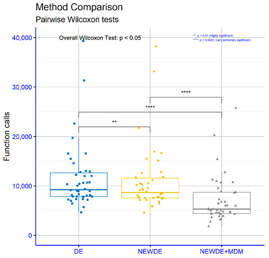
Figure 1.
Statistical comparison of classic DE with new DE and new DE with majority dimension mechanism.
Table 3 and Figure 2 present a comparative performance analysis of various optimization methods, including GA, WOA, PSO, Ant Colony Optimization (ACO) [43], self-adaptive differential evolution (SaDE), and NEWDE + MDM. The NEWDE + MDM method demonstrates the best overall performance, with the lowest total number of function evaluations (332,921) and a high success rate (97%). Specifically, for functions such as ACKLAY (7249 evaluations), BF1 (5204), and GKLS350 (1811 evaluations with a 96% success rate), NEWDE + MDM clearly outperforms the other methods. Furthermore, its performance on complex functions like RASTRIGIN (4639 evaluations with a 93% success rate) and HARTMAN3 (3179 evaluations) is particularly impressive. The WOA shows the highest number of evaluations (1,098,519), indicating significantly higher computational costs compared to the other methods. However, its success rate remains high (98%), demonstrating that, despite its inefficiency, the algorithm can provide reliable results for certain problems. Both the GA and PSO show similar performance, with total evaluations of 335,162 and 350,871, respectively, and success rates of 99% and 98%. However, for specific functions like DIFFPOWER10, PSO appears to be slightly superior, while the GA performs better on functions like SHEKEL5 and SHEKEL7. The ACO algorithm shows the lowest success rate (80%) and a high evaluation count (406,302), making it less efficient compared to the other methods. Nevertheless, for certain functions like ELP10 (4637 evaluations) and GKLS250 (4459 evaluations), ACO can be competitive. The SaDE method demonstrates interesting results, with a total number of objective function evaluations (457,425) higher than NEWDE + MDM but lower than the WOA while maintaining a very high success rate (0.99), the highest among all the methods. This indicates that SaDE, while less efficient than NEWDE + MDM in terms of required function evaluations, offers exceptional reliability in finding the global minimum, particularly in complex optimization problems where convergence to local minima is a frequent pitfall. Overall, the results confirm that NEWDE + MDM is the most effective method, particularly for problems with multiple local minima and high dimensionality. While the other methods may be effective in specific cases, they cannot match the overall performance of NEWDE + MDM. This analysis highlights the importance of selecting the appropriate optimization algorithm based on the problem characteristics.

Figure 2.
Detailed comparison of methods for each optimization problem.
The results of the statistical analysis (Friedman test [44]) conducted in R for comparing various optimization methods revealed significant differences in their performance (Figure 3). Specifically, a very extremely significant difference (p < 0.0001) was observed between the GA and WOA, indicating that these two methods differ substantially in terms of performance. However, comparisons between the GA and PSO as well as the GA and ACO showed non-significant differences (p > 0.05), meaning their performances are statistically indifferent. The comparison between the GA and SaDE showed a significant difference (p < 0.05), suggesting that SaDE performs differently compared to the genetic algorithm. In contrast, the comparison between the WOA and PSO showed no significant difference (p > 0.05), while the WOA versus ACO again showed a very extremely significant difference (p < 0.0001). Furthermore, the WOA differs significantly (p < 0.05) from SaDE, but this difference becomes highly significant (p < 0.01) when examined in another context. The comparison between the WOA and the modified differential evolution (NEWDE + MDM) showed a very extremely significant difference (p < 0.0001), confirming the superiority of the latter method. The comparisons between PSO and ACO, as well as between ACO and NEWDE + MDM, showed non-significant differences (p > 0.05). However, PSO differs significantly (p < 0.05) from SaDE, as does ACO when compared to SaDE. Finally, the comparison between SaDE and the WOA confirms an extremely significant difference (p < 0.001), highlighting that SaDE has statistically better performance compared to the WOA. Overall, the results demonstrate that NEWDE + MDM stands out for its superior performance compared to the other methods, while the WOA shows large statistical differences relative to most of the other techniques. These findings can help in selecting the optimal method depending on the optimization problem at hand.
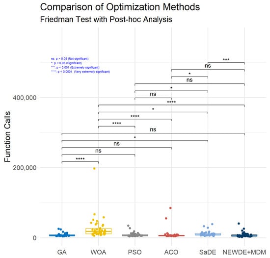
Figure 3.
Statistical comparison of new DE with majority dimension mechanism method versus others.
Table 5 presents a detailed comparison of various termination criteria for the proposed optimization algorithm, including BSS, WSS, TSS, BOSS, SRS, IRS, doublebox, and the combined “All” criterion that incorporates all the previous rules. The analysis reveals that the IRS criterion achieves the lowest total number of function evaluations (263,582) with a 96% success rate, making it the most efficient among the individual termination rules. The “All” criterion, which combines all the rules, demonstrates similar performance, with 257,860 evaluations and a 96% success rate, confirming the superiority of this combined approach. In contrast, the BOSS criterion requires the highest number of evaluations (1,318,249) despite its excellent success rate (99%). This indicates that, while BOSS reliably finds the global optimum, it does so at a significantly increased computational cost. Similarly, the TSS and SRS criteria also require relatively high evaluation counts (465,279 and 420,140, respectively). For specific test functions like GKLS350, all the termination criteria achieve high success rates (96%), with IRS and “All” requiring the fewest evaluations (1811). For the RASTRIGIN function, IRS and “All” stand out with 3548 evaluations and a 93% success rate compared to BOSS, requiring 15,210 evaluations. Similarly, for HARTMAN3, the BSS, IRS, and All criteria need the fewest evaluations (3179, 3042, and 2651, respectively). In cases like POTENTIAL6, the doublebox criterion achieves the highest success rate (96%) but requires substantially more evaluations (35,090) compared to IRS (9616), which has a lower success rate (70%). This demonstrates the need to balance accuracy against computational cost. Overall, the results confirm that either combining multiple criteria (“All”) or using IRS provides the best balance between reduced function evaluations and high success rates. Conversely, criteria like BOSS, while reliable, significantly increase the computational burden. The optimal termination rule selection depends on the problem requirements, particularly regarding the trade-off between solution accuracy and computational efficiency.
Table 5.
The proposed method with new different stopping rules.
The results of the statistical analysis conducted to compare various termination rules revealed interesting findings regarding the statistical significance of their differences (Figure 4). Specifically, the comparison between the BSS (Best Solution Stopping) and WSS (Worst Solution Stopping) rules showed no significant difference (p > 0.05), indicating that these two termination approaches do not differ significantly in terms of their effectiveness. Similarly, non-significant differences were observed in comparisons between BSS and TSS (Total Solution Stopping), SRS (Solution Range Stopping), IRS (Iteration Range Stopping), doublebox, and “All”. However, the comparison between BSS and BOSS (Best Overall Solution Stopping) showed an extremely significant difference (p < 0.001), suggesting that the BOSS rule differs significantly from BSS. A similar, although less statistically significant, difference was observed between WSS and BOSS (p < 0.05). Notable differences were observed in the other comparisons. The TSS vs. IRS comparison showed a highly significant difference (p < 0.01), while TSS vs. “All” showed an extremely significant difference (p < 0.001). The differences between BOSS and IRS, as well as between BOSS and "All", were very extremely significant (p < 0.0001 in both cases). Significant differences were also observed between SRS and IRS (p < 0.05), and between SRS and “All” (p < 0.001). Finally, the IRS vs. “All” comparison showed a very extremely significant difference (p < 0.0001), while the doublebox vs. “All” comparison also showed a very extremely significant difference (p < 0.0001). These findings highlight that certain termination rules, such as BOSS and "All", show statistically significant differences compared to other rules, which may have important implications for selecting the optimal termination rule for different optimization problems.
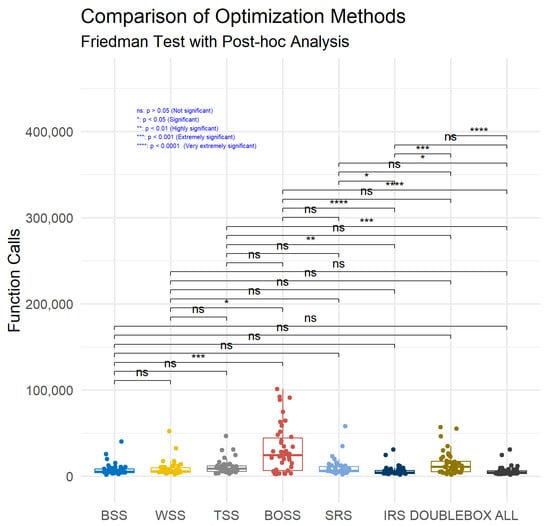
Figure 4.
Statistical comparison of NEWDE + MDM with different stopping rules.
4. Discussion of Findings and Comparative Analysis
The NEWDE algorithm is an enhanced version of the classical differential evolution algorithm, designed to address the core challenges of the conventional optimization methods, such as premature convergence and the inability to balance the exploration and exploitation of the solution space. The key improvement lies in the use of a dual mutation strategy, which enables a more flexible approach. The addition of the majority dimension mechanism to NEWDE makes it even more efficient. The experimental results showed that NEWDE + MDM reduced the number of required objective function evaluations by an average of 30% compared to classical DE. In specific cases, such as the GKLS350 function, the reduction was even more impressive, from 8107 to just 1811 evaluations, while maintaining a high success rate (96%). This improvement is primarily due to the dynamic balance the algorithm achieves between the exploration and exploitation of the search space. The new termination rules, particularly IRS and the combined “All” criterion, proved to be highly effective. For example, in the Rastrigin function, the IRS rule delivered the best results, with only 3548 evaluations and a 93% success rate, whereas the BOSS rule required significantly more computations (15,210 evaluations) despite having a slightly higher success rate (99%). The statistical analysis confirmed that NEWDE + MDM performs significantly better than other popular methods, such as genetic algorithms and Particle Swarm Optimization. Specifically, the results of the Friedman test validated the superiority of NEWDE + MDM, particularly in high-dimensional problems like POTENTIAL10, where the evaluations decreased from 197,044 (with WOA) to 20,237.
Compared to recent self-adaptive variants of differential evolution, such as jDE and SaDE, the proposed method retains the structural simplicity of classical DE while introducing two targeted mutation strategies. Strategy 1 enhances exploration by directing individuals away from the current global best solution, thus promoting diversity, whereas Strategy 2 intensifies exploitation through adaptive differential variation involving multiple individuals. In contrast, jDE focuses on the self-adaptive control of the algorithmic parameters (F and CR) at the individual level, while SaDE further incorporates adaptive selection among different mutation strategies based on historical performance. The proposed method does not dynamically adapt parameters or strategies but instead applies a fixed yet flexible design that balances exploration and exploitation. Furthermore, unlike hybrid DE models, which integrate external metaheuristics, this approach remains “pure” in terms of its DE foundation. It introduces internal refinements without significantly increasing the algorithmic complexity. This design aims to preserve computational efficiency and maintain a lightweight framework, which has been recognized as a key advantage in the large-scale use of DE.
Despite these positive results, the algorithm has some limitations. Its performance on dynamic problems, where parameters change over time, remains an open challenge. Additionally, the need for specialized parameter tuning may pose a barrier for non-expert users. Future work could focus on automated parameter tuning using machine learning techniques and the development of parallel versions of the algorithm for greater computational efficiency.
5. Conclusions and Future Research Directions
This study presents a modified differential evolution algorithm designed to overcome the limitations of the traditional versions, offering improved performance in complex optimization problems. The results demonstrate that the proposed algorithm achieves significantly higher solution quality and greater efficiency, particularly in high-dimensional problems or those with multiple local minima. A key improvement mechanism is the introduction of a dual mutation strategy that operates in two distinct ways. The first approach focuses on exploring the search space, encouraging the algorithm to investigate unstudied regions. This is achieved by using distances from the best solution and applying random coefficients to create new points. The second approach prioritizes exploiting promising areas of the search space, where differential coefficients are dynamically adjusted based on data from multiple solutions.
The majority dimension mechanism adds a new dimension to the algorithm’s adaptability. Through dimension-wise analysis, it compares candidate solutions against two key reference points: the best and worst samples. This approach enables the algorithm to decide whether to focus on an intensive search around a promising region or explore new unknown areas of the space. The MDM prevents stagnation in local minima and enables the discovery of solutions that would otherwise remain unknown.
The new termination rules represent another innovation that enhances the overall algorithm performance. These rules are based on multidimensional metrics assessing the solution homogeneity and stability at various levels. For instance, the stability of the best solution, evolution of worst solutions, and overall convergence of the value ranges within the population indicate when the search is sufficiently complete. These rules reduce unnecessary computations while ensuring termination only when the highest possible solution quality is achieved.
In the experimental results, the NEWDE + MDM algorithm showed significant improvement over classical DE. For the GKLS350 function, the required computations decreased from 8107 to just 1811, with a 96% success rate. Similarly, for the Rastrigin function, the IRS termination rule required only 3548 computations (93% success) versus the BOSS rule’s 15,210 computations (99% success). For DIFFPOWER5, NEWDE + MDM recorded 25,736 computations versus NEWDE’s 33,168 and classical DE’s 31,332 (95% success). The HARTMAN6 function saw the computations reduced from 7181 to 4790 while maintaining 100% success. Particularly impressive were the results on multimodal functions like SHEKEL10, where NEWDE + MDM achieved solutions with only 5120 computations versus classical DE’s 8306, improving the success rate from 92% to 98%. For the high-dimensional ELP30 function, the computations decreased from 13,003 to 10,957 (97% success). On POTENTIAL10, the computations dropped from 197,044 (with WOA) to 20,237, while ROSENBROCK16 saw a reduction from 16,527 to 15,377 computations. For the challenging TEST2N7 function with multiple local minima, NEWDE + MDM produced solutions with 4565 computations (70% success) versus classical DE’s 12,006 computations (56% success). The statistical analysis showed that NEWDE + MDM achieved a statistically significant improvement (p < 0.05) in both computation count and success rate for 32 of the 38 test functions. The average computation reduction across all the functions was 31.7%, with the maximum reduction reaching 77.6% for GKLS350.
However, the research revealed certain limitations. A major challenge is the increased need for specialized parameter tuning as multiple strategy and termination rule choices may complicate use by non-experts. Additionally, the performance may decline in dynamic problems where characteristics change over time. Future research could focus on developing versions for dynamic problems, automated parameter tuning using machine learning techniques, and creating parallel versions to reduce execution time. Applications in fields like genetic engineering, autonomous vehicles, and energy system optimization could extend the algorithm’s impact. Finally, extensive experimental analysis across various data types and complexity levels could improve the algorithm’s reliability and robustness.
Author Contributions
Conceptualization, V.C. and G.K.; methodology, I.G.T.; software, V.C. and A.M.G.; validation, V.C. and I.G.T.; formal analysis, V.C.; investigation, V.C.; resources, I.G.T.; data curation, G.K.; writing—original draft preparation, V.C.; writing—review and editing, I.G.T.; visualization, V.C.; supervision, I.G.T.; project administration, I.G.T.; funding acquisition, I.G.T. All authors have read and agreed to the published version of the manuscript.
Funding
This research has been financed by the European Union: Next Generation EU through the Program Greece 2.0 National Recovery and Resilience Plan, under the call RESEARCH–CREATE–INNOVATE, project name “iCREW: Intelligent small craft simulator for advanced crew training using Virtual Reality techniques” (project code: TAEDK-06195).
Data Availability Statement
The original contributions presented in this study are included in the article. Further inquiries can be directed to the corresponding author.
Conflicts of Interest
The authors declare no conflicts of interest.
References
- Tapkir, A. A comprehensive overview of gradient descent and its optimization algorithms. Int. Res. J. Sci. Eng. Technol. 2023, 10, 37–45. [Google Scholar] [CrossRef]
- Cawade, S.; Kudtarkar, A.; Sawant, S.; Wadekar, H. The Newton-Raphson Method: A Detailed Analysis. Int. J. Res. Appl. Sci. Eng. (IJRASET) 2024, 12, 729–734. [Google Scholar] [CrossRef]
- Luenberger, D.G.; Ye, Y.; Luenberger, D.G.; Ye, Y. Interior-point methods. In Linear and Nonlinear Programming; Springer: Berlin/Heidelberg, Germany, 2021; pp. 129–164. [Google Scholar]
- Nemirovski, A.S.; Todd, M.J. Interior-point methods for optimization. Acta Numer. 2008, 17, 191–234. [Google Scholar] [CrossRef]
- Lam, A. Bfgs in a Nutshell: An Introduction to Quasi-Newton Methods; Towards Data Science: San Francisco, CA, USA, 2020. [Google Scholar]
- Sohail, A. Genetic algorithms in the fields of artificial intelligence and data sciences. Ann. Data Sci. 2023, 10, 1007–1018. [Google Scholar] [CrossRef]
- Deng, W.; Shang, S.; Cai, X.; Zhao, H.; Song, Y.; Xu, J. An improved differential evolution algorithm and its application in optimization problem. Soft Comput. 2021, 25, 5277–5298. [Google Scholar] [CrossRef]
- Pant, M.; Zaheer, H.; Garcia-Hernandez, L.; Abraham, A. Differential Evolution: A review of more than two decades of research. Eng. Appl. Artif. Intell. 2020, 90, 103479. [Google Scholar]
- Charilogis, V.; Tsoulos, I.G.; Tzallas, A.; Karvounis, E. Modifications for the differential evolution algorithm. Symmetry 2022, 14, 447. [Google Scholar] [CrossRef]
- Charilogis, V.; Tsoulos, I.G. A parallel implementation of the differential evolution method. Analytics 2023, 2, 17–30. [Google Scholar] [CrossRef]
- Shami, T.M.; El-Saleh, A.A.; Alswaitti, M.; Al-Tashi, Q.; Summakieh, M.A.; Mirjalili, S. Particle swarm optimization: A comprehensive survey. IEEE Access 2022, 10, 10031–10061. [Google Scholar] [CrossRef]
- Gad, A.G. Particle swarm optimization algorithm and its applications: A systematic review. Arch. Comput. Eng. 2022, 29, 2531–2561. [Google Scholar] [CrossRef]
- Abualigah, L.; Yousri, D.; Abd Elaziz, M.; Ewees, A.A.; Al-Qaness, M.A.; Gandomi, A.H. Aquila optimizer: A novel meta-heuristic optimization algorithm. Comput. Ind. Eng. 2021, 157, 107250. [Google Scholar] [CrossRef]
- Abualigah, L.; Sbenaty, B.; Ikotun, A.M.; Zitar, R.A.; Alsoud, A.R.; Khodadadi, N.; Jia, H. Aquila optimizer: Review, results and applications. Metaheuristic Optim. Algorithms 2024, 89–103. [Google Scholar] [CrossRef]
- Abualigah, L.; Diabat, A.; Mirjalili, S.; Abd Elaziz, M.; Gandomi, A.H. The arithmetic optimization algorithm. Comput. Methods Appl. Mech. Eng. 2021, 376, 113609. [Google Scholar] [CrossRef]
- Kaveh, A.; Hamedani, K.B. Improved arithmetic optimization algorithm and its application to discrete structural optimization. In Structures; Elsevier: Amsterdam, The Netherlands, 2022; Volueme 35, pp. 748–764. [Google Scholar]
- Zhang, J.; Zhang, G.; Huang, Y.; Kong, M. A novel enhanced arithmetic optimization algorithm for global optimization. IEEE Access 2022, 10, 75040–75062. [Google Scholar] [CrossRef]
- Eglese, R.W. Simulated annealing: A tool for operational research. Eur. J. Oper. Res. 1990, 46, 271–281. [Google Scholar] [CrossRef]
- Siarry, P.; Berthiau, G.; Durdin, F.; Haussy, J. Enhanced simulated annealing for globally minimizing functions of many-continuous variables. ACM Trans. Math. (TOMS) 1997, 23, 209–228. [Google Scholar] [CrossRef]
- Liu, Y.; Tian, P. A multi-start central force optimization for global optimization. Appl. Soft Comput. 2015, 27, 92–98. [Google Scholar] [CrossRef]
- Doumari, S.A.; Givi, H.; Dehghani, M.; Malik, O.P. Ring toss game-based optimization algorithm for solving various optimization problems. Int. J. Intell. Eng. Syst. 2021, 14, 545–554. [Google Scholar] [CrossRef]
- Salawudeen, A.T.; Mu’azu, M.B.; Yusuf, A.; Adedokun, A.E. A Novel Smell Agent Optimization (SAO): An extensive CEC study and engineering application. Knowl.-Based Syst. 2021, 232, 107486. [Google Scholar] [CrossRef]
- Salawudeen, A.T.; Mu’azu, M.B.; Sha’aban, Y.A.; Adedokun, E.A. On the development of a novel smell agent optimization (SAO) for optimization problems. In Proceedings of the 2nd International Conference on Information and Communication Technology and its Applications (ICTA 2018), Minna, Nigeria, 5–6 September 2018. [Google Scholar]
- Salawudeen, A.T.; Mu’azu, M.B.; Yusuf, A.; Adedokun, E.A. From smell phenomenon to smell agent optimization (SAO): A feasibility study. In Proceedings of the ICGET, Amsterdam, The Netherlands, 10–12 July 2018. [Google Scholar]
- Meadows, O.A.; Mu’Azu, M.B.; Salawudeen, A.T. A smell agent optimization approach to capacitated vehicle routing problem for solid waste collection. In Proceedings of the 2022 IEEE Nigeria 4th International Conference on Disruptive Technologies for Sustainable Development (NIGERCON), Lagos, Nigeria, 5–7 April 2022; pp. 1–5. [Google Scholar]
- Nadimi-Shahraki, M.H.; Zamani, H.; Asghari Varzaneh, Z.; Mirjalili, S. A systematic review of the whale optimization algorithm: Theoretical foundation, improvements, and hybridizations. Arch. Comput. Methods Eng. 2023, 30, 4113–4159. [Google Scholar] [CrossRef]
- Brodzicki, A.; Piekarski, M.; Jaworek-Korjakowska, J. The whale optimization algorithm approach for deep neural networks. Sensors 2021, 21, 8003. [Google Scholar] [CrossRef] [PubMed]
- Pourpanah, F.; Wang, R.; Lim, C.P.; Wang, X.Z.; Yazdani, D. A review of artificial fish swarm algorithms: Recent advances and applications. Artif. Intell. Rev. 2023, 56, 1867–1903. [Google Scholar] [CrossRef]
- Zhang, C.; Zhang, F.M.; Li, F.; Wu, H.S. Improved artificial fish swarm algorithm. In Proceedings of the 2014 9th IEEE Conference on Industrial Electronics and Applications, Hangzhou, China, 9–11 June 2014; pp. 748–753. [Google Scholar]
- Qin, A.K.; Suganthan, P.N. Self-adaptive differential evolution algorithm for numerical optimization. In Proceedings of the IEEE Congress on Evolutionary Computation, Edinburgh, UK, 2–5 September 2005. [Google Scholar] [CrossRef]
- Brest, J.; Zamuda, A.; Boskovic, B.; Sepesy, M.S.; Zumer, V. Dynamic optimization using self-adaptive differential evolution. In Proceedings of the IEEE Congress on Evolutionary Computation, Trondheim, Norway, 18–21 May 2009; pp. 415–422. [Google Scholar] [CrossRef]
- Hansen, N.; Ostermeier, A. Adapting arbitrary normal mutation distributions in evolution strategies: The covariance matrix adaptation. In Proceedings of the IEEE International Conference on Evolutionary Computation (ICEC ’96), Nagoya, Japan, 20–22 May 1996; pp. 312–317. [Google Scholar] [CrossRef]
- Tizhoosh, H.R. Opposition-Based Learning: A New Scheme for Machine Intelligence. In Proceedings of the International Conference on Computational Intelligence for Modelling, Control and Automation (CIMCA 2005), International Conference on Intelligent Agents, Web Technologies and Internet Commerce (IAWTIC 2005), Vienna, Austria, 28–30 November 2005; pp. 695–701. [Google Scholar] [CrossRef]
- Lagaris, I.E.; Tsoulos, I.G. Stopping rules for box-constrained stochastic global optimization. Appl. Math. Comput. 2008, 197, 622–632. [Google Scholar] [CrossRef]
- Charilogis, V.; Tsoulos, I.G.; Gianni, A.M. Combining Parallel Stochastic Methods and Mixed Termination Rules in Optimization. Algorithms 2024, 17, 394. [Google Scholar] [CrossRef]
- Koyuncu, H.; Ceylan, R. A PSO based approach: Scout particle swarm algorithm for continuous global optimization problems. J. Comput. Des. Eng. 2019, 6, 129–142. [Google Scholar] [CrossRef]
- LaTorre, A.; Molina, D.; Osaba, E.; Poyatos, J.; Del Ser, J.; Herrera, F. A prescription of methodological guidelines for comparing bio-inspired optimization algorithms. Swarm Evol. Comput. 2021, 67, 100973. [Google Scholar] [CrossRef]
- Gaviano, M.; Kvasov, D.E.; Lera, D.; Sergeyev, Y.D. Algorithm 829: Software for generation of classes of test functions with known local and global minima for global optimization. ACM Trans. Math. Softw. (TOMS) 2003, 29, 469–480. [Google Scholar] [CrossRef]
- Jones, J.E. On the determination of molecular fields.—II. From the equation of state of a gas. Proceedings of the Royal Society of London. Ser. Contain. Pap. Math. Phys. Character 1924, 106, 463–477. [Google Scholar]
- Zabinsky, Z.B.; Graesser, D.L.; Tuttle, M.E.; Kim, G.I. Global optimization of composite laminates using improving hit and run. In Recent Advances in Global Optimization; Princeton University Press: Princeton, NJ, USA, 1992; pp. 343–368. [Google Scholar]
- Tsoulos, I.G.; Charilogis, V.; Kyrou, G.; Stavrou, V.N.; Tzallas, A. OPTIMUS: A Multidimensional Global Optimization Package. J. Open Source Softw. 2025, 10, 7584. [Google Scholar] [CrossRef]
- Wilcoxon, F. Individual Comparisons by Ranking Methods. Int. Biom. Soc. 1945, 1, 80–83. [Google Scholar] [CrossRef]
- Dorigo, M.; Maniezzo, V.; Colorni, A. Ant system: Optimization by a colony of cooperating agents. IEEE Trans. Syst. Man, Cybern. Part B (Cybern.) 1996, 26, 29–41. [Google Scholar] [CrossRef] [PubMed]
- Friedman, M. The use of ranks to avoid the assumption of normality implicit in the analysis of variance. J. Am. Stat. Assoc. 1937, 32, 675–701. [Google Scholar] [CrossRef]
Disclaimer/Publisher’s Note: The statements, opinions and data contained in all publications are solely those of the individual author(s) and contributor(s) and not of MDPI and/or the editor(s). MDPI and/or the editor(s) disclaim responsibility for any injury to people or property resulting from any ideas, methods, instructions or products referred to in the content. |
© 2025 by the authors. Licensee MDPI, Basel, Switzerland. This article is an open access article distributed under the terms and conditions of the Creative Commons Attribution (CC BY) license (https://creativecommons.org/licenses/by/4.0/).