Novel Results on Global Asymptotic Stability of Time-Delayed Complex Valued Bidirectional Associative Memory Neural Networks

Abstract

This study investigates the global asymptotic stability of hybrid bidirectional associative memory (BAM) complex-valued neural networks (CVNNs) with time-varying delays and uncertain parameters, where the system matrices are assumed to be symmetric. By constructing an appropriate Lyapunov–Krasovskii functional (LKF), new sufficient conditions are derived to guarantee the existence and uniqueness of equilibrium points, as well as to establish the global asymptotic stability of the proposed symmetric hybrid BAM CVNNs. The validity and effectiveness of the theoretical results are further demonstrated through detailed numerical examples.

1. Introduction

Over the last few decades, neural networks (NNs) have gained substantial prominence as nonlinear circuit systems owing to their wide-ranging applications. Researchers have developed numerous NN architectures, including bidirectional associative memory (BAM) networks, Cohen–Grossberg networks, cellular neural networks, recurrent networks, and Hopfield networks. Among these, the BAM model—originally proposed by B. Kosko in 1987 [1]—stands out as a pivotal framework. It comprises two interconnected layers, referred to as the U-layer and the V-layer, which consist of hetero-associative neurons. These layers send signals back and forth to each other, allowing the BAM network to successfully handle tasks like storing memories and retrieving related information. Due to these features, BAM neural networks have been widely applied in fields such as pattern recognition, associative memory systems, and control automation. The dynamic behavior of BAM models continues to attract scholarly attention, particularly with respect to their stability properties. One of the foundational aspects influencing the behavior of neural networks is the presence and nature of equilibrium points. The stability of these points plays a crucial role in determining the overall system dynamics. Many researchers have explored different stability concepts such as global asymptotic stability, complete stability, and exponential stability—specifically for delayed neural systems, as indicated in the following references [2,3,4,5,6,7]. Recent studies on the stability of time-delayed neural networks have revealed many results, especially using Lyapunov’s theory and nonsmooth analytical methods. As a result, making sure that neural networks with delays remain stable over time and creating good control methods for them have become important research topics. This domain has only recently begun to gain widespread attention from the scientific community [8,9,10]. The concept of a new method for the stability analysis of nonlinear discrete-time systems and the stability analysis of layered digital dynamic networks using dissipativity theory was discussed in [11,12]. A substantial volume of work has explored topics including global asymptotic and stochastic stability, state estimation, and various stabilization mechanisms. Several studies have focused specifically on complex-valued recurrent neural networks (CVRNNs) with time delays [13,14,15,16,17,18,19,20]. For example, [21] showed how M-matrix theory can be used to study the overall stability of these systems, and the ideas of boundedness and complete stability were discussed in [22]. The issue of exponential stability with delays in CVRNNs was discussed in [20], and the existence, uniqueness, and exponential stability of memristor-based BAM neural networks with delays were studied in [19]. Additionally, researchers have looked into how stable fractional-order single-neuron models with delays are and how they behave during Hopf bifurcation [23]. The idea of Lagrange exponential stability for BAM-type complex-valued neural networks (CVNNs) with changing delays has also been thoroughly examined [24,25]. The concept of Lagrange exponential stability for BAM-type CVNNs with time-varying delays has also been studied in depth [24,25]. More recently, research on global $\mu$-stabilization for quaternion-valued inertial BAM neural networks incorporating time-varying delays via impulsive control has been presented in [26,27]. Also, a lot of focus has been given to making sure that discrete-time BAM networks remain globally exponentially stable even when they are influenced by impulses and delays, as shown in studies like [7,28,29,30].

Complex-valued BAM neural networks have recently gained more attention due to their importance in processing tasks with complex-valued signals. Unlike traditional real-valued networks, these systems contain complex numbers in their state variables, connection weights, or activation functions, resulting in richer and more complicated dynamics. Given these unique properties, it is crucial to study the dynamical properties of complex-valued BAM neural networks in more detail. An important theoretical problem in this area arises from a well-known result in complex analysis, Liouville’s theorem, which states that any function that is both bounded and complete (i.e., analytic everywhere) must be constant in the entire complex plane. This theorem highlights a fundamental limitation: activation functions in complex-valued neural networks cannot simultaneously satisfy both boundedness and analyticity. Therefore, selecting appropriate activation functions becomes a non-trivial task. A range of activation functions have been proposed for use in the complex domain. We have made significant progress in analyzing the dynamic behaviors of those activation functions that permit decomposition into separate real and imaginary components. In contrast, when such separation is not feasible, analysis has relied on the assumption that activation functions are globally Lipschitz continuous within the complex domain. This condition ensures tractability in studying system dynamics even in the absence of a clear decomposition. As a result, creating strong and effective neural network models in complicated areas needs to include specific features that help them handle to these limitations.

Based on the concepts and motivations mentioned above, the main contributions of this paper are summarized as follows.

• This study investigates the global asymptotic stability of complex-valued BAM neural networks containing multiple time-varying delays, commonly encountered in real-world signal processing and neurodynamic systems;
• The primary aim is to establish a new set of sufficient criteria that guarantee both the existence and uniqueness of equilibrium points while also confirming the global asymptotic stability of the proposed hybrid complex-valued BAM neural network framework;
• To achieve this, we develop a well-constructed Lyapunov–Krasovskii functional, taking into account the delay-dependent properties and hybrid structure of the system;
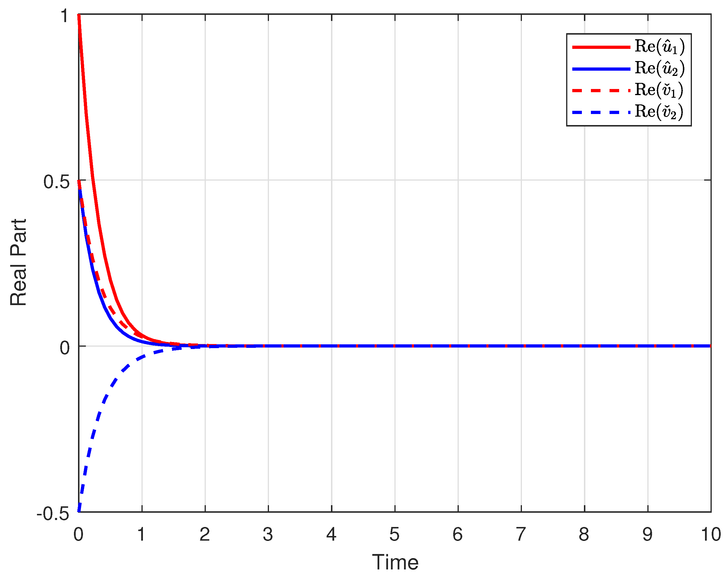
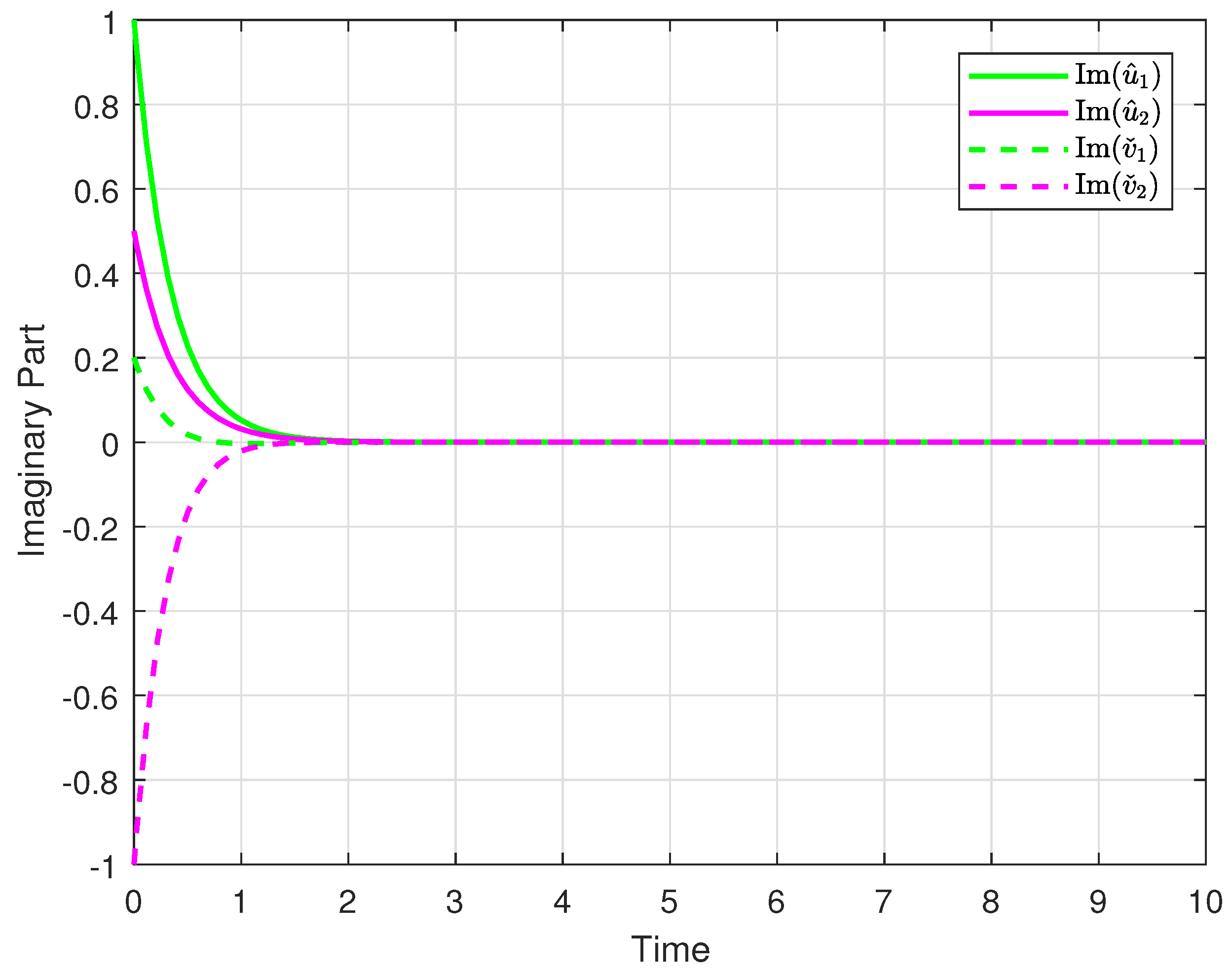
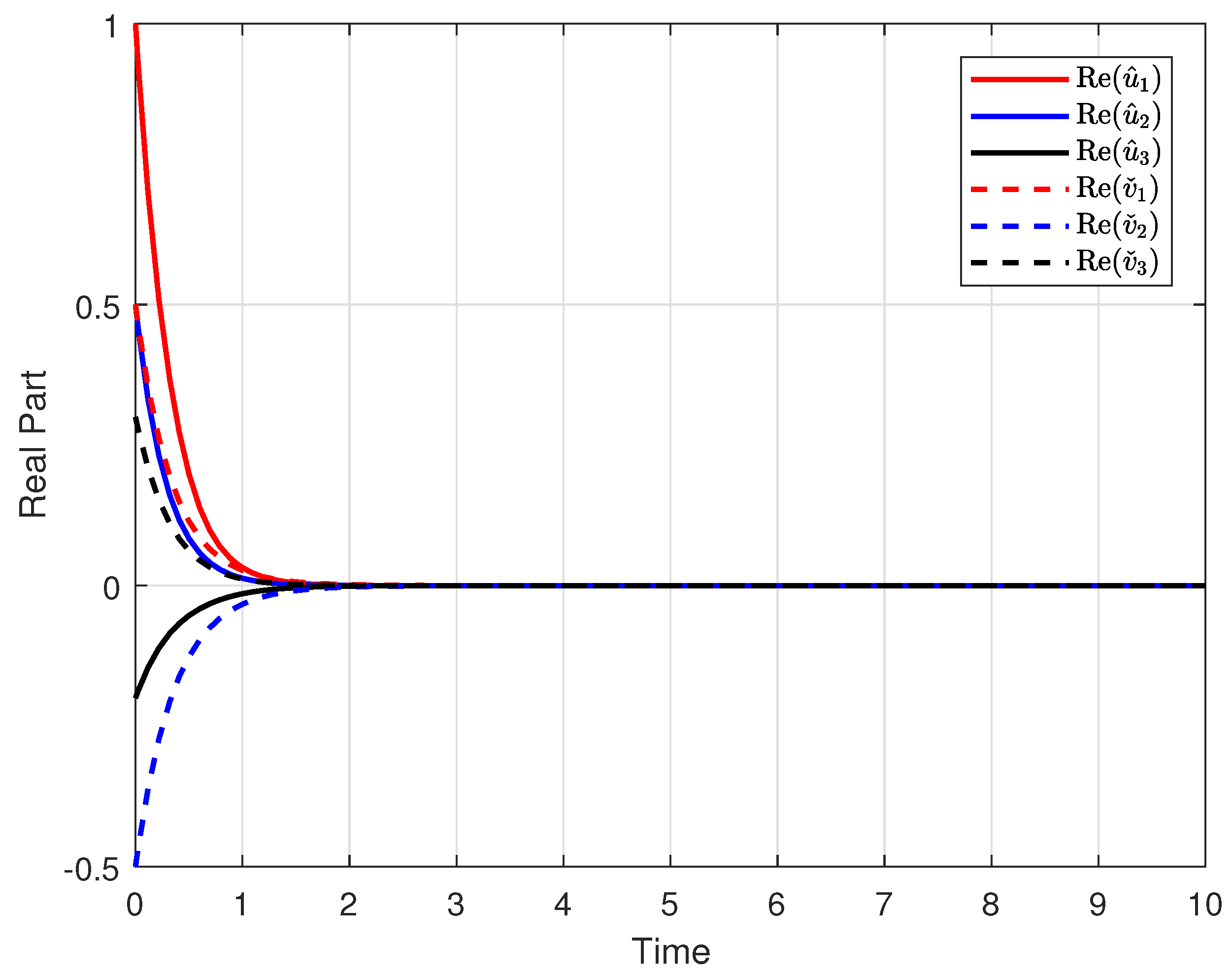
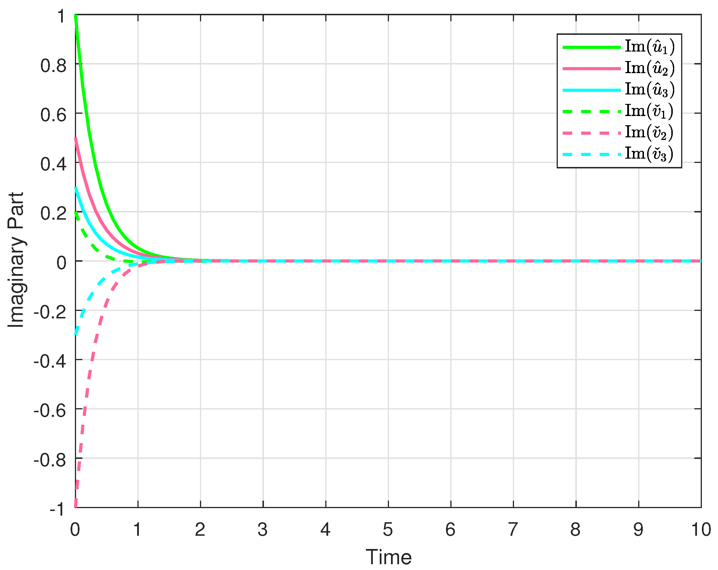
• Furthermore, carefully designed numerical simulations validate the theoretical results, demonstrating the effectiveness and practicality of the derived stability conditions.

Notations: The notations used in this manuscript are consistent with those in [15].

2. Preliminaries

Consider the system of hybrid complex-valued BAM NNs with time-varying delays:

$$\begin{array}{c}\hfill \left\{\begin{array}{cc}{\dot{w}}_i\left(t\right)=& -a_{ii}{w}_i\left(t\right)+\sum _{j=1}^m{b}_{ij}{\varphi }_j\left(z_j\left(t\right)\right)+\sum _{j=1}^m{c}_{ij}{\varphi }_j\left(z_j(t-\mathsf{\zeta }\left(t\right))\right)+J_i\left(t\right),\\ {\dot{z}}_j\left(t\right)=& -{\check{a}}_{jj}{z}_j\left(t\right)+\sum _{i=1}^n{\check{b}}_{ji}{\psi }_i\left(w_i\left(t\right)\right)+\sum _{i=1}^n{\check{c}}_{ji}{\psi }_i\left(w_i(t-\sigma \left(t\right))\right)+K_j\left(t\right),\end{array}\right.\end{array}$$

(1)

where $i=1,2,\cdots ,n,j=1,2,\cdots ,m$.

The following is the matrix form of (1):

$$\begin{array}{}\dot{w}\left(t\right)=-Aw\left(t\right)+B\mathsf{\Phi }\left(z\left(t\right)\right)+C\mathsf{\Phi }\left(z(t-\mathsf{\zeta }\left(t\right))\right)+J\left(t\right)\\ \dot{z}\left(t\right)=-\check{A}z\left(t\right)+\check{B}\mathsf{\Psi }\left(w\left(t\right)\right)+\check{C}\mathsf{\Psi }\left(w(t-\sigma \left(t\right))\right)+K\left(t\right),\end{array}$$

(2)

where $w\left(t\right)=(w_1\left(t\right),w_2\left(t\right),\cdots ,w_n\left(t\right))\in {\mathbb{C}}^n$ and $z\left(t\right)=(z_1\left(t\right),z_2\left(t\right),\cdots ,z_m\left(t\right))\in {\mathbb{C}}^m$ represent the state neurons at time t. $\mathsf{\Phi }\left(z(t-\mathsf{\zeta }\left(t\right))\right)={({\varphi }_1\left(z_1(t-{\mathsf{\zeta }}_1\left(t\right))\right),{\varphi }_2\left(z_2(t-{\mathsf{\zeta }}_2\left(t\right))\right),\cdots ,{\varphi }_m\left(z_m(t-{\mathsf{\zeta }}_m\left(t\right))\right))}^T\in {\mathbb{C}}^m$, $\mathsf{\Psi }\left(w(t-\sigma \left(t\right))\right)={({\psi }_1\left(w_1(t-{\sigma }_1\left(t\right))\right),{\psi }_2\left(w_2(t-{\sigma }_2\left(t\right))\right),\cdots ,{\psi }_m\left(w_n(t-{\sigma }_n\left(t\right))\right))}^T\in {\mathbb{C}}^n$ and $\mathsf{\Phi }\left(z(t-\mathsf{\zeta }\left(t\right))\right)={({\varphi }_1\left(z_1(t-{\mathsf{\zeta }}_1\left(t\right))\right),{\varphi }_2\left(z_2(t-{\mathsf{\zeta }}_2\left(t\right))\right),\cdots ,{\varphi }_m\left(z_m(t-{\mathsf{\zeta }}_m\left(t\right))\right))}^T\in {\mathbb{C}}^m$, $\mathsf{\Psi }\left(w\left(t\right)\right)={({\psi }_1\left(w_1\left(t\right)\right),{\psi }_2\left(w_2\left(t\right)\right),\cdots ,{\psi }_m\left(w_n\left(t\right)\right))}^T\in {\mathbb{C}}^n$ indicate neurons with and without time-varying delayed complex-valued activation functions, respectively; $A=diag[a_{11},a_{22},\cdots ,a_{nn}]\in {\mathbb{R}}^{n\times n}$, $\check{A}=diag[{\check{a}}_{11},{\check{a}}_{22},\cdots ,{\check{a}}_{mm}]\in {\mathbb{R}}^{m\times m}$ are the feedback connection matrices. $C={\left(c_{ij}\right)}_{n\times m}\in {\mathbb{C}}^{n\times m}$, $\check{C}={\left({\check{C}}_{ji}\right)}_{m\times n}\in {\mathbb{C}}^{m\times n}$ and $B={\left(b_{ij}\right)}_{n\times m}\in {\mathbb{C}}^{n\times m}$, $\check{B}={\left({\check{b}}_{ji}\right)}_{m\times n}\in {\mathbb{C}}^{m\times n}$ are the complex-valued connection matrices with and without time delays, respectively; $J\left(t\right)=(J_1\left(t\right),J2\left(t\right),\cdots ,J_n\left(t\right))\in {\mathbb{C}}^n$ and $K\left(t\right)=(K_1\left(t\right),K_2\left(t\right),\cdots ,K_m\left(t\right))\in {\mathbb{C}}^m$ are the external inputs.

In addition, the time-varying delays $\mathsf{\zeta }\left(t\right)$ and $\sigma \left(t\right)$ satisfy the following conditions

$$\begin{array}{}0\le \mathsf{\zeta }\left(t\right)\le {\mathsf{\zeta }}_1,\dot{\mathsf{\zeta }}\left(t\right)\le {\mathsf{\zeta }}_2<1\\ 0\le \sigma \left(t\right)\le {\sigma }_1,\dot{\sigma }\left(t\right)\le {\sigma }_2<1\end{array}$$

(3)

Several assumptions have been taken into account to find the stability of the system (1). In activation functions, the following assumptions will be taken for the entire research work: Suppose that $w_i=x_i+i{y}_i$ and $z_j={\widehat{x}}_j+i{\check{y}}_j$. Moreover, the activation functions ${\varphi }_i(.)$ and ${\psi }_j(.)$ $(·)$ are expressible as a combination of their real and imaginary parts:

$$\begin{array}{}{\varphi }_j\left(z_j\right)={\varphi }_j^R({\widehat{x}}_j,{\check{y}}_j)+i{\varphi }_j^I({\widehat{x}}_j,{\check{y}}_j)\\ {\psi }_i\left(w_i\right)={\psi }_i^R(x_i,y_i)+i{\psi }_i^I(x_i,y_i),\end{array}$$

where ${\varphi }_j^K:{\mathbb{R}}^2\to \mathbb{R}$, ${\psi }_j^K:{\mathbb{R}}^2\to \mathbb{R}$, $\forall K=R,I$.

Assumption A1.

$\left(A1\right)$. Assume that there are positive constants ${\eta }_j^{KR},{\eta }_j^{KI}$ and ${\nu }_i^{KR},{\nu }_i^{KI}$ for which the partial derivatives of ${\varphi }_j^K$ and ${\psi }_i^K$ with respect to $x_j,y_j$ and ${\widehat{x}}_j,{\check{y}}_j$ exist, respectively, and which are continuous, bounded, i.e.,

$$\begin{array}{c}\hfill |{\displaystyle \frac{\partial {\varphi }_j^K}{\partial x_j}}|\le {\eta }_j^{KR},|{\displaystyle \frac{\partial {\varphi }_j^K}{\partial y_j}}|\le {\eta }_j^{KI},|{\displaystyle \frac{\partial {\psi }_i^K}{\partial {\check{y}}_i}}|\le {\nu }_i^{KR},|{\displaystyle \frac{\partial {\psi }_i^K}{\partial {\widehat{x}}_i}}|\le {\nu }_i^{KI}\end{array}$$

for all $x_j,y_j,{\widehat{x}}_i,{\check{y}}_i\in \mathbb{R},K=R,I$.

Assumption A2.

$\left(A2\right)$. The following conditions are satisfied:

$$\begin{array}{c}\hfill |{\varphi }_j^K(x_j-x_j^{\prime })-{\varphi }_j^K(y_j-y_j^{\prime })|\le {\eta }_j^{KR}|x_j-x_j^{\prime }|+{\eta }_j^{KI}|y_j-y_j^{\prime }|,\\ \hfill |{\psi }_i^K({\widehat{x}}_i-{\widehat{x}}_i^{\prime })-{\psi }_i^K({\check{y}}_i-{\check{y}}_i^{\prime })|\le {\nu }_i^{KR}|{\widehat{x}}_i-{\widehat{x}}_i^{\prime }|+{\nu }_i^{KI}|{\check{y}}_i-{\check{y}}_i^{\prime }|,\end{array}$$

where $x_j,x_j^{\prime },y_j,y_j^{\prime },{\widehat{x}}_i,{\widehat{x}}_i^{\prime },{\check{y}}_i,{\check{y}}_i^{\prime }\in \mathbb{R}$, and $x_j\ne x_j^{\prime }$, $y_j\ne y_j^{\prime }$, ${\widehat{x}}_i\ne {\check{x}}_i^{\prime },{\check{y}}_i\ne {\check{y}}_i^{\prime }$,

Assumption A3.

$\left(A3\right)$. The following is the separation of the external inputs of (1) into real and imaginary parts: $J_i\left(t\right)=J_i^R\left(t\right)+i{J}_i^I\left(t\right),K_j\left(t\right)=K_j^R\left(t\right)+i{K}_j^I\left(t\right)$. In addition, the external inputs are bounded and satisfy $|J_i^R\left(t\right)|\le J_i^R,|J_i^I\left(t\right)|\le J_i^I,|K_j^R\left(t\right)|\le K_j^R,\left|K_j^I\left(t\right)\right|\le K_j^I$.

The system in (1) is reformulated by shifting its equilibrium point to the origin via the transformation given below:

$$\begin{array}{c}\hfill {\check{v}}_j(·)=z_j(·)-z_j^{*},{\widehat{u}}_i(·)=w_i(·)-w_i^{*},\forall i,j.\end{array}$$

Applying the above transformation, the system in (1) is reformulated as follows:

$$\left\{\begin{array}{cc}{\displaystyle \frac{d{\widehat{u}}_i\left(t\right)}{dt}}=& -a_{ii}{\widehat{u}}_i\left(t\right)+\sum _{j=i}^m{b}_{ij}{\chi }_{2j}\left({\check{v}}_j\left(t\right)\right)+\sum _{j=i}^m{c}_{ij}{\chi }_{2j}\left({\check{v}}_j(t-{\mathsf{\zeta }}_1)\right),\\ {\displaystyle \frac{d{\check{v}}_j\left(t\right)}{dt}}=& -{\check{a}}_{jj}{\check{v}}_j\left(t\right)+\sum _{i=i}^n{\check{b}}_{ji}{\chi }_{1i}\left({\widehat{u}}_i\left(t\right)\right)+\sum _{i=i}^n{\check{c}}_{ji}{\chi }_{1i}\left({\widehat{u}}_i(t-{\sigma }_1)\right),\end{array}\right.$$

(4)

where

$$\begin{array}{cc}\hfill i=& 1,2,\cdots ,n,j=1,2,\cdots ,m,{\chi }_{1i}\left({\widehat{u}}_i(·)\right)={\varphi }_i({\widehat{u}}_i(·)+w_i^{*})-{\varphi }_i\left(w_i^{*}\right),\hfill \\ \hfill {\chi }_{1i}\left(0\right)=& 0,{\chi }_{2j}\left({\check{v}}_j(·)\right)={\psi }_j({\check{z}}_j(·)+z_j^{*})-{\psi }_j\left(z_j^{*}\right),{\chi }_{2j}\left(0\right)=0,\forall i,j.\hfill \end{array}$$

The functions ${\chi }_{1i}$ and ${\chi }_{2j}$ satisfy the conditions for ${\varphi }_i$ and ${\psi }_j$, which means that ${\chi }_{1i},{\chi }_{2j}$ satisfy $\left(A1\right)$, $\left(A2\right)$, and $\left(A3\right)$. This can now be easily verified. Now, we separate the connection weight matrices into real and imaginary parts as follows:

$$\begin{array}{}B=B^R+i{B}^I={\left(b_{ij}^R\right)}_{n\times m}+i{\left(b_{ij}^I\right)}_{n\times m},\check{B}={\check{B}}^R+i{\check{B}}^I={\left({\check{b}}_{ji}^R\right)}_{m\times n}+i{\left({\check{b}}_{ji}^I\right)}_{m\times n},\\ C=C^R+i{C}^I={\left(c_{ij}^R\right)}_{n\times m}+i{\left(c_{ij}^I\right)}_{n\times m},\check{C}={\check{C}}^R+i{\check{C}}^I={\left({\check{c}}_{ji}^R\right)}_{m\times n}+i{\left({\check{c}}_{ji}^I\right)}_{m\times n}.\end{array}$$

The matrix form of (3) is expressed in the following manner:

$$\begin{array}{}\dot{\widehat{u}}\left(t\right)=-A\widehat{u}\left(t\right)+B{\chi }_2\left(\check{v}\left(t\right)\right)+C{\chi }_2\left(\check{v}(t-{\mathsf{\zeta }}_1)\right)\\ \dot{\check{v}}\left(t\right)=-\check{A}\check{v}\left(t\right)+\check{B}{\chi }_1\left(\widehat{u}\left(t\right)\right)+C{\chi }_2\left(\widehat{u}(t-{\sigma }_1)\right),\end{array}$$

(5)

where

$$\begin{array}{cc}\hfill \widehat{u}\left(t\right)=& {\widehat{x}}_1\left(t\right)+i{\check{y}}_1\left(t\right),\check{v}\left(t\right)={\widehat{x}}_2\left(t\right)+i{\check{y}}_2\left(t\right),\hfill \\ \hfill {\chi }_2\left(\check{v}\left(t\right)\right)=& {\chi }_2^R({\widehat{x}}_2\left(t\right),{\check{y}}_2\left(t\right))+i{\chi }_2^I({\widehat{x}}_2\left(t\right),{\check{y}}_2\left(t\right)),\hfill \\ \hfill {\chi }_2\left(\check{v}(t-{\mathsf{\zeta }}_1)\right)=& {\chi }_2^R\left({\widehat{x}}_2((t-{\mathsf{\zeta }}_1),{\check{y}}_2\left((t-{\mathsf{\zeta }}_1)\right))\right)+i{\chi }_2^I\left({\widehat{x}}_2((t-{\mathsf{\zeta }}_1),{\check{y}}_2\left((t-{\mathsf{\zeta }}_1)\right))\right),\hfill \\ \hfill {\chi }_1\left(\widehat{u}\left(t\right)\right)=& {\chi }_1^R({\widehat{x}}_1\left(t\right),{\check{y}}_1\left(t\right))+i{\chi }_1^I({\widehat{x}}_1\left(t\right),{\check{y}}_1\left(t\right)),\hfill \\ \hfill {\chi }_1\left(\widehat{u}(t-{\mathsf{\zeta }}_1)\right)=& {\chi }_1^R({\widehat{x}}_1((t-{\mathsf{\zeta }}_1),{\check{y}}_1\left((t-{\mathsf{\zeta }}_1)\right))+i{\chi }_1^I({\widehat{x}}_1((t-{\mathsf{\zeta }}_1),{\check{y}}_1\left((t-{\mathsf{\zeta }}_1)\right)).\hfill \end{array}$$

At this point, the matrix form of the distinct real and imaginary components of (5) can be written as follows:

$$\begin{array}{cc}\hfill {\dot{\widehat{x}}}_1\left(t\right)=& -A{\widehat{x}}_1\left(t\right)+B^R{\chi }_2^R({\widehat{x}}_2\left(t\right),{\check{y}}_2\left(t\right))-B^I{\chi }_2^I({\widehat{x}}_2\left(t\right),{\check{y}}_2\left(t\right))+C^R{\chi }_2^R\left({\widehat{x}}_2(t-{\mathsf{\zeta }}_1),{\check{y}}_2(t-{\mathsf{\zeta }}_1)\right)\hfill \\ & -C^I{\chi }_2^I\left({\widehat{x}}_2(t-{\mathsf{\zeta }}_1),{\check{y}}_2(t-{\mathsf{\zeta }}_1)\right),\hfill \end{array}$$

(6)

$$\begin{array}{cc}\hfill {\dot{\check{y}}}_1\left(t\right)=& -A{\check{y}}_1\left(t\right)+B^R{\chi }_2^I({\widehat{x}}_2\left(t\right),{\check{y}}_2\left(t\right))+B^I{\chi }_2^R({\widehat{x}}_2\left(t\right),{\check{y}}_2\left(t\right))+C^R{\chi }_2^I({\widehat{x}}_2((t-{\mathsf{\zeta }}_1),{\check{y}}_2(t-{\mathsf{\zeta }}_1))\hfill \\ & -C^I{\chi }_2^R\left({\widehat{x}}_2(t-{\mathsf{\zeta }}_1),{\check{y}}_2(t-{\mathsf{\zeta }}_1)\right),\hfill \end{array}$$

(7)

$$\begin{array}{cc}\hfill {\dot{\widehat{x}}}_2(t)=& -\check{A}{\widehat{x}}_2(t)+{\check{B}}^R{\chi }_1^R({\widehat{x}}_1(t),{\check{y}}_1(t))-{\check{B}}^I{\chi }_1^I({\widehat{x}}_1(t),{\check{y}}_1(t))+{\check{C}}^R{\chi }_1^R({\widehat{x}}_1(t-{\sigma }_1),{\check{y}}_1(t-{\sigma }_1))\hfill \\ & -{\check{C}}^I{\chi }_1^I({\widehat{x}}_1(t-{\sigma }_1),{\check{y}}_1(t-{\sigma }_1)),\hfill \end{array}$$

(8)

$$\begin{array}{cc}\hfill {\dot{\check{y}}}_2\left(t\right)=& -\check{A}{\check{y}}_2\left(t\right)+{\check{B}}^R{\chi }_1^I({\widehat{x}}_1\left(t\right),{\check{y}}_1\left(t\right))+{\check{B}}^I{\chi }_1^R({\widehat{x}}_1\left(t\right),{\check{y}}_1\left(t\right))+{\check{C}}^R{\chi }_1^I\left({\widehat{x}}_1(t-{\sigma }_1),{\check{y}}_1(t-{\sigma }_1)\right)\hfill \\ & -{\check{C}}^I{\chi }_1^R\left({\widehat{x}}_1(t-{\sigma }_1),{\check{y}}_1(t-{\sigma }_1)\right).\hfill \end{array}$$

(9)

Now, (6)–(9) can also be written as the following form:

$$\begin{array}{cc}\hfill {\dot{\widehat{x}}}_{1i}\left(t\right)=& -a_{ii}{\widehat{x}}_{1i}\left(t\right)+\sum _{j=1}^m{b}_{ij}^R{\chi }_{2j}^R({\widehat{x}}_{2j}\left(t\right),{\check{y}}_{2j}\left(t\right))-\sum _{j=1}^m{b}_{ij}^I{\chi }_{2j}^I({\widehat{x}}_{2j}\left(t\right),{\check{y}}_{2j}\left(t\right))\hfill \\ & +\sum _{j=1}^m{c}_{ij}^R{\chi }_{2j}^R({\widehat{x}}_{2j}(t-{\mathsf{\zeta }}_1),{\check{y}}_{2j}\left((t-{\mathsf{\zeta }}_1)\right)-\sum _{j=1}^m{c}_{ij}^I{\chi }_{2j}^I({\widehat{x}}_{2j}(t-{\mathsf{\zeta }}_1),{\check{y}}_{2j}(t-{\mathsf{\zeta }}_1)),\hfill \end{array}$$

(10)

$$\begin{array}{cc}\hfill {\dot{\check{y}}}_{1i}\left(t\right)=& -a_{ii}{\check{y}}_{1i}\left(t\right)+\sum _{j=1}^m{b}_{ij}^R{\chi }_{2j}^I({\widehat{x}}_{2j}\left(t\right),{\check{y}}_{2j}\left(t\right))+\sum _{j=1}^m{b}_{ij}^I{\chi }_{2j}^R({\widehat{x}}_{2j}\left(t\right),{\check{y}}_{2j}\left(t\right))\hfill \\ & +\sum _{j=1}^m{c}_{ij}^R{\chi }_{2j}^I({\widehat{x}}_{2j}(t-{\mathsf{\zeta }}_1),{\check{y}}_{2j}(t-{\mathsf{\zeta }}_1))+\sum _{j=1}^m{c}_{ij}^I{\chi }_{2j}^R({\widehat{x}}_{2j}(t-{\mathsf{\zeta }}_1),{\check{y}}_{2j}(t-{\mathsf{\zeta }}_1)),\hfill \end{array}$$

(11)

$$\begin{array}{cc}\hfill {\dot{\widehat{x}}}_{2j}\left(t\right)=& -{\check{a}}_{jj}{\widehat{x}}_{2j}\left(t\right)+\sum _{j=1}^m{\check{b}}_{ij}^R{\chi }_{1i}^R({\widehat{x}}_{1i}\left(t\right),{\check{y}}_{1i}\left(t\right))-\sum _{j=1}^m{\check{b}}_{ij}^I{\chi }_{1i}^I({\widehat{x}}_{1i}\left(t\right),{\check{y}}_{1i}\left(t\right))\hfill \\ & +\sum _{j=1}^m{\check{c}}_{ij}^R{\chi }_{1i}^R({\widehat{x}}_{1i}(t-{\sigma }_1),{\check{y}}_{1i}(t-{\sigma }_1))-\sum _{j=1}^m{\check{c}}_{ij}^I{\chi }_{1i}^I({\widehat{x}}_{1i}(t-{\sigma }_1),{\check{y}}_{1i}(t-{\sigma }_1)),\hfill \end{array}$$

(12)

$$\begin{array}{cc}\hfill {\dot{\check{y}}}_{2j}\left(t\right)=& -{\check{a}}_{jj}{\check{y}}_{2j}\left(t\right)+\sum _{j=1}^m{\check{b}}_{ij}^R{\chi }_{1i}^I({\widehat{x}}_{1i}\left(t\right),{\check{y}}_{1i}\left(t\right))+\sum _{j=1}^m{\check{b}}_{ij}^I{\chi }_{1i}^R({\widehat{x}}_{1i}\left(t\right),{\check{y}}_{1i}\left(t\right))\hfill \\ & +\sum _{j=1}^m{\check{c}}_{ij}^R{\chi }_{1i}^I({\widehat{x}}_{1i}(t-{\sigma }_1),{\check{y}}_{1i}(t-{\sigma }_1))-\sum _{j=1}^m{\check{c}}_{ij}^I{\chi }_{1i}^R({\widehat{x}}_{1i}(t-{\sigma }_1),{\check{y}}_{1i}(t-{\sigma }_1)).\hfill \end{array}$$

(13)

Lemma 1.

The subsequent inequality is valid for any pair of vectors. $u={(u_1,u_2,\cdots ,u_n)}^T\in {\mathbb{C}}^n$ and $v={(v_1,v_2,\cdots ,v_n)}^T\in {\mathbb{C}}^n$, and a positive definite Hermitian matrix $D\in {\mathbb{C}}^{n\times n}$ is found:

$$\begin{array}{c}\hfill 2u^{*}v=2v^{*}u\le \beta u^{*}u+{\displaystyle \frac{1}{\beta }}{v}^{*}v,\forall \beta >0.\end{array}$$

3. Main Results

This section will establish some new sufficient conditions for the global asymptotic stability of (5) given the condition (3). Applying assumptions, the system represented by equation (5), which satisfies (3), has an equilibrium point. Therefore, it is crucial to establish the uniqueness and global asymptotic stability of the equilibrium point of (5) or an equivalent (1).

Theorem 1.

Assume that the activation functions ${\chi }_{1i},{\chi }_{2j}$ fulfill conditions $\left(A1\right),\left(A2\right)$ and that there are positive constants ${\alpha }_i,{\check{\alpha }}_j,{\beta }_i$ and ${\check{\beta }}_j$ such that the following conditions are satisfied:

$$\begin{array}{cc}\hfill {\Xi }_1=& mi{n}_{1\le i\le n}\{a_{ii}-\sum _{j=i}^n{\displaystyle \frac{{\check{\alpha }}_j}{{\alpha }_i}}\left[\right(|{\check{b}}_{ji}^R|+|{\check{c}}_{ji}^R\left|\right){\nu }_i^{RR}+\left(\right|{\check{b}}_{ji}^I|+|{\check{c}}_{ji}^I\left|\right){\nu }_i^{IR}]\hfill \\ \hfill -& \sum _{j=i}^n{\displaystyle \frac{{\check{\beta }}_j}{{\alpha }_i}}\left[\right(|{\check{b}}_{ji}^I|+|{\check{c}}_{ji}^I\left|\right){\nu }_i^{RR}+\left(\right|{\check{b}}_{ji}^R|+|{\check{c}}_{ji}^R\left|\right){\nu }_i^{IR}\left]\right\}>0,\hfill \\ \hfill {\Xi }_2=& mi{n}_{1\le i\le n}\{a_{ii}-\sum _{j=i}^n{\displaystyle \frac{{\check{\alpha }}_j}{{\beta }_i}}\left[\right(|{\check{b}}_{ji}^R|+|{\check{c}}_{ji}^R\left|\right){\nu }_i^{RI}+\left(\right|{\check{b}}_{ji}^I|+|{\check{c}}_{ji}^I\left|\right){\nu }_i^{II}]\hfill \\ \hfill -& \sum _{j=i}^n{\displaystyle \frac{{\check{\beta }}_j}{{\beta }_i}}\left[\right(|{\check{b}}_{ji}^R|+|{\check{c}}_{ji}^R\left|\right){\nu }_i^{II}+\left(\right|{\check{b}}_{ji}^I|+|{\check{c}}_{ji}^I\left|\right){\nu }_i^{RI}\left]\right\}>0,\hfill \\ \hfill {\Xi }_3=& mi{n}_{1\le j\le n}\{{\check{a}}_{jj}-\sum _{i=i}^n{\displaystyle \frac{{\alpha }_i}{{\check{\alpha }}_j}}\left[\right(|b_{ij}^R|+|c_{ij}^R\left|\right){\eta }_j^{RR}+\left(\right|b_{ij}^I|+|c_{ij}^I\left|\right){\eta }_j^{IR}]\hfill \\ \hfill -& \sum _{i=i}^n{\displaystyle \frac{{\beta }_i}{{\check{\alpha }}_j}}\left[\right(|b_{ij}^R|+|c_{ij}^R\left|\right){\eta }_j^{IR}+\left(\right|b_{ij}^I|+|c_{ij}^I\left|\right){\eta }_j^{RR}\left]\right\}>0,\hfill \\ \hfill {\Xi }_4=& mi{n}_{1\le j\le n}\{{\check{a}}_{jj}-\sum _{i=i}^n{\displaystyle \frac{{\alpha }_i}{{\check{\beta }}_j}}\left[\right(|b_{ij}^R|+|c_{ij}^R\left|\right){\eta }_j^{RI}+\left(\right|b_{ij}^I|+|c_{ij}^I\left|\right){\eta }_j^{II}]\hfill \\ \hfill -& \sum _{i=i}^n{\displaystyle \frac{{\beta }_i}{{\check{\beta }}_j}}\left[\right(|b_{ij}^R|+|c_{ij}^R\left|\right){\eta }_j^{II}+\left(\right|b_{ij}^I|+|c_{ij}^I\left|\right){\eta }_j^{RI}\left]\right\}>0,\hfill \end{array}$$

Then, (5) has a unique equilibrium point as its origin.

Proof. 

The unique equilibrium point of (5) will be demonstrated to be the origin using this theorem. Assume that the equilibrium points of (3) are ${({\widehat{u}}_1^{*},\dots ,{\widehat{u}}_n^{*})}^T={\widehat{u}}^{*}\ne 0$ and ${({\check{v}}_1^{*},...,{\check{v}}_m^{*})}^T={\check{v}}^{*}\ne 0$. The points that fulfill the following equations are (5)’s equilibrium points:

$$-a_{ii}{\widehat{u}}_i^{*}+\sum _{j=i}^m{b}_{ij}{\chi }_{2j}\left({\check{v}}_j^{*}\right)+\sum _{j=i}^m{c}_{ij}{\chi }_{2j}\left({\check{v}}_j^{*}\right)=0,\forall i,$$

(14)

$$-{\check{a}}_{jj}{\check{v}}_j^{*}+\sum _{i=i}^n{\check{b}}_{ji}{\chi }_{1j}\left({\widehat{u}}_i^{*}\right)+\sum _{i=i}^n{\check{c}}_{ji}{\chi }_{1j}\left({\widehat{u}}_i^{*}\right)=0,\forall j.$$

(15)

Equations (14) and (15) can be separated into the real and imaginary parts as follows:

$$\begin{array}{cc}\hfill & -a_{ii}{\widehat{x}}_{1i}^{*}+\sum _{j=i}^m{b}_{ij}^R{\chi }_{2j}^R({\widehat{x}}_{2j}^{*},{\check{y}}_{2j}^{*})-\sum _{j=i}^m{b}_{ij}^I{\chi }_{2j}^I({\widehat{x}}_{2j}^{*},{\check{y}}_{2j}^{*})\hfill \\ \hfill +& \sum _{j=i}^m{c}_{ij}^R{\chi }_{2j}^R({\widehat{x}}_{2j}^{*},{\check{y}}_{2j}^{*})-\sum _{j=i}^m{c}_{ij}^I{\chi }_{2j}^I({\widehat{x}}_{2j}^{*},{\check{y}}_{2j}^{*})=0,\forall i,\hfill \end{array}$$

(16)

$$\begin{array}{cc}\hfill -& a_{ii}{\check{y}}_{1i}^{*}+\sum _{j=1}^m{b}_{ij}^R{\chi }_{2j}^I({\widehat{x}}_{2j}^{*},{\check{y}}_{2j}^{*})+\sum _{j=1}^m{b}_{ij}^I{\chi }_{2j}^R({\widehat{x}}_{2j}^{*},{\check{y}}_{2j}^{*})\hfill \\ \hfill +& \sum _{j=1}^m{c}_{ij}^R{\chi }_{2j}^I({\widehat{x}}_{2j}^{*},{\check{y}}_{2j}^{*})+\sum _{j=1}^m{c}_{ij}^I{\chi }_{2j}^R({\widehat{x}}_{2j}^{*},{\check{y}}_{2j}^{*})=0,\forall i,\hfill \end{array}$$

(17)

$$\begin{array}{cc}\hfill & -{\check{a}}_{jj}{\widehat{x}}_{2j}^{*}+\sum _{j=1}^m{\check{b}}_{ij}^R{\chi }_{1i}^R({\widehat{x}}_{1i}^{*},{\check{y}}_{1i}^{*})-\sum _{j=1}^m{\check{b}}_{ij}^I{\chi }_{1i}^I({\widehat{x}}_{1i}^{*},{\check{y}}_{1i}^{*})\hfill \\ & +\sum _{j=1}^m{\check{c}}_{ij}^R{\chi }_{1i}^R({\widehat{x}}_{1i}^{*},{\check{y}}_{1i}^{*})-\sum _{j=1}^m{\check{c}}_{ij}^I{\chi }_{1i}^I({\widehat{x}}_{1i}^{*},{\check{y}}_{1i})=0,\forall j,\hfill \end{array}$$

(18)

$$\begin{array}{cc}\hfill & -{\check{a}}_{jj}{\check{y}}_{2j}^{*}+\sum _{j=1}^m{\check{b}}_{ij}^R{\chi }_{1i}^I({\widehat{x}}_{1i}^{*},{\check{y}}_{1i}^{*})+\sum _{j=1}^m{\check{b}}_{ij}^I{\chi }_{1i}^R({\widehat{x}}_{1i}^{*},{\check{y}}_{1i}^{*})\hfill \\ & +\sum _{j=1}^m{\check{c}}_{ij}^R{\chi }_{1i}^I({\widehat{x}}_{1i}^{*},{\check{y}}_{1i}^{*})+\sum _{j=1}^m{\check{c}}_{ij}^I{\chi }_{1i}^R({\widehat{x}}_{1i}^{*},{\check{y}}_{1i}^{*})=0,\forall j.\hfill \end{array}$$

(19)

The following equations are obtained by applying (A1) and (A2) in (16)–(19):

$$\begin{array}{cc}\hfill a_{ii}\left|{\widehat{x}}_{1i}^{*}\right|\le & \sum _{j=i}^m|b_{ij}^R|({\nu }_j^{RR}|{\widehat{x}}_{2j}^{*}|+{\nu }_j^{RI}|{\check{y}}_{2j}^{*}|)+\sum _{j=i}^m|b_{ij}^I|({\nu }_{2j}^{IR}|{\widehat{x}}_{2j}^{*}|+{\nu }_{2j}^{II}|{\check{y}}_{2j}^{*}|)\hfill \\ & +\sum _{j=i}^m|c_{ij}^R|({\nu }_j^{RR}|{\widehat{x}}_{2j}^{*}|+{\nu }^{RI}|{\check{y}}_{2j}^{*})+\sum _{j=i}^m|c_{ij}^I|({\nu }_j^{IR}|{\widehat{x}}_{2j}^{*}|+{\nu }_j^{II}|{\check{y}}_{2j}^{*}|)\hfill \end{array}$$

(20)

$$\begin{array}{cc}\hfill a_{ii}\left|{\check{y}}_{1i}^{*}\right|\le & \sum _{j=1}^m|b_{ij}^R\left|\right({\nu }_j^{IR}|{\widehat{x}}_{2j}^{*}|+{\nu }_j^{II}|{\check{y}}_{2j}^{*}\left|\right)+\sum _{j=1}^m|b_{ij}^I\left|\right({\nu }_{2j}^{RR}|{\widehat{x}}_{2j}^{*}|+{\nu }_j^{RI}|{\check{y}}_{2j}^{*}\left|\right)\hfill \\ & +\sum _{j=1}^m|c_{ij}^R\left|\right({\nu }_j^{IR}|{\widehat{x}}_{2j}^{*}|+{\nu }^{II}|{\check{y}}_{2j}^{*}\left|\right)+\sum _{j=1}^m|c_{ij}^I\left|\right({\nu }_j^{RR}|{\widehat{x}}_{2j}^{*}|+{\nu }_j^{RI}|{\check{y}}_{2j}^{*}\left|\right)\hfill \end{array}$$

(21)

$$\begin{array}{cc}\hfill {\check{a}}_{jj}\left|{\widehat{x}}_{2j}^{*}\right|\le & \sum _{j=1}^m{\check{b}}_{ij}^R\left|\right({\eta }_i^{RR}|{\widehat{x}}_{1i}^{*}|+{\eta }_i^{RI}|{\check{y}}_{1i}^{*}\left|\right)+\sum _{j=1}^m|{\check{b}}_{ij}^I|{\eta }_i^{IR}|{\widehat{x}}_{1i}^{*}|+{\eta }^{II}|{\check{y}}_{1i}^{*}\left|\right)\hfill \\ & +\sum _{j=1}^m|{\check{c}}_{ij}^R\left|\right({\eta }_i^{RR}|{\widehat{x}}_{1i}^{*}|+{\eta }_i^{RI}|{\check{y}}_{1i}^{*}\left|\right)+\sum _{j=1}^m|{\check{c}}_{ij}^I|{\eta }_i^{IR}|{\widehat{x}}_{1i}^{*}|+{\eta }_i^{II}|{\check{y}}_{1i}\left|\right)\hfill \end{array}$$

(22)

$$\begin{array}{cc}\hfill {\check{a}}_{jj}\left|{\check{y}}_{2j}^{*}\right|\le & \sum _{j=1}^m|{\check{b}}_{ij}^R\left|\right({\eta }_i^{IR}|{\widehat{x}}_{1i}^{*}|+{\eta }_i^{II}|{\check{y}}_{1i}^{*}\left|\right)+\sum _{j=1}^m|{\check{b}}_{ij}^I\left|\right({\eta }_i^{RR}|{\widehat{x}}_{1i}^{*}|+{\eta }_i^{RI}|{\check{y}}_{1i}^{*}\left|\right)\hfill \\ & +\sum _{j=1}^m|{\check{c}}_{ij}^R\left|\right({\eta }_i^{IR}|{\widehat{x}}_{1i}^{*}|+{\eta }_i^{II}|{\check{y}}_{1i}^{*}\left|\right)+\sum _{j=1}^m|{\check{c}}_{ij}^I\left|\right({\eta }_i^{RR}|{\widehat{x}}_{1i}^{*}|+{\eta }_i^{RI}|{\check{y}}_{1i}^{*}\left|\right)\hfill \end{array}$$

(23)

Here, we multiply (16) by ${\displaystyle \sum _{i=1}^n}{\alpha }_i$, (17) by ${\displaystyle \sum _{i=1}^n}{\beta }_i$, (18) by ${\displaystyle \sum _{j=1}^m}{\check{\alpha }}_j$, and (19) by ${\displaystyle \sum _{j=1}^m}{\check{\beta }}_j$, respectively:

$$\begin{array}{cc}\hfill 0\le & -\sum _{i=1}^n{\alpha }_i\{a_{ii}|{\widehat{x}}_{1i}^{*}|-\sum _{j=i}^m|b_{ij}^R\left|\right({\nu }_j^{RR}|{\widehat{x}}_{2j}^{*}|+{\nu }_j^{RI}|{\check{y}}_{2j}^{*}\left|\right)-\sum _{j=i}^m|b_{ij}^I\left|\right({\nu }_{2j}^{IR}|{\widehat{x}}_{2j}^{*}|+{\nu }_{2j}^{II}|{\check{y}}_{2j}^{*}\left|\right)\hfill \\ & -\sum _{j=i}^m|c_{ij}^R\left|\right({\nu }_j^{RR}|{\widehat{x}}_{2j}^{*}|+{\nu }^{RI}|{\check{y}}_{2j}^{*})-\sum _{j=i}^m|c_{ij}^I\left|\right({\nu }_j^{IR}|{\widehat{x}}_{2j}^{*}|+{\nu }_j^{II}|{\check{y}}_{2j}^{*}\left|\right)\}\hfill \end{array}$$

(24)

$$\begin{array}{cc}\hfill 0\le & -\sum _{i=1}^n{\beta }_i\{a_{ii}|{\check{y}}_{1i}^{*}|-\sum _{j=1}^m|b_{ij}^R\left|\right({\nu }_j^{IR}|{\widehat{x}}_{2j}^{*}|+{\nu }_j^{II}|{\check{y}}_{2j}^{*}\left|\right)-\sum _{j=1}^m|b_{ij}^I\left|\right({\nu }_{2j}^{RR}|{\widehat{x}}_{2j}^{*}|+{\nu }_j^{RI}|{\check{y}}_{2j}^{*}\left|\right)\hfill \\ & -\sum _{j=1}^m|c_{ij}^R\left|\right({\nu }_j^{IR}|{\widehat{x}}_{2j}^{*}|-{\nu }^{II}|{\check{y}}_{2j}^{*}\left|\right)-\sum _{j=1}^m|c_{ij}^I\left|\right({\nu }_j^{RR}|{\widehat{x}}_{2j}^{*}|+{\nu }_j^{RI}|{\check{y}}_{2j}^{*}\left|\right)\}\hfill \end{array}$$

(25)

$$\begin{array}{cc}\hfill 0\le & -\sum _{j=1}^m{\check{\alpha }}_j\{{\check{a}}_{jj}|{\widehat{x}}_{2j}^{*}|-\sum _{j=1}^m|{\check{b}}_{ij}^R\left|\right({\eta }_i^{RR}|{\widehat{x}}_{1i}^{*}|+{\eta }_i^{RI}|{\check{y}}_{1i}^{*}\left|\right)-\sum _{j=1}^m|{\check{b}}_{ij}^I|{\eta }_i^{IR}|{\widehat{x}}_{1i}^{*}|+{\eta }^{II}|{\check{y}}_{1i}^{*}\left|\right)\hfill \\ & -\sum _{j=1}^m|{\check{c}}_{ij}^R\left|\right({\eta }_i^{RR}|{\widehat{x}}_{1i}^{*}|+{\eta }_i^{RI}|{\check{y}}_{1i}^{*}\left|\right)-\sum _{j=1}^m|{\check{c}}_{ij}^I|{\eta }_i^{IR}|{\widehat{x}}_{1i}^{*}|+{\eta }_i^{II}|{\check{y}}_{1i}\left|\right)\}\hfill \end{array}$$

(26)

$$\begin{array}{cc}\hfill 0\le & -\sum _{j=1}^m{\check{\beta }}_j\{{\check{a}}_{jj}|{\check{y}}_{2j}^{*}|-\sum _{j=1}^m|{\check{b}}_{ij}^R\left|\right({\eta }_i^{IR}|{\widehat{x}}_{1i}^{*}|+{\eta }_i^{II}|{\check{y}}_{1i}^{*}\left|\right)-\sum _{j=1}^m|{\check{b}}_{ij}^I\left|\right({\eta }_i^{RR}|{\widehat{x}}_{1i}^{*}|+{\eta }_i^{RI}|{\check{y}}_{1i}^{*}\left|\right)\hfill \\ & -\sum _{j=1}^m|{\check{c}}_{ij}^R\left|\right({\eta }_i^{IR}|{\widehat{x}}_{1i}^{*}|+{\eta }_i^{II}|{\check{y}}_{1i}^{*}\left|\right)-\sum _{j=1}^m|{\check{c}}_{ij}^I\left|\right({\eta }_i^{RR}|{\widehat{x}}_{1i}^{*}|+{\eta }_i^{RI}|{\check{y}}_{1i}^{*}\left|\right)\}\hfill \end{array}$$

(27)

By adding (24)–(27) and simplifying, the equations then become the following:

$$\begin{array}{cc}\hfill 0\le & -\sum _{i=i}^n{\alpha }_i\{a_{ii}-\sum _{j=i}^n{\displaystyle \frac{{\check{\alpha }}_j}{{\alpha }_i}}\left[\right(|{\check{b}}_{ji}^R|+|{\check{c}}_{ji}^R\left|\right){\nu }_i^{RR}+\left(\right|{\check{b}}_{ji}^I|+|{\check{c}}_{ji}^I\left|\right){\nu }_i^{IR}]-\sum _{j=i}^n{\displaystyle \frac{{\check{\beta }}_j}{{\alpha }_i}}\left[\right(|{\check{b}}_{ji}^I|+|{\check{c}}_{ji}^I\left|\right){\nu }_i^{RR}\hfill \\ \hfill +& \left(\right|{\check{b}}_{ji}^R|+|{\check{c}}_{ji}^R\left|\right){\nu }_i^{IR}\left]\right\}|{\widehat{x}}_{1i}^{*}|-\sum _{i=i}^n{\beta }_i\{a_{ii}-\sum _{j=i}^n{\displaystyle \frac{{\check{\alpha }}_j}{{\beta }_i}}\left[\right(|{\check{b}}_{ji}^R|+|{\check{c}}_{ji}^R\left|\right){\nu }_i^{RI}+\left(\right|{\check{b}}_{ji}^I|+|{\check{c}}_{ji}^I\left|\right){\nu }_i^{II}]\hfill \\ \hfill -& \sum _{j=i}^n{\displaystyle \frac{{\check{\beta }}_j}{{\beta }_i}}\left[\right(|{\check{b}}_{ji}^R|+|{\check{c}}_{ji}^R\left|\right){\nu }_i^{II}+\left(\right|{\check{b}}_{ji}^I|+|{\check{c}}_{ji}^I\left|\right){\nu }_i^{RI}\left]\right\}|{\check{y}}_{1i}^{*}|-\sum _{j=1}^m{\check{\alpha }}_j\{{\check{a}}_{jj}-\sum _{i=i}^n{\displaystyle \frac{{\alpha }_i}{{\check{\alpha }}_j}}\left[\right(|b_{ij}^R|+|c_{ij}^R\left|\right){\eta }_j^{RR}\hfill \\ \hfill +& \left(\right|b_{ij}^I|+|c_{ij}^I\left|\right){\eta }_j^{IR}]-\sum _{i=i}^n{\displaystyle \frac{{\beta }_i}{{\check{\alpha }}_j}}\left[\right(|b_{ij}^R|+|c_{ij}^R\left|\right){\eta }_j^{IR}+\left(\right|b_{ij}^I|+|c_{ij}^I\left|\right){\eta }_j^{RR}\left]\right\}|{\widehat{x}}_{2j}^{*}|\hfill \\ \hfill -& \sum _{j=i}^m{\check{\beta }}_j\{{\check{a}}_{jj}-\sum _{i=i}^n{\displaystyle \frac{{\alpha }_i}{{\check{\beta }}_j}}\left[\right(|b_{ij}^R|+|c_{ij}^R\left|\right){\eta }_j^{RI}+\left(\right|b_{ij}^I|+|c_{ij}^I\left|\right){\eta }_j^{II}]-\sum _{i=i}^n{\displaystyle \frac{{\beta }_i}{{\check{\beta }}_j}}\left[\right(|b_{ij}^R|+|c_{ij}^R\left|\right){\eta }_j^{II}\hfill \\ & +\left(\right|b_{ij}^I|+|c_{ij}^I\left|\right){\eta }_j^{RI}\left]\right\}|{\check{y}}_{2j}^{*}|\hfill \end{array}$$

(28)

$$\begin{array}{cc}\hfill 0\le & -\sum _{i=i}^n{\alpha }_i{\Xi }_1|{\widehat{x}}_{1i}^{*}|-\sum _{i=i}^n{\beta }_i{\Xi }_2|{\check{y}}_{1i}^{*}|-\sum _{j=i}^m{\check{\alpha }}_j{\Xi }_3|{\widehat{x}}_{2j}^{*}|-\sum _{j=i}^m{\check{\beta }}_j{\Xi }_1\left|{\check{y}}_{2j}^{*}\right|\hfill \end{array}$$

where

$$\begin{array}{cc}\hfill {\Xi }_1=& mi{n}_{1\le i\le n}\{a_{ii}-\sum _{j=i}^n{\displaystyle \frac{{\check{\alpha }}_j}{{\alpha }_i}}\left[\right(|{\check{b}}_{ji}^R|+|{\check{c}}_{ji}^R\left|\right){\nu }_i^{RR}+\left(\right|{\check{b}}_{ji}^I|+|{\check{c}}_{ji}^I\left|\right){\nu }_i^{IR}]\hfill \\ \hfill -& \sum _{j=i}^n{\displaystyle \frac{{\check{\beta }}_j}{{\alpha }_i}}\left[\right(|{\check{b}}_{ji}^I|+|{\check{c}}_{ji}^I\left|\right){\nu }_i^{RR}+\left(\right|{\check{b}}_{ji}^R|+|{\check{c}}_{ji}^R\left|\right){\nu }_i^{IR}\left]\right\}>0,\hfill \\ \hfill {\Xi }_2=& mi{n}_{1\le i\le n}\{a_{ii}-\sum _{j=i}^n{\displaystyle \frac{{\check{\alpha }}_j}{{\beta }_i}}\left[\right(|{\check{b}}_{ji}^R|+|{\check{c}}_{ji}^R\left|\right){\nu }_i^{RI}+\left(\right|{\check{b}}_{ji}^I|+|{\check{c}}_{ji}^I\left|\right){\nu }_i^{II}]\hfill \\ \hfill -& \sum _{j=i}^n{\displaystyle \frac{{\check{\beta }}_j}{{\beta }_i}}\left[\right(|{\check{b}}_{ji}^R|+|{\check{c}}_{ji}^R\left|\right){\nu }_i^{II}+\left(\right|{\check{b}}_{ji}^I|+|{\check{c}}_{ji}^I\left|\right){\nu }_i^{RI}\left]\right\}>0,\hfill \\ \hfill {\Xi }_3=& mi{n}_{1\le j\le n}\{{\check{a}}_{jj}-\sum _{i=i}^n{\displaystyle \frac{{\alpha }_i}{{\check{\alpha }}_j}}\left[\right(|b_{ij}^R|+|c_{ij}^R\left|\right){\eta }_j^{RR}+\left(\right|b_{ij}^I|+|c_{ij}^I\left|\right){\eta }_j^{IR}]\hfill \\ \hfill -& \sum _{i=i}^n{\displaystyle \frac{{\beta }_i}{{\check{\alpha }}_j}}\left[\right(|b_{ij}^R|+|c_{ij}^R\left|\right){\eta }_j^{IR}+\left(\right|b_{ij}^I|+|c_{ij}^I\left|\right){\eta }_j^{RR}\left]\right\}>0,\hfill \\ \hfill {\Xi }_4=& mi{n}_{1\le j\le n}\{{\check{a}}_{jj}-\sum _{i=i}^n{\displaystyle \frac{{\alpha }_i}{{\check{\beta }}_j}}\left[\right(|b_{ij}^R|+|c_{ij}^R\left|\right){\eta }_j^{RI}+\left(\right|b_{ij}^I|+|c_{ij}^I\left|\right){\eta }_j^{II}]\hfill \\ \hfill -& \sum _{i=i}^n{\displaystyle \frac{{\beta }_i}{{\check{\beta }}_j}}\left[\right(|b_{ij}^R|+|c_{ij}^R\left|\right){\eta }_j^{II}+\left(\right|b_{ij}^I|+|c_{ij}^I\left|\right){\eta }_j^{RI}\left]\right\}>0,\hfill \end{array}$$

$$\begin{array}{cc}\hfill \le & -\Xi \left(\sum _{i=i}^n{\alpha }_i|{\widehat{x}}_{1i}^{*}|+\sum _{i=i}^n{\beta }_i|{\check{y}}_{1i}^{*}|+\sum _{j=i}^m{\check{\alpha }}_j|{\widehat{x}}_{2j}^{*}|+\sum _{j=i}^m{\check{\beta }}_j\left|\check{y}{*}_{2j}\right|\right),\hfill \end{array}$$

where $\Xi =min{\Xi }_1,{\Xi }_2,{\Xi }_3,{\Xi }_4$, since $\Xi >0$, ${\sum }_{i=i}^n{\alpha }_i|{\widehat{x}}_{1i}^{*}|+{\sum }_{i=i}^n{\beta }_i|{\check{y}}_{1i}^{*}|+{\sum }_{j=i}^m{\check{\alpha }}_j|{\widehat{x}}_{2j}^{*}|+{\sum }_{j=i}^m{\check{\beta }}_j\left|{\check{y}}_{2j}\right|>0$ and ${\widehat{x}}_{1i}^{*},{\check{y}}_{1i}^{*},{\widehat{x}}_{2j}^{*},{\check{y}}_{2j}^{*}\ne 0.$

But $-\Xi \left({\sum }_{i=i}^n{\alpha }_i|{\widehat{x}}_{1i}|+{\sum }_{i=i}^n{\beta }_i|{\check{y}}_{1i}^{*}|+{\sum }_{j=i}^m{\check{\alpha }}_j|{\widehat{x}}_{2j}^{*}|+{\sum }_{j=i}^m{\check{\beta }}_j\left|{\check{y}}_{2j}^{*}\right|\right)<0$

This contradicts the above result. Therefore, the only possibility is ${\widehat{x}}_{1i}^{*}={\check{y}}_{1i}^{*}={\widehat{x}}_{2j}^{*}={\check{y}}_{2j}^{*}=0$.

Consequently, the only equilibrium point, alongside ${\check{v}}^{*}=0={\widehat{u}}^{*}$, has been determined. Hence, the unique equilibrium point of system (5) is located at the origin. □

Theorem 2.

Assume that ${\chi }_{1i},{\chi }_{2j}$ fulfill conditions $\left(A1\right),\left(A2\right)$ and that there are positive constants ${\alpha }_i,{\check{\alpha }}_j,{\beta }_i$, and ${\check{\beta }}_j$ such that the following conditions are satisfied:

$$\begin{array}{cc}\hfill {\Xi }_1=& mi{n}_{1\le i\le n}\{a_{ii}-\sum _{j=i}^n{\displaystyle \frac{{\check{\alpha }}_j}{{\alpha }_i}}\left[\right(|{\check{b}}_{ji}^R|+|{\check{c}}_{ji}^R\left|\right){\nu }_i^{RR}+\left(\right|{\check{b}}_{ji}^I|+|{\check{c}}_{ji}^I\left|\right){\nu }_i^{IR}]\hfill \\ \hfill -& \sum _{j=i}^n{\displaystyle \frac{{\check{\beta }}_j}{{\alpha }_i}}\left[\right(|{\check{b}}_{ji}^I|+|{\check{c}}_{ji}^I\left|\right){\nu }_i^{RR}+\left(\right|{\check{b}}_{ji}^R|+|{\check{c}}_{ji}^R\left|\right){\nu }_i^{IR}\left]\right\}>0,\hfill \\ \hfill {\Xi }_2=& mi{n}_{1\le i\le n}\{a_{ii}-\sum _{j=i}^n{\displaystyle \frac{{\check{\alpha }}_j}{{\beta }_i}}\left[\right(|{\check{b}}_{ji}^R|+|{\check{c}}_{ji}^R\left|\right){\nu }_i^{RI}+\left(\right|{\check{b}}_{ji}^I|+|{\check{c}}_{ji}^I\left|\right){\nu }_i^{II}]\hfill \\ \hfill -& \sum _{j=i}^n{\displaystyle \frac{{\check{\beta }}_j}{{\beta }_i}}\left[\right(|{\check{b}}_{ji}^R|+|{\check{c}}_{ji}^R\left|\right){\nu }_i^{II}+\left(\right|{\check{b}}_{ji}^I|+|{\check{c}}_{ji}^I\left|\right){\nu }_i^{RI}\left]\right\}>0,\hfill \\ \hfill {\Xi }_3=& mi{n}_{1\le j\le n}\{{\check{a}}_{jj}-\sum _{i=i}^n{\displaystyle \frac{{\alpha }_i}{{\check{\alpha }}_j}}\left[\right(|b_{ij}^R|+|c_{ij}^R\left|\right){\eta }_j^{RR}+\left(\right|b_{ij}^I|+|c_{ij}^I\left|\right){\eta }_j^{IR}]\hfill \\ \hfill -& \sum _{i=i}^n{\displaystyle \frac{{\beta }_i}{{\check{\alpha }}_j}}\left[\right(|b_{ij}^R|+|c_{ij}^R\left|\right){\eta }_j^{IR}+\left(\right|b_{ij}^I|+|c_{ij}^I\left|\right){\eta }_j^{RR}\left]\right\}>0,\hfill \\ \hfill {\Xi }_4=& mi{n}_{1\le j\le n}\{{\check{a}}_{jj}-\sum _{i=i}^n{\displaystyle \frac{{\alpha }_i}{{\check{\beta }}_j}}\left[\right(|b_{ij}^R|+|c_{ij}^R\left|\right){\eta }_j^{RI}+\left(\right|b_{ij}^I|+|c_{ij}^I\left|\right){\eta }_j^{II}]\hfill \\ \hfill -& \sum _{i=i}^n{\displaystyle \frac{{\beta }_i}{{\check{\beta }}_j}}\left[\right(|b_{ij}^R|+|c_{ij}^R\left|\right){\eta }_j^{II}+\left(\right|b_{ij}^I|+|c_{ij}^I\left|\right){\eta }_j^{RI}\left]\right\}>0,\hfill \end{array}$$

Then, the complex valued BAM NNs (5) are globally asymptotically stable at their origin.

Proof. 

Let us examine the LKF provided below:

$$\begin{array}{cc}\hfill V\left(t\right)=& \sum _{i=1}^n{\alpha }_i|{\widehat{x}}_{1i}\left(t\right)|+\sum _{i=1}^n{\beta }_i|{\check{y}}_{1i}\left(t\right)|+\sum _{j=1}^m{\check{\alpha }}_j|{\widehat{x}}_{2j}\left(t\right)|+\sum _{j=1}^m{\check{\beta }}_j|{\check{y}}_{2j}\left(t\right)|+\sum _{i=1}^n{\gamma }_i\underset{t-{\sigma }_1}{\overset{t}{\int }}\left|{\widehat{x}}_{1i}\left(\eta \right)\right|d\eta \hfill \\ & +\sum _{i=1}^n{\delta }_i\underset{t-{\sigma }_1}{\overset{t}{\int }}|{\check{y}}_{1i}\left(\eta \right)|d\eta +\sum _{j=1}^m{\check{\gamma }}_j\underset{t-{\mathsf{\zeta }}_1}{\overset{t}{\int }}|{\widehat{x}}_{2j}\left(\xi \right)|d\xi +\sum _{j=1}^m{\check{\delta }}_j\underset{t-{\mathsf{\zeta }}_1}{\overset{t}{\int }}\left|{\widehat{x}}_{2j}\left(\xi \right)\right|d\xi ,\hfill \end{array}$$

where

$$\begin{array}{cc}\hfill {\gamma }_i=& \sum _{j=1}^m{\check{\alpha }}_j\left(|{\check{b}}_{ji}^R|{\nu }_i^{RR}+\left|{\check{b}}_{ji}^I\right|{\nu }_i^{IR}\right)+\sum _{j=i}^m{\check{\beta }}_j\left(|{\check{b}}_{ji}^I|{\nu }_i^{RR}+\left|{\check{b}}_{ji}^R\right|{\nu }_i^{IR}\right)\hfill \\ \hfill {\delta }_i=& \sum _{j=1}^m{\check{\alpha }}_j\left(|{\check{b}}_{ji}^R|{\nu }_i^{RI}+\left|{\check{b}}_{ji}^I\right|{\nu }_i^{II}\right)+\sum _{j=i}^m{\check{\beta }}_j\left(|{\check{b}}_{ji}^I|{\nu }_i^{RI}+\left|{\check{b}}_{ji}^R\right|{\nu }_i^{II}\right)\hfill \\ \hfill {\check{\gamma }}_j=& \sum _{i=1}^n{\alpha }_i\left(|b_{ij}^R|{\eta }_j^{RR}+\left|b_{ij}^I\right|{\eta }_j^{IR}\right)+\sum _{i=i}^n{\beta }_i\left(|b_{ij}^R|{\eta }_j^{IR}+\left|b_{ij}^I\right|{\eta }_j^{RR}\right)\hfill \\ \hfill {\check{\delta }}_j=& \sum _{i=1}^n{\alpha }_i\left(|b_{ij}^R|{\eta }_j^{RI}+\left|b_{ij}^I\right|{\eta }_j^{II}\right)+\sum _{i=i}^n{\beta }_j\left(|b_{ij}^R|{\eta }_j^{II}+\left|b_{ij}^I\right|{\eta }_j^{RI}\right)\hfill \end{array}$$

To analyze the evolution of $V\left(t\right)$ along the system described in (3), we compute its upper Dini derivative as follows:

$$\begin{array}{cc}\hfill D^{+}V\left(t\right)=& \sum _{i=1}^n{\alpha }_i\left(sgn{x}_{1i}\right){\dot{\widehat{x}}}_{1i}\left(t\right)+\sum _{i=1}^n{\beta }_i\left(sgn{y}_{1i}\right){\dot{\check{y}}}_{1i}\left(t\right)+\sum _{j=1}^m{\check{\alpha }}_j\left(sgn{x}_{2j}\right){\dot{\widehat{x}}}_{2j}\left(t\right)\hfill \\ & +\sum _{j=1}^m{\check{\beta }}_j\left(sgn{y}_{2j}\right){\dot{\check{y}}}_{2j}\left(t\right)+\sum _{i=1}^n{\gamma }_i[{\widehat{x}}_{1i}\left(t\right)-{\widehat{x}}_{1i}\left(t-{\sigma }_1\right)]+\sum _{i=1}^n{\delta }_i[{\check{y}}_{1i}\left(t\right)-{\check{y}}_{1i}\left(t-{\sigma }_1\right)]\hfill \\ & +\sum _{j=1}^m{\check{\gamma }}_j[{\widehat{x}}_{2j}\left(t\right)-{\widehat{x}}_{2j}\left(t-{\mathsf{\zeta }}_1\right]+\sum _{j=1}^m{\check{\delta }}_j[{\widehat{x}}_{2j}\left(t\right)-{\widehat{x}}_{2j}\left(t-{\mathsf{\zeta }}_1\right)],\hfill \end{array}$$

$$\begin{array}{cc}\hfill 0& \le \sum _{i=1}^n{\alpha }_i(-a_{ii}|{\widehat{x}}_{1i}\left(t\right)|+\sum _{j=i}^m|b_{ij}^R\left|\right({\nu }_j^{RR}|{\widehat{x}}_{2j}\left(t\right)|+{\nu }_j^{RI}|{\check{y}}_{2j}\left(t\right)\left|\right)+\sum _{j=i}^m|b_{ij}^I\left|\right({\nu }_{2j}^{IR}\left|{\widehat{x}}_{2j}\left(t\right)\right|\hfill \\ & +{\nu }_{2j}^{II}|{\check{y}}_{2j}\left(t\right)\left|\right)+\sum _{j=i}^m|c_{ij}^R\left|\right({\nu }_j^{RR}|{\widehat{x}}_{2j}(t-{\mathsf{\zeta }}_1)|+{\nu }^{RI}|{\check{y}}_{2j})(t-{\mathsf{\zeta }}_1)+\sum _{j=i}^m|c_{ij}^I\left|\right({\nu }_j^{IR}\left|{\widehat{x}}_{2j}(t-{\mathsf{\zeta }}_1)\right|\hfill \\ & +{\nu }_j^{II}|{\check{y}}_{2j}(t-{\mathsf{\zeta }}_1)\left|\right))+\sum _{i=1}^n{\beta }_i(-a_{ii}|{\check{y}}_{1i}\left(t\right)|+\sum _{j=1}^m|b_{ij}^R\left|\right({\nu }_j^{IR}|{\widehat{x}}_{2j}\left(t\right)|+{\nu }_j^{II}|{\check{y}}_{2j}\left(t\right)\left|\right)\hfill \\ & +\sum _{j=1}^m|b_{ij}^I\left|\right({\nu }_{2j}^{RR}|{\widehat{x}}_{2j}\left(t\right)|+{\nu }_j^{RI}|{\check{y}}_{2j}\left(t\right)\left|\right)+\sum _{j=1}^m|c_{ij}^R\left|\right({\nu }_j^{IR}|{\widehat{x}}_{2j}((t-{\mathsf{\zeta }}_1)|+{\nu }_i^{II}|{\check{y}}_{2j}(t-{\mathsf{\zeta }}_1)\left|\right)\hfill \\ & +\sum _{j=1}^m|c_{ij}^I\left|\right({\nu }_j^{RR}|{\widehat{x}}_{2j}(t-{\mathsf{\zeta }}_1)|+{\nu }_j^{RI}|{\check{y}}_{2j}(t-{\mathsf{\zeta }}_1)\left|\right))+\sum _{j=1}^m{\check{\alpha }}_j(-{\check{a}}_{jj}\left|{\widehat{x}}_{2j}\left(t\right)\right|\hfill \\ & +\sum _{j=1}^m|{\check{b}}_{ij}^R\left|\right({\eta }_i^{RR}|{\widehat{x}}_{1i}\left(t\right)|+{\eta }_i^{RI}|{\check{y}}_{1i}\left|\left(t\right)\right)+\sum _{j=1}^m|{\check{b}}_{ij}^I\left|\right({\eta }_i^{IR}|{\widehat{x}}_{1i}\left(t\right)|+{\eta }^{II}|{\check{y}}_{1i}\left(t\right)\left|\right)\hfill \\ & +\sum _{j=1}^m|{\check{c}}_{ij}^R\left|\right({\eta }_i^{RR}|{\widehat{x}}_{1i}(t-{\sigma }_1)|+{\eta }_i^{RI}|{\check{y}}_{1i}(t-{\sigma }_1)\left|\right)+\sum _{j=1}^m|{\check{c}}_{ij}^I\left|\right({\eta }_i^{IR}\left|{\widehat{x}}_{1i}(t-{\sigma }_1)\right|\hfill \\ & +{\eta }_i^{II}|{\check{y}}_{1i}(t-{\sigma }_1)\left|\right))+\sum _{j=1}^m{\check{\beta }}_j(-{\check{a}}_{jj}|{\check{y}}_{2j}\left(t\right)|+\sum _{j=1}^m|{\check{b}}_{ij}^R\left|\right({\eta }_i^{IR}|{\widehat{x}}_{1i}^{*}\left(t\right)|+{\eta }_i^{II}|{\check{y}}_{1i}^{*}\left(t\right)\left|\right)\hfill \\ & +\sum _{j=1}^m|{\check{b}}_{ij}^I\left|\right({\eta }_i^{RR}|{\widehat{x}}_{1i}^{*}\left(t\right)|+{\eta }_i^{RI}|{\check{y}}_{1i}^{*}\left(t\right)\left|\right)+\sum _{j=1}^m|{\check{c}}_{ij}^R\left|\right({\eta }_i^{IR}|{\widehat{x}}_{1i}^{*}(t-{\sigma }_1)|+{\eta }_i^{II}|{\check{y}}_{1i}^{*}(t-{\sigma }_1)\left|\right)\hfill \\ & +\sum _{j=1}^m|{\check{c}}_{ij}^I\left|\right({\eta }_i^{RR}|{\widehat{x}}_{1i}^{*}(t-{\sigma }_1)|+{\eta }_i^{RI}|{\check{y}}_{1i}^{*}(t-{\sigma }_1)\left|\right))+\sum _{i=1}^n[\sum _{j=1}^m{\check{\alpha }}_j\left(|{\check{b}}_{ji}^R|{\nu }_i^{RR}+\left|{\check{b}}_{ji}^I\right|{\nu }_i^{IR}\right)\hfill \\ & +\sum _{j=i}^m{\check{\beta }}_j\left(|{\check{b}}_{ji}^I|{\nu }_i^{RR}+\left|{\check{b}}_{ji}^R\right|{\nu }_i^{IR}\right)][{\widehat{x}}_{1i}\left(t\right)-{\widehat{x}}_{1i}(t-{\sigma }_1)]+\sum _{i=1}^n[\sum _{j=1}^m{\check{\alpha }}_j\left(|{\check{b}}_{ji}^R|{\nu }_i^{RI}+\left|{\check{b}}_{ji}^I\right|{\nu }_i^{II}\right)\hfill \\ & +\sum _{j=i}^m{\check{\beta }}_j\left(|{\check{b}}_{ji}^I|{\nu }_i^{RI}+\left|{\check{b}}_{ji}^R\right|{\nu }_i^{II}\right)][{\check{y}}_{1i}\left(t\right)-{\check{y}}_{1i}(t-{\sigma }_1)]+\sum _{j=1}^m[\sum _{i=1}^n{\alpha }_i\left(|b_{ij}^R|{\eta }_j^{RR}+\left|b_{ij}^I\right|{\eta }_j^{IR}\right)\hfill \\ & +\sum _{i=i}^n{\beta }_i\left(|b_{ij}^R|{\eta }_j^{IR}+\left|b_{ij}^I\right|{\eta }_j^{RR}\right)][{\widehat{x}}_{2j}\left(t\right)-{\widehat{x}}_{2j}(t-{\mathsf{\zeta }}_1)]+\sum _{j=1}^m[\sum _{i=1}^n{\alpha }_i\left(|b_{ij}^R|{\eta }_j^{RI}+\left|b_{ij}^I\right|{\eta }_j^{II}\right)\hfill \\ & +\sum _{i=i}^n{\beta }_j\left(|b_{ij}^R|{\eta }_j^{II}+\left|b_{ij}^I\right|{\eta }_j^{RI}\right)\left[{\check{y}}_{2j}\left(t\right)-{\check{y}}_{2j}(t-{\mathsf{\zeta }}_1)\right],\hfill \end{array}$$

$$\begin{array}{cc}\hfill 0\le & -\sum _{i=i}^n{\alpha }_i\{a_{ii}-\sum _{j=i}^n{\displaystyle \frac{{\check{\alpha }}_j}{{\alpha }_i}}\left[\right(|{\check{b}}_{ji}^R|+|{\check{c}}_{ji}^R\left|\right){\nu }_i^{RR}+\left(\right|{\check{b}}_{ji}^I|+|{\check{c}}_{ji}^I\left|\right){\nu }_i^{IR}]-\sum _{j=i}^n{\displaystyle \frac{{\check{\beta }}_j}{{\alpha }_i}}\left[\right(|{\check{b}}_{ji}^I|+|{\check{c}}_{ji}^I\left|\right){\nu }_i^{RR}\hfill \\ \hfill +& \left(\right|{\check{b}}_{ji}^R|+|{\check{c}}_{ji}^R\left|\right){\nu }_i^{IR}\left]\right\}|{\widehat{x}}_{1i}\left(t\right)|-\sum _{i=i}^n{\beta }_i\{a_{ii}-\sum _{j=i}^n{\displaystyle \frac{{\check{\alpha }}_j}{{\beta }_i}}\left[\right(|{\check{b}}_{ji}^R|+|{\check{c}}_{ji}^R\left|\right){\nu }_i^{RI}+\left(\right|{\check{b}}_{ji}^I|+|{\check{c}}_{ji}^I\left|\right){\nu }_i^{II}]\hfill \\ \hfill -& \sum _{j=i}^n{\displaystyle \frac{{\check{\beta }}_j}{{\beta }_i}}\left[\right(|{\check{b}}_{ji}^R|+|{\check{c}}_{ji}^R\left|\right){\nu }_i^{II}+\left(\right|{\check{b}}_{ji}^I|+|{\check{c}}_{ji}^I\left|\right){\nu }_i^{RI}\left]\right\}|{\check{y}}_{1i}\left(t\right)|-\sum _{j=1}^m{\check{\alpha }}_j\{{\check{a}}_{jj}-\sum _{i=i}^n{\displaystyle \frac{{\alpha }_i}{{\check{\alpha }}_j}}\left[\right(|b_{ij}^R|+|c_{ij}^R\left|\right){\eta }_j^{RR}\hfill \\ \hfill +& \left(\right|b_{ij}^I|+|c_{ij}^I\left|\right){\eta }_j^{IR}]-\sum _{i=i}^n{\displaystyle \frac{{\beta }_i}{{\check{\alpha }}_j}}\left[\right(|b_{ij}^R|+|c_{ij}^R\left|\right){\eta }_j^{IR}+\left(\right|b_{ij}^I|+|c_{ij}^I\left|\right){\eta }_j^{RR}\left]\right\}|{\widehat{x}}_{2j}\left(t\right)|-\sum _{j=i}^m{\check{\beta }}_j\{{\check{a}}_{jj}\hfill \\ \hfill -& \sum _{i=i}^n{\displaystyle \frac{{\alpha }_i}{{\check{\beta }}_j}}\left[\right(|b_{ij}^R|+|c_{ij}^R\left|\right){\eta }_j^{RI}+\left(\right|b_{ij}^I|+|c_{ij}^I\left|\right){\eta }_j^{II}]-\sum _{i=i}^n{\displaystyle \frac{{\beta }_i}{{\check{\beta }}_j}}\left[\right(|b_{ij}^R|+|c_{ij}^R\left|\right){\eta }_j^{II}\hfill \\ \hfill +& \left(\right|b_{ij}^I|+|c_{ij}^I\left|\right){\eta }_j^{RI}\left]\right\}|{\check{y}}_{2j}\left(t\right)|\hfill \end{array}$$

(29)

$$\begin{array}{cc}\hfill 0\le & -\sum _{i=i}^n{\alpha }_i{\Xi }_1|{\widehat{x}}_{1i}\left(t\right)|-\sum _{i=i}^n{\beta }_i{\Xi }_2|{\check{y}}_{1i}\left(t\right)|-\sum _{j=i}^m{\check{\alpha }}_j{\Xi }_3|{\widehat{x}}_{2j}\left(t\right)|-\sum _{j=i}^m{\check{\beta }}_j{\Xi }_1\left|{\check{y}}_{2j}\left(t\right)\right|,\hfill \end{array}$$

(30)

where

$$\begin{array}{cc}\hfill {\Xi }_1=& mi{n}_{1\le i\le n}\{a_{ii}-\sum _{j=i}^n{\displaystyle \frac{{\check{\alpha }}_j}{{\alpha }_i}}\left[\right(|{\check{b}}_{ji}^R|+|{\check{c}}_{ji}^R\left|\right){\nu }_i^{RR}+\left(\right|{\check{b}}_{ji}^I|+|{\check{c}}_{ji}^I\left|\right){\nu }_i^{IR}]\hfill \\ \hfill -& \sum _{j=i}^n{\displaystyle \frac{{\check{\beta }}_j}{{\alpha }_i}}\left[\right(|{\check{b}}_{ji}^I|+|{\check{c}}_{ji}^I\left|\right){\nu }_i^{RR}+\left(\right|{\check{b}}_{ji}^R|+|{\check{c}}_{ji}^R\left|\right){\nu }_i^{IR}\left]\right\}>0,\hfill \\ \hfill {\Xi }_2=& mi{n}_{1\le i\le n}\{a_{ii}-\sum _{j=i}^n{\displaystyle \frac{{\check{\alpha }}_j}{{\beta }_i}}\left[\right(|{\check{b}}_{ji}^R|+|{\check{c}}_{ji}^R\left|\right){\nu }_i^{RI}+\left(\right|{\check{b}}_{ji}^I|+|{\check{c}}_{ji}^I\left|\right){\nu }_i^{II}]\hfill \\ \hfill -& \sum _{j=i}^n{\displaystyle \frac{{\check{\beta }}_j}{{\beta }_i}}\left[\right(|{\check{b}}_{ji}^R|+|{\check{c}}_{ji}^R\left|\right){\nu }_i^{II}+\left(\right|{\check{b}}_{ji}^I|+|{\check{c}}_{ji}^I\left|\right){\nu }_i^{RI}\left]\right\}>0,\hfill \\ \hfill {\Xi }_3=& mi{n}_{1\le j\le n}\{{\check{a}}_{jj}-\sum _{i=i}^n{\displaystyle \frac{{\alpha }_i}{{\check{\alpha }}_j}}\left[\right(|b_{ij}^R|+|c_{ij}^R\left|\right){\eta }_j^{RR}+\left(\right|b_{ij}^I|+|c_{ij}^I\left|\right){\eta }_j^{IR}]\hfill \\ \hfill -& \sum _{i=i}^n{\displaystyle \frac{{\beta }_i}{{\check{\alpha }}_j}}\left[\right(|b_{ij}^R|+|c_{ij}^R\left|\right){\eta }_j^{IR}+\left(\right|b_{ij}^I|+|c_{ij}^I\left|\right){\eta }_j^{RR}\left]\right\}>0,\hfill \\ \hfill {\Xi }_4=& mi{n}_{1\le j\le n}\{{\check{a}}_{jj}-\sum _{i=i}^n{\displaystyle \frac{{\alpha }_i}{{\check{\beta }}_j}}\left[\right(|b_{ij}^R|+|c_{ij}^R\left|\right){\eta }_j^{RI}+\left(\right|b_{ij}^I|+|c_{ij}^I\left|\right){\eta }_j^{II}]\hfill \\ \hfill -& \sum _{i=i}^n{\displaystyle \frac{{\beta }_i}{{\check{\beta }}_j}}\left[\right(|b_{ij}^R|+|c_{ij}^R\left|\right){\eta }_j^{II}+\left(\right|b_{ij}^I|+|c_{ij}^I\left|\right){\eta }_j^{RI}\left]\right\}>0,\hfill \end{array}$$

$$\begin{array}{cc}\hfill \le & -\Xi \left(\sum _{i=i}^n{\alpha }_i|{\widehat{x}}_{1i}\left(t\right)|+\sum _{i=i}^n{\beta }_i|{\check{y}}_{1i}\left(t\right)|+\sum _{j=i}^m{\check{\alpha }}_j|{\widehat{x}}_{2j}\left(t\right)|+\sum _{j=i}^m{\check{\beta }}_j\left|{\check{y}}_{2j}\left(t\right)\right|\right),\hfill \end{array}$$

where $\Xi =min({\Xi }_1,{\Xi }_2,{\Xi }_3,{\Xi }_4)$, given that ${\Xi }_k>0$ for every $k=1,2,3,4$ and $\Xi >0$. Therefore, for all ${\widehat{x}}_{1i}\left(t\right),{\check{y}}_{1i}\left(t\right),{\widehat{x}}_{2j}\left(t\right),{\check{y}}_{2j}\left(t\right)\ne 0$ and ${\alpha }_i,{\beta }_i,{\check{\alpha }}_j,{\check{\beta }}_j$ are all positive. Therefore, $\dot{V}\left(t\right)<0$. Consequently, based on the Lyapunov stability theory, the origin of system (5), which meets the conditions of (3), is deemed globally asymptotically stable. Thus, the system (1) that adheres to (3) is also regarded as globally asymptotically stable. □

Theorem 3

([24]). Assume that ${\chi }_{1i},{\chi }_{2j}$ fulfill conditions $\left(A1\right)$–$\left(A3\right)$ and that there are positive constants ${\alpha }_i,{\check{\alpha }}_j,{\beta }_i$, and ${\check{\beta }}_j$ such that the following conditions are satisfied:

$$\begin{array}{cc}\hfill {\Xi }_{31}=& mi{n}_{1\le i\le n}\{a_{ii}-\sum _{j=i}^n{\displaystyle \frac{{\check{\alpha }}_j}{{\alpha }_i}}\left[\right|{\check{b}}_{ji}^R|{\nu }_i^{RR}+|{\check{b}}_{ji}^I|{\nu }_i^{IR}]-{\displaystyle \frac{1}{1-{\sigma }_1}}\sum _{j=i}^n{\displaystyle \frac{{\check{\alpha }}_j}{{\alpha }_i}}\left[\right|{\check{c}}_{ji}^R|{\nu }_i^{RR}+|{\check{c}}_{ji}^I\left|\right){\nu }_i^{IR}]\hfill \\ \hfill -& \sum _{j=i}^n{\displaystyle \frac{{\check{\beta }}_j}{{\alpha }_i}}\left[\right|{\check{b}}_{ji}^I|{\nu }_i^{RR}+|{\check{b}}_{ji}^R|{\nu }_i^{IR}]-{\displaystyle \frac{1}{1-{\sigma }_1}}\sum _{j=i}^n{\displaystyle \frac{{\check{\beta }}_j}{{\alpha }_i}}\left[\right|{\check{c}}_{ji}^I|{\nu }_i^{RR}+|{\check{c}}_{ji}^R|{\nu }_i^{IR}\left]\right\}>0,\hfill \\ \hfill {\Xi }_{32}=& mi{n}_{1\le i\le n}\{a_{ii}-\sum _{j=i}^n{\displaystyle \frac{{\check{\alpha }}_j}{{\beta }_i}}\left[\right|{\check{b}}_{ji}^R|{\nu }_i^{RI}+|{\check{b}}_{ji}^I|{\nu }_i^{II}]-{\displaystyle \frac{1}{1-{\sigma }_1}}\sum _{j=i}^n{\displaystyle \frac{{\check{\alpha }}_j}{{\beta }_i}}\left[\right|{\check{c}}_{ji}^R|{\nu }_i^{RI}+|{\check{c}}_{ji}^I\left|{\nu }_i^{II}\right]\hfill \\ \hfill -& \sum _{j=i}^n{\displaystyle \frac{{\check{\beta }}_j}{{\beta }_i}}\left[\right|{\check{b}}_{ji}^R|{\nu }_i^{II}+|{\check{b}}_{ji}^I|{\nu }_i^{RI}]-{\displaystyle \frac{1}{1-{\sigma }_1}}\sum _{j=i}^n{\displaystyle \frac{{\check{\beta }}_j}{{\beta }_i}}\left[\right|{\check{c}}_{ji}^R|{\nu }_i^{II}+|{\check{c}}_{ji}^I|{\nu }_i^{RI}\left]\right\}>0,\hfill \\ \hfill {\Xi }_{33}=& mi{n}_{1\le j\le n}\{{\check{a}}_{jj}-\sum _{i=i}^n{\displaystyle \frac{{\alpha }_i}{{\check{\alpha }}_j}}\left[\right|b_{ij}^R|{\eta }_j^{RR}+|b_{ij}^I|{\eta }_j^{IR}]-{\displaystyle \frac{1}{1-{\mathsf{\zeta }}_1}}\sum _{i=i}^n{\displaystyle \frac{{\alpha }_i}{{\check{\alpha }}_j}}\left[\right|c_{ij}^R|{\eta }_j^{RR}+|c_{ij}^I\left|{\eta }_j^{IR}\right]\hfill \\ \hfill -& \sum _{i=i}^n{\displaystyle \frac{{\beta }_i}{{\check{\alpha }}_j}}\left[\right|b_{ij}^R|{\eta }_j^{IR}+|b_{ij}^I|{\eta }_j^{RR}]-{\displaystyle \frac{1}{1-{\mathsf{\zeta }}_1}}\sum _{i=i}^n{\displaystyle \frac{{\beta }_i}{{\check{\alpha }}_j}}\left[\right|c_{ij}^R|{\eta }_j^{IR}+|c_{ij}^I|{\eta }_j^{RR}\left]\right\}>0,\hfill \\ \hfill {\Xi }_{34}=& mi{n}_{1\le j\le n}\{{\check{a}}_{jj}-\sum _{i=i}^n{\displaystyle \frac{{\alpha }_i}{{\check{\beta }}_j}}\left[\right|b_{ij}^R|{\eta }_j^{RI}+|b_{ij}^I|{\eta }_j^{II}]-{\displaystyle \frac{1}{1-{\mathsf{\zeta }}_1}}\sum _{i=i}^n{\displaystyle \frac{{\alpha }_i}{{\check{\beta }}_j}}\left[\right|c_{ij}^R|{\eta }_j^{RI}+|c_{ij}^I\left|{\eta }_j^{II}\right]\hfill \\ \hfill -& \sum _{i=i}^n{\displaystyle \frac{{\beta }_i}{{\check{\beta }}_j}}\left[\right|b_{ij}^R|{\eta }_j^{II}+|c_{ij}^I|{\eta }_j^{RI}]-{\displaystyle \frac{1}{1-{\mathsf{\zeta }}_1}}\sum _{i=i}^n{\displaystyle \frac{{\beta }_i}{{\check{\beta }}_j}}\left[\right|c_{ij}^R|{\eta }_j^{II}+|c_{ij}^I|{\eta }_j^{RI}\left]\right\}>0,\hfill \end{array}$$

Then, the complex valued BAM NN (5) is globally asymptotically stable at its origin.

4. Numerical Example

In this section, the effectiveness of the proposed theorems is demonstrated through the following numerical examples.

Example 1.

Take into account the network parameters for the designated CVNN (5) that follow (3):

$$\begin{array}{c}\hfill A=\left[\begin{array}{cc}a& 0\\ 0& a\end{array}\right],\check{A}=\left[\begin{array}{cc}\check{a}& 0\\ 0& \check{a}\end{array}\right],B=\left[\begin{array}{cc}1-i& -0.2i\\ 0.2i& 0.5-i\end{array}\right],C=\left[\begin{array}{cc}0.3+i& 1-0.5i\\ 0.1+i& 0.3i\end{array}\right],\end{array}$$

$$\begin{array}{c}\hfill \check{B}=\left[\begin{array}{cc}-i& 0.2+0.3i\\ -0.5+i& i\end{array}\right],\check{C}=\left[\begin{array}{cc}0.2i& 0.1-i\\ -0.1+i& -0.2i\end{array}\right],\end{array}$$

$$\begin{array}{cc}\hfill {\chi }_{2j}\left({\check{v}}_j\right)\left(t\right)=& 0.5\left(\right|{\widehat{x}}_{2j}\left(t\right)+1|-|{\check{y}}_{2j}\left(t\right)-1\left|\right)+i0.5\left(\right|{\widehat{x}}_{2j}\left(t\right)+1|-|{\check{y}}_{2j}\left(t\right)-1\left|\right)\hfill \\ \hfill {\chi }_{1i}\left({\widehat{u}}_i\right)\left(t\right)=& 0.5\left(\right|x_{1i}+y_{1i}\left|\right)+i0.5\left(\right|x_{1i}-y_{1i}\left|\right),j=1,2,i=1,2.\hfill \end{array}$$

$$\begin{array}{cc}\hfill & {\eta }_j^{RR}={\eta }_j^{IR}={\eta }_j^{RI}={\eta }_j^{II}={\nu }_i^{RR}={\nu }_i^{IR}={\nu }_i^{RI}={\nu }_i^{II}={\displaystyle \frac{1}{2}},\hfill \\ & {\alpha }_i={\beta }_i=2,{\check{\alpha }}_j={\check{\beta }}_j=3,\hfill \\ & {\mathsf{\zeta }}_1\left(t\right)={\sigma }_1\left(t\right)=0.2\left(si{n}^2\left(t\right)\right)+0.3\le 0.5,\hfill \\ & {\mathsf{\zeta }}_2\left(t\right)={\sigma }_2\left(t\right)=0.2\left(co{s}^2\left(t\right)\right)\le 0.2,\hfill \end{array}$$

where $a>0,\check{a}>0$.

This is because

$$\begin{array}{cc}\hfill {\Xi }_1=& mi{n}_{1\le i\le 2}\{a_{ii}-\sum _{j=i}^2{\displaystyle \frac{{\check{\alpha }}_j}{{\alpha }_i}}\left[\right(|{\check{b}}_{ji}^R|+|{\check{c}}_{ji}^R\left|\right){\nu }_i^{RR}+\left(\right|{\check{b}}_{ji}^I|+|{\check{c}}_{ji}^I\left|\right){\nu }_i^{IR}]\hfill \\ & -\sum _{j=i}^2{\displaystyle \frac{{\check{\beta }}_j}{{\alpha }_i}}\left[\right(|{\check{b}}_{ji}^I|+|{\check{c}}_{ji}^I\left|\right){\nu }_i^{RR}+\left(\right|{\check{b}}_{ji}^R|+|{\check{c}}_{ji}^R\left|\right){\nu }_i^{IR}\left]\right\}>0,\hfill \end{array}$$

only if $a-5.7>0$ and $a-4.2>0$. Indeed, ${\Xi }_1=min(a-5.7,a-4.2)>0$. Therefore, $a>5.7$.

$$\begin{array}{cc}\hfill {\Xi }_2=& mi{n}_{1\le i\le 2}\{a_{ii}-\sum _{j=i}^2{\displaystyle \frac{{\check{\alpha }}_j}{{\beta }_i}}\left[\right(|{\check{b}}_{ji}^R|+|{\check{c}}_{ji}^R\left|\right){\nu }_i^{RI}+\left(\right|{\check{b}}_{ji}^I|+|{\check{c}}_{ji}^I\left|\right){\nu }_i^{II}]\hfill \\ \hfill -& \sum _{j=i}^2{\displaystyle \frac{{\check{\beta }}_j}{{\beta }_i}}\left[\right(|{\check{b}}_{ji}^R|+|{\check{c}}_{ji}^R\left|\right){\nu }_i^{II}+\left(\right|{\check{b}}_{ji}^I|+|{\check{c}}_{ji}^I\left|\right){\nu }_i^{RI}\left]\right\}>0,\hfill \end{array}$$

only if $a-5.7>0$ and $a-4.2>0$. Indeed, ${\Xi }_1=min(a-5.7,a-4.2)>0$. Therefore, $a>5.7$.

$$\begin{array}{cc}\hfill {\Xi }_3=& mi{n}_{1\le j\le 2}\{{\check{a}}_{jj}-\sum _{i=i}^2{\displaystyle \frac{{\alpha }_i}{{\check{\alpha }}_j}}\left[\right(|b_{ij}^R|+|c_{ij}^R\left|\right){\eta }_j^{RR}+\left(\right|b_{ij}^I|+|c_{ij}^I\left|\right){\eta }_j^{IR}]\hfill \\ \hfill -& \sum _{i=i}^2{\displaystyle \frac{{\beta }_i}{{\check{\alpha }}_j}}\left[\right(|b_{ij}^R|+|c_{ij}^R\left|\right){\eta }_j^{IR}+\left(\right|b_{ij}^I|+|c_{ij}^I\left|\right){\eta }_j^{RR}\left]\right\}>0,\hfill \end{array}$$

only if $\check{a}-3.06>0$ and $\check{a}-2.33>0$. Indeed, ${\Xi }_3=min(\check{a}-3.06,\check{a}-2.33)>0$. Therefore, $\check{a}>3.06$.

$$\begin{array}{cc}\hfill {\Xi }_4=& mi{n}_{1\le j\le 2}\{{\check{a}}_{jj}-\sum _{i=i}^2{\displaystyle \frac{{\alpha }_i}{{\check{\beta }}_j}}\left[\right(|b_{ij}^R|+|c_{ij}^R\left|\right){\eta }_j^{RI}+\left(\right|b_{ij}^I|+|c_{ij}^I\left|\right){\eta }_j^{II}]\hfill \\ \hfill -& \sum _{i=i}^2{\displaystyle \frac{{\beta }_i}{{\check{\beta }}_j}}\left[\right(|b_{ij}^R|+|c_{ij}^R\left|\right){\eta }_j^{II}+\left(\right|b_{ij}^I|+|c_{ij}^I\left|\right){\eta }_j^{RI}\left]\right\}>0,\hfill \end{array}$$

only if $\check{a}-3.06>0$ and $\check{a}-2.33>0$. Indeed, ${\Xi }_3=min(\check{a}-3.06,\check{a}-2.33)>0$. Therefore, $\check{a}>3.06$. Indeed, ${\Xi }_1,{\Xi }_2>0$ is valid only if $a>5.7$ and ${\Xi }_3,{\Xi }_4>0$ is valid only if $\check{a}>3.06$.

Remark 1. 

For Theorem 3, ${\Xi }_{31},{\Xi }_{32}>0$ are valid only if $a>11.4$, whereas the result is not valid in the domain $5.7<{\Xi }_{3q}<11.4,q=1,2$. Our proposed result in Theorem 2 is even valid in the domain $5.7<{\Xi }_q<11.4,q=1,2$. This is because of the lower conservativeness of our proposed result for the given network parameters. Similarly, for Theorem 3, ${\Xi }_{33},{\Xi }_{34}>0$ are valid only if $a>3.825$. Our proposed result in Theorem 2 is even valid in the domain $3.06<{\Xi }_p<3.825,p=3,4$. Hence, our new results in Theorem 2 will give better results for the proposed BAM CVNNs.

The real part and imaginary part state trajectories of ${\widehat{u}}_i\left(t\right)$ and ${\check{v}}_j\left(t\right)$ in Example 1 are given in Figure 1 and Figure 2, respectively.

Example 2.

Take into account the network parameters for the designated CVNNs (5) that follow (3):

$$\begin{array}{c}\hfill A=\left[\begin{array}{ccc}a& 0& 0\\ 0& a& 0\\ 0& 0& a\end{array}\right],\check{A}=\left[\begin{array}{ccc}\check{a}& 0& 0\\ 0& \check{a}& 0\\ 0& 0& \check{a}\end{array}\right],B=\left[\begin{array}{ccc}1-2i& -2i& 2+3i\\ -2i& 0.5i& 0.2i\\ 2+3i& 0.2i& 3-i\end{array}\right],\end{array}$$

$$\begin{array}{c}\hfill C=\left[\begin{array}{ccc}2-i& -i& 2-3i\\ -i& 1-5i& 0.5i\\ 2-3i& 0.5i& 3-i\end{array}\right],\check{B}=\left[\begin{array}{ccc}-2i& 1+i& 2+i\\ 1+i& 1+2i& 0.1i\\ 2+i& 0.1i& 5i\end{array}\right],\check{C}=\left[\begin{array}{ccc}-i& 2+i& 1-i\\ 2+i& 1+3i& 4-2i\\ 1-i& 4-2i& 4i\end{array}\right],\end{array}$$

$$\begin{array}{cc}\hfill {\chi }_{2j}\left({\check{v}}_j\right)\left(t\right)=& 0.75\left(\right|{\widehat{x}}_{2j}\left(t\right)-1|-|{\check{y}}_{2j}\left(t\right)+1\left|\right)+i0.75\left(\right|{\widehat{x}}_{2j}\left(t\right)-1|-|{\check{y}}_{2j}\left(t\right)+1\left|\right)\hfill \\ \hfill {\chi }_{1i}\left({\widehat{u}}_i\right)\left(t\right)=& 0.75\left(\right|x_{1i}-y_{1i}\left|\right)+i0.75\left(\right|x_{1i}+y_{1i}\left|\right),j=1,2,3,i=1,2,3.\hfill \end{array}$$

$$\begin{array}{cc}\hfill & {\eta }_j^{RR}={\eta }_j^{IR}={\eta }_j^{RI}={\eta }_j^{II}={\nu }_i^{RR}={\nu }_i^{IR}={\nu }_i^{RI}={\nu }_i^{II}={\displaystyle \frac{3}{4}},\hfill \\ & {\alpha }_i={\beta }_i=4,{\check{\alpha }}_j={\check{\beta }}_j=3,\hfill \\ & {\mathsf{\zeta }}_1\left(t\right)={\sigma }_1\left(t\right)=0.2(1+si{n}^2\left(t\right))\le 0.4,\hfill \\ & {\mathsf{\zeta }}_2\left(t\right)={\sigma }_2\left(t\right)=0.5(2-co{s}^2\left(t\right))\le 0.5,\hfill \\ & {\mathsf{\zeta }}_3\left(t\right)={\sigma }_3\left(t\right)=0.5(2-si{n}^2\left(t\right))\le 0.5,\hfill \end{array}$$

where $a>0,\check{a}>0$.

This is because

$$\begin{array}{cc}\hfill {\Xi }_1=& mi{n}_{1\le i\le 3}\{a_{ii}-\sum _{j=i}^3{\displaystyle \frac{{\check{\alpha }}_j}{{\alpha }_i}}\left[\right(|{\check{b}}_{ji}^R|+|{\check{c}}_{ji}^R\left|\right){\nu }_i^{RR}+\left(\right|{\check{b}}_{ji}^I|+|{\check{c}}_{ji}^I\left|\right){\nu }_i^{IR}]\hfill \\ & -\sum _{j=i}^3{\displaystyle \frac{{\check{\beta }}_j}{{\alpha }_i}}\left[\right(|{\check{b}}_{ji}^I|+|{\check{c}}_{ji}^I\left|\right){\nu }_i^{RR}+\left(\right|{\check{b}}_{ji}^R|+|{\check{c}}_{ji}^R\left|\right){\nu }_i^{IR}\left]\right\}>0,\hfill \end{array}$$

only if $a-14.625>0,a-20.3625>0$ and $a-22.6125>0$. Moreover, ${\Xi }_1=min(a-14.625,a-20.3625,a-22.6125)>0$. Therefore, $a>22.6125$.

$$\begin{array}{cc}\hfill {\Xi }_2=& mi{n}_{1\le i\le 3}\{a_{ii}-\sum _{j=i}^3{\displaystyle \frac{{\check{\alpha }}_j}{{\beta }_i}}\left[\right(|{\check{b}}_{ji}^R|+|{\check{c}}_{ji}^R\left|\right){\nu }_i^{RI}+\left(\right|{\check{b}}_{ji}^I|+|{\check{c}}_{ji}^I\left|\right){\nu }_i^{II}]\hfill \\ \hfill -& \sum _{j=i}^3{\displaystyle \frac{{\check{\beta }}_j}{{\beta }_i}}\left[\right(|{\check{b}}_{ji}^R|+|{\check{c}}_{ji}^R\left|\right){\nu }_i^{II}+\left(\right|{\check{b}}_{ji}^I|+|{\check{c}}_{ji}^I\left|\right){\nu }_i^{RI}\left]\right\}>0,\hfill \end{array}$$

only if $a-14.625>0,a-20.3625>0$ and $a-22.6125>0$. Indeed, ${\Xi }_1=min(a-14.625,a-20.3625,a-22.6125)>0$. Therefore, $a>22.6125$.

$$\begin{array}{cc}\hfill {\Xi }_3=& mi{n}_{1\le j\le 3}\{{\check{a}}_{jj}-\sum _{i=i}^3{\displaystyle \frac{{\alpha }_i}{{\check{\alpha }}_j}}\left[\right(|b_{ij}^R|+|c_{ij}^R\left|\right){\eta }_j^{RR}+\left(\right|b_{ij}^I|+|c_{ij}^I\left|\right){\eta }_j^{IR}]\hfill \\ \hfill -& \sum _{i=i}^3{\displaystyle \frac{{\beta }_i}{{\check{\alpha }}_j}}\left[\right(|b_{ij}^R|+|c_{ij}^R\left|\right){\eta }_j^{IR}+\left(\right|b_{ij}^I|+|c_{ij}^I\left|\right){\eta }_j^{RR}\left]\right\}>0,\hfill \end{array}$$

only if $\check{a}-38>0,\check{a}-20.4>0$ and $\check{a}-37.4$. Moreover, ${\Xi }_3=min(\check{a}-38,\check{a}-20.4,\check{a}-37.4)>0$. Therefore, $\check{a}>38$.

$$\begin{array}{cc}\hfill {\Xi }_4=& mi{n}_{1\le j\le 3}\{{\check{a}}_{jj}-\sum _{i=i}^3{\displaystyle \frac{{\alpha }_i}{{\check{\beta }}_j}}\left[\right(|b_{ij}^R|+|c_{ij}^R\left|\right){\eta }_j^{RI}+\left(\right|b_{ij}^I|+|c_{ij}^I\left|\right){\eta }_j^{II}]\hfill \\ \hfill -& \sum _{i=i}^3{\displaystyle \frac{{\beta }_i}{{\check{\beta }}_j}}\left[\right(|b_{ij}^R|+|c_{ij}^R\left|\right){\eta }_j^{II}+\left(\right|b_{ij}^I|+|c_{ij}^I\left|\right){\eta }_j^{RI}\left]\right\}>0,\hfill \end{array}$$

only if $\check{a}-38>0,\check{a}-20.4>0$ and $\check{a}-37.4$. Indeed, ${\Xi }_4=min(\check{a}-38,\check{a}-20.4,\check{a}-37.4)>0$. Therefore, $\check{a}>38$. Moreover, ${\Xi }_1,{\Xi }_2>0$ is valid only if $a>22.6125$ and ${\Xi }_3,{\Xi }_4>0$ is valid only if $\check{a}>38$.

Remark 2. 

For Theorem 3, ${\Xi }_{31},{\Xi }_{32}>0$ are valid only if $a>37.6875$, whereas the result is not valid in the domain $22.6125<{\Xi }_{3q}<37.6875,q=1,2$. Our proposed result in Theorem 2 is even valid in the domain $22.6125<{\Xi }_q<37.6875,q=1,2$. This is because of the lower conservativeness of our proposed result for the given network parameters. Similarly, for Theorem 3, ${\Xi }_{33},{\Xi }_{34}>0$ are valid only if $a>76$. Our proposed result in Theorem 2 is even valid in the domain $38<{\Xi }_p<76,p=3,4$. Hence, our new results in Theorem 2 will give better results for the proposed BAM CVNNs.

The real part and imaginary part state trajectories of ${\widehat{u}}_i\left(t\right)$ and ${\check{v}}_j\left(t\right)$ in Example 2 are given in Figure 3 and Figure 4, respectively.

5. Conclusions

This paper discusses global asymptotic stability for time-varying delayed hybrid BAM complex-valued neural networks. New sufficient conditions have been derived to demonstrate the global asymptotic stability of the hybrid BAM complex-valued NNs and the existence of equilibrium points. For complex-valued BAM NNs, the suggested results of global asymptotic stability were determined with the use of an appropriate LKF. The Lipschitz criteria were applied to the activation functions, which were divided into real and imaginary components. Finally, we presented numerical examples that demonstrated the effectiveness of our new requirements for the global asymptotic stability of hybrid BAM CVNNs. The findings may be expanded in the future to include fractional-order complex-valued BAM NNs.

References

1. Kosko, B. Adaptive bidirectional associative memories. Appl. Opt. 1987, 26, 4947–4960. [Google Scholar] [CrossRef] [PubMed]
2. Arik, S. New Criteria for Stability of Neutral-Type Neural Networks with Multiple Time Delays. IEEE Trans. Neural Networks Learn. Syst. 2019, 1–10. [Google Scholar] [CrossRef] [PubMed]
3. Thoiyab, N.M.; Fazly, M.; Vadivel, R.; Gunasekaran, N. Stability analysis for bidirectional associative memory neural networks: A new global asymptotic approach. AIMS Math. 2025, 10, 3910–3929. [Google Scholar] [CrossRef]
4. Thoiyab, N.M.; Shanmugam, S.; Vadivel, R.; Gunasekaran, N. Frobenius Norm-Based Global Stability Analysis of Delayed Bidirectional Associative Memory Neural Networks. Symmetry 2025, 17, 183. [Google Scholar] [CrossRef]
5. Chen, S.; Song, Q.; Zhao, Z.; Liu, Y.; Alsaadi, F.E. Global asymptotic stability of fractional-order complex-valued neural networks with probabilistic time-varying delays. Neurocomputing 2021, 450, 311–318. [Google Scholar] [CrossRef]
6. Zhang, T.; Li, Y. Global exponential stability of discrete-time almost automorphic Caputo–Fabrizio BAM fuzzy neural networks via exponential Euler technique. Knowl.-Based Syst. 2022, 246, 108675. [Google Scholar] [CrossRef]
7. Li, W.; Zhang, X.; Liu, C.; Yang, X. Global exponential stability conditions for discrete-time BAM neural networks affected by impulses and time-varying delays. Circuits Syst. Signal Process. 2024, 43, 4850–4868. [Google Scholar] [CrossRef]
8. Gunasekaran, N.; Zhai, G. Sampled-data state-estimation of delayed complex-valued neural networks. Int. J. Syst. Sci. 2020, 51, 303–312. [Google Scholar] [CrossRef]
9. Ozcan, N.; Arik, S. Global robust stability analysis of neural networks with multiple time delays. IEEE Trans. Circuits Syst. Regul. Pap. 2006, 53, 166–176. [Google Scholar] [CrossRef]
10. Arik, S. New criteria for global robust stability of delayed neural networks with norm-bounded uncertainties. IEEE Trans. Neural Netw. Learn. Syst. 2013, 25, 1045–1052. [Google Scholar]
11. Barabanov, N.E.; Prokhorov, D.V. A new method for stability analysis of nonlinear discrete-time systems. IEEE Trans. Autom. Control 2004, 48, 2250–2255. [Google Scholar] [CrossRef]
12. Nguyen, N.H.; Hagan, M. Stability analysis of layered digital dynamic networks using dissipativity theory. In Proceedings of the 2011 International Joint Conference on Neural Networks, San Jose, CA, USA, 31 July–5 August 2011; pp. 1692–1699. [Google Scholar] [CrossRef]
13. Fang, T.; Sun, J. Stability of complex-valued recurrent neural networks with time-delays. IEEE Trans. Neural Netw. Learn. Syst. 2014, 25, 1709–1713. [Google Scholar] [CrossRef]
14. Zhang, Z.; Liu, X.; Chen, J.; Guo, R.; Zhou, S. Further stability analysis for delayed complex-valued recurrent neural networks. Neurocomputing 2017, 251, 81–89. [Google Scholar] [CrossRef]
15. Song, Q.; Yan, H.; Zhao, Z.; Liu, Y. Global exponential stability of complex-valued neural networks with both time-varying delays and impulsive effects. Neural Netw. 2016, 79, 108–116. [Google Scholar] [CrossRef] [PubMed]
16. Zhang, Z.; Yu, S. Global asymptotic stability for a class of complex-valued Cohen–Grossberg neural networks with time delays. Neurocomputing 2016, 171, 1158–1166. [Google Scholar] [CrossRef]
17. Wang, Z.; Huang, L. Global stability analysis for delayed complex-valued BAM neural networks. Neurocomputing 2016, 173, 2083–2089. [Google Scholar] [CrossRef]
18. Xu, D.; Tan, M. Delay-independent stability criteria for complex-valued BAM neutral-type neural networks with time delays. Nonlinear Dyn. 2017, 89, 819–832. [Google Scholar] [CrossRef]
19. Guo, R.; Zhang, Z.; Liu, X.; Lin, C. Existence, uniqueness, and exponential stability analysis for complex-valued memristor-based BAM neural networks with time delays. Appl. Math. Comput. 2017, 311, 100–117. [Google Scholar] [CrossRef]
20. Liu, X.; Chen, T. Global exponential stability for complex-valued recurrent neural networks with asynchronous time delays. IEEE Trans. Neural Netw. Learn. Syst. 2015, 27, 593–606. [Google Scholar] [CrossRef]
21. Hu, J.; Wang, J. Global stability of complex-valued recurrent neural networks with time-delays. IEEE Trans. Neural Netw. Learn. Syst. 2012, 23, 853–865. [Google Scholar] [CrossRef]
22. Zhou, B.; Song, Q. Boundedness and complete stability of complex-valued neural networks with time delay. IEEE Trans. Neural Netw. Learn. Syst. 2013, 24, 1227–1238. [Google Scholar] [CrossRef]
23. Wang, Z.; Wang, X.; Li, Y.; Huang, X. Stability and Hopf bifurcation of fractional-order complex-valued single neuron model with time delay. Int. J. Bifurc. Chaos 2017, 27, 1750209. [Google Scholar] [CrossRef]
24. Zhang, Z.; Guo, R.; Liu, X.; Lin, C. Lagrange exponential stability of complex-valued BAM neural networks with time-varying delays. IEEE Trans. Syst. Man Cybern. Syst. 2018, 50, 3072–3085. [Google Scholar] [CrossRef]
25. Li, R.; Si, L.; Cao, J. Lagrange stability of quaternion-valued memristive neural networks on time scales: Linear optimization method. J. Supercomput. 2025, 81, 425. [Google Scholar] [CrossRef]
26. Zhao, R.; Wang, B.; Jian, J. Global μ-stabilization of quaternion-valued inertial BAM neural networks with time-varying delays via time-delayed impulsive control. Math. Comput. Simul. 2022, 202, 223–245. [Google Scholar] [CrossRef]
27. Sri Raja Priyanka, K.; Nagamani, G. Exponentially Decaying Memory Recovery Feedback Controller Design for Quasi-Synchronization of Complex-Valued Discrete-Time Neural Networks. Int. J. Adapt. Control Signal Process. 2025, 39, 1064–1078. [Google Scholar] [CrossRef]
28. Chen, Y.; Shi, Y.; Guo, J.; Cai, J. Global exponential stability for quaternion-valued neural networks with time-varying delays by matrix measure method. Comput. Appl. Math. 2025, 44, 57. [Google Scholar] [CrossRef]
29. Zhang, Z.; Yang, X.; Guan, H.; Zhang, X. Concise Exponential Stability Conditions for BAM Quaternion Memristive Neural Networks Affected by Mixed Delays. Circuits Syst. Signal Process. 2025, 44, 128–140. [Google Scholar] [CrossRef]
30. Dong, T.; He, R.; Li, H.; Hu, W.; Huang, T. Exponential Stabilization of Phase-Change Inertial Neural Networks With Time-Varying Delays. IEEE Trans. Syst. Man Cybern. Syst. 2025, 55, 2659–2669. [Google Scholar] [CrossRef]
Figure 1. The real part of the state trajectories in time-domain behaviors for Example 1.
Symmetry 17 00834 g001
Figure 2. The imaginary part of the state trajectories in time-domain behaviors for Example 1.
Symmetry 17 00834 g002
Figure 3. The real part of the state trajectories in time-domain behaviors for Example 2.
Symmetry 17 00834 g003
Figure 4. The imaginary part of the state trajectories in time-domain behaviors for Example 2.
Symmetry 17 00834 g004
Disclaimer/Publisher’s Note: The statements, opinions and data contained in all publications are solely those of the individual author(s) and contributor(s) and not of MDPI and/or the editor(s). MDPI and/or the editor(s) disclaim responsibility for any injury to people or property resulting from any ideas, methods, instructions or products referred to in the content.