Abstract
We review the connections between condensed matter physics, symmetry, and topology. Physics goes back to at least the time of Galileo, but condensed matter physics, or solid-state physics, is a much newer, emerging only as a separate subject in the 1940s. The subject of symmetry, which is the mathematics of groups and representations, only came to the fore with the advent of quantum mechanics. Early applications to crystalline solids include Bloch’s theorem, the symmetry of electronic and phononic energy bands, and selection rules. Topology, on the other hand, did not exist as a mathematical subject before the twentieth century, but has had a profound influence on physics in general, and on condensed matter physics in particular. The quantum Hall effect is recognized as the first solid-state topological phenomenon and, along with the Berry phase, led to the development of topological materials. This, in turn, led to the topological description of energy bands and to the development of topological quantum chemistry and the energy band representation. Topology has also led to the description of martensitic transformations and the shape memory effect in terms of topological transformations. Apart from a concise statement of martensitic transformations, topology provides a fast-screening method for the discovery of new shape-memory materials. We review these phenomena, providing background material in topology and differential geometry to enable the reader to understand applications to topological materials and to materials physics.
1. Introduction
Symmetry has played a fundamental role in our understanding of nature since the five platonic solids (the tetrahedron, the cube, the octahedron, the dodecahedron, and the icosahedron) provided the basis of the world view of the ancient Greeks. In Timaeus, Plato proposed a ‘theory of everything’, which identified the tetrahedron with fire, the icosahedron with water, the cube with earth, the octahedron with air, and the dodecahedron with ‘embroidering the constellations’ [1].
Two millennia after the publication of Timaeus, Galileo took a major scientific step forward by postulating the ‘principle of relativity’, which states that physical laws must be the same (that is, invariant) in similar situations. Some fifty years later, Isaac Newton formulated concise mathematical statements of Galileo’s ideas as laws of motion that are the same in inertial frames of reference. Although not apparent at the time, transformations between inertial systems traveling at a constant speed with respect to one another could be expressed as a symmetry transformation.
Maxwell’s equations, proposed in the mid-1800s, provide a complete description of electromagnetic phenomena. But the symmetry properties of these equations, namely, the Lorentz covariance and gauge invariance, were not fully appreciated for many years after Maxwell first published his equations. Maxwell’s equations are not covariant under Galilean transformations but are instead covariant under transformations derived by the Dutch physicist Hendrik Lorentz, which allow the form of Maxwell’s equations to be retained in all inertial frames of reference. However, Lorentz did not regard the transformations that now bear his name as indicative of a fundamental symmetry.
Einstein, in his annus mirabilis of 1905, made Lorentz covariance a cornerstone of his theory of special relativity. Einstein recognized that Maxwell’s electrodynamics and Newtonian mechanics cannot both maintain their form in different inertial frames, since their covariance requires different transformation rules. This led Einstein to develop relativistic mechanics based on two postulates: in all inertial frames of reference, (i) the laws of physics are the same, and (ii) the speed of light in free space has the same value. Einstein concluded that his postulates for special relativity could be valid only if space and time were not fixed and unchangeable, that is, Lorentz transformations are symmetry transformations of spacetime.
The observation of atomic spectral lines in the latter half of the 19th century ushered in the era of quantum theory. Wigner and Weyl were among the first to recognize that the mathematical structure of quantum mechanics, and in particular, the Hilbert space of eigenfunctions of a Hamiltonian and the superposition principle, provides a natural setting for a formulation based on symmetry and representations. By identifying invariant quantities from superpositions of quantum mechanical states, Wigner developed the quantum theory of angular momentum, analyzed the importance of rotational symmetry for atomic spectroscopy, and applied this formalism to the spectra of many-electron atoms, including the effects of electric and magnetic fields. Wigner’s work had far-reaching consequences in areas as diverse as atomic physics, nuclear and particle physics, and quantum field theory.
Topology is a much more recent development in physics. The beginnings of topology are usually traced back to Euler’s solution of the seven bridges of Königsberg problem [2]. This problem is about finding a path that can cross the seven bridges in Königsberg only once and end at the starting point of the path. Euler’s method is the prototype of graph theory and initiated the consideration of solving geometric problems without considering distances and angles but focusing instead on shapes. Graph theory has since become a separate subject in its own right.
The concept of ‘topology’ was firstly mentioned by Listing in 1847 [3] and developed later by Riemann, Cantor, and Poincaré [3,4]. In the mid-1800s, Riemann introduced the concept of manifold in his habilitation lecture [3]. Manifolds play an important role in topology because they can be used to study geometric properties, such as shape and space, using algebraic methods. For instance, in general relativity, the curvature and hence the gravitational field of spacetime are studied using manifolds with a suitable metric. In the latter part of the 19th century, Cantor [4] laid the basis for point-set topology, and Hausdorff formalized the concept of a topological space and a metric space [5].
The application of topology to physics began, according to Yang [6], with Chern’s generalization of the Gauss–Bonnet theorem to four dimensions, which led to Chern classes and Chern numbers. Topological concepts were also important in understanding the Aharanov–Bohm effect, Van Hove singularities, and Maxwell’s equations, where an electric charge and a magnetic monopole interact with an electromagnetic field [7]. For condensed matter physics, the quantization of the Hall conductance in a two-dimensional electron gas (the quantum Hall effect), which allowed for unprecedented (and unexpected) precision of the Hall conductance, could be understood in terms of the Chern number [8].
The existence of a topological invariant for electron systems in a magnetic field was first identified by Thouless, Kohmoto, Nightingale, and den Nijs (TKNN) [9]. This topological invariant accounts for the remarkable universality and robustness to disorder of the quantum Hall effect among different samples and materials. The Chern number can be thought of as a generalization of the TKNN result in that every material has a particular integer Chern number defined in the absence of any applied field. Most familiar materials have a zero Chern number. Recognizing the possibility of two-dimensional materials with non-zero Chern number was a seminal insight that brought about many developments in topological materials.
An altogether different application of topology is the use of minimal surfaces for materials and material transformations. Our interest is in using minimal surfaces to model martensitic transformations and the shape-memory effect. The basic idea for such studies goes back to the work of Hyde and Andersson [10,11,12,13]. We have extended these ideas using invariants during topological transformations and to include the shape-memory effect. Quite apart from providing a concise statement of martensitic transformations, topology enables a fast-screening method for the discovery of new shape-memory materials.
Reviews about the applications of topology to physical systems have helped to track the advancements in several fields of research. In the context of topological materials, Ref. [14] highlights the importance of topology for the identification of novel quantum states of matter and the development of topological insulators. The theoretical foundations and experimental implementations of topological insulators, semimetals, and other quantum materials are detailed in Refs. [15,16,17,18,19]. The review by Shen [20] is also recommended for offering a historical perspective on the development of topological materials. Topology is also applied in structural design [21], analyzing nonlinear mechanical and dynamical systems [22,23], and exploring the motion of active matter [24]. These reviews explain the role that topology plays across various research areas. Symmetry, a concept predating topology, is also reviewed by various authors for its influence on physics. Gross [25] elucidated the underlying symmetry principles of physical laws. Symmetry aids in the understanding of quantum states of matter and phase transformations [26,27,28]. Our review augments those cited above by presenting the geometric background of topology, discusses the application of topology to martensitic transformations through the lens of differential geometry, and emphasizes the influence of symmetry on topological characteristics of the band structure of topological insulators.
In the following pages, we review the basics of topology and discuss some recent applications, focusing on those where we have an interest. Section 2 provides a brief mathematical background on topology and differential geometry, including topological transformations, their invariants, manifolds, and connections, curvature, and fiber bundles. Minimal surfaces and triply periodic minimal surfaces are introduced in Section 3, where we review applications to martensitic transformations and the shape-memory effect. Our review of topological materials begins in Section 4 with a derivation of the Berry phase, an application to two-level systems, a discussion of the bulk–boundary correspondence, and the Berry phase for degenerate states. Section 5 discusses the topology of energy bands in crystalline solids in terms of the Berry phase. Topological quantum chemistry and band representations are the subject of Section 6, and the connectivity and irreducibility of band representations are reviewed in Section 7. Section 8 concludes the review with the constraints that symmetry places on the Berry phase. We provide a summary in Section 9.
2. Mathematical Background for Topology and Geometry
Topology is the study of continuity. Two objects that can continuously deform into one other are topologically equivalent. A ‘continuous’ deformation excludes tearing, piercing, or penetrating. For example, a torus can continuously deform into a mug, but not a sphere (Figure 1), showing that the mug and the torus are topologically equivalent. This section provides a brief background in topology that is needed in the following sections.
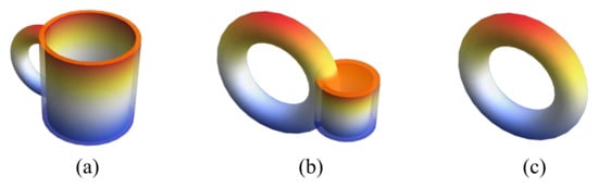
Figure 1.
Continuous deformation from (a) a mug, by way of (b) an intermediate phase, to (c) a torus.
2.1. Definition
A topology is defined as a set S and a collection of its subsets , such that:
- ;
- For any , ; k can be infinite;
- For any , , k is finite.
With these conditions, is said to give a ’topology’ to S [29]. For example, the power set formed by all subsets of ,
gives a topology to S, and the pair is a topological space. For short, we usually use S to refer to the topological space. Two topological spaces and are said to be homeomorphic to each other if there exists a map that is (i) one-to-one [Figure 2a], (ii) onto [Figure 2b], and (iii) for which both and are continuous [Figure 2c]. A topological space M is called a three-dimensional differentiable manifold if it has an open covering , such that for all , there exists a homeomorphism , and given , the composition map is differentiable [29]. Here, differentiable means having derivatives of all orders.
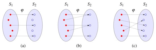
Figure 2.
Schematic illustration of a map between topological spaces and which is (a) one-to-one, but not onto, (b) onto, but not one-to-one, and (c) one-to-one and onto.
2.2. Topological Invariants
A property of a topological space that is invariant under homeomorphisms is called a topological invariant. There are various topological invariants, among which the most frequently used in condensed matter physics are the genus and the winding number. A topological phase transition occurs when there is a change in the topological invariant of a material. As an example, the non-trivial edge states protected by the time-reversal symmetry in a topological insulator is characterized by the number being equal to one [30,31]. In semimetals, different symmetries lead to different band crossings that are also topological invariants [32,33,34,35]. In superconductors, homotopy is applied to determining the winding number of the vortex created by breaking gauge symmetry [29]. Homotopy groups have been used for the topological classification of defects in ordered systems in terms of winding numbers [36,37]. Topology has also been applied to martensitic phase transformations, with the manifolds describing two end states having a point-group symmetry compatible with those of their corresponding phases [12].
Genus is defined as the maximum number of disjoint simple closed curves (’loops’) that can be drawn on a surface without a disconnection [38]. We cannot draw a loop on a sphere without cutting it into two parts [Figure 3a], but on a torus, a closed loop along the smaller circle will only cut the torus into a cylinder [Figure 3b]. Drawing a closed loop around a cylinder [Figure 3c] divides the cylinder into disconnected parts. On a surface that is compact, closed, and connected, the genus g is given by [39]:
where is the Euler characteristic of this surface, which can be obtained from the Gauss–Bonnet theorem [39]:
Here, K is the Gaussian curvature, and the integral is taken over the surface S. Intuitively, the Gauss–Bonnet theorem links a local property, K, to a global property, . This can be understood from the Gaussian curvature being an intrinsic property that can be obtained without referring to the embedding of this surface, and the Euler characteristic, which is invariant under continuous deformations and independent of the embedding [39].
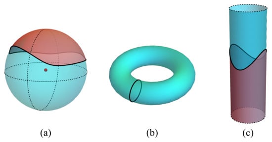
Figure 3.
(a) Drawing a loop on a sphere divides this sphere into two disconnected parts. The red and cyan regions in (a) are the disconnected parts of a sphere separated by this loop. (b) Drawing a loop on a torus does not yield a disconnection. (c) Drawing a loop around a cylinder divides the cylinder into disconnected parts, indicated by the red and cyan regions. All loops are indicated by bold curves.
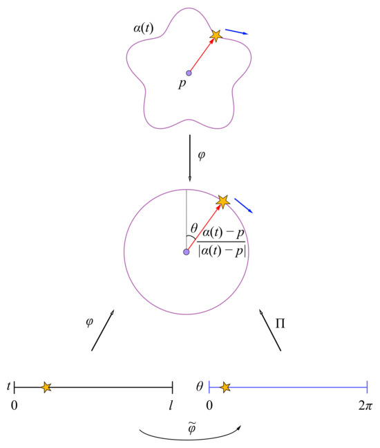
The winding number counts the number of times a continuous closed curve winds around a point. For topological materials, the winding number characterizes different phases that depends on the symmetry of the system. Mathematically, the winding number of a continuous closed curve around a point p is given by first taking a position map [29]:
then, by calculating the variation in angle in Figure 4, which gives the winding number:
where
and
2.3. Connections
Imagine that there is a boat moving along a curve in a plane. Then, the notion of ‘parallel’ means keeping the length and angle between a vector and a fixed direction invariant. Suppose that the curve is a straight line and we put a flag at the bow. As time passes, the flag maps out a trajectory, as shown in Figure 5a. If the curve is not a straight line, the boat will move up and down and the direction along which the flag points will also change [Figure 5b]. Hence, in Figure 5a, the flags at different times are parallel to each other, which means the flag is parallel-transported along the curve. However, in Figure 5b, flags at different times are not parallel to each other. If we want to maintain parallel transport, the flag should be allowed to point in directions that are not perpendicular to the line tangent to the curve and indicated by orange arrows, as shown in Figure 5c. Therefore, to describe the flag at a time in Figure 5c in the local coordinates moving with the boat, we need to know the tangent line and the direction normal to this line at that time, as well as the deviation of this flag from the normal direction caused by the curve.
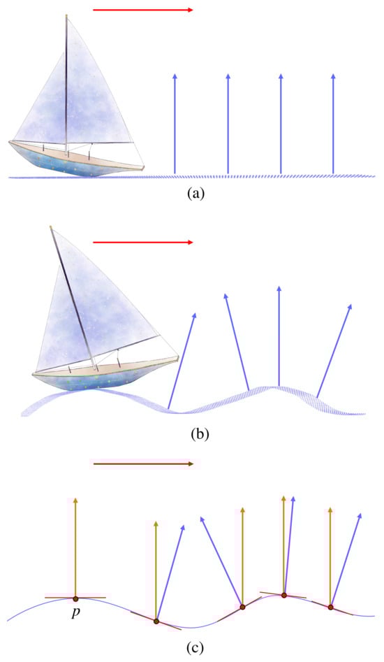
Figure 5.
(a) A ship moves along a straight line in a two-dimensional (2D) plane. Blue arrows show the direction of the flag when the ship is moving. All blue arrows in (a) are parallel to each other. (b) A ship moves along a curved line in 2D space. Due to the curvature, the blue arrows are not parallel to each other. (c) Orange arrows show vectors that are parallel to each other along the curve and blue arrows point in the normal direction to the curve at their corresponding points.
We now extend this argument to three-dimensional (3D) space. Suppose that we have a curve lying on a surface (Figure 6). The trajectory mapped out by the boat is the line , and the motion of the flag is defined by a vector field . At points , where , the corresponding vectors are . Then, the local coordinates have the basis , where and lie in the tangent plane at p, with being the unit normal vector at p to S:
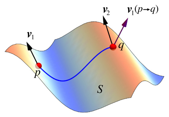
Figure 6.
A section of a surface . The trajectory mapped out by a boat travelling on this surface begins at and ends at . The variation is obtained by parallel-transporting from p to q.
A connection is defined as the map [29]
where are the th and th components of the vectors and , respectively, and is the coordinate basis. is called the connection coefficient [29]
If there is an observer on the boat moving from p to q, then, to this observer, the variation in the vector obtained by parallel-transporting from p to q is determined by the geometry of the surface. The ‘connection’ compares objects at different points, which thus can tell the variation in vectors after being parallel-transported along a curve that is determined by the surface geometry.
Although the main purpose of introducing parallel transport is for a discussion of connection and curvature, parallel transport has also been used in its own right to characterize the defects in liquid crystals [40,41]. The basic idea is that parallel transport of a vector tangent to a surface defines the topological charge of defects in a liquid crystal and how the defects interact and affect the properties of the liquid crystal, including its energy. Since the parallel transport of a vector around a closed loop yields the Gaussian curvature, which is an intrinsic measure of the curvature of a surface (see below), this method of characterizing defects in liquid crystals is referred to as an intrinsic method [41].
2.4. Curvature
Curvature is a property of the bending of a surface. The Gaussian curvature gives the change in the direction of a vector when it is parallel-transported around a loop. As shown in Figure 7, the vector points in another direction after being parallel-transported around a loop on a sphere. The mean curvature is also frequently used in applications. The mean curvature describes the embedding of a surface in a space that cannot easily be detected by a creature living in this surface. For instance, for a long time, people believed (and still do! [42]) that the earth is flat. The Riemannian curvature is an extension of the Gaussian curvature to spaces with a dimension higher than two. Similar to Gaussian curvature, Riemannian curvature tells how a vector is rotated after being parallel-transported around a small loop. The local shape near a point p on a smooth surface S is characterized by the principal curvatures and of the maximum and minimum bending near that point. The Gaussian curvature K can be expressed as the product of the principal curvatures and the mean curvature M can be expressed as the average of the principal curvatures:
Principal curvatures are defined as the maximum and minimum of the normal curvature , which is given by [39]
where is the unit normal p to S, is the unit normal of a curve at p, p is on , k is the curvature of at p, is the unit tangent vector at p to , and the corresponding tangent vector (Figure 8). The vector d shows how fast is pulled away from p along :
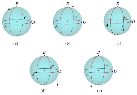
Figure 7.
The parallel transport of a vector along a curve following on a sphere. (a) The initial vector pointing upward, (b) , (c) , (d) , and (e), , where the vector points downward.
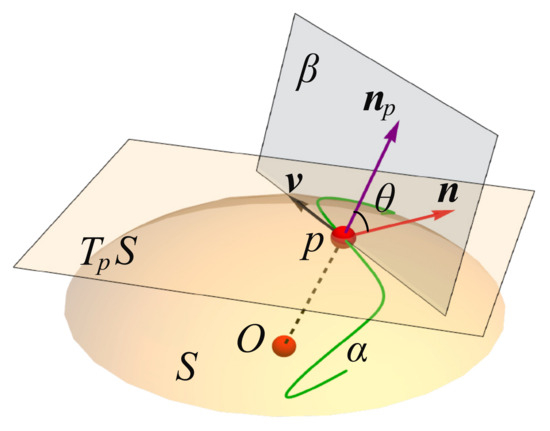
Figure 8.
A surface S and its tangent plane at p. Normal section at p along the direction tangent to the curve . The normal vector of at p equal to is along . is the normal vector at p to S. The angle between and is . is the radius of the curve at p.
2.5. Fiber Bundles
A fiber bundle generalizes the notion of a product space. A fiber bundle has two spaces: the base space B and the fiber F, such that at every point of B, there is a copy of the fiber. These fibers are connected continuously. In more fundamental mathematical terms, a fiber bundle is a geometrical object consisting of [29,43]:
- E: a differentiable manifold called the total space;
- B: a differentiable manifold called the base space;
- p: a surjection called the projection;
- F: a differentiable manifold called the fiber;
- G: a Lie group called the structure group that acts on F from the left. The special case of as a structure group is addressed in the following example.
For convenience, we often use E to denote the fiber bundle. A basic example of a fiber bundle is a cylinder surface, with the base space being a circle , and the fiber being a line segment . As illustrated in Figure 9, continuously attaching line segments to the central circle, a cylinder surface is ultimately formed, which has a structure group consisting solely of the identity. Such a cylinder surface is isomorphic to , the direct product of and I, and is called a trivial bundle. By opening this cylinder at an arbitrary site to form a strip, twisting it by 18, and gluing A to and B to (Figure 10), a Möbius strip is generated. An untwisted fiber (e.g., ) is operated on by the identity, while a twisted fiber (such as ) is operated on by a flip indicated by . Hence, the corresponding structure group is . The Möbius strip is a non-trivial bundle, as the introduction of a twist makes it non-isomorphic to . For a comprehensive mathematical explanation, refer to Refs. [29,43].
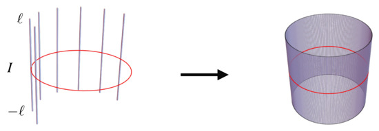
Figure 9.
Formation of a cylinder by attaching line segments at every point on a circle. The cylinder is isomorphic to the direct product of the circle and the line (the fiber) I: .
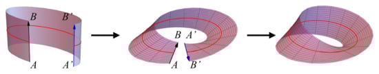
Figure 10.
Formation of a Möbius strip by twisting a rectangle strip. The Möbius strip is not isomorphic to the direct product of the circle and the line.
In crystalline materials, the topology of the electron’s energy band structure is determined by the structure of the associated Bloch bundle, where the fiber is the effective Hilbert space at each quasi-momentum , and the base manifold is a d-dimensional torus (BZ), where d is the dimension of the crystal lattice. In insulators (trivial or non-trivial), an energy gap exists in the bulk of the crystal and the band structures on either side of the gap form a Bloch bundle of their own energy, for the conduction band and for the valence band. If the band structure arises from a single Hamiltonian, then the energy bands on either side of the gap are coupled by the Hamiltonian. The fiber at of the coupled Bloch bundle is the direct sum of the fiber of the conduction band and the valence band at . Topological invariants such as the Chern number and the invariant are obtained by integrating their corresponding two-forms (Section 4 and Section 5) over the whole Bloch bundle so that they can reveal the global geometry of this manifold.
Given a set of topological invariants of (the same for and ), their value will remain the same under symmetry-compliant perturbations to the Hamiltonian without closing the band gap. Fiber bundles , , and of a gapped system are topologically trivial if the valence and conduction bands are isolated from other bands, allowing for the identification of a globally smooth gauge for the Bloch function. This condition permits the existence of exponentially localized Wannier functions. However, if the gap closes and reopens, that results in an obstruction to finding a smooth gauge on and , so and are topologically non-trivial. The Berry connection, introduced later in Section 4, serves as an example of a gauge to choose. This obstruction arises either from a band inversion (‘twist’), or a change in the configuration of or , or both. The topological inequivalence of a cylinder and a Möbius strip caused by a twist helps to understand the variation in the topology of and caused by a ‘twist’ in the bundles. Topological insulators exhibit a dual behavior: they function as electronic insulators in the bulk while possessing conducting states on their surfaces. This can be addressed as follows. At the boundary between any two phases of distinct topological orders, the boundary conditions cannot maintain a continuous interpolation of the band structure across the interface, leading to surface/interface state in the gap. Further detail can be found in Refs. [44,45].
3. Triply Periodic Minimal Surfaces
A surface whose mean curvature M vanishes everywhere is called a minimal surface. The name ‘minimal’ comes from the minimization of the surface free energy. According to the Young–Laplace equation [46], the pressure difference between two sides of a surface is proportional to the mean curvature. Given that the surface free energy is proportional to the surface area that is minimized when , we see that when , the surface free energy will be minimized. One example of a minimal surface is the catenoid. If a minimal surface repeats along three independent directions, then this surface is called a triply periodic minimal surface (TPMS). The concept of a TPMS was first proposed by Schwarz [47]. Figure 11 shows examples of TPMSs.
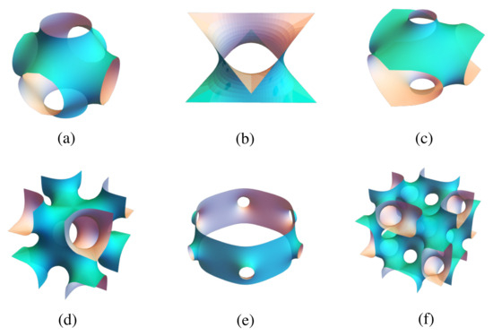
Figure 11.
Sections of TPMSs: (a) a P surface. (b) a D surface, (c) an H surface, (d) an I-WP surface, (e) an -T surface, and (f) an F-RD surface.
Our application to martensitic transformations regards a TPMS as a charge density template for crystal structures and their transitions. But TPMSs have also been found to exist in natural systems, such as the sea urchin plate [48] and the diamond-based structure in beetles scales [49]. Thus, TPMSs can be designed as physical structures based on natural structures, where the high surface-to-volume and strength-to weight ratios, tunable mechanical properties, and other characteristics are explored for many applications. Improvements in additive manufacturing, which is also known as three-dimensional printing and is the process of creating an object one layer at a time, have enabled TPMSs to be fabricated for specific applications [50]. Examples include biomimetic scaffolds [51], architecture and interior design [52], thermo-mechanical applications [53], thermal management [54], and carbon allotropes [55].
3.1. Presentations of Minimal Surfaces
Triple periodicity requires the TPMS to have a genus of at least three [56], as we now show. Consider a cube [Figure 12a]. This surface can be made triply periodic by constructing periodic boundary conditions in the three coordinate directions. Being triply periodic means surfaces , , and are equivalent to , , and , respectively. Hence, we can attach to [Figure 12b], yielding a torus, which is the Cartesian product of two circles. Repeating this process to the rest of the surfaces [Figure 12d], produces a three-torus, the Cartesian product of three circles. The three-torus is homeomorphic to the surface in Figure 12e. According to the Gauss–Bonnet theorem, a three-torus has a genus of three. Hence, a figure that is triply periodic must have at least a genus of three to ensure the periodicity.
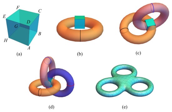
Figure 12.
The effect of imposing periodic boundary conditions in successively higher dimensions. (a) A cube. (b) Figure formed by attaching surfaces to in (a). (c) Figure formed by attaching surfaces to in (b). (d) Figure formed by attaching surfaces to in (c). (e) Three-torus that is equivalent to (d).
The Weierstrass representation is usually applied to describe a TPMS [56,57,58]. In a Cartesian coordinate system , the Weierstrass representation is given by:
where in , the integral is taken in , gives a doubly periodic function defined in (a Riemannian sphere), and dh is the height differential. The reason why a Weierstrass representation is presented in such a form comes from projecting the TPMS onto with the periodicity being preserved. That is to say, because deriving an expression for a TPMS in the 3D space is complicated, one can project this surface along one direction exhibiting a periodicity onto a 2D plane (), derive a doubly periodic expression of this image, then project this expression back to a 3D space along . The Weierstrass expression is a projection from to . A TPMS has space-group symmetries. The translational subgroup describes its triple periodicity. There is also an associated crystallographic point group. When the space group is symmorphic, the point group is also a subgroup of the space group. Symmetry groups of the TPMS given in Figure 11 are compiled in Table 1.

Table 1.
The space group, the point groups, and the genus of the TPMS in Figure 11 [59].
3.2. Martensitic Phase Transformations and the Shape-Memory Effect
Hyde and Andersson [10,11,12,13] first attempted to use a continuous deformation of a TPMS to explain the – martensitic phase transformation in iron. A martensitic phase transformation is a diffusionless phase transformation in which atomic displacements are smaller than an atomic spacing and is realized by shears of atomic planes. A shear is a relative movement of an atomic layer with respect to another in a direction parallel to that layer [Figure 13a]. The – iron phase transformation is one example of the martensitic phase transformation. After a rapid quench, the iron transforms to its phase. In a martensitic phase transformation, the high-temperature phase is called ‘austenite’ and the low temperature phase is called ‘martensite’, after the German metallurgist Adolf Martens, for his contribution in studying the microstructures of steels [60,61]. In addition to iron, zirconium [62], CuAl [63], CuSn [64], and perovskites such as BaTi [65] are also martensites discovered later in the 20th century. If a material deformed in its martensite phase can recover to its original shape after heating to its austenite phase [Figure 13b], this material is called a ‘shape-memory material’. NiTi [66] is the best-known shape-memory material and has been used, for example, to fabricate self-locking couplings in aircraft [66].
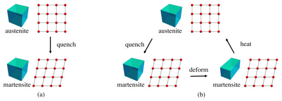
Figure 13.
(a) Schematic illustration of a (a) martensitic transformation, and (b) the shape-memory effect based on a martensitic transformation. In (a), the material is first cooled from a high-symmetry parent phase (austenite) to a lower symmetry phase (martensite). In (b), after cooling to the martensite phase, a temporary shape of the material can be produced by deformation in that phase. The austenitic phase is reached upon heating the sample above the phase transition temperature with a recovery of the original external shape for deformations of 5–10%.
Various methods have been proposed to study the martensitic phase transformation and the shape-memory effect, which can be categorized into two classes: (i) computational and (ii) theoretical. Computational methods include those based on the density functional theory (DFT) and/or molecular dynamics that either calculate the energy barrier along the phase transformation [67,68,69,70,71,72,73,74,75], or find the critical temperature by examining the softening of phonon modes [76,77,78,79,80]. Shape-memory alloys, such as NiTi [67,68,69] and Ti-Ta [73], have a vanishing energy barrier along some paths. Ordinary martensite materials, such as Zr [74] and Fe [70,71], do not have a barrierless transformation path.
Martensitic phase transformations with two end phases related by a group–subgroup relation, in either their space group or point group, can be described in the framework of Landau’s theory of second-order phase transformations [81,82,83,84,85]. The reason why a group–subgroup relation is required here is the variation in charge density, chosen to be the order parameter. Because the charge density of a crystal (as an observable) is invariant under the symmetry group G of this crystal, the charge density can be written using basis vectors of a vector space that is invariant under G. If there is a group–subgroup relation, the vector space V of the lower symmetry phase will be an invariant subspace of the vector space under the operation of the subgroup. Hence, the charge density can always be expressed using basis vectors of . If there is no such group–subgroup relation, then there will be vectors that do not belong to , which means there will be no continuous change in the charge density. However, Landau’s theory requires a continuous change in the order parameter. For materials with no group–subgroup relation, Tolédano and Dimitriev [82] adapted Landau’s theory and proposed a reconstructive theory. Hyde and Andersson [10,11,12,13] also employed a continuous deformation between TPMSs to explain the martensitic phase transformation from body-centered cubic (BCC) iron to face-centered cubic (FCC) iron.
3.3. Triply Periodic Minimal Surfaces and Density Functional Theory
Schnering and Nesper [86,87,88] found that the zero equipotential surfaces (ZEPs) in an electrostatic field in crystals resembled TPMSs. In most biological and chemical applications mathematical, ZEPs are usually adopted because the corresponding TPMSs are given in terms of algebraic expressions of trigonometric functions. An altogether different approach is described in Ref. [89], where the electronic structure is obtained with the DFT, which includes exchange and correlation between electrons. A semi-classical approach based on the Boltzmann equation shows that surfaces of zero charge density correspond to the TPMS for the structure of the given material.
Figure 14 shows a section of a TPMS of a constant charge density as this constant approaches zero. The example shown is for a section that corresponds to B2 NiTi, which has a simple cubic structure. As the surface of constant charge density approaches zero, the convergence to the P surface is evident. For the largest deviation from zero charge density in Figure 14a, as measured by the root-mean-square (RMS) deviation from the P surface [89], the basic shape of the P surface has formed, but there are differences in detail between the exact surface [Figure 14d]. As the constant charge density decreases, the fine structure of the P surface is reproduced by the charge density surface until, for the smallest value in Figure 14c, the RMS difference from the P surface is a minimum. While the resemblance between this section of the P surface and the Fermi surface of a simple cubic lattice is striking ([90], p. 231), and this Fermi surface in the periodic zone scheme is similar to the P TPMS, this must be regarded simply as a coincidence. The Fermi surfaces of other materials, such as Cu ([90], p. 235), bear no resemblance to the TPMS of Cu [89].
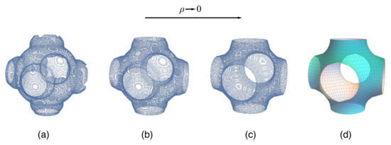
Figure 14.
The approach of the constant charge density surfaces to the P TPMS corresponding to B2 NiTi as this constant approaches zero. The constant in (a) is greater than that in (b), so, although the surface shares some similarities with the TPMS, there are still discernible differences. The surface of approximately zero charge density in (c) is closest to the TPMS in (d).
The TPMS obtained from DFT calculations satisfy the following: (i) the TPMS is compatible with the Bravais lattice of the crystal, (ii) the periodicity of the TPMS conforms to the periodicity of the crystal given by its corresponding basis vectors, and (iii) the TPMS is either in the same space group as the crystal or can exhibit the space group of the crystal by modifying the repetition unit of the TPMS [89]. Na, Al, Cu, and Zr, which have the BCC lattice (space group are described by the I-WP surface; Al and Cu in the FCC lattice (space group ) are described by the F-RD surface; and Na and Zr in the hexagonal close-packed (HCP) lattice (space group ) are described by the -T surface. By referring to Table 1, we see that the end phases of a martensitic phase transformation are described by TPMSs of the same genus [91]. TPMSs have also been applied in studying the shape-memory effect, where the TPMSs of shape-memory alloys have a transformation path that can be described by a continuous deformation between TPMSs within the space of TPMSs [91].
4. Dynamical Phase and Geometric Phase
Consider the adiabatic evolution of an eigenstate of a Hamiltonian when the external parameters of the Hamiltonian change slowly over a loop in parameter space. In the absence of degeneracy, the eigenstate returns to itself when completing the loop, but there is a phase difference equal to the time integral of the energy plus an extra term, which is now known as the Berry phase [92]. The Berry phase has three important properties: (i) gauge invariance, meaning the freedom of multiplying the wave function by an overall phase factor which can depend on the parameters; the Berry phase is unchanged up to an integer multiple of , provided the eigenfunction is single-valued over the loop; (ii) geometrical, in that the Berry phase can be written as a loop integral of the Berry connection in parameter space that does not depend on the rate of change around the loop; and (iii) close analogies to differential geometry [93], so that the integral of the Berry curvature over closed surfaces is topological and quantized as integers known as Chern numbers in even dimensional spaces.
In this section, we derive the Berry phase from the adiabatic evolution of the Hamiltonian around a closed loop in parameter space; we then consider the Berry connection and the Berry curvature before considering the application of these concepts to a two-level system. We conclude with a more general description of topological materials. Among the many books and review articles that have been written about the Berry phase and topological materials, those we found particularly useful are Refs. [29,92,94,95,96].
4.1. Adiabatic Evolution
Suppose we have a Hamiltonian that depends on a set of parameters written as . The Hamiltonian, the energy, and the wave function depend on the time through their dependence on the time-dependent parameters. Consider an adiabatic process during which the parameters change slowly over time. The wave function is a solution of the time-dependent Schrödinger equation:
where we use the abbreviated notation and , that is, various quantities acquire a t-dependence through their dependence on . The complete set of eigenstates of satisfy the eigenvalue equation
According to the adiabatic theorem [97], there is a phase difference between and , part of which turns out to be the Berry phase:
Substituting the right-hand side of this equation into the time-dependent Schrödinger Equation (15),
and projecting onto yield an equation of motion for the phase:
The first term on the right-hand side of this equation can be written as
Thus, integrating (19) over a path from to t yields
The first integral on the right-hand side of this equation is known as the Berry phase, which depends on the path but not on the time. The second integral is the dynamical phase, which depends on both the path and the time. An overall phase factor has no observable effects. However, when there is more than one subsystem, the Berry phase accounts for a phase difference depending on the path, which does produce observable effects.
4.2. Connection and Curvature: Analogy with Electromagnetism
Suppose that we multiply the states of the system by an overall phase , where is a smooth, real-valued function. The integrand in (21) becomes
which is not gauge-invariant and is analogous to the vector potential of electromagnetic theory. However, substitution into (21) and using Stoke’s theorem yield
which shows that the Berry phase is gauge-invariant when taken around a closed path. Thus, the Berry phase is well defined for closed paths in a parameter space. To pursue the electromagnetic analogy, we use the notation
which is the Berry connection. As (22) shows, because the Berry connection is not gauge-invariant, it cannot be observed.
In a three-dimensional parameter space, Stokes’ theorem can be used to obtain the Berry phase by evaluating the integral of the Berry connection over a closed path :
where is the Berry curvature associated with the Berry connection. If we think of as a vector potential, then is the magnetic field. By multiplying the wave functions by an overall phase , we obtain from (22)
because the curl of a gradient vanishes. Hence, the curvature is gauge-invariant. The Berry curvature is a two-form, that is, a tensor defined on a manifold, given by (Einstein’s summation convention is used here):
where run over the dimension of the system and and belong to an orthonormal basis. We can also create -forms by taking the wedge product of by m times. More details can be found in Ref. [29].
The relation between the differential geometry, connection, and curvature, as discussed in Section 2.3, and those defined by the Berry phase is summarized in Table 2. This table shows that topological phenomena are robust because, under a continuous deformation of a physical systems, many physical observables should also change in a continuous fashion. Topological invariants are labeled by integers, so integer changes are discontinuous. This is analogous to the winding number, which is a topological invariant, meaning that it cannot be changed without crossing the origin, viz., closing the band gap.
Table 2.
The relationship between differential geometry and topology and the corresponding quantities used to characterize topological insulators.
4.3. Two-Level System
As an example of how the Berry phase is calculated, consider the Hamiltonian of a generic two-level system:
where is the vector of parameters, and is the vector of Pauli matrices:
In addition to having the form of the Hamiltonian for the two-band model of graphene, this basic Hamiltonian appears in the description of several types of physical systems, including linearly conjugated diatomic molecules, one-dimensional ferroelectrics, and certain types of quasiparticles. By parametrizing in terms of a polar angle and azimuthal angle ,
where , , and , and the Hamiltonian (28) becomes
This Hamiltonian can be represented as a Bloch sphere, as shown in Figure 15. The eigenstates of H corresponding to the eigenvalues are written as:
These wave functions may be multiplied by an arbitrary constant phase with no effect on their normalization and orthogonality.
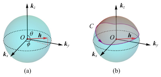
Figure 15.
The Bloch sphere corresponding to the two-level Hamiltonian in (31). The eigenvalue depends on the length of and the eigenstates depend on the direction of that is given by and , as shown in (a). Integrating the Berry connection along the curve C gives the Berry phase, as shown in (b).
Consider the wave function corresponding to the lower energy level. The components of the Berry connection are
from which we obtain the Berry curvature as
By writing this Hamiltonian in Cartesian coordinates, , we obtain,
which is the field generated by a monopole at the origin , where the two energy levels become degenerate. Therefore, degeneracy points act as sources and sinks of the Berry curvature flux. By integrating the Berry curvature over a sphere containing the monopole, we find
In general, the integral of the Berry curvature (two-form) over the closed 2D manifold is quantized in units of and corresponds to the net number of monopoles enclosed by the manifold. This defines the ‘first Chern number’. To calculate the integral of a k-form over a manifold of dimension d, it is necessary to have ; otherwise, the integral evaluates to zero. It follows that if , there is a loss of information in the remaining dimensions when integrating the k-form over the entire manifold. For instance, it is not possible to integrate an infinitesimal surface patch over the entirety of the three-dimensional space because of the uncertainty in its way of stacking along the third dimension. Consequently, the Chern number is exclusively definable in even-dimensional spaces. In odd-dimensional systems, one may refer to alternative topological invariants, such as the invariant [98], or the adapted Chern number, including the Chern vector [99] and the Chern number of higher classes.
The Berry phase, as defined in (21) for non-degenerate state (one band), can only be computed for isolated bands. It can be computed only if the Hamiltonian yields no degenerate states. For a Hamiltonian with many bands , where n is again a band index, this means that we can compute the single band’s Berry phase only for a system of isolated bands that do not touch one another. If there is touching between any bands, the single band’s Berry phase is undefined. In terms of our analogy between the Berry phase and electromagnetism, we cannot compute the electric or magnetic flux through a surface if there are electric or magnetic charges located on the surface because the electric or magnetic fields are not defined at the points where their sources are. This analogy suggests that the sources for the Berry flux in momentum space are points where two bands touch, such as the Dirac points at the K and points of the Brillouin zone in graphene.
When degeneracy occurs in energy eigenstates along the closed loop (connected multi-bands), further development based on time-dependent perturbation theory (Section 4.5 and Sections 6.6 and 6.7 of Ref. [100]) is required. The Berry connection is path-dependent (non-Abelian) and the adiabatic evolution of the eigenstates are described by the Wilson loop . A generalized Berry phase is defined as in terms of a Wilson loop. A comparison with electromagnetism is then not possible as the gauge field is non-abelian.
4.4. The Bulk–Boundary Correspondence
A key signature of topological insulators is the bulk–boundary correspondence. This correspondence states that the multiplicity of conducting edge states on the boundary of a topological insulator are characterized by the topological invariants of the bulk energy bands. Edge states exhibit remarkable properties that are distinct from bulk states, including robustness against certain types of disorder and impurities. This robustness is said to endow edge states with symmetry protection. The bulk–boundary correspondence has been verified in experiments and numerical simulations. For example, the bulk Hall and edge conductance values of a topological insulator are quantized precisely, even in the presence of defects and disorder.
There is no general theory for the bulk–boundary correspondence. Much of the difficulty originates from the fact that edge states and the topological invariants of the materials require different types of analysis. The edge states require the presence of boundaries. However, topological invariants are calculated from bulk energy bands, whose calculation is based on the translational symmetry of the lattice. As in introductory solid-state physics, this means either that the system is infinite or, if finite, periodic boundary conditions are applied at the edges. As a result, topological systems have been treated on a case-by-case basis, with the quantum Hall effect, the Su–Schrieffer–Heeger, Kane–Mele, and Qi–Wu–Zhang models being among models where the bulk–boundary correspondence can be addressed explicitly [30,31,101].
Despite there being no general theory of the bulk–boundary correspondence, there are statements one can make about edge states in particular cases:
- Edge states occur at the interfaces between materials with different topological invariants (including the vacuum) with different topological invariants, such as Chern numbers and indices.
- The number of edge states is equal to the difference in topological invariants across an interface.
- Edge states take various forms, depending on the underlying topological phase and symmetries of the system.
- Types of edge states include chiral edge states (quantum Hall effect) [102,103,104], helical edge states (quantum spin Hall insulators) [30,31,105,106], and Majorana edge states (certain one-dimensional superconductors) [107,108].
4.5. Degenerate Energy Levels
The analysis in Section 4.1 leading to Berry phase can be extended to degenerate energy levels [109]. We again begin with a Hamiltonian that depends on a set of parameters written as . The evolution of this Hamiltonian in parameter space is adiabatic, and the Hamiltonian is assumed to be the same for all times, that is, there are no level crossings. The energy level is n-fold degenerate, and we suppose that form a basis for the eigenspace of the n-fold degenerate states. In keeping with Section 4.1, various quantities acquire their time-dependence through . Therefore, to simplify the notation, we write and , for .
Since the evolution is adiabatic, the eigenvectors of the Hamiltonian must span the same space as the basis states along the trajectory:
where are the entries of an matrix. In fact, to maintain orthonormality of the eigenfunctions along the trajectory, this matrix must be unitary. Substituting into the time-dependent Schrödinger Equation (15),
and taking the inner product with yield:
By substituting (38) and its Hermitian conjugate into the right-hand side of this equation, we obtain:
Using the orthogonality of the and the fact that
are the entries of an anti-Hermitian matrix, (41) can be written as
These are the th elements of the following matrix equation:
where is the unit matrix. By operating from the left by and from the right by , we obtain [109]:
This equation can be solved by first writing it in the form:
We now consider an infinitesimal time :
Any path can be divided into incremental steps and then summed, leading to [109]:
The first term on the right-hand side is the dynamical phase. The second term is the extension of the Berry phase to degenerate states. This is known as the Wilson loop , and the Berry phase in bands with degeneracy is defined as . The path ordering, indicated by , is necessary because matrices at different times do not commute. Thus, the gauge potential is non-Abelian. Note that there is no extension of Stokes’ theorem for this case, so the phase change cannot be related to a gauge-invariant quantity, such as the solid angle subtended by the circuit in parameter space [94].
5. Topology of Energy Bands in Crystalline Solids
The electronic energy dispersion surfaces of a crystalline solid are embedded in the triply periodic manifold of the Brillouin zone (BZ) in the wave vector space. Within the topological band theory [110], the one-electron eigenstates span the tangent space of the Bloch bundles at a given wave vector defined in the base manifold of the BZ. The wave vector serves as a quantum number and a label of the irreducible representations of the space group . The eigenstates are components of irreducible representations or irreducible co-representations (of the time-reversal invariant system) of the space group labeled by . Due to Bloch’s theorem, the BZ is triply periodic in the wave vector space. In one, two, and three dimensions, the BZ is a circle, a two-torus, and a three-torus, respectively, forming a closed, but not simply connected, manifold (Figure 12). This is illustrated in Figure 16 for graphene with the sub-periodic layer group 80, with defined as the representation domain (RD). While the plane group is frequently used for two-dimensional systems, the use of the sub-periodic layer group is necessary when electron spin is considered. The spin is only meaningful when the rotations are elements of a subgroup of SO(3), which is non-Abelian and whose double cover is SU(2). The rotational parts of plane groups are always elements of the subgroup of the Abelian group SO(2).
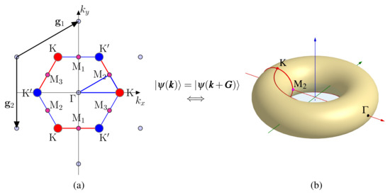
Figure 16.
Brillouin zone of graphene as a triply periodic manifold. (a) Normal reduced zone view, with defined as the representation domain, indicated by the triangular region outlined by the blue line. (b) A torus, with two equivalent uncontractible closed paths indicated by red curves.
One of the key impacts of topology is the existence of the bulk–boundary correspondence in topologically non-trivial phases, which leads to edge states in their energy gap [9] (Section 4.4). The classification of these dispersion surfaces of connected bands is investigated by the study of parallel transport [92,111], such as the Berry phase (Section 4) or invariants. For multi-band system with degeneracies, they are based on the Wilson loop [100,109], which describes the adiabatic evolution of energy eigenstates in connected bands in wave vector space. For N connected bands, the non-Abelian Berry connection and the Wilson loop with base point and uncontractible path are defined as:
Here, m and n are the indices of the connected bands, each of the eigenstates is a component of the bases of the irreducible representations of the space group, and the integration path of the Berry connection is taken along a closed uncontractible path on the BZ manifold. Any symmetry operation would permute the eigenstates among those labeled by the star of and the integration path among a set of equivalent paths. The generalized Berry phase is then defined in terms of the Wilson loop:
The eigenvalues of are of the form and are gauge-invariant. The element of the Wilson loop and are generally gauge-dependent, but is gauge-invariant, with defined modulo .
For systems with time-reversal symmetry, the Wilson matrix describes the evolution of eigenstates at and . These energy eigenstates are components of the same irreducible co-representation of the space group [112] labeled by . Thus, the Berry phase is defined for two paths and in such time-reversal symmetric systems, where the Berry connection is in block diagonal form, with each block corresponding to one of the two paths. Acting on one block with the time-reversal operator yields the other block. As a whole, the band indices run over the components of all relevant co-representations of the space group at and . For time-reversal symmetric systems, an alternative Berry phase is defined:
The alternate Berry phase yields the invariant [113] when the extended path encloses half of the BZ in two-dimensional systems. In both cases, the closed-path integral of the Berry connection with respect to the energy eigenstates is involved.
These Berry phases, based on the Wilson loop, are the holonomy of the Berry connection and generally defined in all dimensions. In 2D, it is equivalent to the first Chern number, when the path is extended to enclose the whole BZ. However, its gauge dependence means that special techniques are required to extract the Chern number from Berry phase. In a time-reversal symmetric 2D system, is equivalent to the invariant when the closed path covers half of the BZ. Time-reversal symmetry forbids the first Chern number in 2D but allows the invariant. A zero (and zero in time-reversal symmetric systems) indicates that the connected bands are topologically trivial. It is hypothesized that there is an absence of a bulk–boundary correspondence (Section 4.4) in such connected bands. The definition of here makes use of the full eigenstates, instead of the frequently used cell-periodic function . The role of symmetry is made more explicit in the following sections. Direct evaluations of these topological invariants are particularly difficult because of the non-Abelian SU(N) gauge group [109] encountered at degeneracies present in the connected bands (Section 4.5). For these reasons, the primary approach in the classification of topological phases of dispersion surfaces are based on a symmetry analysis.
6. Topological Quantum Chemistry and Band Representations
Topological quantum chemistry (TQC) aims to classify the topological phases of electronic dispersion surfaces of connected bands based on band theory and symmetry [114,115,116]. It also enables the discovery of topological phases in new materials. A primary hypothesis is that any connected bands are topologically non-trivial if they cannot be continued to the atomic limit without breaking symmetry or closing the gap (Definition 1 in Ref. [114]). This is equivalent to defining connected bands with an atomic limit as topologically trivial, since they are separated from those defined in the hypothesis by a topological phase transformation. In other words, connected bands with a full-real-space Wannier function [117,118] description are topologically trivial. When Wannier functions centered on all atomic positions (crystallographic orbits of Wyckoff positions) are considered, they form a representation of the space group in real space. Thus, the problem is reduced to finding the transformation properties of these representations in wave vector space and identifying connected bands with the same transformation properties. Connected bands with different transformation properties, including band connectivity, are then considered topologically non-trivial.
The Bloch sum constructed from these Wannier functions is used in the tight-binding (TB) model of Slater and Koster [119]. The Fourier transform of these Wannier functions with respect to the coordinates of their centers (the crystallographic orbits of Wyckoff positions) were formally defined as the band representation (BR) by Zak [120]. The Zak and TB Bloch sums are
Here, are Wannier functions centered on the crystallographic orbits of Wyckoff positions generated by the lattice vector and Wyckoff position within the primitive cells. The Wannier functions transform according to the irreducible representation of the site symmetry group () of the associated Wyckoff positions. The two definitions differ by a -dependent gauge term. As the Berry phase along any closed path is gauge-invariant (Section 4), a symmetry analysis based on either definition should be the same.
Equation (52) has the advantage of containing no explicit -dependence in the rotational part of its transformation properties. This simplifies the symmetry analysis on the transformation of with respect to the band representation bases or its linear combinations on the index. A band representation is defined as an elementary band representation (EBR) if the associated Wyckoff position is ‘maximal’ (it is not maximal if its site symmetry group is a subgroup of another site symmetry group under the same space group). It is considered a ‘minimal’ basis (building block) of TQC [114,121,122]. A set of EBR bases together form the composite band representation (CBR). An EBR induced from Wannier functions incorporating the spin degree of freedom is known as a physical EBR (PEBR) [114].
The transformation properties of fully connected EBRs are well established [121,123]. It has long been recognized that band connectivity [124] plays an important role in the topological order of the connected bands. The energy eigenstates under band theory are naturally the component of irreducible representations of the space group labeled by in the representation domain (Figure 16). Under the TB model, the CBR bases describing a set of physical bands are also decomposable into direct sums of irreducible representations of at . There is a one-to-one correspondence between the set of irreducible representations of eigenstates at described by the EBR/CBR bases and the decomposition of the bases themselves. There is also a one-to-one correspondence between the connected bands and how the nodes/terminals, represented by irreducible representations from the decomposition of EBR/CBR bases at high-symmetry points (HSPs), are connected. The symmetry of eigenstates at points are well defined by the decomposition of EBR/CBR bases. The connection between eigenstates at any HSP in the BZ and its immediate lower symmetry neighbors are governed by the compatibility relations [125]. However, such relations do not determine absolutely the connection between HSPs separated by lower-symmetry neighbors. Graph theory [126] and combinatorial techniques [116] were developed to establish configurations of band connectivity for the set of irreducible representations at HSPs obtained from the decomposition of EBR/CBR bases. Such band connectivities obey compatibility relations, but there was no methodology to identify band connectivities compatible with EBR/CBR bases and those with an atomic limit until recently (see Ref. [127] and Section 7).
Given a physical band structure, a set of connected bands is identified by a vector whose components are the multiplicities of all irreducible representations at all HSPs in the BZ [122,128]. The similarly defined vector can also be established for all EBRs under the same space group. Based on the hypothesis of TQC, connected bands, whose cannot be expressed as linear combinations of with integer coefficients, are considered topologically non-trivial. In other words, they cannot be represented by the EBR/CBR bases, cannot be continued to the atomic limit, and, therefore, are topologically non-trivial. This is the basis of the symmetry indicator method.
Whilst TQC has been used successfully in many publications, there are some unresolved issues. First, it is not clear if the hypothesis of TQC is equivalent to the classification based on the topological invariants and . There is an absence of symmetry-based selection rules for topological invariants linking the hypothesis to the invariant-based classification. It is also known that the band represented by the EBR induced from Wannier functions of the trivial irreducible representation centered on Wyckoff position 4b under space group F222 () has a non-zero Berry phase [129,130]. This appears to be a contradiction to the hypothesis but considered as a ‘Berry obstructed atomic limit’. It is also known that the EBR induced from Wannier functions centered on a Wyckoff position with multiplicity can represent gapped systems [131]. There are situations where such EBRs are known as decomposable [132]. It is assumed that the topological order of bands on either side of the gap are non-trivial [114], or at least one side is non-trivial [122]. Indeed, there is no clear criteria on the identification of the existence of the atomic limit and its requirement on the EBR. There are many exceptions to the rules and it is not clear if the symmetry indicator method identifies all topological phases. We attempt to address these questions using a symmetry analysis based on projection operators and the general matrix element theorem [133,134].
7. Band Representations, Connectivity, and Irreducibility
Band representations are induced from Wannier functions which transform according to an irreducible representation of the site symmetry group . It is defined for all in the BZ. From the transformation properties of the EBR defined in (52), the subduced representation of the little group of () is [127]:
Naturally, the general element of the space group is subject to the restrictions and . The relevant symbols are defined as follows. represents the representation matrices of the group shown in its superscript. The subscripts to indicate how it is obtained from the induction/subduction process. An up-arrow (↑) indicates an induction from the representation of the group to its left. A down-arrow (↓) indicates a subduction from the representation of the group to its left. Thus, Equation (53) shows the representation matrices of the little group of subduced from the BR of space group , which is induced from the irreducible representation of the site symmetry group . The ’s are defined as the chosen coset representatives in the left coset decomposition of the isogonal point group F in terms of , corresponding to the equivalent Wyckoff position , i.e., for some lattice translation . The matrix is defined in terms of two other matrices:
where the matrix defines how the equivalent Wyckoff positions are permuted under the action of group element:
and , where is the irreducible representation of . When , there exists . The last symbol is zero unless is an HSP on the surface of the BZ. In that case, it can be a reciprocal lattice vector.
The irreducible representations of the little group of () can be defined as those induced from irreducible representation p of the little co-group of ():
where again, a general element of the space group is subject to the restrictions and . From these, the decomposition of the EBR at in the BZ can be performed. This allows the normal analysis based on compatibility relations, generating configurations of band connectivity. Consider the EBR induced from the -orbital centered on Wyckoff position 2b of a honeycomb lattice. Compatibility relations yield two possible connections between different nodes in the BZ, as shown in Figure 17. However, only one of the two correspond to the EBR, and the compatibility relation cannot resolve this.
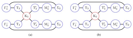
Figure 17.
(a,b) Connected graphs related to the band structure, described by the spinless EBR induced from the -orbital centered on Wyckoff position 2b of a honeycomb lattice, based on compatibility relations and graph theory. The degeneracy that existed at K ensures the system is in the semimetal phase for the half-filling of the band. Only configuration (a) corresponds to an atomic limit, when it is determined from projection operators.
7.1. Projection Operators and Band Connectivity
Beyond compatibility relations, one can define projection operators at any point in the Brillouin zone to obtain the linear combination of components of the EBR/CBR for a given node (irreducible representations of the space group labeled by p of the little co-group of ()). With the subduced representation of from EBR matrices in Equation (53) and the irreducible representation of in Equation (56), such projection operators are defined as
Here, is in the BZ, p is the label of the irreducible representation of , i and j are the indices of the irreducible representation p, and are the indices of the irreducible representation of the site symmetry group () of the EBR, and is the dimension of irreducible representation p. When the summation of the translation invariant subgroup is performed, the projection operator is given by
These projection operators have the usual properties.
where is contained in the vector space described by the EBR, and are the normalized bases of irreducible representation p. In particular, Equation (59a) preserves the sign in the sense that yields . Equation (59b) yields the correct signs between component j and component i of the multi-dimensional irreducible representation p.
Such projection operators, which do not involve any interaction described by the Hamiltonian, can be used to identify configurations of band connectivity permitted by the EBR/CBR bases independently of any interaction. Physical dispersion surfaces, which are equivalent by homotopy to such configurations of band connectivity, can be continued to the ‘atomic limit’ without breaking symmetry. Consider two nodes in the connected bands at and , which are separated in the BZ with irreducible representations p and q, respectively. Successive application of projection operators yields
where is some state described by the EBR bases. Then, the vector evolves continuously from into some state at . Since , a link between node/termina an must be possible. In fact, there are three possibilities:
which correspond to Equation (61a), for an exclusive link between the two nodes/terminals called a simple link; Equation (61b), for a possible link between the two nodes/terminals called a complex link; and Equation (61c), where no link can exist between the two nodes/terminals at the next nearest neighbors in bands described by the EBR bases. The complex link implies a possible link may exist between multiple terminals where
and so on, are also true. Consider the EBR induced from the -orbital centered on Wyckoff position 2b of the honeycomb lattice. The links that exist between nodes/terminals are shown in Figure 18. Links associated with nodes at K are all complex.
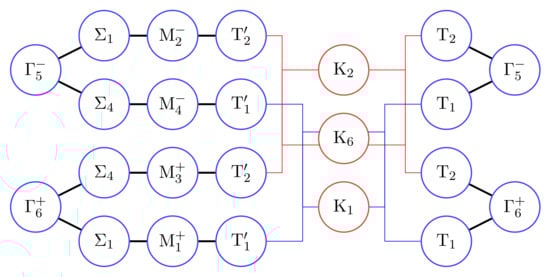
Figure 18.
Link diagram of the EBR from the spinless -orbital on Wyckoff position 2b of the honeycomb lattice. Simple links are shown in thick lines and complex links are shown in thin lines involving more than 2 nodes/terminals. All links to nodes at K are complex and their color distinguishes between the two terminals of the node .
7.2. Complex Links and Band Connectivity
The existence of a complex link associated with a node at HSPs on the surface of the BZ is a reflection of multiple unitary similarity transformations which block-diagonalize the EBR, yielding the same direct sum of invariant sub-vector spaces there. The von Neumann–Wigner (anti-crossing) theorem and dimensionality arguments would preclude links between more than two nodes/terminals. Complex links need to be resolved into unique links between two terminals at two nodes. These lead to multiple configurations of band connectivity determined solely from transformation properties of an EBR. Split EBRs [131], which are classified as decomposable [132], are included under these configurations. These configurations of band connectivity clearly reflect bands (gapped or otherwise) described by EBR bases. However, there is no indication if they correspond to an atomic limit, particularly in the gapped system.
The configurations of band connectivity corresponding to atomic limits are included as subsets of those generated by resolving complex links. From the original TQC approach, a set of connected bands described by EBR bases has an atomic limit. Implicit in such a definition is that the band described by the EBR is ‘band-invariant’ or ‘band-irreducible’, meaning the dimension of the bases and the number of connected bands are the same. This guarantees the consistency between the real space Wannier functions representation and the representation in wave vector space by the induced EBRs. If a gapped system existed under the EBR bases, the atomic limit would exist in the connected components on either side of the gap, if they were invariant/irreducible individually (guaranteed equivalence of real space Wannier function representations and induced wave vector space representations). Thus, under the TB and topological band theory, atomic limits must exist in connected bands on both sides of a gap or absent on both sides of the gap described by EBR/CBR bases. Such invariant/irreducible properties of gapped configurations of band connectivities can be tested using the projection operators in Equation (58) extended to CBR bases.
Given a system described by EBR/CBR bases, the eigenstates at the point in the BZ are well defined in terms of the bases. Those at the point can be obtained using projection operators. For a set of connected bands on one side of the gap, we can restrict in Equation (60) to those eigenstates at in the connected bands on one side of the gap. The projection operators are idempotent. For a connected band corresponding to an invariant subspace, the application of a cascade of projection operators along a closed path in the band connectivity generated by resolving a complex link must be equal to any one of them. The projection operator at a terminal at , and a cascade of operators of the form in Equations (59a) and (59b) along a closed path in configurations of connectivity should be the same for invariant/irreducible connected bands. This provides a means to identify configurations of band connectivity obtained by using projection operators corresponding to invariant subspaces. These methods of generating such configurations with an atomic limit using projection operators is equally applicable to CBR bases, provided the projection operator in Equation (58) is extended to CBR bases. Bands from different EBRs can join together on the surface of the BZ where multi-dimensional irreducible representations exist.
7.3. Band Connectivity and Band Representations
For bands described by the EBR induced from the orbital centered on Wyckoff position 2b of the honeycomb lattice, three of the possible configurations of connectivity obtained by resolving complex links are shown in Figure 19. For the totally connected configuration Figure 19b and the gapped configuration in Figure 19c, the projection operators are equivalent along closed paths. They correspond to invariant bands and the bases are band-irreducible. For the gapped configuration Figure 19a, the cascade of projection operators along closed path returns the negative of the starting operator, i.e.,
Thus, the connected bands on either side of the gap in (a) are not band-invariant and do not have IBR bases. In other words, multiple atomic limits can exist for the EBR induced from Wannier functions centered on Wyckoff positions with multiplicity. This is demonstrated in configurations (b) and (c).
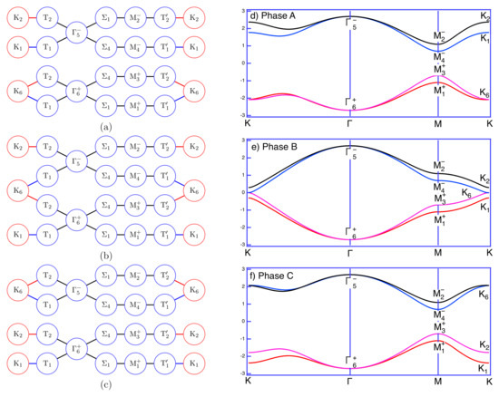
Figure 19.
Symmetry-compliant band connectivities (a–c) obtained from the projection operator method, and dispersion relations from EBRs of Wannier functions centered on Wyckoff position 2b (. The dispersion relations are obtained from the tight-binding model.
Not all configurations of band connectivity generated by resolving complex links describe invariant/irreducible bands. An example of the absence of an atomic limit is seen in the gapped system described by the PEBR induced from the spin-full orbital centered on crystallographic orbits of Wyckoff position 2b of the honeycomb lattice [127]. In this gapped case, the connected band between and breaks the equivalent nature of the cascade of projection operators along a closed path. Whilst the configuration of band connectivity is supported by the PEBR, the connected bands on each side of the gap is not invariant, and hence an atomic limit does not exist for this configuration.
The existence of complex links and the need for their resolution means there are multiple ways to block-diagonalize the representation matrix of the full EBRs at associated HSPs on the surface of the BZ. How to implement the block-diagonalization is not provided in the transformation properties of the full vector space spanned by the EBRs. Thus, transformation properties of the EBRs in the literature are incomplete in the description of energy bands and require a further context of band connectivity. When decomposable EBRs occur along orthogonal real space representations, multiple atomic limits with real space representations can exist.
The potential of the projection operator technique is also seen in an application to the configuration of connectivity obtained under the compatibility relations shown in Figure 17. For an EBR induced from the -orbitals centered on Wyckoff position 2b of the honeycomb lattice, we have
Thus, there is a simple link between and , with no link between and in the band represented by the EBR. Therefore, the configuration of the band connectivity associated with this EBR and having an atomic limit is shown in Figure 17a. Those in Figure 17b do not correspond to an atomic limit despite their compliance with compatibility relations.
The transformations of a set of connected bands are fully determined in the interior of the BZ once the symmetries of eigenstates at the point are known (compatibility relations). The makeup of these eigenstates described by an EBR can be obtained from projection operators. When the choice is made in the configuration of connectivity, the transformation properties of a connected (component) band is totally determined. For a given set of connected bands in a gapped system described by EBR/CBR bases, we define the bases of any ‘invariant/irreducible’ connected bands as ‘irreducible band representations’ (IBRs). They have real space Wannier function representations consistent with induced BRs in wave-vector space (whole connected EBR or split EBR with Wannier functions centered on a linear combination of equivalent Wyckoff positions ( index)). They can be continued to their atomic limits. In the case of a gapped system occurring due to hybridization among EBR bases (interacting EBRs), the connected bands on either side of the gap may be invariant. Whilst one cannot continue to the atomic limit due to the decoupling of the interacting EBRs in this limit, one can still show the associated Berry phase of such invariant connected bands as symmetry-forbidden under the conditions stated in Section 8. In other words, one of the important requirements of a symmetry-forbidden Berry phase is for the EBR/CBR bases describing a set of connected bands to be invariant/irreducible. The continuation to the atomic insulator prototype is not required for selection rules on the Berry phase.
Clearly, a fully connected EBR can be an IBR. This is labeled as a type 1 IBR. For the connected component of a split EBR whose transformation properties are consistent between and the surface of the BZ (having the same linear combination of EBR components in the whole BZ), its bases are labeled as a type 2 IBR. By definition, the complementary connected component must also have a real space representation, as it is orthogonal to the type 2 IBR everywhere in the BZ. The basis of the complementary connected component is also called a type 2 IBR. The consistency between and the surface of the BZ can also be achieved by hybridization. In this case, the basis of the connected component band is labeled type 3. Such a situation can be seen in the hybridization in graphene [127].
8. Symmetry Constraints on Berry Phases and Topological Invariants
One of the key outstanding issues is the equivalence between the hypothesis of TQC and the classification based on the Wilson-loop-derived topological invariants. The requirement of continuation to the atomic limit implies that the connected bands are described by the IBR bases. Thus, we can try to evaluate the Berry phase of the connected bands in terms of the IBR bases and develop selection rules for the topological invariants.
The Berry phase of a set of connected bands (they can be part of a gapped system) can be evaluated under the TB model [135]. If the connected bands are invariant/irreducible, they can be represented by their IBR bases . The energy eigenstates are related to the bases by a unitary -dependent matrix. Thus, the Berry phase in Equation (49d) can be evaluated in terms of the IBR bases and the -dependent matrix. The closed-path integral of the Berry connection (CPIBC) for invariant/irreducible connected bands is [135]
This relation holds only for the trace and only if the connected bands are invariant/irreducible. In the language of TQC, Equation (65) holds if the connected bands process an atomic limit. For connected bands which are not invariant/irreducible (they do not have IBR bases or do not have an atomic limit), one cannot develop selection rules using Equation (65). Thus, the Berry phase is not symmetry-forbidden, and the associated connected bands is symmetry-indicated as topologically non-trivial. (While this appears to be in entire agreement with definition 1 in Ref. [114], it is not the only necessary condition for a symmetry-forbidden Berry phase. The analysis based on symmetry in Section 7 goes much beyond the symmetry indicator method).
The relation in Equation (65) would hold for the connected bands with IBR bases (possibly in gapped systems). It allows the evaluation of and/or of invariant connected bands in terms of their IBR bases. Such an approach circumvents the problem associated with the non-abelian SU(N) gauge group encountered at degeneracies in multiple connected bands. However, it is not sufficient to conclude that the Berry phase and/or must be zero from this alone. Further analysis based on the transformation properties of the right-hand side of Equation (65) is required.
The transformation properties of the right-hand side of Equation (65) (without the trace) are well defined and form a representation of the group. For a space group element , this action leads to
Thus, the CPIBC with respect to the IBR bases forms a representation of the space group. The action of a space group element permutes the CPIBC among equivalent paths generated by the group element. The HSPs in the reduced zone view of the BZ is mapped onto the torus in Figure 16. The , K, and points are visible. is opposite to K along the poloidal (small circle) direction. is opposite to along the poloidal direction. is opposite to along the poloidal direction. The three different paths K-- are shown on the torus as red lines. The action of an element of a space group leads to their permutation. The closed path is uncontractible along the poloidal direction. The closed paths are uncontractible along the toroidal (large circle) direction. The only symmetry permitted form of the CPIBC with respect to the bases must transform according to the trivial representation. Therefore, one can construct the projection operator for the trivial representation and obtain the symmetry-permitted form of the CPIBC with respect to the IBR bases. This is analogous to the Wigner–Eckart theorem [133], yielding an angular-dependent part (matrix) and reduced tensor element. For a finite group, this corresponds to the general matrix element theorem developed by Koster [134]. The actual calculation is tedious, and a symmetry-permitted form always exists, yielding a symmetry-allowed Berry phase from the angular-dependent part.
However, a contractible closed path (e.g., an uncontractible path followed by its inverse) should yield a zero . In particular, if a closed path and its inverse are among the set of equivalent paths, then the sum of the two is required to be zero (contractible path). Hence, the reduced tensor element must be zero for connected bands with irreducible bases. Therefore, there are two necessary conditions for symmetry-forbidden and .
- The connected bands are invariant/irreducible, thus having IBR bases.
- The reduced tensor element of the symmetry-permitted form of the CPIBC with respect to the IBR bases is symmetry-forbidden because contractible paths should have a zero or :
The first of these two necessary conditions is closely related to the hypothesis of TQC, whereas the second one is new and dependent on the space group. This selection rule can be applied in general. In particular, the connected component band of the split EBR induced from the -orbital on Wyckoff position 2b of the honeycomb lattice with connectivity in Figure 19c has a symmetry-forbidden Berry phase. The hybridized valence band also has a symmetry-forbidden Berry phase. But the band in the gapped spin-full -orbital on Wyckoff position 2b with connected and does not have a real space representation and is therefore symmetry-indicated as non-trivial.
The Wilson loop and the Berry phase encode topological information, but their gauge dependence requires further work before the impact of symmetry can fall upon topological invariants, such as the first Chern number. In fact, the Wilson loop is one of the primary tools in assessing topological invariants. In an infinite crystal, the Berry phase itself is not significant due to gauge dependence, but its difference is well defined and has physical significance. This is similar to the commonly known polarization problem [136]. In fact, the eigenvalues of Wilson loops are named Wannier function centers. We take the 2D honeycomb lattice as an example. Consider a set of directed Wilson loops along the reciprocal lattice vector direction but with the reference point moving along the reciprocal lattice vector . This is illustrated in Figure 20. Each of the loops start along the red arrow and return with the blue arrow due to periodicity in the reciprocal space. Loops 4 and 6 have a section in green inserted between red and blue. On the torus in Figure 16, these loops run in the poloidal direction and are distributed in the toroidal direction over the whole torus. In a real calculation, one would evaluate the Wilson loop/Berry phase of all these paths. We may assign 0 and to the first and last loop, respectively. If the number of loops is increased without bound, then, in the limit, these two loops are the same, and the difference between loop 0 and loop would remove any gauge dependence. The difference in the Berry phase acquired when going from loop 0 to loop 2 returns the Chern number when two linearly independent directions are considered:
If the Berry phase as defined in Equation (49d) is symmetry-forbidden, then the only difference one acquires in the process is from the choice of gauge. This is removed in the subtraction. The Chern number is forbidden by spatial symmetry and can only take the value of zero, if the Berry phase is symmetry-forbidden. Thus, the selection rule on the Berry phase is the same as the selection rule on in this case. The situation of an EBR-induced from an s-orbital centered on Wyckoff positions 4a and 4b of the F222 space group [129] is also resolved. The system does not have a selection rule on due to the absence of a symmetry-forbidden reduced tensor element. The same applies to the Su–Schrieffer–Heeger model of conjugate polymers. One must also allow a zero in the absence of a selection rule. This may be the result of an unknown symmetry or a dynamics issue. The requirement of connected bands with continuation to the atomic limit is reduced to being invariant/irreducible and having IBR bases. This allows hybridization to be included in the development of selection rules, knowing such a system does not have an atomic limit. Many of the exceptions are incorporated in the symmetry analysis here.
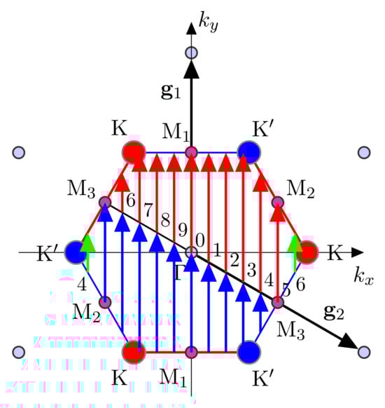
Figure 20.
A set of directed Wilson loops in the BZ of a honeycomb lattice. The direction of the loops is given by the reciprocal lattice vector , and the reference point moves along the direction of reciprocal lattice vector . The sequence traverses through the BZ. On the torus of the BZ shown in Figure 16, these loops run in the poloidal direction with the zeroth run from via and returning to . In the limit that the number of loops increases without bound, loops 0 and 9 are the same.
9. Summary
We reviewed the applications of topology in physics and their relationship to the symmetry properties of systems. As a part of this, we introduced basic concepts in topology, including topological invariants (genus and winding number), the definition of curvature, connections, and minimal surfaces. A surface with mean curvature vanishing everywhere is called a minimal surface. A minimal surface that can repeat itself along three mutually independent directions is called a triply periodic minimal surface (TPMS). Under the requirement of triple periodicity, TPMSs have a genus of at least three.
TPMSs exhibit a rich variety of applications across biology and chemistry and now extend to materials physics in martensitic phase transformations. Surfaces of zero charge density in crystals converge to TPMSs that display the symmetry and periodicity characteristic of the corresponding crystal. TPMSs describing end phases of a martensitic phase transformation have the same genus, meaning they are topologically equivalent.
Besides martensitic phase transformations, topology plays a crucial role in the study of topological materials defined by topological invariants. The topological invariants are global quantities that characterize the corresponding Bloch bundle defined on the BZ and the tangent space spanned by energy eigenstates. When there is a ‘twist’ in the band structure, there is some non-vanishing topological invariants. The first Chern number is an example of topological invariants adopted when studying topological materials in 2D systems. Berry’s phase, based on an uncontractible loop (generator of homology group), is defined generally in all dimensionality of the BZ. Chern numbers, based on integrations over all BZs (generator of homology group), are only defined in even dimensional manifold. In 3D, topological invariants are defined in terms of the Chern–Simons form. The quantization of these invariants and their value determine the characteristics of edge state and other physical properties.
The topology of energy bands in the BZ can be investigated via their homotopy-equivalent configuration of the band connectivity of their ERB/CBR bases. In particular, the configuration of the band connectivity of their EBR/CBR bases determined by symmetry alone (independent of interactions described by the Hamiltonian) correspond to those with an atomic limit. They are a subset of all symmetry-permitted configurations of band connectivity, compliant with compatibility relations and generally dependent on the Hamiltonian. Projection operators allow the identification of those configurations with an atomic limit and/or corresponding to band invariant subspaces. This facilitates the application of general matrix element theorem to the Berry phase. The symmetry analysis in Section 7 and Section 8 shows that the physically intuitive hypothesis of TQC needs modification. This is primarily due to the contradiction from a non-zero Berry phase of a band represented by the EBR induced from an s-orbital centered on Wyckoff position 4b of space group F222. Symmetry, through the general matrix element theorem, gives a well-defined topologically trivial phase in connected bands, satisfying both necessary conditions given in Section 8. Bands, with a configuration of band connectivity not homotopically equivalent to that of an IBR in the atomic limit and/or a symmetry-allowed reduced tensor element of the CPIBC with respect to the IBR bases, are symmetry-indicated as topologically non-trivial. The symmetry constraints here mean the search for topologically trivial phases should include the specification of connectivity (band-invariant properties) as well as determining if the space group yields a forbidden reduced tensor element of the CPIBC with respect to the IBR bases. The smallest building block of topologically trivial bands are IBRs, which can be an invariant subspace of the EBR induced from Wannier functions centered on Wyckoff positions with multiplicity. The current search schemes in the literature, based on the decomposition of EBRs, compatibility relations, and expansion of ‘real band structure’ from ‘EBR bases’ can incorrectly identify topologically non-trivial phase or trivial phases. The use of projection operators can correctly identify connected bands in a configuration of band connectivity corresponding to an invariant space.
Topology, a subject studying continuous deformations, interweaves with the symmetry properties of systems. Therefore, besides the previously mentioned applications of topology in physics, particularly in materials science, it is expected that topology will be applied in a wider range of research areas, thereby enriching interdisciplinary studies and offering novel insights into symmetry analyses.
Author Contributions
Writing—original draft: M.Y., D.D.V. and J.Z.; writing—review and editing: M.Y., D.D.V. and J.Z. All authors have read and agreed to the published version of the manuscript.
Funding
This research received no external funding.
Data Availability Statement
Data are available from authors’ articles cited in the review.
Conflicts of Interest
The authors declare no conflicts of interest.
Abbreviations
The following abbreviations are used in this manuscript. Number in parentheses are page numbers where abbreviations are first defined:
| TPMS | Triply periodic minimal surfaces (11) |
| DFT | Density functional theory (14) |
| BCC | Body-centered cubic (14) |
| FCC | Face-centered cubic (14) |
| ZEP | Zero equipotential surface (14) |
| RMS | Root mean square (15) |
| HCP | Hexagonal close-packed (15) |
| BZ | Brillouin zone (22) |
| RD | Representation domain (22) |
| TQC | Topological quantum chemistry (24) |
| TB | Tight binding (24) |
| BR | Band representation (24) |
| EBR | Elementary band representation (25) |
| CBR | Composite band representation (25) |
| PEBR | Physical elementary band representation (25) |
| HSP | High-symmetry point (25) |
| IBR | Irreducible band representations (31) |
| CPIBC | Closed-path integral of the Berry connection (31) |
References
- Plato. Timaeus and Critias; Lee, H.D.P., Translator; Penguin: Middlesex, UK, 1971. [Google Scholar]
- Euler, L. Solutio problematis ad geometriam situs pertinentis. Comment. Acad. Sci. Petropolitanae 1741, 8, 128–140. [Google Scholar]
- James, I.M. (Ed.) History of Topology; Elsevier: Amsterdam, The Netherlands, 1999. [Google Scholar]
- Cantor, G. Üeber unendliche, lineare Punktmannichfaltigkeiten. Math. Ann. 1883, 21, 545–591. [Google Scholar] [CrossRef]
- Hausdorff, F. Grundzüge der Mengenlehre; Leipzig Viet: Leipzig, Germany, 1914. [Google Scholar]
- Yang, C.N. Quantum numbers, Chern classes, and a bodhisattva. Phys. Today 2012, 65, 33–34. [Google Scholar] [CrossRef]
- Yang, C.N. Topology and gauge theory in physics. Int. J. Mod. Phys. A 2012, 27, 1230035. [Google Scholar] [CrossRef]
- Avron, J.E.; Osadchy, D.; Seiler, R. A topological look at the quantum Hall effect. Phys. Today 2003, 56, 38–42. [Google Scholar] [CrossRef]
- Thouless, D.J.; Kohmoto, M.; Nightingale, M.P.; den Nijs, M. Quantized Hall conductance in a two-dimensional periodic potential. Phys. Rev. Lett. 1982, 49, 405–408. [Google Scholar] [CrossRef]
- Hyde, S.; Andersson, S. A cubic structure consisting of a lipid bilayer forming an infinite periodic minimum surface of the gyroid type in the glycerolmonooleat-water system. Z. Kristallogr. Cryst. Mater. 1984, 168, 213–220. [Google Scholar] [CrossRef]
- Hyde, S.; Andersson, S. Differential geometry of crystal structure descriptions, relationships and phase transformation. Z. Kristallogr. Cryst. Mater. 1985, 170, 225–240. [Google Scholar] [CrossRef]
- Hyde, S.; Andersson, S. The martensite transition and differential geometry. Z. Kristallogr. Cryst. Mater. 1986, 174, 225–236. [Google Scholar] [CrossRef]
- Andersson, S.; Hyde, S.; Larsson, K.; Lidin, S. Minimal Surfaces and Structures: From Inorganic and Metal Crystals to Cell Membranes and Biopolymers. Chem. Rev. 1988, 88, 221–242. [Google Scholar] [CrossRef]
- Anirban, A. 15 years of topological matter. Nat. Rev. Phys. 2023, 5, 267. [Google Scholar] [CrossRef]
- Wang, J.; Zhang, S.C. Topological states of condensed matter. Nat. Mater. 2017, 16, 1062–1067. [Google Scholar] [CrossRef]
- Pariari, A.K. Atoms to Topological Electronic Materials: A Bedtime Story for Beginners. Indian J. Phys. 2021, 95, 2636–2660. [Google Scholar] [CrossRef]
- Gao, H.; Venderbos, J.W.F.; Kim, Y.; Rappe, A.M. Topological semimetals from first principles. Annu. Rev. Mater. Res. 2019, 49, 153–183. [Google Scholar] [CrossRef]
- Yan, B.; Felser, C. Topological materials: Weyl semimetals. Annu. Rev. Mater. Res. 2017, 8, 337–354. [Google Scholar] [CrossRef]
- Lv, B.Q.; Qian, T.; Ding, H. Experimental perspective on three-dimensional topological semimetals. Rev. Mod. Phys. 2021, 93, 025002. [Google Scholar] [CrossRef]
- Shen, S.Q. The family of topological phases in condensed matter. Natl. Sce. Rev. 2017, 1, 49–59. [Google Scholar] [CrossRef]
- Zhang, Y.; Wang, Y.; Liu, Y. Topology optimization: A review for structural designs under static problems. Materials 2024, 17, 5970. [Google Scholar] [CrossRef]
- Ghil, M. Review article: Dynamical systems, algebraic topology and the climate sciences. Nonlin. Process. Geophys. 2023, 30, 399–434. [Google Scholar] [CrossRef]
- Garcia, M.S.; Süsstrunk, R.; Huber, S.D. Topology in nonlinear mechanical systems. Phys. Rev. Lett. 2021, 127, 076802. [Google Scholar] [CrossRef]
- Shankar, S.; Bowick, S.M.J.; Marchetti, M.C.; Vitelli, V. Topological active matter. Nat. Rev. Phys. 2022, 4, 380–398. [Google Scholar] [CrossRef]
- Gross, D.J. The role of symmetry in fundamental physics. Proc. Natl. Acad. Sci. USA 1996, 93, 14256–14259. [Google Scholar] [CrossRef] [PubMed]
- Senthil, T. Symmetry-protected topological phases of quantum matter. Annu. Rev. Condens. Matter. Phys. 2015, 6, 299–324. [Google Scholar] [CrossRef]
- Fischer, M.H.; Sigrist, M.; Agterberg, D.F.; Yanase, Y. Superconductivity and local inversion-symmetry breaking. Annu. Rev. Condens. Matter. Phys. 2023, 14, 153–172. [Google Scholar] [CrossRef]
- McGrevy, J. Generalized symmetries in condensed matter. Annu. Rev. Condens. Matter. Phys. 2023, 14, 57–82. [Google Scholar] [CrossRef]
- Nakahara, M. Geometry Topology and Physics; IOP Publishing Ltd.: West Philadelphia, PA, USA, 2003. [Google Scholar]
- Hasan, M.; Kane, C. Colloquium: Topological insulators. Rev. Mod. Phys. 2010, 82, 3045–3067. [Google Scholar] [CrossRef]
- Qi, X.; Zhang, S. Topological insulators and superconductors. Rev. Mod. Phys. 2011, 83, 1057–1110. [Google Scholar] [CrossRef]
- Murakami, S.; Hirayama, M.; Okugawa, R.; Miyake, T. Emergence of topological semimetals in gap closing in semiconductors without inversion symmetry. Sci. Adv. 2017, 3, e1602680. [Google Scholar] [CrossRef]
- Burkov, A.A. Topological semimetals. Nat. Mater. 2016, 15, 1145–1148. [Google Scholar] [CrossRef]
- Yu, R.; Weng, H.; Fang, Z.; Dai, X.; Hu, X. Topological node-line semimetal and Dirac semimetal state in antiperovskite Cu3PdN. Phys. Rev. Lett. 2015, 115, 036807. [Google Scholar] [CrossRef]
- Burkov, A.A.; Hook, M.D.; Balents, L. Topological nodal semimetals. Phys. Rev. B 2011, 84, 235126. [Google Scholar] [CrossRef]
- Mermin, N.D. The topological theory of defects in ordered media. Rev. Mod. Phys. 1979, 51, 591–648. [Google Scholar] [CrossRef]
- Michel, L. Symmetry defects and broken symmetry. Configurations Hidden symmetry. Rev. Mod. Phys. 1980, 52, 617–651. [Google Scholar] [CrossRef]
- Munkres, J. Topology; Prentice Hall: Upper Saddle River, NJ, USA, 2000. [Google Scholar]
- Carmo, M. Differential Geometry of Curves and Surfaces; Dover: New York, NY, USA, 2016. [Google Scholar]
- Sethna, J.P. Frustration and curvature: Glasses and the cholesteric blue phase. Phys. Rev. Lett. 1983, 51, 2198–2201. [Google Scholar] [CrossRef]
- Rosso, R.; Virga, E.G.; Kralj, S. Parallel transport and defects on nematic shells. Contin. Mech. Thermodyn. 2012, 24, 643–664. [Google Scholar] [CrossRef]
- Brazil, R. Fighting flat-Earth theory. Phys. World 2020, 33, 35–39. [Google Scholar] [CrossRef]
- Dreshler, W.; Mayer, M.E. Fiber Bundle Techniques in Gauge Theories: Lectures in Mathematical Physics at the University of Texas at Austin: 67; Lecture Notes in Physics, 67; Springer: Berlin, Germany, 1977. [Google Scholar]
- Cayssol, J.; Fuchs, J.N. Topological and geometrical aspects of band theory. J. Phys. Mater. 2021, 4, 034007. [Google Scholar] [CrossRef]
- Fruchart, M.; Carpentier, D. An introduction to topological insulators. Comptes Rendus Phys. 2013, 14, 779–815. [Google Scholar] [CrossRef]
- Hillel, D. (Ed.) Encyclopedia of Soils in the Environment; Academic Press: Los Angeles, CA, USA, 2005. [Google Scholar]
- Schwarz, H.A. Gesammelte Mathematische Abhandlungen; American Mathematical Society: Ann Arbor, MI, USA, 1972. [Google Scholar]
- Lai, M.; Kulak, A.; Law, D.; Zhang, Z.; Meldrum, F.; Riley, D. Profiting from nature: Macroporous copper with superior mechanical properties. Chem. Commun. 2007, 34, 3547–3549. [Google Scholar] [CrossRef]
- Galusha, J.; Richey, L.; Gardner, J.; Cha, J.; Bartl, M. Discovery of a diamond-based photonic crystal structure in beetle scales. Phys. Rev. E 2008, 77, 050904. [Google Scholar] [CrossRef]
- Feng, J.; Fu, J.; Yao, X.; He, Y. Triply periodic minimal surface (TPMS) porous structures: From multi-scale design, precise additive manufacturing to multidisciplinary applications. Int. J. Extrem. Manuf. 2022, 4, 022001. [Google Scholar] [CrossRef]
- Pugliesea, R.; Graziosib, S. Biomimetic scaffolds using triply periodic minimal surface-based porous structures for biomedical applications. SLAS Technol. 2023, 28, 165–182. [Google Scholar] [CrossRef] [PubMed]
- Huang, Y.; Zhai, L. Structural optimization, compressive strength analysis, and application exploration of triply periodic minimal surfaces (TPMS) in interior design. Sci. Rep. 2025, 15, 11026. [Google Scholar] [CrossRef] [PubMed]
- Cheung, S.; Kang, J.; Lin, Y.; Goodson, K.E.; Asheghi, M.; Gu, X.W. Triply periodic minimal surfaces for thermo-mechanical protection. Sci. Rep. 2025, 15, 1688. [Google Scholar] [CrossRef]
- Gado, M.G.; Al-Ketan, O.; Aziz, M.; Al-Rub, R.A.; Ookawara, S. Triply periodic minimal surface structures: Design, fabrication, 3D printing techniques, state-of-the-art studies, and prospective thermal applications for efficient energy utilization. Energy Technol. 2024, 12, 2301287. [Google Scholar] [CrossRef]
- Felix, L.C.; Ambekar, R.; Tromer, R.M.; Woellner, C.F.; Rodrigues, V.; Ajayan, P.M.; Tiwary, C.S.; Galvao, D.S. Schwarzites and triply periodic minimal surfaces: From pure topology mathematics to macroscale applications. Small 2024, 2400351. [Google Scholar] [CrossRef]
- Fomenko, A.; Tuzhilin, A. Elements of the Geometry and Topology of Minimal Surfaces in Three-Dimensional Space; American Mathematical Society: Ann Arbor, MI, USA, 2000. [Google Scholar]
- Weierstrass, K. Mathematische Werke; Mayer & Müller: Berlin, Germany, 1903. [Google Scholar]
- Enneper, A. Analytisch-Geometrische Untersuchung. Z. Math. Phys. 1864, 9, 96–125. [Google Scholar]
- Schoen, A.H. Infinite Periodic Minimal Surfaces without Self-Intersections; Tech. Rep. TN D-5541; NASA: Washington, DC, USA, 1970. [Google Scholar]
- Osmond, F. Nomenclature in Metallography. J. Iron Steel Inst. 1902, 61, 90. [Google Scholar]
- Portella, P.D.; Helmerich, R. Adolf Martens and his contribution to materials engineering. Eng. Fail. Anal. 2014, 43, 2–10. [Google Scholar] [CrossRef]
- Hao, Y.; Zhang, L.; Chen, X.; Cai, L.; Wu, Q.; Alfè, D. Ab initio calculations of the thermodynamics and phase diagram of zirconium. Phys. Rev. B 2008, 78, 134101. [Google Scholar] [CrossRef]
- Campbell, W. Twenty-five years of metallography, 3rd Howe Memorial Award. Trans. AIME 1926, 73, 1135. [Google Scholar]
- Greninger, A.; Mooradian, V. Strain transformation in metastable beta copper-zinc and beta copper-titanium alloys. Trans. AIME 1938, 128, 337. [Google Scholar]
- Wadhawan, V. Ferroelasticity and related properties of crystals. Phase Transit. 1982, 3, 3–103. [Google Scholar] [CrossRef]
- Buehler, W.; Gilfrich, J.; Wiley, R. Effect of low-temperature phase changes on the mechanical properties of alloys near composition TiNi. J. Appl. Phys. 1963, 34, 1475–1477. [Google Scholar] [CrossRef]
- Hatcher, N.; Kontsevoi, O.; Freeman, A. Martensitic transformation path of NiTi. Phys. Rev. B 2009, 79, 020202(R). [Google Scholar] [CrossRef]
- Hatcher, N.; Kontsevoi, O.; Freeman, A. Role of elastic and shear stabilities in the martensitic transformation path of NiTi. Phys. Rev. B 2009, 80, 144203. [Google Scholar] [CrossRef]
- Mishin, Y.; Farkas, D.; Mehl, M.; Papaconstantopoulos, D. Interatomic potentials for monoatomic metals from experimental data and ab initio calculations. Phys. Rev. B 1999, 59, 3393–3407. [Google Scholar] [CrossRef]
- Wang, T.; Du, J.; Wei, S.; Liu, F. Ab-initio investigation for the microscopic thermodynamics and kinetics of martensitic transformation. Prog. Nat. Sci. Mater. 2021, 31, 121–128. [Google Scholar] [CrossRef]
- Zhang, L.; Cheng, M.; Shi, X.; Shuai, J.; Zhu, Z. Bain and Nishiyama–Wassermann transition path separation in the martensitic transitions of Fe. RSC Adv. 2021, 11, 3043. [Google Scholar] [CrossRef]
- Kibey, S.; Sehitoglu, H.; Johnson, D. Energy landscape for martensitic phase transformation in shape memory NiTi. Mater. Res. Soc. Symp. Proc. 2009, 57, 1624–1629. [Google Scholar] [CrossRef]
- Chakraborty, T.; Rogal, J.; Drautz, R. Martensitic transformation between competing phases in Ti–Ta alloys: A solid-state nudged elastic band study. J. Phys. Condens. Matter. 2015, 27, 115401. [Google Scholar] [CrossRef]
- Ghosh, P.; Arya, A.; Tewari, R.; Dey, G. Alpha to omega martensitic phase transformation pathways in pure Zr. J. Alloys Compd. 2014, 586, 693–698. [Google Scholar] [CrossRef]
- Trinkle, D.; Hatch, D.; Stokes, H.; Hennig, R.; Albers, R. Systematic pathway generation and sorting in martensitic transformations: Titanium alpha to omega. Phys. Rev. B 2005, 72, 014105. [Google Scholar] [CrossRef]
- Cowley, R. Structural phase transitions I. Landau theory. Adv. Phys. 1980, 29, 1–110. [Google Scholar] [CrossRef]
- Pallikara, I.; Skelton, J. Phase stability of the tin monochalcogenides SnS and SnSe: A quasi-harmonic lattice-dynamics study. Phys. Chem. Chem. Phys. 2021, 23, 19219. [Google Scholar] [CrossRef]
- Pallikara, I.; Kayastha, P.; Skelton, J.; Whalley, L. The physical significance of imaginary phonon modes in crystals. Electron. Struct. 2022, 4, 033002. [Google Scholar] [CrossRef]
- Kamba, S. Soft-mode spectroscopy of ferroelectrics and multiferroics: A review. APL Mater. 2021, 9, 020704. [Google Scholar] [CrossRef]
- Scott, J.F. Soft-mode spectroscopy: Experimental studies of structural phase transitions. Rev. Mod. Phys. 1974, 46, 83–128. [Google Scholar] [CrossRef]
- Tolédano, J.; Tolédano, P. The Landau Theory of Phase Transitions; World Scientific: River Edge, NJ, USA, 1987. [Google Scholar]
- Tolédano, P.; Dmitriev, V. Reconstructive Phase Transitions: In Crystals and Quasicrystals; World Scientific: River Edge, NJ, USA, 1996. [Google Scholar]
- Landau, L.; Lifshitz, E. Course of Theoretical Physics, Statistical Physics; Pergamon Press: Oxford, UK, 1980. [Google Scholar]
- Falk, F. Model free energy, mechanics, and thermodynamics of shape memory alloys. Acta Mater. 1980, 28, 1773–1780. [Google Scholar] [CrossRef]
- Falk, F. Landau theory and martensitic phase transitions. J. Phys. Colloq. 1982, 43, C4-3–C4-15. [Google Scholar] [CrossRef]
- Nesper, R.; Schnering, H. Periodische äquipotential flächen. Z. Kristallogr. 1985, 170, 138. [Google Scholar]
- Schnering, H.; Nesper, R. How nature adapts chemical structures to curved surfaces. Angew. Chem. 1987, 26, 1059–1080. [Google Scholar] [CrossRef]
- Schnering, H.; Nesper, R. Nodal surfaces of Fourier series: Fundamental invariants of structured matter. Z. Physik B Condensed Matter. 1991, 83, 407–412. [Google Scholar] [CrossRef]
- Yin, M.; Zhang, J.; Vvedensky, D.D. Density-functional theory and triply-periodic minimal surfaces. arXiv 2025, arXiv:2503.12555. [Google Scholar] [CrossRef]
- Kittel, C. Introduction to Solid State Physics, 8th ed.; John Wiley & Sons, Inc.: Hoboken, NJ, USA, 2005. [Google Scholar]
- Yin, M.; Vvedensky, D.D. Shape memory effect and the topology of minimal surfaces. Symmetry 2024, 16, 1187. [Google Scholar] [CrossRef]
- Berry, M.V. Quantal phase factors accompanying adiabatic changes. Proc. R. Soc. Lond. A 1984, 392, 45–57. [Google Scholar] [CrossRef]
- Simon, B. Holonomy, the quantum adiabatic theorem, and Berry’s phase. Phys. Rev. Lett. 1983, 51, 2167–2170. [Google Scholar] [CrossRef]
- Zwanziger, J.W.; Koenig, M.; Pines, A. Berry’s phase. Annu. Rev. Phys. Chem. 1990, 41, 601–646. [Google Scholar] [CrossRef]
- Xiao, D.; Chang, M.-C.; Niu, Q. Berry phase effects on electronic properties. Rev. Mod. Phys. 2010, 82, 1959–2007. [Google Scholar] [CrossRef]
- Girvin, S.M.; Yang, K. Modern Condensed Matter Physics; Cambridge University Press: Cambridge, UK, 2019. [Google Scholar]
- Messiah, A. Quantum Mechanics; North-Holland: Amsterdam, The Netherlands, 1962; Volume II. [Google Scholar]
- Fu, L.; Kane, C.L. Topological insulators with inversion symmetry. Phys. Rev. B 2007, 76, 045302. [Google Scholar] [CrossRef]
- Liu, G.; Gao, Z.; Zhang, B. Topological Chern vectors in three-dimensional photonic crystals. Nature 2022, 609, 925–930. [Google Scholar] [CrossRef] [PubMed]
- Weinberg, S. Lectures on Quantum Mechanics, 2nd ed.; Cambridge University Press: Cambridge, UK, 2015. [Google Scholar]
- Asbóth, J.K.; Oroszlány, L.; Pályi, A. A Short Course on Topological Insulators; Springer: Cham, Switzerland, 2016. [Google Scholar]
- Hatsugai, Y. Chern number and edge states in the integer quantum Hall effect. Phys. Rev. Lett. 1993, 71, 3697–3700. [Google Scholar] [CrossRef] [PubMed]
- Johnsen, T.; Schattauer, C.; Samaddar, S.; Weston, A.; Hamer, M.J.; Watanabe, K.; Taniguchi, T.; Gorbachev, R.; Libisch, F.; Morgenstern, M. Mapping quantum Hall edge states in graphene by scanning tunneling microscopy. Phys. Rev. B 2023, 107, 115426. [Google Scholar] [CrossRef]
- Halperin, B.I. Quantized Hall conductance, current-carrying edge states, and the existence of extended states in a two-dimensional disordered potential. Phys. Rev. B 1982, 25, 2185–2190. [Google Scholar] [CrossRef]
- Kane, C.L.; Mele, E.J. Quantum spin Hall effect in graphene. Phys. Rev. Lett. 2005, 95, 226801. [Google Scholar] [CrossRef]
- Bernevig, B.A.; Hughes, T.L.; Zhang, S.-C. Quantum spin Hall effect and topological phase transition in HgTe quantum wells. Science 2006, 314, 1757–1761. [Google Scholar] [CrossRef]
- Kitaev, A.Y. Unpaired Majorana fermions in quantum wires. Phys. Usp. 2001, 44, 131–136. [Google Scholar] [CrossRef]
- Fu, L.; Kane, C.L. Superconducting proximity effect and Majorana Fermions at the surface of a topological insulator. Phys. Rev. Lett. 2008, 100, 096407. [Google Scholar] [CrossRef]
- Wilczek, F.; Zee, A. Appearance of Gauge Structure in Simple Dynamical Systems. Phys. Rev. Lett. 1984, 52, 2111–2114. [Google Scholar] [CrossRef]
- Marcel, F.; Laurens, M. (Eds.) Topological Insulators. In Contemporary Concepts in Condensed Matter Science; Elsevier B.V.: Amsterdam, The Netherlands, 2013; Volume 6. [Google Scholar]
- Bradlyn, B.; Iraola, M. Lecture notes on Berry phases and topology. Scipost Phys. Lect. Notes 2022, 51, 51. [Google Scholar] [CrossRef]
- Bradley, C.J.; Davies, B.L. Magnetic groups and their corepresentations. Rev. Mod. Phys. 1968, 40, 359–379. [Google Scholar] [CrossRef]
- Kane, C.L.; Mele, E.J. Z2 topological order and the quantum spin hall effect. Phys. Rev. Lett. 2005, 95, 146802. [Google Scholar] [CrossRef] [PubMed]
- Bradlyn, B.; Elcoro, L.; Cano, J.; Vergniory, M.G.; Wang, Z.; Felser, C.; Aroyo, M.I.; Bernevig, B.A. Topological quantum chemistry. Nature 2017, 547, 298–305. [Google Scholar] [CrossRef]
- Po, H.; Vishwanath, A.; Watanabe, H. Symmetry-based indicators of band topology in the 230 space groups. Nature Commu. 2017, 8, 50. [Google Scholar] [CrossRef]
- Kruthoff, J.; de Boer, J.; van Wezel, J.; Kane, C.L.; Slager, R.-J. Topological classification of crystalline insulators through band structure combinatorics. Phys. Rev. X 2017, 7, 041069. [Google Scholar] [CrossRef]
- Wannier, G.H. The structure of electronic excitation levels in insulating crystals. Phys. Rev. 1936, 52, 191–197. [Google Scholar] [CrossRef]
- Marzari, N.; Mostofi, A.A.; Yates, J.R.; Souza, I.; Vanderbilt, D. Maximally localized Wannier functions: Theory and applications. Rev. Mod. Phys. 2012, 84, 1419–1475. [Google Scholar] [CrossRef]
- Slater, J.; Koster, G. Simplified LCAO method for the periodic potential problem. Phys. Rev. 1954, 94, 1498–1524. [Google Scholar] [CrossRef]
- Zak, J. Band representations of space groups. Phys. Rev. B 1982, 26, 3010–3023. [Google Scholar] [CrossRef]
- Cano, J.; Bradlyn, B.; Wang, Z.; Elcoro, L.; Vergniory, M.G.; Felser, C.; Aroyo, M.I.; Bernevig, B.A. Building blocks of topological quantum chemistry: Elementary band representations. Phys. Rev. B 2018, 97, 035139. [Google Scholar] [CrossRef]
- Cano, J.; Bradlyn, B. Band representations and topological quantum chemistry. Annu. Rev. Condens. Matter Phys. 2021, 12, 225–246. [Google Scholar] [CrossRef]
- Evarestov, R.A. Quantum Chemistry of Solids: The LCAO First Principles Treatment of Crystals; Springer Series in Solid-State Sciences; Springer: Berlin/Heidelberg, Germany, 2007. [Google Scholar] [CrossRef]
- Zak, J. Continuity chords of bands in solids: The diamond structure. Phys. Rev. B 1982, 25, 1344. [Google Scholar] [CrossRef]
- Bouckaert, L.; Smoluchowski, R.; Wigner, E. Theory of Brillouin zones and symmetry properties of wave functions in crystals. Phys. Rev. 1936, 50, 58–67. [Google Scholar] [CrossRef]
- Vergniory, M.G.; Elcoro, L.; Wang, Z.; Cano, J.; Felser, C.; Aroyo, M.I.; Bernevig, B.A.; Bradlyn, B. Graph theory data for topological quantum chemistry. Phys. Rev. E 2017, 95, 023310. [Google Scholar] [CrossRef]
- Zhang, J. Band representation, band connectivity and irreducibility. arXiv 2021, arXiv:2109.15219. [Google Scholar] [CrossRef]
- Po, H.C. Symmetry indicators of band topology. J. Phys. C Cond. Matt. 2020, 32, 263001. [Google Scholar] [CrossRef]
- Cano, J.; Elcoro, L.; Aroyo, M.I.; Bernevig, B.A.; Bradlyn, B. Topology invisible to eigenvalues in obstructed atomic insulators. Phys. Rev. B 2022, 105, 125115. [Google Scholar] [CrossRef]
- Bacry, H.; Michel, L.; Zak, J. Symmetry and Analyticity of Energy Bands in Solids. Phys. Rev. Lett. 1988, 61, 1005–1008. [Google Scholar] [CrossRef]
- Cano, J.; Bradlyn, B.; Wang, Z.; Elcoro, L.; Vergniory, M.G.; Felser, C.; Aroyo, M.I.; Bernevig, B.A. Topology of D disconnected elementary band representations. Phys. Rev. Lett. 2018, 120, 266401. [Google Scholar] [CrossRef]
- Elcoro, L.; Bradlyn, B.; Wang, Z.; Vergniory, M.G.; Cano, J.; Felser, C.; Bernevig, B.A.; Orobengoa, D.; de la Flor, G.; Aroyo, M.I. Double crystallographic groups and their representations on the Bilbao crystallographic server. J. Appl. Crystal. 2017, 50, 1457–1477. [Google Scholar] [CrossRef]
- Eckart, C. The application of group theory to the quantum dynamics of monatomic systems. Rev. Mod. Phys. 1930, 2, 305–380. [Google Scholar] [CrossRef]
- Koster, G. Matrix elements of symmetric operators. Phys. Rev. 1958, 109, 227–231. [Google Scholar] [CrossRef]
- Zhang, J. Symmetry constraints on topological invariants and irreducible band representations. arXiv 2024, arXiv:2408.16658. [Google Scholar] [CrossRef]
- Resta, R. Theory of electrical polarization in crystals. Ferroelectrics 1992, 136, 51–55. [Google Scholar] [CrossRef]
Disclaimer/Publisher’s Note: The statements, opinions and data contained in all publications are solely those of the individual author(s) and contributor(s) and not of MDPI and/or the editor(s). MDPI and/or the editor(s) disclaim responsibility for any injury to people or property resulting from any ideas, methods, instructions or products referred to in the content. |
© 2025 by the authors. Licensee MDPI, Basel, Switzerland. This article is an open access article distributed under the terms and conditions of the Creative Commons Attribution (CC BY) license (https://creativecommons.org/licenses/by/4.0/).