A BiGRUSA-ResSE-KAN Hybrid Deep Learning Model for Day-Ahead Electricity Price Prediction

Abstract

In the context of the clean and low-carbon transformation of power systems, addressing the challenge of day-ahead electricity market price prediction issues triggered by the strong stochastic volatility of power supply output due to high-penetration renewable energy integration, as well as problems such as limited dataset scales and short market cycles in test sets associated with existing electricity price prediction methods, this paper introduced an innovative prediction approach based on a multi-modal feature fusion and BiGRUSA-ResSE-KAN deep learning model. In the data preprocessing stage, maximum–minimum normalization techniques are employed to process raw electricity price data and exogenous variable data; the complete ensemble empirical mode decomposition with adaptive noise (CEEMDAN) and variational mode decomposition (VMD) methods are utilized for multi-modal decomposition of electricity price data to construct a multi-scale electricity price component matrix; and a sliding window mechanism is applied to segment time-series data, forming a three-dimensional input structure for the model. In the feature extraction and prediction stage, the BiGRUSA-ResSE-KAN multi-branch integrated network leverages the synergistic effects of gated recurrent units combined with residual structures and attention mechanisms to achieve deep feature fusion of multi-source heterogeneous data and model complex nonlinear relationships, while further exploring complex coupling patterns in electricity price fluctuations through the knowledge-adaptive network (KAN) module, ultimately outputting 24 h day-ahead electricity price predictions. Finally, verification experiments conducted using test sets spanning two years from five major electricity markets demonstrate that the introduced method effectively enhances the accuracy of day-ahead electricity price prediction, exhibits good applicability across different national electricity markets, and provides robust support for electricity market decision making.

1. Introduction

Against the macro-background of the global active practice of the concept of sustainable development, countries have to implement emission reduction policies to drive the transformation of low-carbon economy, accelerating its energy structure to green the direction of the depth of the transition [1]. As the main force of carbon emissions, the electric power industry has an important mission in the transition. With the global implementation of the Paris Agreement progressing [2,3], countries are increasing their efforts to reduce emissions and strengthening energy cooperation. Consequently, the pace of constructing the global electricity market has accelerated. As the core of market transactions, accurately grasping the direction of industry marketization is of crucial importance [4]. Electricity price, as the core price signal of the complex electricity market system, has a formation mechanism that is essentially the macro-equilibrium result emerging through the competitive bidding game between market entities on both the supply and demand sides [5]. Recently, the clearing of market electricity prices has been a key link in the electricity spot market trading system, which has a pronounced impact on the dispatching decisions of the power system, the bidding strategies of power generation enterprises, the formulation of users’ electricity purchase plans, and real-time market transactions. Improving the accuracy of electricity price prediction not only helps optimize the dispatching and operation mode of the power system but also provides data support for power generation enterprises to formulate more reasonable unit bidding strategies. At the same time, it is beneficial for the user side to set power purchase plans more accurately and further affects the transaction efficiency of the real-time market [6].

Spot electricity prices are comprehensively influenced by multiple factors. Their sequence presents multi-scale frequency domain characteristics, consisting of high-frequency signals reflecting unexpected events or weather changes, medium-frequency signals reflecting intraday periodic fluctuations, and low-frequency signals revealing seasonal trends and long-term policy impacts. They are characterized by nonstationarity, periodicity, and complex volatility and are difficult to predict [7]. To address these challenges, deep learning methods have gradually become a research hotspot and have been widely applied in this field. Work [8] constructed a graph model to describe the geographically distributed electricity market data and extracted extraterritorial information with the help of the graph convolution network (GCN). After integrating this information into a time series and inputting it into the long short-term memory (LSTM) network, the marginal electricity price of the day-ahead market is predicted. Work [5] introduced a short-term electricity market price prediction model combining singular spectrum analysis (SSA), convolutional neural network (CNN), and gated recursive unit (GRU), which utilizes the SSA to decompose and reconstruct the original data, the CNN to extract the high-dimensional features, the GRU to build the feature dynamics model, and finally obtains the prediction results through the cumulative prediction sequences, thus improving the prediction accuracy. Work [9] introduced a method based on ATT-CNN-LSTM to improve the prediction accuracy and efficiency of short-term electricity prices at jump points and peak points. That is, the grey correlation degree is used to screen the associated load data, the weights are allocated with the help of the attention mechanism, and then feature extraction and dimension reduction are carried out through the CNN to optimize the LSTM input. This method has been verified to be superior in the Australian market. Work [10] introduced a prediction framework integrating Loess seasonal trend decomposition, GRU, lightweight gradient lift, and Shapley additive interpretation, which was effectively verified in the electricity markets of the United States and Australia.

Although the existing deep learning methods have achieved certain results in electricity price prediction, the model structure is often complex, the parameters are redundant, and the nonlinear modeling ability is insufficient. Especially, the ability to capture high-frequency sudden change signals is weak. At the same time, they lack interpretability and weaken the value of decision support. The Kolmogorov–Arnold networks (KANs) [11] directly fit multi-scale features with adaptive spline functions, effectively reducing parameter redundancy and significantly improving training efficiency while ensuring high prediction accuracy. Furthermore, their spline structure has strong interpretability and can clearly analyze the relationships among variables, such as accurately presenting seasonal trends and the impact of extreme events on the electricity market, providing a transparent and reliable basis for electricity market decision making. Work [12] introduced a residual electricity price prediction method based on the KAN module with a learnable activation function and transferring learning from points to edges, which is more sensitive to features. The activation function is constructed through discrete Fourier transform to achieve the prediction of electricity prices in the Australian national electricity market 30 min before the current day, effectively reducing the impact of pronounced price fluctuations and ensuring the stability of learning. Work [7] introduced a heterogeneous deep learning integrated prediction method fusing a reconstruction-based quadratic decomposition–integration framework with the KAN algorithm to decompose the spot tariff signal using the RSDE framework, followed by a deep learning model of the KAN algorithm to model and predict the reconstructed subsequences in different frequency domains, and then finally adaptive weighted regression to integrate the results to improve the tariff prediction accuracy, which is empirically demonstrated to outperform the baseline model.

Facing the current highly complex and fluctuating electricity prices, all kinds of prediction models have certain limitations. However, various advanced hybrid models have been widely introduced and applied in current research. Among them, the decomposition technology, as the core branch of the hybrid model, has been adopted by many researchers because it can reduce nonstationarity and extract multi-scale features to improve the prediction accuracy. Common mode decomposition methods include empirical mode decomposition (EMD) [13], ensemble empirical mode decomposition (EEMD) [14,15], VMD [16], improved complete ensemble empirical mode decomposition with adaptive noise (ICEEMDAN) [17], and SSA [18]. However, when single-modal decomposition is used for multi-scale decomposition of electricity prices with sharp changes, modal aliasing and false components are prone to occur, resulting in the omission or redundancy of scale features. Meanwhile, secondary decomposition is likely to make the multi-scale component levels obtained from the second layer decomposition too deep, thereby making it difficult to extract the weak features of some scale signals [6]. Work [19] uses the VMD-EEMD-LSTM model to forecast rebar futures prices, employing VMD and EEMD for data preprocessing and using MAE, RMSE, and MAPE metrics to assess its predictive performance against other models. Work [6] introduced an ultrashort-term wind power prediction model, which utilizes wavelet decomposition (WD) and VMD to double decompose the wind power sequence into modal components, and then the prediction is performed by multiple least-squares support vector machine (LSSVM) models, which are finally fused to obtain the wind power prediction results.

Although the electricity price prediction technology that integrates time-series analysis and deep learning models has made certain progress, the current method still faces many challenges. Specifically, the integration of the hybrid deep learning model architecture is not sufficient, and the dataset on which the prediction relies is relatively single, resulting in poor comprehensiveness of the model demonstration. Meanwhile, the prediction model has deficiencies in the adaptability assessment for multiple electricity markets, and the test set has a short time span, making it difficult to cover the entire year cycle. These factors collectively constrain the model’s capacity to respond promptly to electricity price fluctuations in real-world scenarios. Based on the above analysis, this study introduced an innovative electricity price prediction method:

• In this study, we systematically solve the core challenge of asymmetry of day-ahead tariff prediction intervals under a high percentage of renewable energy grid-connectedness by constructing a symmetric adaptive prediction framework. Based on the innovative design of multi-modal feature fusion and BiGRUSA-ResSE-KAN deep learning architecture, we realize the dual balance of prediction accuracy and interval symmetry.
• A novel hybrid approach combining CEEMDAN and VMD is employed to decompose electricity price data into multi-scale components. This method reorganizes components by frequency, constructing a multi-scale matrix that effectively captures fluctuation patterns and lays a foundation for deep feature extraction.
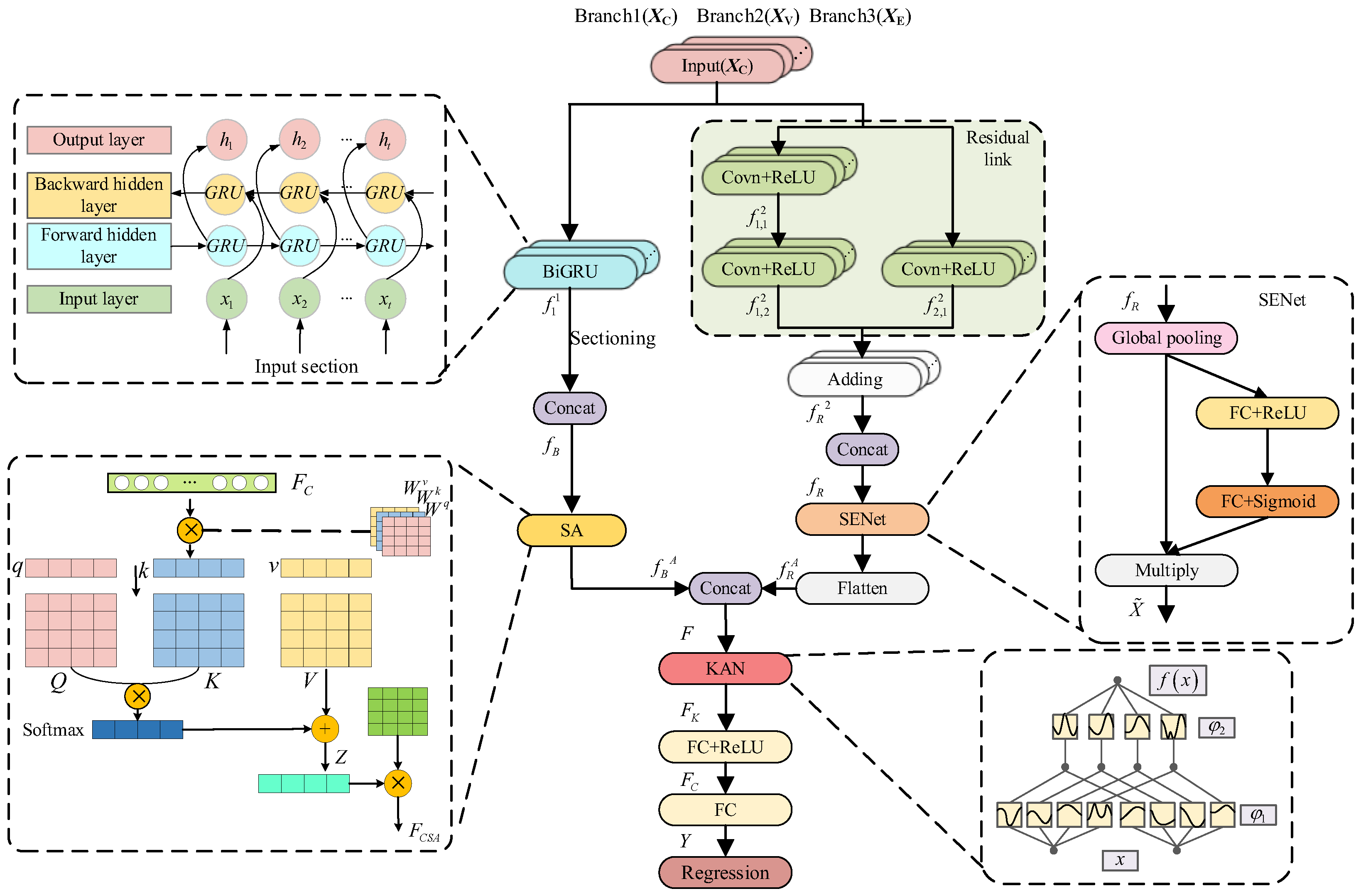
• The introduced BiGRU-SA-RESSE-KAN model innovatively integrates three branching inputs: the CEEMDAN component, the VMD component, and the exogenous variables through a unified deep learning framework. By synergizing the bidirectional gated recursive unit (BiGRU) with an attention mechanism, a residual contraction and expansion network, and KAN, the model achieves comprehensive feature fusion that captures time-dependent, nonlinear dynamics and complex patterns simultaneously.
• A dynamic sliding window mechanism with a fixed prediction target length of 24 time steps is designed to segment the multi-scale component and exogenous variable matrices. This approach not only preserves temporal continuity but also adapts to the short market cycles in electricity price datasets, enabling the model to learn long-term dependencies and generate robust 24-h-ahead predictions across diverse electricity markets.

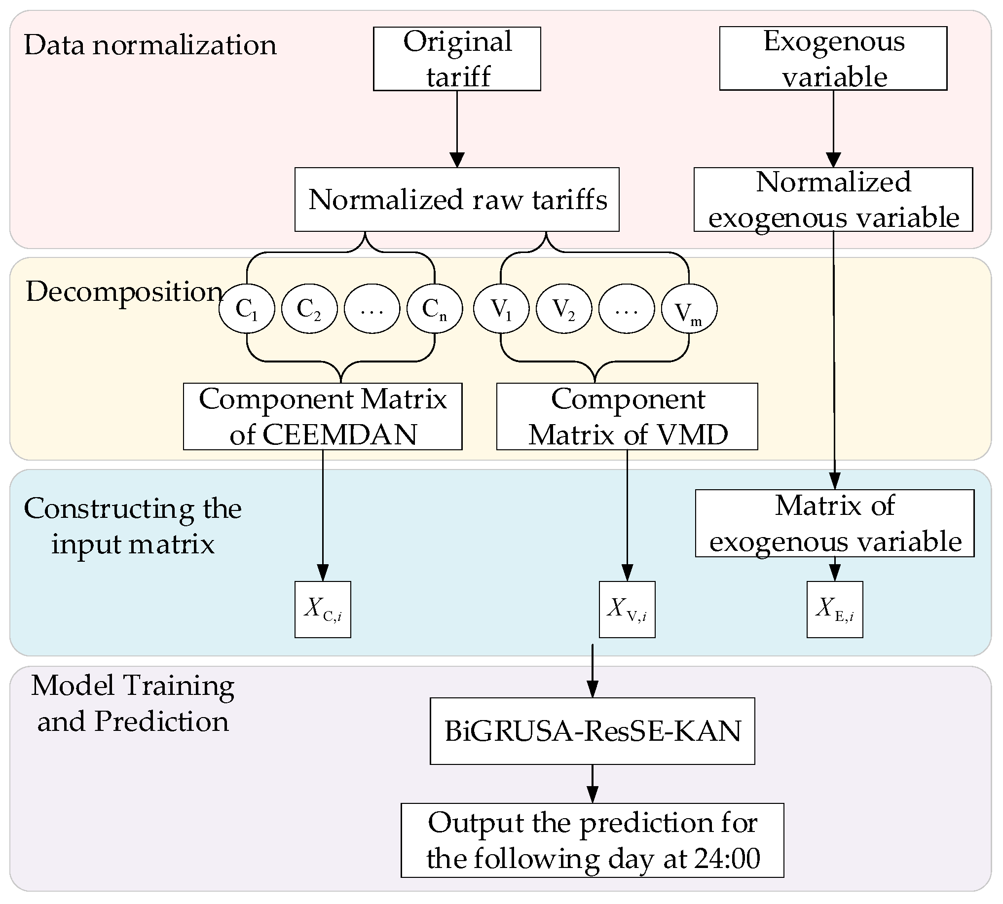
2. Forecasting Process

In this paper, we introduced a basic flow of electricity price prediction based on multi-modal feature fusion and BiGRUSA-ResSE-KAN deep learning model as shown in Figure 1, which mainly includes its main steps as follows:

(1) First, the dataset is normalized. In this paper, the maximum–minimum normalization method is used to map the raw tariffs and exogenous variable data of the five markets to the [−1, 1] interval, in order to eliminate the quantitative differences between the features of the electricity market data and avoid their adverse effects on the model prediction accuracy, so as to improve the training effect and prediction accuracy.

(2) Then, the multi-modal decomposition of the electricity price data was carried out. The CEEMDAN and VMD methods were used to decompose the electricity price data of the five electricity markets respectively, and then, based on the order of frequency from high to low, the components obtained from each method were rearranged and combined, and two multi-scale electricity price component matrices that can reveal the fluctuation law and change trend of electricity price more precisely were finally formed.

(3) Subsequently, the input matrix is constructed. In order to construct the input structure adapted to the time-series features of the deep learning model, this paper ensures the length of the sliding window is consistent with the length of the prediction target (for 24) and divides the CEEMDAN component matrix, the VMD component matrix, and the matrix of the external variables obtained from the five electricity markets, respectively, and obtains the input matrices $X_{\mathrm{C},i}$, $X_{\mathrm{V},i}$, and $X_{\mathrm{E},i}$.

(4) Finally, model training and prediction are performed. $X_{\mathrm{C},i}$, $X_{\mathrm{V},i}$, and $X_{\mathrm{E},i}$ are used as the input matrices of branches 1, 2, and 3, respectively, which are inputted into the BiGRUSA-ResSE-KAN deep learning model for training and prediction, and finally the prediction results of the tariffs of the next day at 24 points are output.

3. Data Preprocessing

3.1. Introduction to the Dataset

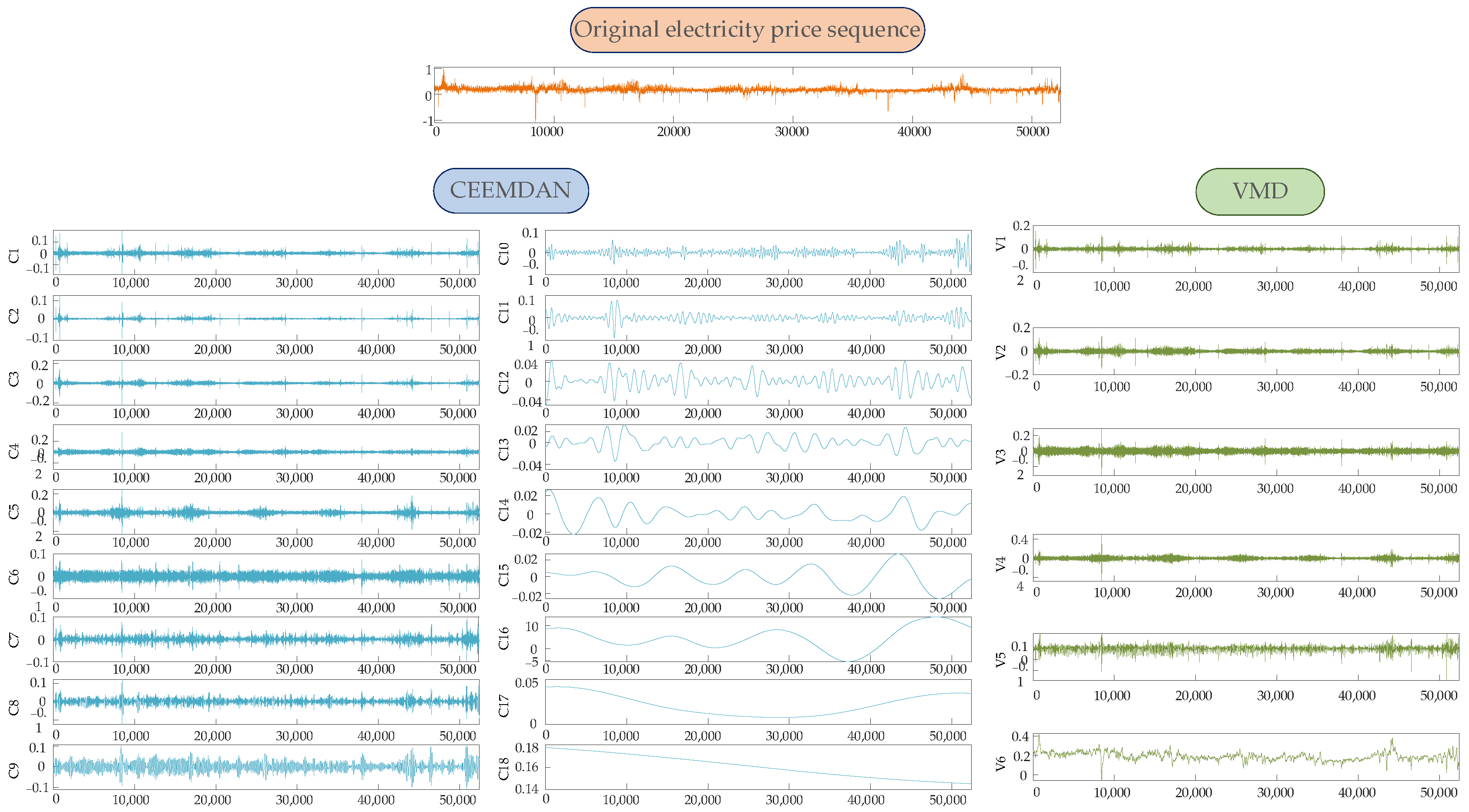
This study evaluates the introduced method’s efficacy in short-term electricity price forecasting, specifically targeting day-ahead predictions. Using an open dataset [20], we analyze five major markets: Northern Europe (NP), the US (PJM), Belgium (EPEX-BE), France (EPEX-FR), and Germany (EPEX-DE). Each provides six years of hourly price data with two exogenous variables. Training set and test set divisions are detailed in

Table 1. Exogenous variables and dataset partitioning corresponding to five power markets.

Electricity Market	Exogenous Variable 1	Exogenous Variable 2	Training Set	Test Set
NP	The day-ahead load forecast	The day-ahead wind generation forecast	1 January 2013–26 December 2016	27 December 2016–24 December 2018
PJM	The day-ahead system load forecast	The day-ahead zonal load forecast	1 January 2013–26 December 2016	27 December 2016–24 December 2018
EPEX-BE	The day-ahead load forecast in France	The day-ahead generation forecast in France	9 January 2011–3 January 2015	4 January 2015–31 December 2016
EPEX-FR	The day-ahead load forecast	The day-ahead generation forecast	9 January 2011–3 January 2015	4 January 2015–31 December 2016
EPEX-DE	The day-ahead zonal load forecast in Amprion	The day-ahead wind generation forecast	9 January 2012–3 January 2016	4 January 2016–31 December 2017

.

Table 1 summarizes the main characteristics of each market. Specifically, the NP electricity market involves electricity trading between the Nordic regions, and its dataset covers hourly observations of day-ahead tariffs, day-ahead load forecasts, and day-ahead wind generation forecasts. The dataset for the PJM electricity market includes day-ahead tariffs for the Commonwealth Edison (COMED) region, a description of the system load, and a two-day-ahead load forecast describing the load in the COMED region. The remaining three markets are from the European Power Exchange (EPEX). The EPEX-BE and the EPEX-FR markets represent the French day-ahead load forecast and the day-ahead generation forecast as exogenous variables, respectively. Finally, the EPEX-DE dataset includes, in addition to day-ahead tariffs, day-ahead zonal load forecasts for the Amprion region of the transmission system operator (TSO), as well as day-ahead wind and solar generation forecasts for the regions of Amprion, TenneT, and 50Hertz (i.e., the three largest TSO regions).

In order to eliminate the dimensional differences among different features of the electricity market data and avoid the adverse effects on the prediction accuracy of the model due to inconsistent feature scales, the maximal–minimum normalization method is adopted to process the data. The core idea of this method is to take the maximum and minimum values of the data as references and map the range of the original data to a unified scale through linear transformation. In particular, this paper chooses to map the data to the interval [−1, 1], aiming to eliminate the influence of dimensional differences on feature weights, thereby improving the training effect and prediction accuracy of the model. The corresponding formula is:

$$X_{\mathrm{norm}}={\displaystyle \frac{2\left(X-X_{\min }\right)}{X_{\max }-X_{\min }}}-1$$

(1)

where $X$ is the original data, $X_{\mathrm{norm}}$ is the normalized data, $X_{\min }$ is the minimum value in the dataset, $X_{\max }$ is the maximum value in the dataset.

3.2. CEEMDAN

CEEMDAN is an enhanced signal decomposition technique developed from EMD and EEMD [21]. This algorithm assists the decomposition process by adding a limited number of adaptive Gaussian white noises to the signal, effectively reducing the reconstruction error, improving the decomposition efficiency, and successfully solving the modal aliasing problem existing in EMD, as well as the problems of high computational complexity and excessive number of inherent modal functions in EEMD.

3.3. VMD

VMD is a completely nonrecursive method for modal variational and signal processing [22]. Its goal is to decompose the historical error data of the transformer into multiple sub-signals with independent center frequencies and sparse features, and it has the ability to handle both recursive and nonrecursive signals simultaneously [23]. The core idea is to construct and solve the variational problem. Compared with EMD and local mean decomposition, it shows better robustness and can better suppress modal aliasing and endpoint effects.

In this study, for the electricity price series of five electricity markets, two signal decomposition algorithms, CEEMDAN and VMD, were respectively adopted for decomposition. During the CEEMDAN decomposition process, the NP market and the EPEX-FR market each obtained 17 sub-components of electricity prices, while the other three markets all generated 18 sub-components of electricity prices. In contrast, during the VMD process, all five markets consistently obtained six sub-components of electricity prices. Taking the DE electricity market as an example, the result of its electricity price decomposition is shown in Figure 2. The figure clearly shows the pronounced differences in the fluctuation characteristics and changing trends of the electricity price components obtained by the two decomposition methods. These electricity price sub-components obtained by different decomposition algorithms are introduced into the deep learning model as input data, aiming to deeply explore the implicit fluctuation patterns and changing trends behind electricity prices. In this way, the effective complementarity of the rules among the sub-components of electricity prices obtained by different decomposition methods was achieved, further enhancing the model’s ability to understand and analyze electricity price data [24].

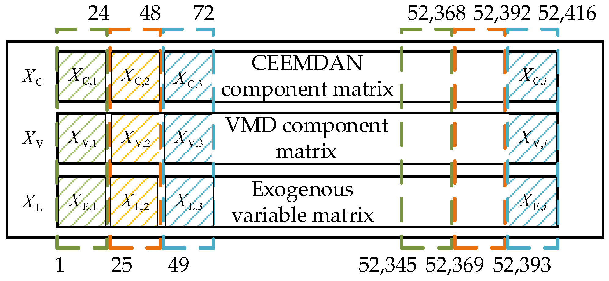
3.4. Construct the Input Matrix

For each electricity price market, three types of input matrices were constructed respectively, including the CEEMDAN decomposition component matrix $X_{\mathrm{C}}$, the VMD component matrix $X_{\mathrm{V}}$, and the exogenous variable matrix $X_{\mathrm{E}}$. In the day-ahead electricity price prediction task, the prediction target usually covers the electricity prices at 24 consecutive time points in the coming day. In order to effectively capture the daily periodic characteristics of the electricity price series, the length of the sliding window is set to be consistent with the length of the predicted target, that is, 24. Taking the DE electricity market as an example, the two multi-scale electricity price component matrices obtained by using the method described in Section 3.3, combined with the external variable matrix composed of two external influencing factors, are sampled according to the sliding window with a length of 24. The input matrices with dimensions of [24,18], [24,6], and [24,2] were obtained respectively as $X_{\mathrm{C},i}$, $X_{\mathrm{V},i}$, and $X_{\mathrm{E},i}$. The specific process of sliding sampling is shown in Figure 3. For the remaining four electricity markets, the same input matrix construction process is adopted. This standardized process ensures the consistency and comparability of all market input data, providing a solid foundation for the subsequent day-ahead electricity price prediction task.

4. Deep Learning Model

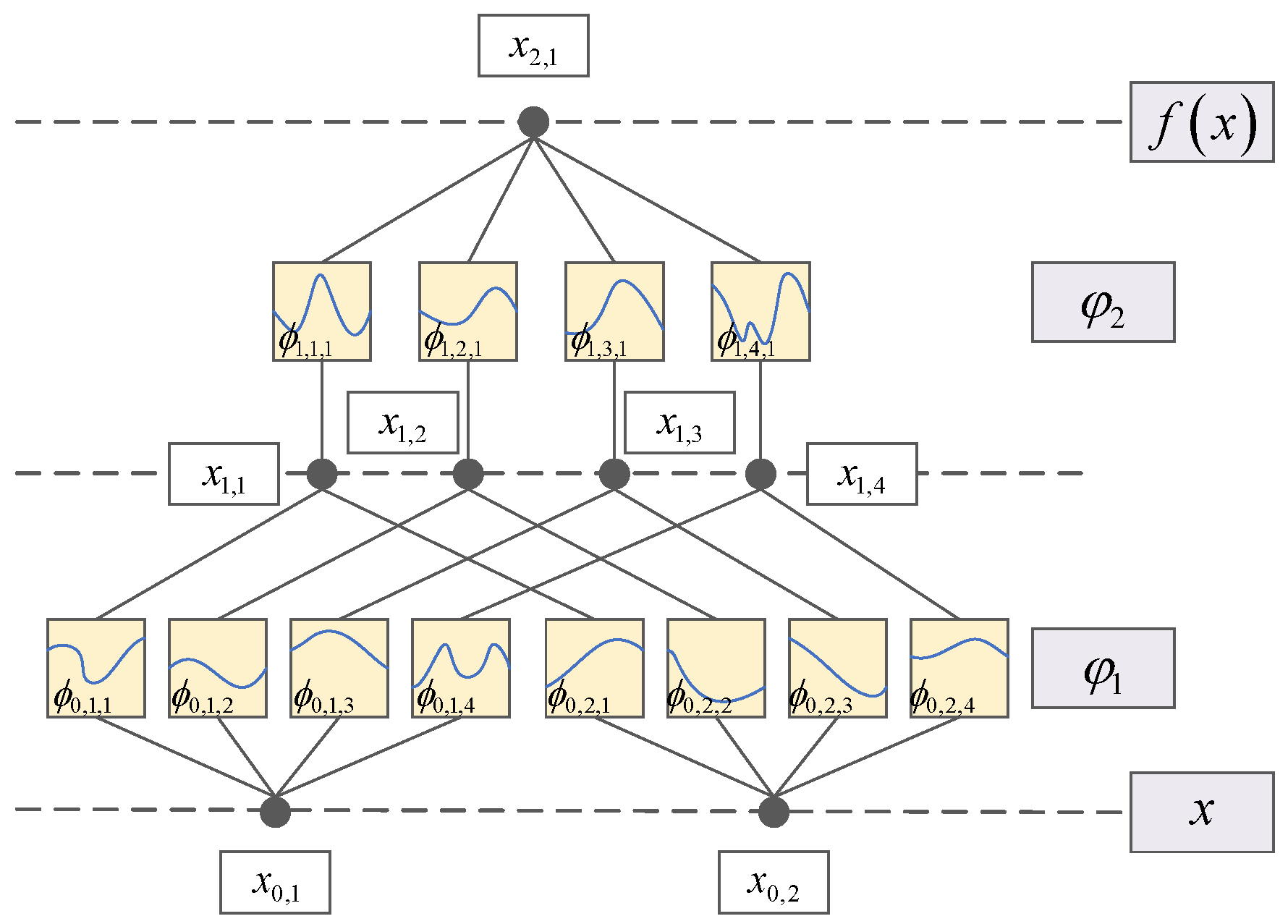
4.1. KAN

KAN, as a new neural network architecture based on the Kolmogorov–Arnold theorem [25], offers a breakthrough in the introduction of learnable edge activation functions. This design concept breaks the traditional mode of multi-layer perceptron (MLP) configuring fixed activation functions at nodes. Instead, it assigns activation functions to the network edges, namely weights, and enables them to have learning capabilities. This transformation not only realizes the independent nonlinear transformation of each coordinate axis but also constructs a multi-dimensional space by combining these transformations, thereby significantly distinguishing it from the layer-by-layer unified nonlinear transformation of MLP in terms of transformation mode. The design advantages of the KAN are prominent. It supports optimization techniques such as network sparsification and pruning, enhancing the interpretability and generalization ability of the model. Meanwhile, this network architecture combines the advantages of spline functions and MLP. It can not only maintain high accuracy in the low-dimensional space but also adapt to the complexity of the high-dimensional space, demonstrating excellent expression ability. Therefore, since its introduction, KANs have demonstrated broad application prospects in traditional fields such as function fitting in mathematical physics and solving partial differential equations, as well as emerging fields such as time-series prediction, graph learning, and computer vision [7]. In these applications, KANs often replace MLP by means of strip function fitting. Especially in the optimized CNN structure, nonlinear activation functions are integrated into the CNN, achieving a smoother parameter representation and thereby improving the accuracy and interpretability of the model. The model formula of the KAN is [26]:

$$f\left(x\right)={\displaystyle \sum _{q=1}^{2n+1}{\phi }_q}\left({\displaystyle \sum _{p=1}^n{\varphi }_{q,p}\left(x_p\right)}\right)$$

(2)

where $f\left(x\right)$ is the output of the function, $2n+1$ is the upper limit of the outer summation, $x_p$ is the pth component of the vector $x$, its range of $1~n$,${\varphi }_{q,p}\left(x_p\right)$ is the internal function, which is the combination of the functions of the qth and pth terms, and ${\phi }_q$ is the external function, which is a function of the qth term of the outer summation.

A KAN layer is a one-dimensional function matrix:

$$\phi =\left\{{\varphi }_{q,p}\right\},p=1,2,\dots n_{in},q=1,2,\dots n_{out}$$

(3)

To build a deep KAN, that is, make a simple stack of each layer of the KAN, the transition matrix of the input and output layers is:

$$x_{l+1}=\left(\begin{array}{cccc}{\varphi }_{l,1,1}(\cdot )& {\varphi }_{l,1,2}(\cdot )& \dots & {\varphi }_{l,1,n_l}(\cdot )\\ {\varphi }_{l,2,1}(\cdot )& {\varphi }_{l,2,2}(\cdot )& \dots & {\varphi }_{l,2,n_l}(\cdot )\\ ⋮& ⋮& \dots & ⋮\\ {\varphi }_{l,n_{l+1},1}(\cdot )& {\varphi }_{l,n_{l+1},2}(\cdot )& \dots & {\varphi }_{l,n_{l+1},n_l}(\cdot )\end{array}\right)x_l$$

(4)

where ${\varphi }_l$ is the matrix function corresponding to the lth KAN layer, ${\varphi }_{l,i,j}$ is the activation function of each edge, that is, the nonlinear transformation. The number of KAN layer nodes is determined by the number of input nodes. Then, the cascading relationship of the multi-layer functions is written in matrix form:

$$\mathrm{KAN}\left(x\right)=\left({\phi }_{L-1}\circ {\phi }_{L-2}\circ \dots \circ {\phi }_1\circ {\phi }_0\right)x$$

(5)

where $\mathrm{KAN}\left(x\right)$ is the output of the KAN, ${\phi }_L$ is the function matrix of the corresponding Lth KAN layer, “$\circ$” is inter-layer connections and functions.

The model architecture of the KAN is shown in Figure 4:

Due to the nonstationarity, complex periodicity, and nonlinearity of electricity price signals, flexible nonlinear methods need to be adopted for modeling. The traditional MLP model struggles to accurately capture the nonlinear changes of signals in different frequency domains because it uses a fixed activation function. The learnable activation function of KANs can be dynamically adjusted to flexibly perceive medium and short-term disturbances, medium fluctuations, and long-term trends in electricity prices. Therefore, in this paper, the KAN is introduced into the traditional deep learning model to provide an accurate and reliable information basis for electricity price prediction and enrich the nonlinear expression ability of the electricity price prediction model.

4.2. BiGRUSA-ResSE-KAN Structure

To improve the prediction accuracy of the day-ahead electricity price in each market, this paper introduced a BiGRUSA-ResSE-KAN deep learning prediction model based on multi-modal feature fusion, and its architecture is shown in Figure 5. This model adopts a three-branch parallel input structure. Each branch takes the CEEMDAN decomposition component matrix, the VMD component matrix, and the exogenous variable matrix as inputs, respectively, forming a joint representation of multi-granularity time-series features and heterogeneous external information. Each branch adopts a sequential–spatial dual-path parallel structure: the sequential path extracts sequence features through the BiGRU module, and the spatial path uses the residual network structure for multi-dimensional variable correlation modeling. The outputs of the two channels are respectively connected to the self-attention mechanism (SA) and the channel attention module (SENet) for feature enhancement. The enhanced features are concatenated and input into the KAN module. High-dimensional nonlinear mapping is achieved through its learning edge function, and finally the prediction results are output by the double-layer fully connected network.

Take Branch 1 as an example. The extraction of temporal path features is implemented by the BiGRU module. Input the feature matrix with the input dimension of $n\times k$ into the BiGRU module to mine the bidirectional temporal rules in the multi-scale electricity price feature matrix and the correlation features among each component and each external variable and obtain the output. Its calculation process is as follows:

$$\left\{\begin{array}{l}{h}_{t,1}=\mathrm{GRU}\left(x_t+h_{t-1,1}\right)\hfill \\ h_{t,2}=\mathrm{GRU}\left(x_t+h_{t-1,2}\right)\hfill \\ f_1^1={\alpha }_t{h}_{t,1}+{\beta }_t{h}_{t,2}+b_t\hfill \end{array}\right.$$

(6)

where $\mathrm{GRU}\left(·\right)$ represents the gated loop unit, $h_{t,1}$ and $h_{t,2}$ are the outputs of the hidden layers in the forward and backward directions, respectively, $h_{t-1,1}$ indicate the hidden state of the forward hidden state at the previous moment, $h_{t-1,2}$ is the hidden state of the backward hidden state at the next moment, ${\alpha }_t$, ${\beta }_t$ represent respectively the weights corresponding to the forward hidden layer state and the reverse hidden layer state corresponding to BiGRU at the moment t, $b_t$ is the bias value corresponding to the state of the hidden layer at the moment t, $f_1^1$ is the output of the BiGRU module.

The feature extraction of spatial paths is achieved by using the residual network module. This module contains two parallel convolutional paths, which are respectively configured with convolutional kernels of different scales (3 × 3 and 5 × 5). Through multi-scale convolutional operations, the local and global spatial correlations of the input matrix are captured, achieving multi-receptive field feature fusion and effectively extracting the hierarchical spatial dependencies among multi-dimensional variables. Its calculation process is as follows:

$$\left\{\begin{array}{l}{f}_{1,1}^2=\delta ({\displaystyle \sum {\omega }_{1,1}^i}\ast X_{\mathrm{p}}+{\lambda }_{1,1}^i)\\ f_{1,2}^2=\delta ({\displaystyle \sum {\omega }_{1,2}^i}\ast f_{1,1}^2+{\lambda }_{1,2}^i)\\ f_{2,1}^2=\delta ({\displaystyle \sum {\omega }_{2,1}^i}\ast X_{\mathrm{p}}+{\lambda }_{2,1}^i)\\ f_R^2=F_{\mathrm{L}}(f_{1,2}^2+f_{2,1}^2)\end{array}\right.$$

(7)

where $X_{\mathrm{p}}$ is the model input, “$\ast$” is the convolution operation, $f_{1,1}^2$ and $f_{1,2}^2$ are the first layer convolution and second layer convolution output feature of convolution block 1, $f_{2,1}^2$ is the output feature of convolutional block 2, ${\omega }_{1,1}^i$, ${\omega }_{1,2}^i$, ${\omega }_{2,1}^i$ and ${\lambda }_{1,1}^i$, ${\lambda }_{1,2}^i$, ${\lambda }_{2,1}^i$ are the weight matrices and bias parameters of the first filter of convolutional block 1 and convolutional block 2, $\delta \left(·\right)$ is the activation function of ReLU, $F_{\mathrm{L}}$ is the flatten function, $f_R^2$ is the output of the residual module.

The tensor slicing operation is performed on the output features of the three-branch BiGRU module to extract the last time-step feature of each sample. The time-series features $f_{B,C}$, $f_{B,V}$, and $f_{B,E}$ extracted by each of the three branches are concatenated and fused into $f_B$ and then input into the SA module. The long-range dependency across time steps is constructed through its global receptive field to achieve the adaptive focusing of key information in the feature space, thereby enhancing the discriminative expression ability of temporal series features. The calculation process is as follows:

$$f_{\mathrm{B}}=f_{\mathrm{B},\mathrm{C}}\oplus f_{\mathrm{B},\mathrm{V}}\oplus f_{\mathrm{B},\mathrm{E}}$$

(8)

$$\left\{\begin{array}{l}Q=f_{\mathrm{B}}\times W_q\\ K=f_{\mathrm{B}}\times W_k\\ V=f_{\mathrm{B}}\times W_v\\ f_B^A=\mathrm{softmax}({\displaystyle \frac{Q\times K^T}{\sqrt{d_k}}})\end{array}\right.$$

(9)

where “⊕” is the stacking processing of the features obtained from each branch, $f_{\mathrm{B}}$ is a one-dimensional long vector obtained by stacking and fusing the features of three branches. $W_q$, $W_k$, and $W_v$ are the query, key, and value weight matrix corresponding to the SA module, $Q$, $K$, and $V$ are the query, key, and value matrix corresponding to the SA module, $\mathrm{softmax}$ is a normalized function, $T$ is a matrix transposition operation, $d_k$ is the normalized parameter, $f_B^A$ is the feature sequence output by the SA module.

The features extracted from the three-branch residual part are combined into $f_R$ and input into SENet. The correlation relationship is constructed for the feature channels of the residual part, the correlation information between channels is learned, the weight information of each feature channel is obtained, the feature channels carrying important information are enhanced, the feature channels carrying redundant information are suppressed, and the performance of the residual module is improved. Its calculation process is as follows:

$$f_R=Conca{t}_3(f_{R,C},f_{R,V},f_{R,E})$$

(10)

where $f_{R,C}$, $f_{R,V}$, and $f_{R,E}$ are the outputs of the residual parts of branches 1, 2, and 3, respectively. The combined output of the three is $f_R$. $Conca{t}_3$ is the merging operation of the 3D tensor $f_{R,i}\in R^{W\times H\times C}$ in the C channel dimension.

$$\left\{\begin{array}{l}z={\mathrm{F}}_{sq}(f_R)={\displaystyle \frac{1}{W\times H}}{\displaystyle \sum _{i=1}^W{\displaystyle \sum _{j=1}^H{f}_R(i,j)}}\\ s={\mathrm{F}}_{ex}(z,W)=\sigma (g(z,W))=\sigma (W_2\delta (W_{1}z))\\ s=[s_1,\cdot \cdot \cdot ,s_n,\cdot \cdot \cdot ,s_N]\\ {\tilde{x}}_n={\mathrm{F}}_{scale}(f_{R,n},s_n)=f_{R,n}\cdot s_n\\ f_R^A=\tilde{X}=[{\tilde{x}}_1,\cdot \cdot \cdot ,{\tilde{x}}_n,\cdot \cdot \cdot ,{\tilde{x}}_N]\end{array}\right.$$

(11)

where $W$, $H$, $C$ are respectively the batch, the length of the electricity price sequence, and the number of channels. The three-dimensional features are compressed into a $1\times 1$ feature factor to represent the feature information of the feature channel. For $C$ feature channels, the feature vector $1\times 1\times C$ of $z$ is obtained, thereby enabling the network to obtain the global receptive field. $\delta \left(·\right)$ is the activation function of ReLU, $\sigma \left(·\right)$ is the sigmoid activation function, $W_1\in R^{(C/r)\times C}$ and $W_2\in R^{(C/r)\times C}$ are the parameters of the two fully connected layers, $f_{R,n}$ is the matrix of the nth channel of $f_R$, $s_n$ is the weight of the $n$th channel of the weight vector $s$, ${\mathrm{F}}_{scale}(·,·)$ is the multiplication of channel dimensions, $f_R^A$ is the feature sequence output by the residual module.

Merge the features $f_B^A$ and $f_R^A$ extracted by the two groups of attention mechanisms and input them into the KAN module. Its calculation formula is:

$$\left\{\begin{array}{l}F=Concat(f_B^A,f_R^A)\\ F_K=\left({\phi }_{L-1}\circ {\phi }_{L-2}\circ \dots \circ {\phi }_1\circ {\phi }_0\right)F\end{array}\right.$$

(12)

where the combined output of the feature $f_B^A$ extracted by the SA module and the feature $f_R^A$ extracted by the SENet module is $F$. $F_K$ represents the output of the KAN, ${\phi }_L$ is the function matrix corresponding to the Lth KAN layer, “$\circ$” is the symbol of inter-layer connections and functions.

Finally, the predicted output $Y$ is obtained by adding nonlinear expressions through two fully connected layers. Its calculation formula is:

$$\left\{\begin{array}{l}{F}_C=\delta (W_C{F}_K+b_c)\\ Y=\delta (W{F}_C+b)\end{array}\right.$$

(13)

where $W_C$, $W$ and $b_c$, $b$ are the weight matrices and bias parameters of the two fully connected layers.

5. Experimental Verification

5.1. Platform and Model Configuration

The hardware environment for the experiment operation includes CPU (Intel Core i5-12600KF 3.6 GHz), RAM (DDR4 32 GB), and GPU (NVIDIA GeForce RTX 3060 12 G). The programming language adopted is Python 3.12.4, and the construction of the deep learning model is carried out in the environments of PyTorch 1.10.1, CUDA 11.3, and PyCharm 2024.1. Furthermore, the CEEMDAN decomposition and VMD tasks are performed using MATLAB 2023b. During the training process, Adam was selected as the optimization algorithm, with its learning rate set at 0.0001 and the maximum number of iterations being 1000 times. In terms of batch size, it is set at 28 for the NP and DE markets, and 8 for the PJM, BE, and FR markets. To reduce the random errors and accidental factors in the experiments, this paper adopts the strategy of averaging the experiments. Specifically, each group of experiments is independently repeated 10 times, and the arithmetic mean of the results of these 10 experiments is taken as the final prediction result to ensure the stability and credibility of the experimental results. The division of the training set and test set of each market electricity price is shown in Table 1.

5.2. Evaluation Index

In the field of electricity price prediction, in order to realize an objective evaluation of the experimental results and to ensure the comparability of the research results with the existing literature, this paper selects five widely used evaluation indexes: mean absolute error (MAE), mean absolute percentage error (MAPE), symmetric mean absolute percentage error (sMAPE), root mean squared error (RMSE), and coefficient of determination (R²). These metrics quantify the degree of deviation between the predicted value and the true value through de-signification. Their calculation formulas are as follows:

$$\mathrm{MAE}={\displaystyle \frac{1}{24N_{\mathrm{d}}}}{\displaystyle \sum _{d=1}^{N_{\mathrm{d}}}{\displaystyle \sum _{h=1}^{24}|{\widehat{P}}_{d,h}-P_{d,h}|}}$$

(14)

$$\mathrm{MAPE}={\displaystyle \frac{1}{24N_{\mathrm{d}}}}{\displaystyle \sum _{d=1}^{N_{\mathrm{d}}}{\displaystyle \sum _{h=1}^{24}\frac{|{\widehat{P}}_{d,h}-P_{d,h}|}{\left|P_{d,h}\right|}}}\times \mathrm{100\%}$$

(15)

$$\mathrm{sMAPE}={\displaystyle \frac{1}{24N_{\mathrm{d}}}}{\displaystyle \sum _{d=1}^{N_{\mathrm{d}}}{\displaystyle \sum _{h=1}^{24}2\frac{|{\widehat{P}}_{d,h}-P_{d,h}|}{\left|{\widehat{P}}_{d,h}\right|+\left|P_{d,h}\right|}}}\times \mathrm{100\%}$$

(16)

$$\mathrm{RMSE}=\sqrt{{\displaystyle \frac{1}{24N_{\mathrm{d}}}}{\displaystyle \sum _{d=1}^{N_{\mathrm{d}}}{\displaystyle \sum _{h=1}^{24}{\left({\widehat{P}}_{d,h}-P_{d,h}\right)}^2}}}$$

(17)

$$R^2=1-{\displaystyle \frac{\frac{1}{24N_{\mathrm{d}}}{\displaystyle \sum _{d=1}^{N_{\mathrm{d}}}{\displaystyle \sum _{h=1}^{24}{({\widehat{P}}_{d,h}-P_{d,h})}^2}}}{\frac{1}{24N_{\mathrm{d}}}{\displaystyle \sum _{d=1}^{N_{\mathrm{d}}}{\displaystyle \sum _{h=1}^{24}{({\overline{P}}_d-P_{d,h})}^2}}}}$$

(18)

where $N_{\mathrm{d}}$ is the number of test days for the test set, $d$ is a certain day in the test set, $h$ is a certain hour on a certain day in the test set, $P_{d,h}$ is the true value of the test electricity price data. ${\widehat{P}}_{d,h}$ is the predicted value of the test tariff data; ${\overline{P}}_d$ is the average value of the real tariff on the prediction day.

In the prediction and evaluation of electricity prices, MAE is particularly useful when prediction errors linearly affect costs and risks due to its intuitiveness and ease of understanding. However, it is difficult to compare directly among different datasets. Although RMSE is often used in the evaluation of regression models, it has poor interpretability in linearly dependent scenarios such as electricity costs because it is based on quadratic errors. MAPE may distort when the price is close to zero, while sMAPE, as its improved version, reduces the error amplification effect when the market electricity price is close to zero. Although these indicators each have their own characteristics and jointly provide diversified perspectives for prediction and evaluation, they are all greatly influenced by the selected test segment datasets, making it difficult to objectively compare the prediction accuracy among different datasets.

To solve the above problems, the relative mean absolute error (rMAE) is used to evaluate the accuracy of electricity price prediction among different datasets [20]. It is characterized by standardizing the error into relative form, which facilitates the comparison of errors among different datasets or models, effectively solves the influence of different electricity price datasets on the evaluation results, and improves the interpretability of the evaluation results. Its calculation formula is as follows:

$$\mathrm{rMAE}={\displaystyle \frac{\frac{1}{24N_{\mathrm{d}}}{\displaystyle \sum _{d=1}^{N_{\mathrm{d}}}{\displaystyle \sum _{h=1}^{24}|{\widehat{P}}_{d,h}-P_{d,h}|}}}{\frac{1}{24N_{\mathrm{d}}}{\displaystyle \sum _{d=1}^{N_{\mathrm{d}}}{\displaystyle \sum _{h=1}^{24}|{\widehat{P}}_{d-7,h}-P_{d,h}|}}}}$$

(19)

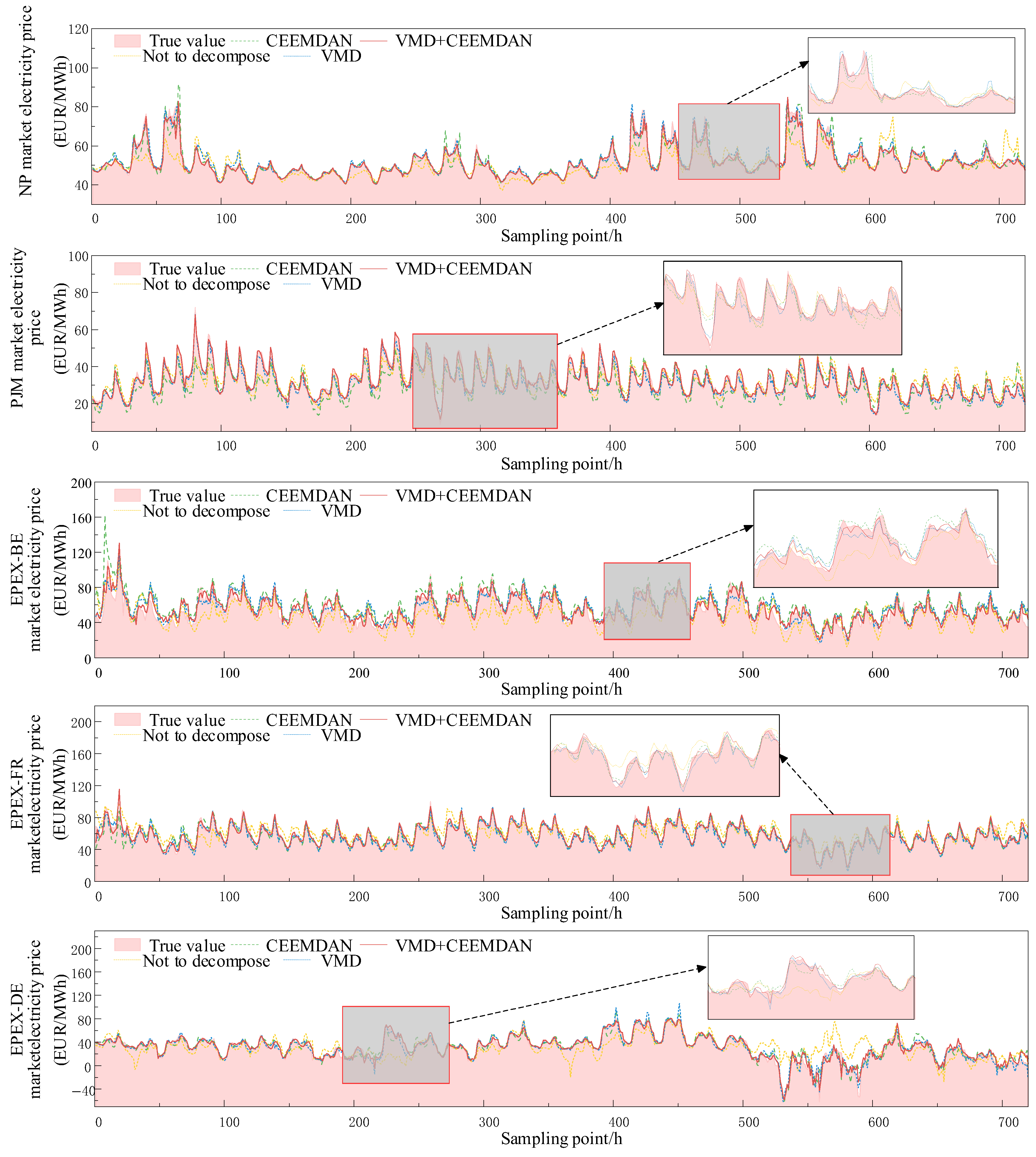
5.3. Verification Experiment of the Validity of Double Decomposition Input Matrix

In order to verify the superiority of the hybrid mode decomposition, this paper respectively builds the original data input matrix and the BiGRUSA-ResSE-KAN electricity price prediction model based on the single-mode decomposition of CEEMDAN and VMD and compares them with the models under the hybrid mode decomposition. For the convenience of observation, the data of the last 30 days of each electricity market are selected to draw the prediction curve for comparison. As shown in Figure 6, the evaluation indicators predicted by different decomposition schemes are presented in

Table 2. Prediction error of different decomposition schemes in each power market.

Dataset	Metric	Original Data	CEEMDAN	VMD	VMD + CEEMDAN
NP	rMAE	0.587	0.269	0.193	0.173
	MAE	2.429	1.111	0.798	0.732
	MAPE (%)	6.978	3.121	2.239	2.067
	sMAPE (%)	6.732	3.175	2.282	2.082
	RMSE	4.268	2.296	1.539	1.438
	R2	0.841	0.954	0.979	0.980
PJM	rMAE	0.822	0.677	0.332	0.194
	MAE	5.201	4.280	2.102	1.224
	MAPE (%)	15.819	17.587	10.318	5.934
	sMAPE (%)	17.773	16.196	8.877	5.212
	RMSE	9.405	8.214	2.934	1.736
	R2	0.496	0.563	0.932	0.970
EPEX-BE	rMAE	0.873	0.831	0.707	0.466
	MAE	8.866	8.445	7.186	4.730
	MAPE (%)	27.027	19.957	16.112	12.213
	sMAPE (%)	22.696	20.312	17.518	12.066
	RMSE	18.169	15.391	13.825	11.116
	R2	0.461	0.549	0.636	0.684
EPEX-FR	rMAE	1.203	0.534	0.435	0.373
	MAE	8.822	3.916	3.191	2.736
	MAPE (%)	20.242	13.223	11.524	9.333
	sMAPE (%)	23.256	10.848	9.509	7.415
	RMSE	15.414	14.997	9.911	10.264
	R2	0.483	0.516	0.713	0.726
EPEX-DE	rMAE	0.835	0.353	0.233	0.232
	MAE	7.621	3.222	2.128	2.113
	MAPE (%)	49.166	18.368	13.622	11.350
	sMAPE (%)	28.069	12.783	9.411	9.235
	RMSE	12.394	5.660	4.178	4.141
	R2	0.639	0.866	0.926	0.929

.

An analysis of Table 2 shows that, when no decomposition methods are adopted, the prediction errors are generally high, especially in indicators such as MAE, MAPE, sMAPE, and RMSE, highlighting the negative impact of the complexity and nonlinear characteristics of the original time-series data on the prediction accuracy. In contrast, the CEEMDAN method effectively reduces the prediction error and shows strong adaptability to complex nonlinear time-series data. The VMD method performs even better. Its unique advantage of decomposing the frequency components improves the prediction accuracy. Compared with the undecomposed data, the MAE of VMD and CEEMDAN decomposition methods decreased by 1.317 and 1.631, 0.921 and 3.099, 0.421 and 1.680, 4.906 and 5.631, and 4.398 and 5.492, respectively. Therefore, for the electricity price sequence processed by decomposition methods and then input into the deep learning model, it can effectively separate features such as trends, cycles, and random fluctuations, enabling the model to capture the multi-scale characteristics of electricity price fluctuations more clearly. At the same time, it reduces noise interference, lowers the training difficulty, enhances the generalization ability, and provides a more structured and information-rich input for the deep learning model, significantly improving the performance and interpretability of the model.

Compared with the single-decomposition mode, the hybrid decomposition combination method of VMD and CEEMDAN has achieved the best prediction performance in all electricity markets. The values of each evaluation index are significantly lower than those of other methods. The rMAE of each market is as low as 0.173, 0.194, 0.466, 0.373, and 0.232, respectively. It indicates that this combined method can extract and utilize the information in time-series data more effectively. Through the principle of complementary decomposition, it improves the accuracy and stability of prediction.

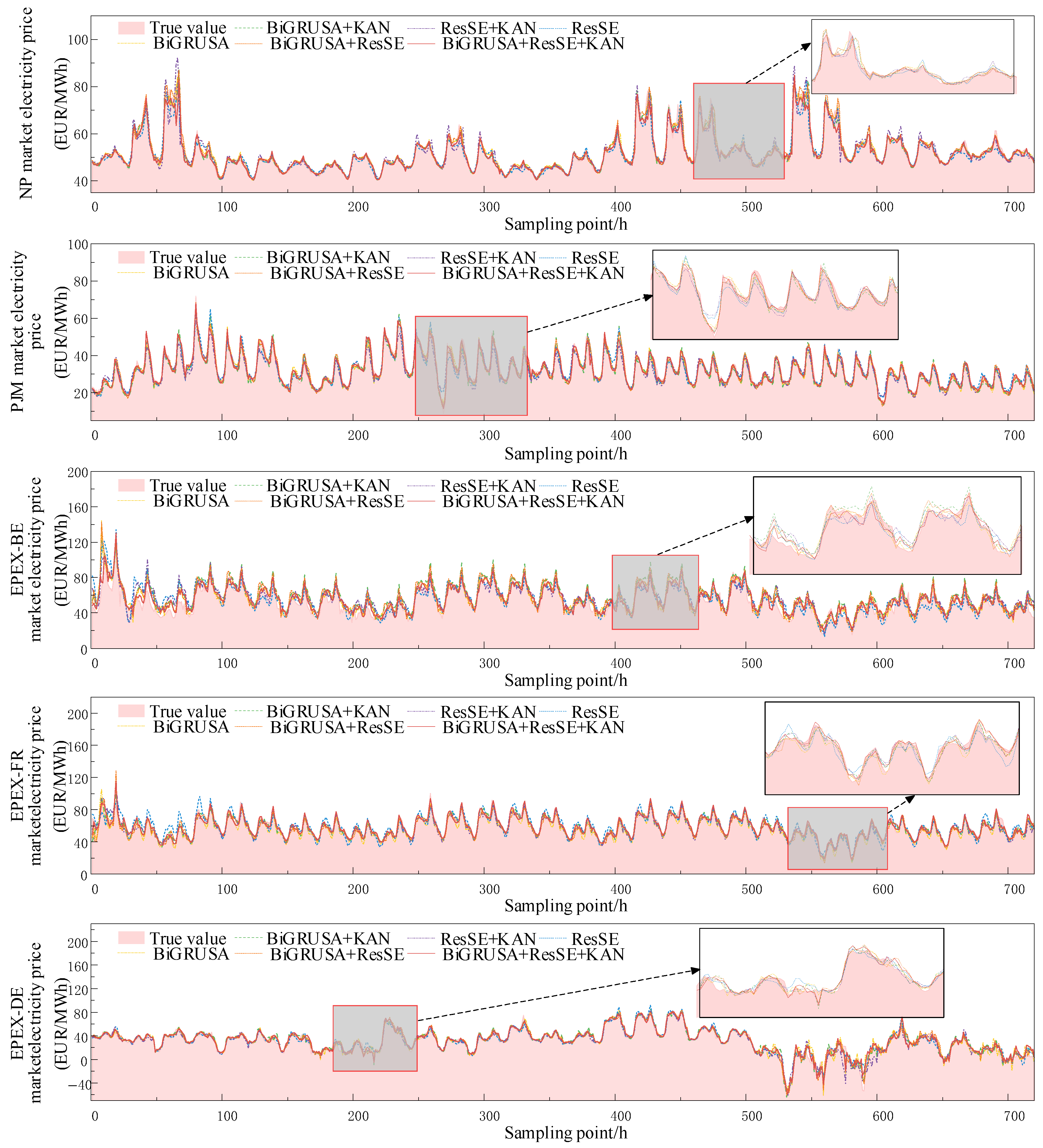
5.4. Ablation Experiment

In order to evaluate and understand the key roles of each module in the deep model and its contribution to the overall performance, an ablation experiment strategy was implemented, aiming to explore and determine the optimal model structure configuration, thereby improving the performance and efficiency of the model. At the same time, the interpretability of the BiGRUSA-ResSE-KAN model was also enhanced. All ablation experiments were trained based on the three-channel input model framework. For the convenience of observation, the data of the last 30 days of each electricity market were selected to draw the prediction curve for comparison, as shown in Figure 7, and the prediction errors are shown in

Table 3. Prediction error of each power market ablation experiment.

Dataset	Metric	BiGRUSA	BiGRUSA-KAN	ResSE	ResSE + KAN	BiGRUSA-ResSE	BiGRUSA-ResSE-KAN
NP	rMAE	0.180	0.173	0.294	0.271	0.180	0.173
	MAE	0.746	0.715	1.216	1.119	0.745	0.732
	MAPE (%)	2.125	2.098	3.485	3.192	2.099	2.067
	sMAPE (%)	2.174	2.094	3.502	3.283	2.153	2.082
	RMSE	1.424	1.449	2.142	1.963	1.459	1.438
	R2	0.979	0.980	0.960	0.967	0.979	0.980
PJM	rMAE	0.275	0.282	0.362	0.356	0.267	0.194
	MAE	1.739	1.784	2.292	2.252	1.686	1.224
	MAPE (%)	8.132	7.968	10.450	9.435	7.569	5.934
	sMAPE (%)	7.148	7.271	9.574	9.551	6.893	5.212
	RMSE	2.770	2.708	3.530	3.387	2.696	1.736
	R2	0.939	0.942	0.901	0.901	0.909	0.970
EPEX-BE	rMAE	0.536	0.672	0.749	0.653	0.598	0.466
	MAE	5.445	6.823	7.609	6.631	6.072	4.730
	MAPE (%)	14.911	15.223	17.018	15.495	13.467	12.213
	sMAPE (%)	12.969	16.059	18.438	15.707	14.210	12.066
	RMSE	14.102	13.456	13.831	13.044	14.117	11.116
	R2	0.621	0.655	0.635	0.676	0.620	0.684
EPEX-FR	rMAE	0.482	0.438	0.838	0.524	0.446	0.373
	MAE	3.531	3.213	6.143	3.841	3.272	2.736
	MAPE (%)	13.848	13.102	17.963	11.781	12.411	9.333
	sMAPE (%)	10.107	8.696	17.806	11.085	9.401	7.415
	RMSE	12.104	12.184	13.711	10.993	10.354	10.264
	R2	0.619	0.614	0.512	0.686	0.721	0.726
EPEX-DE	rMAE	0.236	0.249	0.276	0.259	0.248	0.232
	MAE	2.155	2.273	2.515	2.364	2.264	2.113
	MAPE(%)	18.892	13.515	22.554	18.581	13.213	11.350
	sMAPE(%)	9.290	9.482	10.676	10.289	9.666	9.235
	RMSE	3.905	4.438	4.394	4.652	4.326	4.141
	R2	0.926	0.917	0.919	0.910	0.921	0.929

.

The experimental results in Table 3 show that, compared with other model configurations, BiGRUSA-ResSE-KAN significantly reduces the prediction error in most cases, verifies the rationality of its design, and demonstrates pronounced advantages in different electricity market prediction tasks. Specifically, in the comparison between BiGRUSA and ResSE, using BiGRUSA alone usually shows a lower prediction error. This indicates that the extraction of time-series features may be more important in the prediction of electricity prices, because electricity prices have pronounced time series characteristics, such as seasonality and periodicity. BiGRUSA effectively extracted these temporal features through the bidirectional gated loop unit module, thereby demonstrating an advantage in prediction. However, spatial feature modeling also plays a supplementary role in the prediction of electricity prices. ResSE uses the residual network structure for multi-dimensional variable correlation modeling. Although its prediction performance is not as good as that of BiGRUSA when used alone, when it is added as supplementary information to the model, namely BigRUSA, the prediction performance can be further improved. Among the five electricity price markets, compared with the BiGRUSA model, The BiGRUSA-ResSE model decreased by 0.026%, 0.564%, 1.444%, 1.437%, and 5.679%, respectively, in the MAPE evaluation index. This indicates that the electricity price is not only affected by temporal factors but also jointly influenced by multi-dimensional spatial variables such as power generation and load demand.

In addition, feature enhancement and high-dimensional nonlinear mapping are also key factors for improving the predictive performance of the model. The SA and the SENet enhance the features, enabling the model to focus more on the important feature information. The KAN module realizes high-dimensional nonlinear mapping through learnable edge functions, further enhancing the predictive ability of the model. It is a necessary component in most markets, contributing to an error reduction of more than 10%. The addition of these modules enables the BiGRUSA-ResSE-KAN model to fuse and utilize various feature information more effectively, thereby demonstrating the optimal prediction performance.

Figure 8 presents the prediction effect of the BiGRUSA-ResSE-KAN model on the electricity prices of five markets through a scatter plot. Analysis shows that this model demonstrates excellent long-term spatiotemporal prediction ability within the conventional price range, and the predicted values are highly consistent with the true value distribution. However, in extreme price scenarios, such as sudden peak electricity prices and negative electricity prices, the prediction accuracy fluctuates significantly, highlighting that the model’s ability to capture unconventional price fluctuation patterns still needs to be improved. Further exploration of the model feature extraction mechanism reveals that although its architecture can effectively model the global spatiotemporal dependence of the electricity price sequence, it has limitations in the refined representation of local abnormal features. In response to this limitation, future studies can explore the introduction of multi-scale feature fusion strategies or the construction of anomaly detection modules to enhance the model’s adaptability to nonlinear price dynamics and sudden change features, thereby improving the prediction robustness under extreme market conditions.

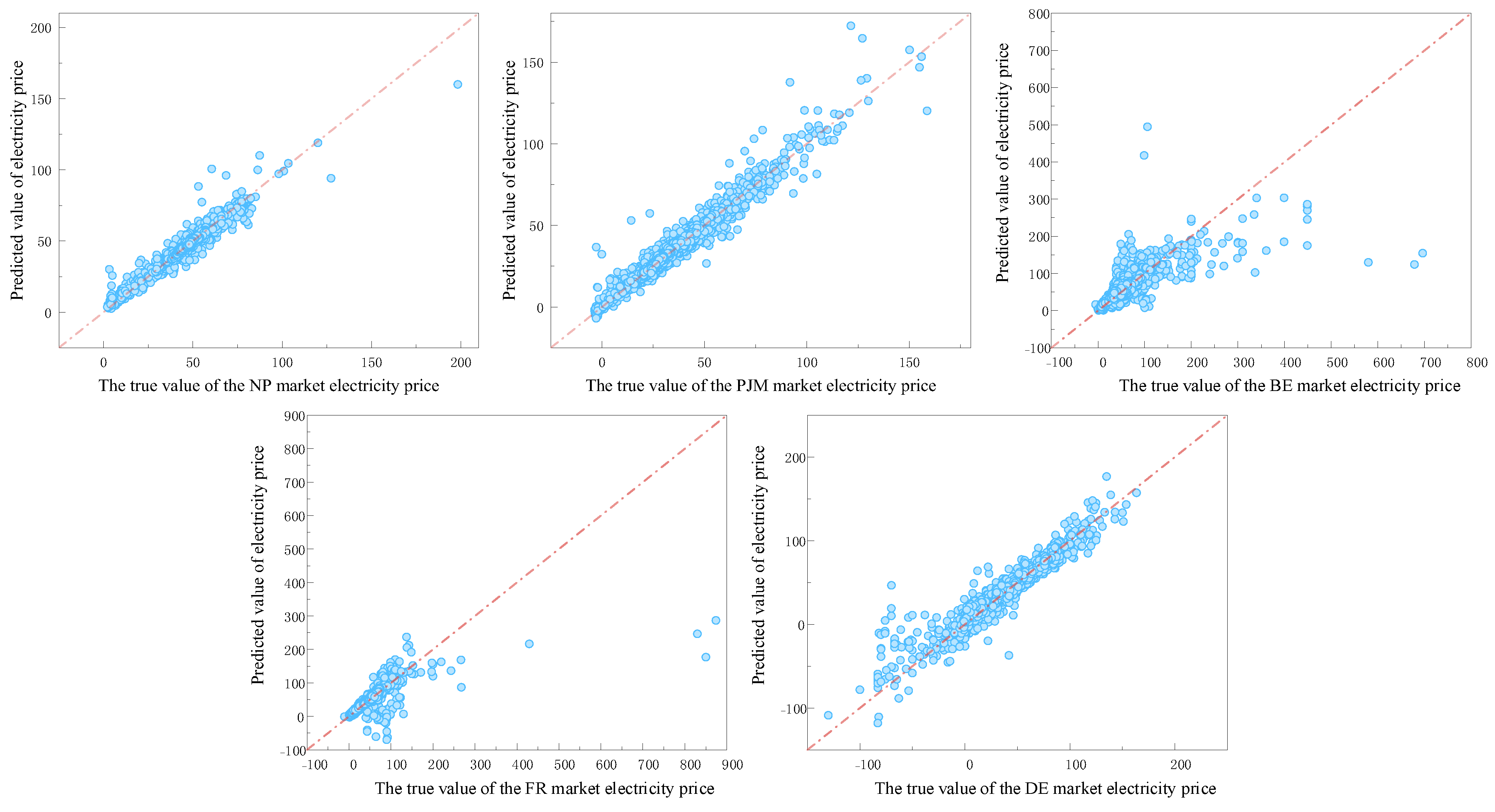
5.5. Comparison of Methods in Different Studies

This paper compares and analyzes a variety of advanced models and methods in current research, including the combination of multiple deep learning architectures, among which there are RNN, CNN, LSTM, and GRU combined with Monte Carlo dropout technology and layer constraints [27], as well as the integration of LEAR and DNN methods [20]. The improved time-series prediction model NBEATSx adopts the methods of introducing exogenous variable processing and multi-source information fusion [28], as well as HeTCN through dual temporal modeling, heteroskedastic uncertainty quantification, dynamic fusion of multi-view features, and variance-aware regularization [29]. The comparison results are detailed in

Table 4. Comparison of different methods of literature under different signal-to-noise ratios.

Dataset	Metric	RNN	CNN	LSTM	GRU	LEAR Ensemble	DNN Ensemble	NBEATSx	HeTCN	BiGRUSA-ResSE-KAN
NP	rMAE	1.220	0.490	1.200	0.400	0.420	0.400	0.530	-	0.173
	MAE	7.300	2.020	7.180	2.410	1.740	1.670	1.680	2.040	0.732
	MAPE (%)	20.190	6.790	19.690	7.760	5.530	5.380	-	-	2.067
	sMAPE (%)	21.500	5.840	21.040	6.840	5.010	4.850	4.890	5.890	2.082
	RMSE	8.360	3.850	8.240	4.240	3.360	3.330	3.330	3.690	1.438
PJM	rMAE	0.520	0.540	0.630	0.420	0.480	0.440	0.620	-	0.194
	MAE	4.140	3.420	4.970	3.370	3.010	2.780	3.010	3.060	1.224
	MAPE (%)	33.040	34.950	45.550	30.750	30.130	28.660	-	-	5.934
	sMAPE (%)	15.880	13.240	19.460	12.970	11.980	11.220	11.910	11.960	5.212
	RMSE	6.370	5.700	6.740	34.940	5.130	4.640	5.000	5.420	1.736
EPEX-BE	rMAE	0.590	0.490	0.580	0.510	0.600	0.570	0.750	-	0.466
	MAE	8.090	6.680	7.880	7.030	6.140	5.820	6.170	6.340	4.730
	MAPE (%)	30.910	30.560	33.790	32.340	20.720	26.110	-	-	12.213
	sMAPE (%)	19.370	16.690	19.210	16.100	14.550	13.330	14.520	15.130	12.066
	RMSE	18.000	15.050	17.800	16.790	15.970	16.130	15.430	16.410	11.116
EPEX-FR	rMAE	0.510	0.430	0.510	0.440	0.540	0.530	0.670	-	0.373
	MAE	5.740	4.860	5.750	4.970	3.980	3.910	3.970	4.350	2.736
	MAPE (%)	17.310	18.430	17.560	18.650	14.680	14.770	-	-	9.333
	sMAPE (%)	16.300	13.410	16.800	14.110	11.570	10.980	11.290	12.770	7.415
	RMSE	13.160	12.420	13.190	12.540	10.680	11.740	11.080	12.020	10.264
EPEX-DE	rMAE	0.520	0.430	0.430	0.430	0.400	0.380	0.420	-	0.232
	MAE	6.010	4.960	4.960	4.990	3.610	3.440	3.370	4.420	2.113
	MAPE (%)	104.560	117.860	109.270	67.140	113.980	95.760	-	-	11.350
	sMAPE (%)	22.590	18.400	18.620	18.540	14.740	14.190	14.340	17.270	9.235
	RMSE	8.870	8.100	7.840	8.190	6.510	6.000	5.640	7.330	4.141

.

In the prediction and comparison experiments of different methods, the method introduced in this paper shows pronounced performance advantages compared with traditional deep learning models and emerging methods. By comparing the five error indicators of rMAE, MAE, MAPE, sMAPE, and RMSE, it is found that the method introduced in this paper achieves the lowest error value in all evaluated markets. Especially in the NP, PJM, and EPEX-DE markets, the decline of the model in this paper in the three key indicators of rMAE, MAE, and MAPE is particularly significant, all exceeding 50%. The MAPE indicators of traditional models such as RNN and LSTM are generally higher than 20% in most markets. Although emerging LEAR Ensemble, DNN Ensemble, NBEATSx, and HeTCN have improved in error performance compared with traditional methods, in complex markets such as EPEX-DE, the MAPE of integration methods deteriorates significantly, showing the limitations of their generalization ability.

Further analysis shows that the data characteristics of different markets have a substantial impact on the model performance. In the low- and medium-complexity tariff markets, such as the NP market and PJM market, the prediction performance of all models performs well, but the model in this paper reduces the error by more than 56% compared to other methods. In markets with high noise and many spiky impulses, such as the EPEX-BE and EPEX-FR markets, the MAPE of the traditional models exceeds 30% and 17%, respectively, while the model in this paper effectively reduces the MAPE to 12.21% and 9.33%. For the EPEX-DE market, which exhibits strong nonlinear and chaotic characteristics, the MAPE evaluation metrics of most models are worse than 95%, whereas this paper’s method significantly reduces the MAPE from 117.86% to 11.35% by the bidirectional feature extraction capability of BiGRU. The experimental results further verify that the hybrid model in this paper is able to adapt itself to the noise levels and volatility patterns of different markets by incorporating multi-module features, thus significantly improving the prediction accuracy.

6. Conclusions

This study introduced a BiGRUSA-ResSE-KAN deep learning model based on three-branch input and successfully applies it to a set of benchmark datasets in the field of electricity price prediction, covering the five major electricity markets of NP, PJM, EPEX-BE, EPEX-FR, and EPEX-DE. Through systematic experiments and analyses, the following main conclusions are drawn:

(1) The introduced model can effectively mine the spatio-temporal characteristics in the sub-components of the time-series list of electricity prices and achieve collaborative prediction by integrating the deep time-series characteristics of exogenous variables, thereby significantly improving the prediction accuracy. Compared with the existing deep learning network models, this model shows significant advantages in the task of day-ahead electricity price prediction. Its MAPE is reduced by more than 36% compared with the existing deep learning network models, indicating that it has higher accuracy and stronger generalization ability in the field of day-ahead electricity price prediction.

(2) The three-channel input deep learning architecture significantly enhances the model’s adaptive ability to complex nonlinear data by integrating multi-source information. Specifically, Branch one adopts the CEEMDAN decomposition technology and effectively captures the high-frequency pulse characteristics and sudden change point information in the electricity price time series through adaptive noise-assisted decomposition. Branch two adopts VMD technology to extract the quasi-orthogonal low-frequency modes of the electricity price time series through nonrecursive decomposition, effectively suppressing the phenomenon of mode aliasing. Branch three combines the deep temporal characteristics of exogenous variables to form a joint representation of multi-granularity temporal characteristics and heterogeneous external information. This architecture provides the model with richer feature representation capabilities.

(3) The branches of the BiGRUSA-ResSE-KAN day-ahead electricity price prediction model adopt a time-series–spatial dual-path parallel structure to achieve dynamic focusing based on time-series long-distance dependence and adaptive calibration of spatial channel weights. The enhanced features are concatenated and fused and then input into the KAN module. The learnable characteristics of its edge functions are utilized to construct high-dimensional nonlinear mappings to further explore the complex coupling patterns in electricity price fluctuations. The results of the ablation experiment show that the KAN module is a necessary component in most markets and contributes more than 10% to the reduction of errors.

In summary, the BiGRUSA-ResSE-KAN deep learning model introduced in this study is suitable for the electricity market day-ahead tariff prediction problem and has good application prospects. Currently, China’s electricity spot market is in the pilot operation stage, and the market construction still needs to be further promoted. The five international power markets selected in this study have been developed for many years, the market mechanism is relatively mature, and the fluctuation characteristics of the electricity price data in each market are different. By applying the introduced model to empirically analyze the electricity price data of each market, it not only verifies the effectiveness of the algorithm but also provides an important reference for the future application of the algorithm to China’s electricity market.

References

1. Zhang, N.; Li, Y.; Huang, J.; Li, Y.; Du, E.; Li, M.; Liu, Y.; Kang, C. Carbon Measurement Method and Carbon Meter System for Whole Chain of Power System. Autom. Electr. Power Syst. 2023, 47, 2–12. [Google Scholar] [CrossRef]
2. Davies, G. The European Union’s Implementation of the Paris Agreement. In Research Handbook on the Law of the Paris Agreement; Zahar, A., Ed.; Research Handbooks in Climate Law Series; Edward Elgar Publishing Ltd.: Cheltenham, UK; Northampton, MA, USA, 2024; pp. 323–342. [Google Scholar] [CrossRef]
3. Handayani, K.; Anugrah, P.; Goembira, F.; Overland, I.; Suryadi, B.; Swandaru, A. Moving beyond the NDCs: ASEAN pathways to a net-zero emissions power sector in 2050. Appl. Energy 2022, 311, 118580. [Google Scholar] [CrossRef]
4. Li, F.; Wang, X.; Zhang, S. Multi-period equilibrium analysis of electricity and natural gas markets with wind power bidding. In Proceedings of the 5th International Conference on Power and Renewable Energy (ICPRE), Shanghai, China, 12–14 September 2020; pp. 588–594. [Google Scholar] [CrossRef]
5. Jiang, L.; Zhang, X.; Zhang, P.; Pang, W.; Qu, C. Short-Term Tariff Prediction for High Penetration New Energy Electricity Market Based on Singular Spectrum Analysis and CNN-GRU Combination Model. In Proceedings of the 2024 International Conference on New Trends in Computational Intelligence (NTCI), Qingdao, China, 18–20 October 2024; pp. 166–171. [Google Scholar] [CrossRef]
6. Qin, B.; Huang, X.; Wang, X.; Liling, G. Ultra-short-term wind power prediction based on double decomposition and LSSVM. Trans. Inst. Meas. Control 2023, 45, 2627–2636. [Google Scholar] [CrossRef]
7. Chen, R.; Hui, W.; Da, L.; Ma, Y.; Yang, D. Ensemble Prediction of Spot Electricity Prices Using Heterogeneous Models by Integrating the RSDE Framework and KAN Algorithm. CSEE 2024, 44, 9645–9657. [Google Scholar] [CrossRef]
8. Han, S.; Hu, F.; Chen, Z.; Zhang, L.; Bai, X. Day ahead market marginal price forecasting based on GCN-LSTM. CSEE 2022, 42, 3276–3286. [Google Scholar] [CrossRef]
9. Ji, X.; Zeng, R.; Zhang, Y.; Song, F.; Sun, P.; Zhao, G. CNN-LSTM short-term electricity price prediction based on an attention mechanism. Power Syst. Prot. Control 2022, 50, 125–132. [Google Scholar] [CrossRef]
10. Cu, Y.; Wang, K.; Zhang, L.; Liu, Z.; Liu, Y.; Mo, L. A Time Series Decomposition-Based Interpretable Electricity Price Forecasting Method. Energies 2025, 18, 664. [Google Scholar] [CrossRef]
11. Liu, Z.; Wang, Y.; Vaidya, S.; Ruehle, F.; Halverson, J.; Soljačić, M.; Hou, T.Y.; Tegmark, M. KAN: Kolmogorov-Arnold Networks. arXiv 2024. [Google Scholar] [CrossRef]
12. He, Y.; Xu, M.; Hu, Y.; Gu, H.; Xie, X.; Lei, S. Improving Day-Ahead Electricity Price Forecasting Accuracy in Australia’s National Electricity Market with Kolmogorov-Arnold Networks. In Proceedings of the International Conference of Electrical, Electronic and Networked Energy Systems, Xi’an, China, 18–20 October 2024; Springer Nature: Singapore, 2024; pp. 40–50. [Google Scholar] [CrossRef]
13. Shejul, K.; Harikrishnan, R.; Kukker, A. Short-Term Electricity Price Forecasting Using the Empirical Mode Decomposed Hilbert-LSTM and Wavelet-LSTM Models. J. Electr. Comput. Eng. 2024, 2024, 4575735. [Google Scholar] [CrossRef]
14. Xu, Y.; Li, Q.; Cui, H. Short-term Multi-step Price Prediction for the Electricity Market with a High Proportion of Clean Energy and Energy Storage Based on MIC-EEMD-improved Informer. Power Syst. Technol. 2024, 48, 949–957. [Google Scholar] [CrossRef]
15. Zhao, C.; Zhang, Z.; Gao, K.; Wang, P. Short-term Electricity Price Forecasting Method Based on CNN-LSTM by Random Forest and EEMD. In Proceedings of the 4th International Conference on Electrical Engineering and Control Science (IC2ECS), Nanjing, China, 27–29 December 2024; pp. 124–129. [Google Scholar] [CrossRef]
16. Ghimire, S.; Deo, R.C.; Casillas-Pérez, D.; Salcedo-Sanz, S. Two-step deep learning framework with error compensation technique for short-term, half-hourly electricity price forecasting. Appl. Energy 2024, 353 Pt A, 122059. [Google Scholar] [CrossRef]
17. Liu, H.; Shen, X.; Wei, Z.; Liu, Y.; Liu, J.; Bai, Y. Interpretable two-layer day-ahead electricity price forecast based on calibration window combination and coupled market characteristics. CSEE 2022, 44, 1272–1285. [Google Scholar] [CrossRef]
18. Yin, H.; Ding, W.; Chen, S.; Zhang, Z.; Zong, Z.; Meng, A. Day-ahead electricity price forecasting of electricity market with high proportion of new energy based on LSTM-CSO model. Power Syst. Technol. 2022, 46, 472–480. [Google Scholar] [CrossRef]
19. Mi, J.; Xie, X.; Luo, Y.; Zhang, Q.; Wang, J. Research on Rebar Futures Price Forecast Based on VMD—EEMD—LSTM Model. Adv. Transdiscipl. Eng. 2023, 42, 54–62. [Google Scholar] [CrossRef]
20. Lago, J.; Marcjasz, G.; De Schutter, B.; Weron, R. Forecasting day-ahead electricity prices: A review of state-of-the-art algorithms, best practices and an open-access benchmark. Appl. Energy. 2021, 293, 116983. [Google Scholar] [CrossRef]
21. Mutinda, J.K.; Geletu, A. Stock Market Index Prediction Using CEEMDAN-LSTM-BPNN-Decomposition Ensemble Model. J. Appl. Math. 2025, 2025, 7706431. [Google Scholar] [CrossRef]
22. Gan, W.; Ma, R.; Zhao, W.; Peng, X.; Cui, H.; Yan, J.; Duan, S.; Wang, L.; Feng, P.; Chu, J. A VMD-LSTNet-Attention model for concentration prediction of mixed gases. Sens. Actuators B Chem. 2025, 422, 136641. [Google Scholar] [CrossRef]
23. Hu, R.; Qiao, J.; Li, Y.; Sun, Y.; Wang, B. Medium and long term wind power forecast based on WOA-VMD-SSA-LSTM. Acta Energiae Solaris Sin 2024, 45, 549–556. [Google Scholar] [CrossRef]
24. Bi, G.; Zhao, X.; Chen, C.; Chen, S.; Li, L.; Xie, X.; Luo, Z. Ultra-short-term prediction of photovoltaic power generation based on multi-channel input and PCNN-BiLSTM. Power Syst. Technol. 2022, 46, 3463–3476. [Google Scholar] [CrossRef]
25. Li, C.; Liu, X.; Li, W.; Wang, C.; Liu, H.; Liu, Y.; Chen, Z.; Yuan, Y. U-kan makes strong backbone for medical image segmentation and generation. arXiv 2024, arXiv:2406.02918. [Google Scholar] [CrossRef]
26. Guo, L.; Wang, Y.; Guo, M.; Zhou, X. YOLO-IRS: Infrared Ship Detection Algorithm Based on Self-Attention Mechanism and KAN in Complex Marine Background. Remote Sens. 2025, 17, 20. [Google Scholar] [CrossRef]
27. Joshi, P.; Størdal, S.; Lien, G.; Mishra, D.; Haugom, E. A Comprehensive Analysis of Dropout Assisted Regularized Deep Learning Architectures for Dynamic Electricity Price Forecasting. IEEE Access 2023, 12, 177327–177341. [Google Scholar] [CrossRef]
28. Olivares, K.G.; Challu, C.; Marcjasz, G.; Weron, R.; Dubrawski, A. Neural basis expansion analysis with exogenous variables: Forecasting electricity prices with NBEATSx. Int. J. Forecast. 2023, 39, 884–900. [Google Scholar] [CrossRef]
29. Shi, W.; Wang, Y.F. A robust electricity price forecasting framework based on heteroscedastic temporal Convolutional Network. Int. J. Electr. Power Energy Syst. 2024, 161, 110177. [Google Scholar] [CrossRef]
Figure 1. Identification Flowchart.
Symmetry 17 00805 g001
Figure 2. DE market price series decomposition results.
Symmetry 17 00805 g002
Figure 3. Input matrix construction process.
Symmetry 17 00805 g003
Figure 4. KAN model structure.
Symmetry 17 00805 g004
Figure 5. BiGRUSA-ResSE-KAN predicts the network structure.
Symmetry 17 00805 g005
Figure 6. Forecast curves of the last 30 days for each power market with different decomposition schemes.
Symmetry 17 00805 g006
Figure 7. Prediction curves for the last 30 days of each power market ablation experiment.
Symmetry 17 00805 g007
Figure 8. Scatter diagram of BiGRUSA-ResSE-KAN model of each power market.
Symmetry 17 00805 g008