A Novel 2D Hyperchaotic Map with Homogeneous Multistability and Its Application in Image Encryption

Abstract

This study proposes a novel two-dimensional hyperchaotic map model based on an orthogonal feedback mechanism, exhibiting dynamic behaviors with multistable characteristics and high complexity. By analyzing the homogeneous multistability of the system, it is revealed that the initial states determine the positions of attractors. An image encryption scheme for color images is developed by integrating confusion and diffusion strategies with this hyperchaotic map. The effectiveness of the proposed scheme in enabling secure image transmission is validated through comprehensive numerical simulations and rigorous security assessments.

1. Introduction

In the information society today, the existing information security and confidential communication are facing new challenges. Chaotic secure communication has the characteristics of high security, fast computing speed, strong real-time, and low cost, and can be integrated with traditional encryption system to establish a new cross-layer security system [1,2,3,4]. Chaotification and multistability are growing concerns in the nonlinear sector, with the goal of addressing the issue that most chaotic systems exhibit both simple and complex dynamic behavior, and that the complexity of chaos is the fundamental issue of chaos application [5,6,7].

The Chua circuit and chaotic memristor are two prominent examples of classical chaotic systems widely recognized in nonlinear dynamics research [8,9,10,11]. Recent advancements have focused on designing novel chaotic systems with enhanced complexity to achieve intricate dynamic behaviors [12,13,14]. For instance, Li et al. [15] implemented amplitude control in chaotic flows through a variable gain factor, whereas Lin et al. [16] investigated the multistability of chaotic dynamics in neural networks under electromagnetic radiation perturbations. Notably, Sambas et al. [17] demonstrated the coexistence of multistable states in a 3D chaotic system via integral sliding mode control on an FPGA platform, offering practical insights for engineering applications. These methodologies stem from dynamic behavior regulation, where system trajectories are modulated through targeted feedback mechanisms.

Based on the definition of Lyapunov exponents (LEs), a series of hyperchaotic systems with multiple positive LEs are constructed in reverse [18,19,20,21,22]. Cao et al. obtained an n-dimensional hyperchaotic system with controllable LEs through directional construction, which is based on rich dynamic behavior, and used it as an application in image encryption [23]. Zhao et al. integrated memristors into nonlinear dynamical systems, enabling the generation of infinitely many hidden coexisting attractors. This architecture was physically implemented through a hardware logic circuit to achieve real-time chaotic sequence generation [24]. He et al. developed a streamlined tent map and demonstrated its efficacy in optimizing sensor positioning [25]. Yan et al. [26] introduced a novel chaotic system architecture integrating n-dimensional polynomial mapping and decoupled LE parametric control. The method enables the targeted manipulation of chaotic modes through orthogonal parameterization, thereby achieving dual objectives: deterministic bifurcation refinement and the strict maintenance of ergodic properties in phase space. Scholars have extensively researched a huge range of chaotic systems with rich dynamic behavior and high complexity [27,28,29,30]. Chaotic systems with coexisting attractors achieve multistability through nonlinear terms or symmetry breaking. Its core features include parameter sensitivity: multiple attractors appear in a specific parameter range. Initial conditional dependence: the attraction domain divides the phase space, and the fractal boundary enhances the prediction difficulty. Complex dynamics: Coexisting attractors may be chaotic, periodic or mixed, which enriches the system behavior. This kind of system has potential applications in secure communication, biological network modeling, and other fields, because its extreme sensitivity to initial values can enhance the intensity of information encryption [31,32,33]. In recent years, deep learning technology has significantly promoted the development of image processing tasks through hierarchical feature learning. For example, Ronneberger et al. have achieved pixel-level semantic parsing in image segmentation. The core advantage of this type of model lies in its ability to implicitly capture the high-dimensional statistical features of images through nonlinear transformation [34]. This characteristic provides a new idea for the field of image security: Feature space remapping based on neural networks may become an effective means to enhance the irreversibility of encryption [35]. However, deep learning methods usually rely on large-scale training data and high computing resources, and there is a theoretical gap in terms of cryptographically provable security. In contrast, chaotic systems, with the initial value sensitivity and ergodicity of their dynamic behaviors, can generate pseudo-random sequences that meet the requirements of cryptography through lightweight computing [36]. The chaotic driving framework proposed in this paper maps the pixel permutation and diffusion processes, respectively, to the phase space orbits of the Logistic Tent composite chaotic system, achieving a security level comparable to that of deep learning feature distortion while ensuring real-time performance. Future work can explore the collaborative mechanism between chaotic systems and lightweight neural networks. For example, chaotic sequences can be used to constrain the potential spatial distribution of autoencoders to balance provable security and the ability to destroy complex features. Inspired by the debate above, we introduce orthorhombic feedback to suggest a 2D hyperchaotic system. The following is a summary of this paper’s primary contribution:

(1)

A hyperchaotic map with two positive LEs is obtained by inserting an orthorhombic feedback into a 2D system. Furthermore, we also talked about the system’s dynamic properties.

(2)

The unique homogeneous multistability is illustrated, in which a set of unified LEs are used to pick attractors based on the initial condition (IC).

(3)

Statistical analysis confirms the high stochasticity of the chaotic sequence, validating its suitability for cryptographic applications. Capitalizing on this intrinsic unpredictability, we propose a novel image encryption framework that synergizes the hyperchaotic system with a dual permutation–diffusion architecture.

The subsequent sections are organized as follows: Section 2 establishes the mathematical framework of the chaotic model and systematically investigates its dynamical properties, including fixed-point stability, bifurcation diagrams, Lyapunov exponent (LE) spectra, and sample entropy (SE) quantification. Section 3 examines the homogeneous multistability phenomenon through phase-space reconstruction and basin of attraction analysis. Section 4 implements a pseudorandom number generator architecture leveraging the hyperchaotic system’s ergodic properties, with rigorous NIST SP 800-22 compliance testing. As a possible use of the chaotic model, we suggest an image encryption technique and examine security analysis in Section 5. Section 6 presents the conclusion.

2. A Novel 2D Hyperchaotic Map and Its Basic Dynamics

2.1. A Novel 2D Hyperchaotic Map

A dynamical system can be effectively made to generate an endless number of coexisting attractors by adding orthorhombic feedback. A mathematical equation for a novel 2D hyperchaotic map with numerous coexisting attractors is presented.

$$\left\{\begin{array}{cc}\hfill x_{i+1}& =a{x}_i+bcos\left(2y_i\right),\hfill \\ \hfill y_{i+1}& =c{y}_i+dsin\left(2x_i\right),\hfill \end{array}\right.$$

(1)

The discrete-time evolution governed by Equation (1) operates on state vector ${\left\{x_i,y_i\right\}}^T$ where subscript i indexes iteration steps. Nonlinear interactions in this mapping are determined by four independent control parameters $(a,b,c,d)\ne 0$, each associated with distinct dynamic characteristics. Equation (1) exhibits distinct dynamical behaviors under specific parameter configurations and initial conditions (ICs), as demonstrated in Figure 1:

• Configuration 1 ($a=-0.72$, $b=1$, $c=0.82$, $d=1.2$): Chaotic attractor with Lyapunov exponents ${\mathrm{LE}}_1=0.3068$, ${\mathrm{LE}}_2=-1.3064$ (Figure 1a).
• Configuration 2 ($a=-0.82$, $b=1.2$, $c=0.42$, $d=0.6$): Chaotic attractor with ${\mathrm{LE}}_1=0.7898$, ${\mathrm{LE}}_2=-1.1823$ (Figure 1b).
• Configuration 3 ($a=-0.2$, $b=1.2$, $c=-0.7$, $d=1$): Chaotic attractor with ${\mathrm{LE}}_1=0.1519$, ${\mathrm{LE}}_2=-0.1005$ (Figure 1c).
• Configuration 4 ($a=-1$, $b=1.7$, $c=0.65$, $d=0.9$): Hyperchaotic attractor with two positive exponents ${\mathrm{LE}}_1=0.5906$, ${\mathrm{LE}}_2=0.0593$ (Figure 1d).

The trajectories demonstrate two characteristic modes: (1) bounded oscillations within localized regions, and (2) cross-region transitions, indicating possible coexisting attractors. Each attractor maintains unique morphological features within its principal value domain, as visualized in the phase portraits of Figure 1.

2.2. Equilibrium Point Analysis

If $x_e$ is an equilibrium point of map F and $F\left(\cdots ,f\left(x_e\right),\cdots \right)=x_e$, then the system’s equilibrium point indicates that its state variables no longer vary with time or iteration. Therefore, it is necessary to satisfy the equilibrium point of Equation (1).

$$\left\{\begin{array}{cc}\hfill x^{*}& =a{x}^{*}+bcos\left(2y^{*}\right)\hfill \\ \hfill y^{*}& =c{y}^{*}+dsin\left(2x^{*}\right)\hfill \end{array}\right.$$

(2)

The fixed points of Equation (1) are denoted by $F=(x_e,y_e)$, and

$$J=\left(\begin{array}{cc}a& -2bsin\left(2y_e\right)\\ c& 2dcos\left(2x_e\right)\end{array}\right).$$

(3)

$$det(\lambda -J)={\lambda }^2-tr\left(J\right)\lambda +det\left(J\right)=0.$$

(4)

Equation (4) can be derived as,

$$(\lambda -a)(\lambda -a)+4bdsin\left(2y_e\right)cos\left(2x_e\right)=0$$

(5)

Under distinct parameter configurations, the system exhibits the following instability characteristics:

• Configuration 1 ($a=-0.2$, $b=1.2$, $c=-0.7$, $d=1$):
  • Fixed point: $F_1=(0.5240,0.5096)$;
  • Eigenvalues: ${\lambda }_1=1.7373$${\lambda }_2=-0.9386$;
  • Stability: $|{\lambda }_1|>1$, $|{\lambda }_2|<1\Rightarrow F_1$ unstable.
• Configuration 2 ($a=-0.82$, $b=1.2$, $c=0.42$, $d=0.6$):
  • Fixed point: $F_2=(0.2864,0.5607)$;
  • Eigenvalues: ${\lambda }_1=0.0942+0.2682i$, ${\lambda }_2=0.0942-0.2682i$;
  • Stability: $\mathrm{Re}\left({\lambda }_{1,2}\right)>0\Rightarrow F_2$ unstable.
• Configuration 3 ($a=-0.72$, $b=1$, $c=0.82$, $d=1.2$):
  • Fixed point: $F_3=(0.2910,3.6649)$;
  • Eigenvalues: ${\lambda }_1=1.3030$, ${\lambda }_2=-0.0182$;
  • Stability: $|{\lambda }_1|>1$, $|{\lambda }_2|<1\Rightarrow F_3$ unstable.
• Configuration 4 ($a=-1$, $b=1.7$, $c=0.65$, $d=0.9$):
  • Fixed point: $F_4=(-0.1767,-0.8901)$;
  • Eigenvalues: ${\lambda }_1=2.3366$,${\lambda }_2-1.6479$;
  • Stability: $|{\lambda }_1|>1$, $|{\lambda }_2|<1\Rightarrow F_4$ unstable.

All configurations demonstrate fixed-point instability through distinct eigenvalue mechanisms:

• Configs 1, 3, 4: Spectral radius violation ($|{\lambda }_{max}|>1$);
• Config 2: Positive real parts in complex conjugate pair.

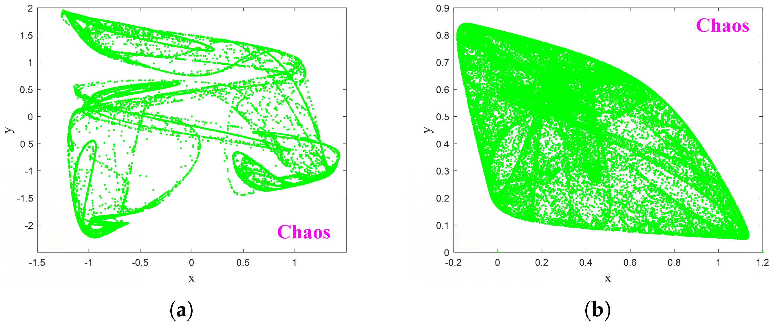
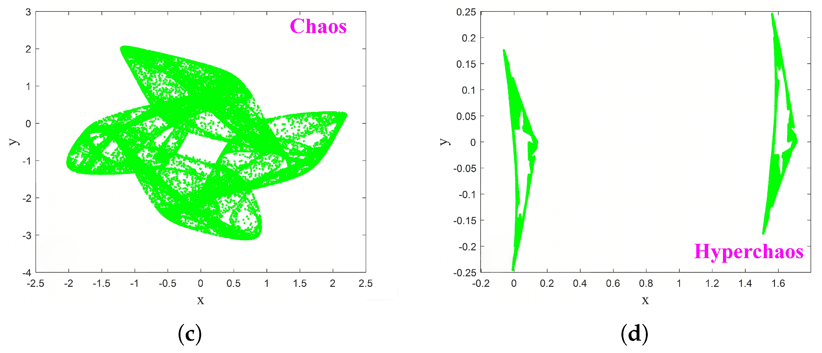
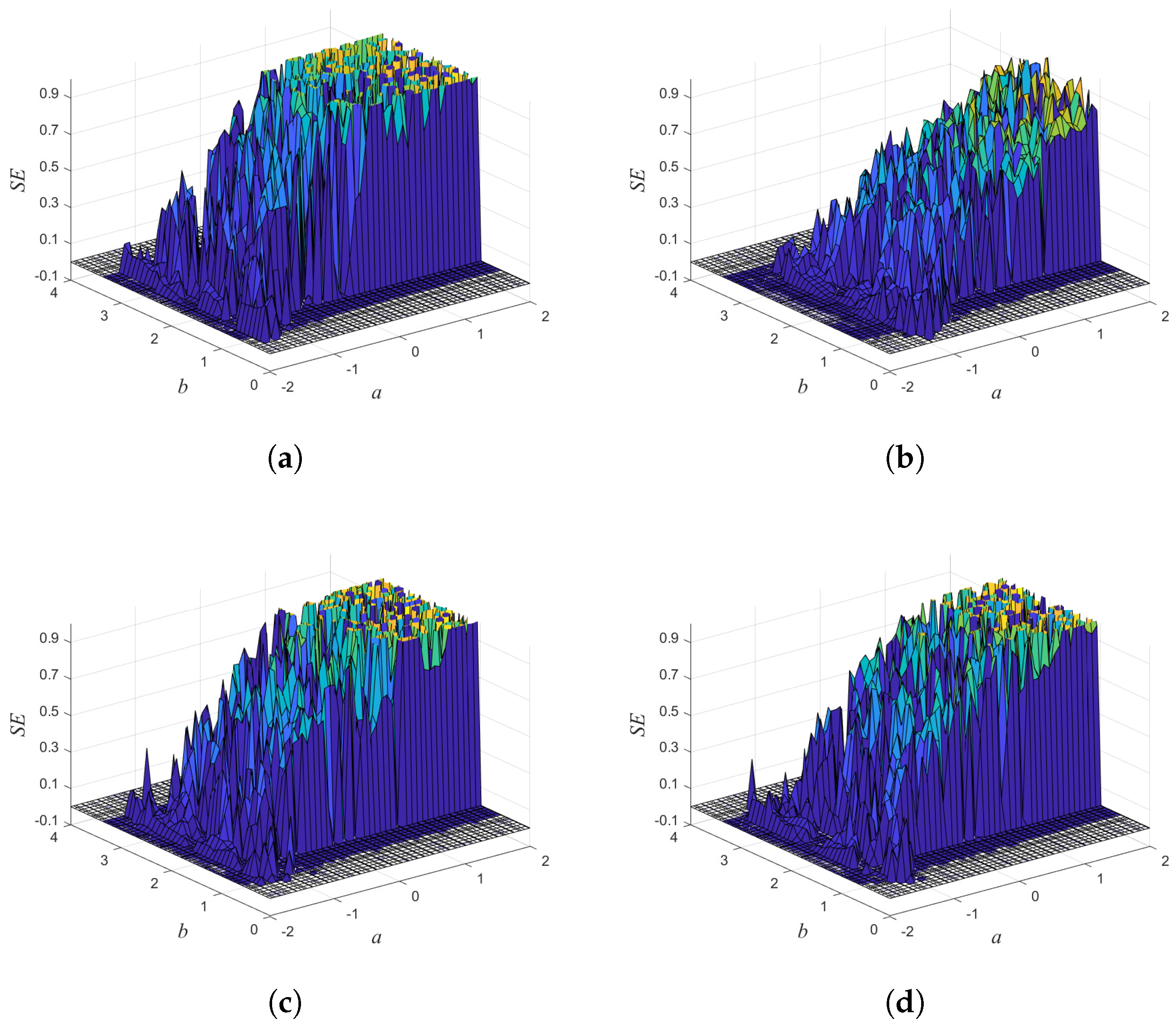
2.3. Bifurcation and LE Analysis

An essential tool for examining the features of a chaotic system is its bifurcation diagram. Under various control parameters, it may directly see the system’s chaotic state and period-doubling bifurcation. In phase space, the LE is a crucial metric for calculating the rate at which neighboring trajectories separate. In dynamical systems theory, the Lyapunov exponents (LEs) quantify the exponential divergence or convergence of neighboring trajectories, serving as a critical indicator of chaos. For a two-dimensional discrete dynamic system, the i-th Lyapunov exponent ${\lambda }_i$ (sorted by magnitude, $i=1,2$) is mathematically defined as

$${\lambda }_i=\underset{k\to \infty }{lim}{\displaystyle \frac{1}{k}}ln\left|{\mu }_i\left({\Phi }_k\right)\right|$$

(6)

where

${\mu }_i\left({\Phi }_k\right)$ denotes the i-th singular value of the cumulative Jacobian product matrix ${\Phi }_k$ (sorted in descending order); ${\Phi }_k$ is the state transition matrix over k iterations, constructed by multiplying the Jacobian matrices of the system at each discrete time step:

$${\Phi }_k=\prod _{l=0}^{k-1}J\left({\mathbf{x}}_l\right)$$

(7)

Here, $J\left({\mathbf{x}}_l\right)$ represents the Jacobian matrix of the system evaluated at the state ${\mathbf{x}}_l=(x\left(l\right),y\left(l\right))$ during the l-th iteration. The product ${\Phi }_k$ characterizes the linearized evolution of small perturbations around the trajectory $\{{\mathbf{x}}_0,{\mathbf{x}}_1,\dots ,{\mathbf{x}}_k\}$. We will talk about the system’s and the LEs’ bifurcation based on parameter values using the analysis from the previous section b. Assuming that $a=-1,c=0.65$, and $d=0.9$, we use $IC=(0,0)$ to examine how the system changes with parameter b and Figure 2 displays the associated LEs. The bifurcation diagram illustrates how the system’s trajectory progresses through periodic states, period-doubling bifurcations, and increasingly complex chaotic states as parameter b increases. This progression demonstrates how incremental parameter variation drives the system from ordered motion (negative LEs) through metastable bifurcations to fully developed chaos, where the exponential divergence of trajectories ensures sensitive dependence on initial conditions. Second, the associated LEs show that the system exhibits hyperchaotic behavior as well. The system’s trajectory in four distinct states is shown in Figure 3, which is in line with the analysis of the bifurcation diagram above.

2.4. Sample Entropy

The complexity of chaotic systems is quantified by the proximity of their sequences to random distributions, with sample entropy (SE) serving as a key metric for characterizing this property. A higher SE value indicates stronger stochastic irregularity in the time series, which directly correlates with the enhanced cryptographic security. For a given time series $\{l_1,l_2,\cdots ,l_n\}$, the SE is mathematically defined as

$$SE=-ln\left({\displaystyle \frac{A^m\left(r\right)}{B^m\left(r\right)}}\right)$$

(8)

where $A^m\left(r\right)$ denotes the average probability of m-dimensional vector pairs within a similarity threshold r; $B^m\left(r\right)$ denotes the average probability of $(m+1)$-dimensional vector pairs within the same threshold r; $d\left[X\right(i),X(j\left)\right]$ represents the Chebyshev distance between vectors $X\left(i\right)$ and $X\left(j\right)$, defined as $d[X\left(i\right),X\left(j\right)]={max}_{k=0}^{m-1}|x(i+k)-x(j+k)|$; $r=0.2\times \mathrm{std}$ (where std is the standard deviation of the time series) is the similarity threshold; $m=2$ is the conventional embedding dimension for phase-space reconstruction. Experimental results demonstrate that the proposed chaotic system achieves stable SE values asymptotically approaching 1 (Figure 4), exhibiting maximum entropy characteristics suitable for cryptographic applications. This verifies the system’s ideal unpredictability and security strength. The specific expressions for $A^m\left(r\right)$ and $B^m\left(r\right)$ are derived from the matching counts of phase-space vectors. For each i, the m-dimensional vector $A_i^m\left(r\right)$ is calculated as

$$A_i^m\left(r\right)={\displaystyle \frac{1}{N-m-1}}\sum _{\begin{array}{c}j=1j\ne i\end{array}}^{N-m}\Theta \left(r-d\left[X\right(i),X(j\left)\right]\right)$$

(9)

Similarly, the $(m+1)$-dimensional vector $B_i^m\left(r\right)$ is given by

$$B_i^m\left(r\right)={\displaystyle \frac{1}{N-m-1}}\sum _{\begin{array}{c}j=1j\ne i\end{array}}^{N-m}\Theta \left(r-d\left[X\right(i),X(j\left)\right]\right)$$

(10)

Here, $\Theta (·)$ is the Heaviside step function, where $\Theta \left(z\right)=1$ if $z\ge 0$ (indicating a match within threshold r) and $\Theta \left(z\right)=0$ otherwise; $X\left(i\right)=\left[x\right(i),x(i+1),\cdots ,x(i+m-1\left)\right]$ is the m-dimensional phase-space reconstruction vector (with $i=1,2,\cdots ,N-m+1$); the adaptive threshold $r=0.2\times \mathrm{std}$ ensures scale-invariant analysis across different dynamical systems [26].

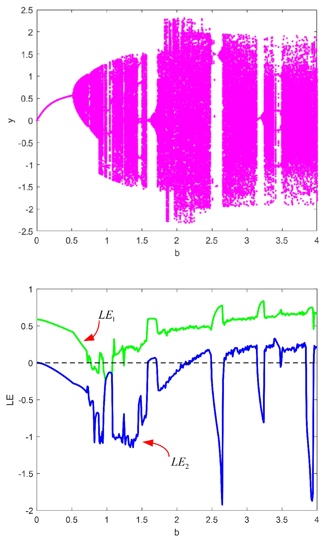
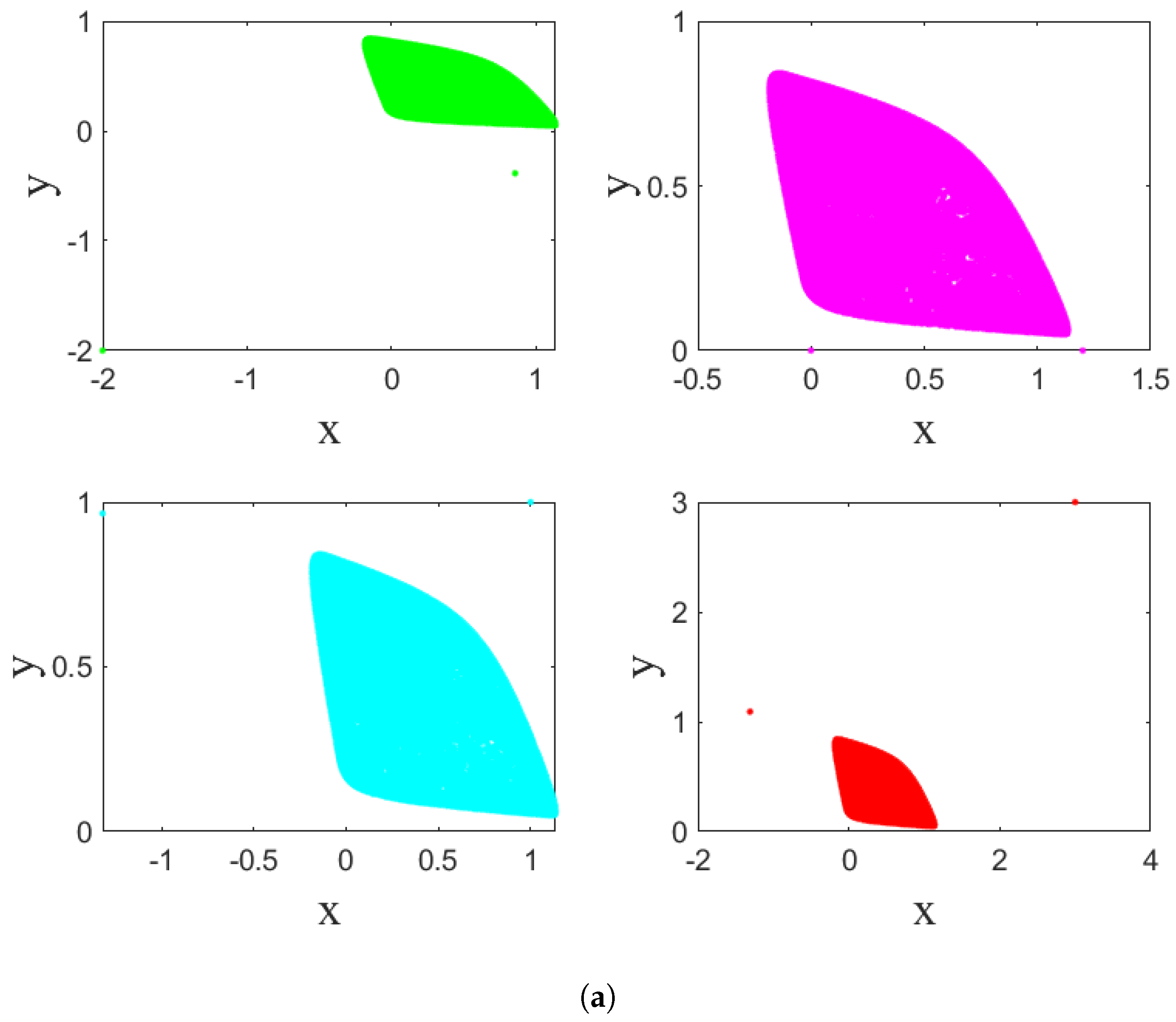
3. Homogeneous Multistability

The phenomenon known as homogeneous multistability characterizes chaotic systems that exhibit multiple stable attractors of identical geometric configuration, emerging from distinct initial conditions. The novel chaotic map embeds sinusoidal dynamics to leverage intrinsic periodicity, thereby enabling infinite attractor generation through phase space folding. Rigorous investigation under constant parameters reveals multistability, where distinct attractors and their phase orbits coexist across varied initialization domains.

The phase-space trajectories of the system under two distinct parameter configurations are analyzed: $a=-0.72$, $b=1$, $c=0.82$, $d=1.2$, with initial conditions $(x_0,y_0)=(0,0)$; $a=-1$, $b=1.7$, $c=0.65$, $d=0.9$, with initial conditions $(x_0,y_0)=(0.1,0.1)$. Figure 5 illustrates the corresponding attractors. Figure 5a is the first set of parameters given, and the initial values of the first row and column are $IC=(-2,-2)$; the initial values of the first row and second column are $IC=(0,0)$; the initial values of the second row and first column are $IC=(1,1)$; and the initial values of the second row and second column are $IC=(3,3)$. Figure 5b is the second set of parameters given, and the initial values of the first row and column are $IC=(-0.1,-0.1)$; the initial values of the first row and second column are $IC=(0,0)$; the initial values of the second row and first column are $IC=(0.1,0.1)$; and the initial values of the second row and second column are $IC=(0.2,0.2)$. This geometric consistency despite spatial relocation demonstrates the system’s ability to maintain deterministic chaos while exhibiting initial condition-dependent attractor positioning.

4. A Pseudorandom Number Generator Based on the Proposed Hyperchaotic System

Randomness constitutes a critical foundation for cryptographic systems and computational modeling, fundamentally categorized into two distinct generation paradigms: physical entropy sources (true randomness) and algorithmic simulations (pseudo-randomness). TRNGs rely on inherently stochastic physical phenomena—such as thermal fluctuations, quantum effects, or radioactive decay—to produce unpredictable sequences, ensuring entropy rooted in natural processes. This type of random number generation process is unpredictable, and the results are completely independent and cannot be copied, so they are widely used in such situations. In this paper, we use NIST SP 800-22 [37] standard test, which contains a variety of statistical tests, each of which focuses on the different characteristics of random sequences. Common test types include the following: Frequency test—checking whether the number of zeros and ones in the sequence is roughly equal. Block frequency test—checking whether the sub-blocks in the random sequence meet the expected frequency. Run-length test—analyzing the run-length distribution of consecutive identical numbers in a sequence. Poker test—check whether the combination of numbers in the sequence is random. Discrete Fourier transform (DFT) test—Detecting periodic patterns by analyzing the peaks in the frequency domain. Non-overlapping template matching test—15 common tests such as detecting whether the sequence matches a specific non-overlapping template to find the deviation [38]. Under a significance level of $\alpha =1\%$, sequences are deemed statistically random if their p-values satisfy $p\ge 0.01$ under NIST SP 800-22 criteria. Given the bounded output range $x\in (-5,5)$ of the proposed chaotic system, a pseudorandom number generator (PRNG) is constructed via the transformation:

$$\widehat{X}=\lfloor X·\mu \rfloor modN,$$

(11)

where $\lfloor ·\rfloor$ denotes the floor function, which extracts the greatest integer less than or equal to the operand. Scaling factor $\mu ={10}^4$ amplifies the system’s outputs to exploit full numerical precision. Modulus N controls the final digitization resolution. In this paper, we take the value of N as 256. Take X sequence, and its NIST test results are shown in

Table 1. The proposed system’s generated bitstream undergoes rigorous statistical validation through the test.

Order	Test Suites	p-Value	Result
1	Frequency	0.546821	Pass
2	Block frequency	0.765321	Pass
3	Cumulative sums (forward)	0.866744	Pass
4	Cumulative sums (backward)	0.123765	Pass
5	Runs	0.532570	Pass
6	Longest run	0.823465	Pass
7	Rank	0.972380	Pass
8	FFT	0.029687	Pass
9	Non-overlapping template	0.234758	Pass
10	Overlapping tempUniversal	0.166534	Pass
11	Universal	0.925643	Pass
12	Approximate entropy	0.614867	Pass
13	Random excursions	0.657103	Pass
14	Random excursions variant	0.587641	Pass
15	Serial (forward)	0.858761	Pass
16	Serial (backward)	0.762146	Pass
17	Linear complexity	0.714581	Pass

. As can be seen from Table 1, the sequence passed 15 pseudo-random tests. It further shows that the two-dimensional hyperchaotic system we constructed is random and can meet the requirements of cryptography for the randomness of keys.

5. A Color Image Encryption Scheme Based on 2D Hyperchaotic System and Its Corresponding Security Analysis

5.1. A Color Image Encryption Scheme Based on 2D Hyperchaotic System

The encryption scheme proposed in this section is based on “confusion” and “diffusion”. The confusion operation can shuffle the pixel position of the plaintext image, but it does not change the pixel value. The diffusion operation can change the value of pixels by invertible mapping. To achieve an optimal balance between security robustness and computational overhead, a dual-round permutation–diffusion cascade is strategically implemented. For color image processing, the encryption algorithm executes channel-wise transformations through the following protocol: The input image is decomposed into three distinct channels (R, G, B) through spectral separation. Each channel undergoes independent permutation and diffusion operations through the dual-round cascade. The processed channels are recombined through additive superposition to generate the final ciphertext image.

The decryption procedure constitutes an inverse transformation sequence, systematically reversing each cryptographic operation through inverse permutation matrices and complementary diffusion mappings. This bijective architecture ensures the perfect reconstruction of original image data when applying the correct decryption key.

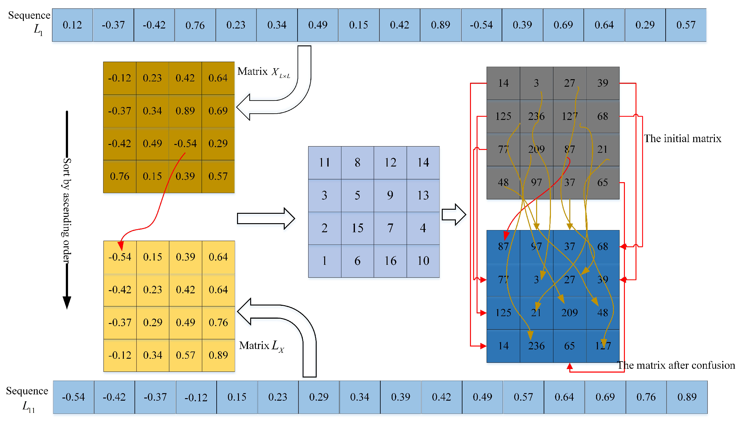
5.2. Confusion Operation

To enhance resistance against chosen plaintext attacks, the proposed scheme integrates a cryptographic hash function to dynamically bind the encryption process to the plaintext content. The security mechanism operates as follows:

$$\left\{\begin{array}{c}{x}_0^{\prime }=mod\left.(x_0+{\displaystyle \frac{h_0\oplus h_1\oplus h_2\oplus h_3}{32}},1\right)\hfill \\ y_0^{\prime }=mod\left.(y_0+{\displaystyle \frac{h_4\oplus h_5\oplus h_6\oplus h_7}{32}},1\right)\hfill \end{array}\right.$$

(12)

The cryptographic hash value $H=h_0\parallel h_1\parallel \cdots \parallel h_7$ (where $h_i\in {\{0,1\}}^{32}$) is generated from the plaintext image using SHA-256. Key specifications include the following: Each $h_i=b_0{b}_1\cdots b_{31}$ with $b_j\in \{0,1\}$ represents a 32-bit word. The $\parallel$ operator denotes bitwise concatenation. This configuration ensures the ΔP → ΔH avalanche effect exceeding 50% bit-flip probability per modified input bit. Because the chaotic sequence has the characteristics of non-repeatability, ergodicity, and randomness, if the generated chaotic sequence is sorted in ascending order, its index vector can be obtained. By recombining the obtained index vector into a matrix with the same size as the plaintext image by column, the pixels of the plaintext image can be scrambled according to the index matrix, and then the confusion operation can be realized. The specific confusion processing is shown in Algorithm 1. The confusion image can be generated by inputting a chaotic output sequence and plaintext image. To facilitate understanding, Figure 6 shows a concrete numerical example. The chaotic sequence is first truncated to a sequence L₁ of length 16, passing through an ascending sequence L₁₁, such as L₁₁(1) = −0.54, and L₁₁(1) = L₁(11) = −0.54. The sequences L₁ and L₁₁ are re-formed by columns into matrices $X_{L\times L}$ and $L_X$, then $L_X(1,1)=L_1\left(1\right)=-0.54=L_{11}\left(11\right), X_{L\times L}(3,3)=L_{11}\left(11\right)$. The first element of the index matrix’s intermediate matrix indicates that the element (value 87) from the original matrix’s (3, 3) position is mapped to the (1, 1) position of the new matrix. This mapping rule is uniformly applied to all elements. As shown in Figure 6, the permutation of all pixel positions in the matrix is evident. Usually, the matrix after rearrangement is called the matrix after confusion, that is, the effect of confusion is achieved.

Algorithm 1 Confusion during encryption

Input: the initial value {$x_0^{\prime }$, $y_0^{\prime }$}T of the chaotic system and the plaintext image P

Output: The image after confusion

1. According to the size of the plaintext image given, the intercepted chaotic sequence L1, L2 is arranged in ascending order, and the new sequence obtained is recorded as L11, L22

2. L11(i) = l1(index(i)). % index is the position element of sequence L11 in sequence L1

3. Reorganize L1, L2, L11, L22 into a square matrix by column, denoted as XL×L,YL×L, LX, LY, respectively.

4. For i from 1 to L do

5. For j from 1 to L do

6. $L_X(i,j)=L_{11}((j-1)L+i)$

7. $L_{11}((j-1)L+i)=L_1(index(j-1)L+i)$

8. $L_1(index(j-1)L+i)=X_{L\times L}(s,v)\%1\le s\le L,1\le vs.\le L$

9. $F_R(s,v)==P_R(i,j)\%$ Confused on color image R channel for operation

10. End for

11. End for

12. Similarly, $F_G(s,v)==P_G(i,j),F_B(s,v)==P_B(i,j)$

13. By recombining the three channels R, G and B, the image P after confusion can be obtained

5.3. Diffusion Operation

Diffusion operation involves changing the value of pixels through reversible mapping, which can achieve small differences in plaintext image pixels and make huge changes in ciphertext image. The pixel value of the spread image can be obtained using the previous pixel and the chaotic sequence to change the current pixel through a reversible map. The binary sequences X and Y can be converted to $\widehat{X}$ and $\widehat{Y}$, respectively. Furthermore, the confused image’s $R,G$, and B channel pixel locations are reshaped into column vectors one by one, represented as $R_{L\times L,1},G_{L\times L,1}$, $B_{L\times L,1}$, for example, ${\widehat{R}}_{L\times L,1},{\widehat{G}}_{L\times L,1}$, ${\widehat{B}}_{L\times L,1}$ represents the binary sequences created by converting the three sequences. The following diffusion equation can be used to encrypt the confused image.

$$\left\{\begin{array}{c}{C}_r\left(j\right)=\widehat{R}\left(j\right)\oplus \widehat{X}\left(j\right)\oplus \widehat{X}(j+1)j\in \{1,\cdots L^2-1\}\hfill \\ C_r\left(j\right)=\widehat{R}\left(j\right)\oplus \widehat{X}\left(j\right)\oplus \widehat{Y}\left(1\right)j=L^2\hfill \end{array}\right.$$

(13)

$$\left\{\begin{array}{c}{D}_r\left(j\right)=C_r\left(j\right)\oplus \widehat{X}\left(j\right)\oplus \widehat{Y}(j+1)\hfill \\ D_r\left(j\right)=C_r\left(j\right)\oplus \widehat{X}\left(j\right)\oplus \widehat{Y}\left(1\right)\hfill \end{array}\right.$$

(14)

Let $C_r\left(j\right)$ denote the pixel intensity at position j in the red (R) channel after forward diffusion processing, where nonlinear value propagation is achieved through chaotic mixing. Conversely, $D_r\left(j\right)$ corresponds to the reconstructed pixel value at position j following inverse diffusion operations, governed by $D_r\left(j\right)=F^{-1}\left(C_r\left(j\right)\right),j\in \{1,2,\cdots ,N\}$, where $F^{-1}$ represents the bijective inverse transformation that ensures perfect decryption fidelity when applied with correct cryptographic parameters. The two remaining channels of the color image can be obtained in the same way: for this purpose, the pixels of the three channels are integrated to obtain an encrypted image. The decryption procedure, which will not be explained here, is the opposite of the encryption process.

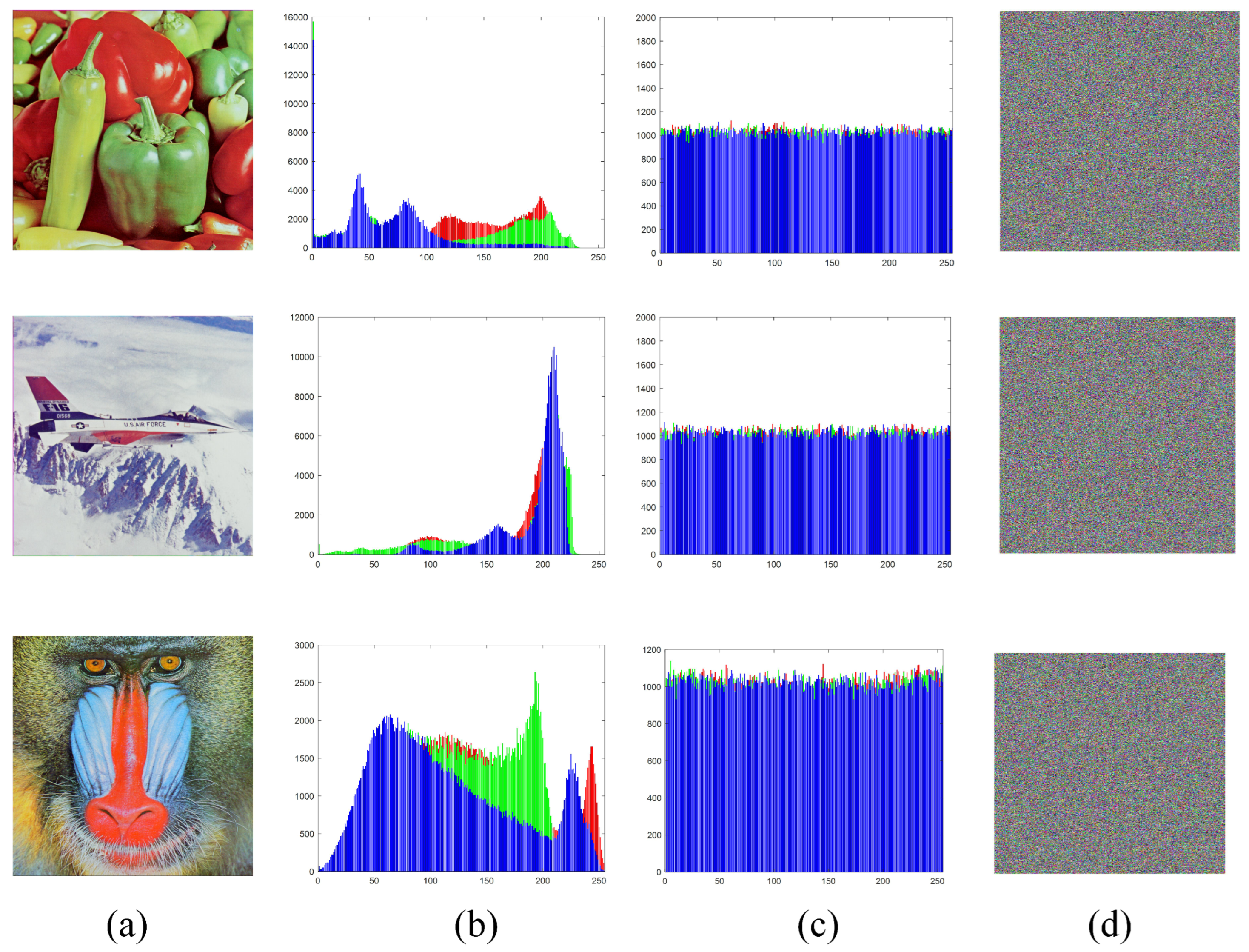
5.4. Simulation Results

To evaluate the proposed encryption scheme, three standard test images—Pepper, Airplane, and Monkey (RGB format, 512 × 512 pixels)—were selected as plaintext inputs. The algorithm was implemented in MATLAB R2018a on a Windows 10 platform equipped with an Intel^® Core™ i7-1180H processor (2.3 GHz) and 16 GB RAM. Figure 7 presents the encryption outcomes, demonstrating that the ciphertext images exhibit: histograms of the R, G, and B channels show statistically flat intensity distributions (Figure 7c), eliminating detectable patterns. No discernible traces of the plaintext content remain visible in the ciphertext domains (Figure 7d), confirming effective perceptual security. These results validate the scheme’s efficacy in ensuring both visual and statistical security through rigorous permutation–diffusion operations.

5.5. Security Analysis

5.5.1. Key Space Analysis

In order to meet the NIST SP 800-131A [39] requirement regarding resistance to brute-force attacks (where the key space must be greater than $2^{100}$), this encryption scheme utilizes a composite key structure. The security key is composed of core parameters $\{a,b,c,d\}\in \mathbb{R}$ and plaintext-dependent hash-bound components $\{x_0\oplus h,y_0\oplus h\}$, where $h=\mathrm{SHA}\text{-}256\left(P\right)$ represents the 256-bit hash value derived from the plaintext image P. Each key component is represented with 32-bit precision, yielding an effective key space of $2^{32\times 6}=2^{192}$. This surpasses the NIST minimum threshold of $2^{100}$ by a security margin of $2^{92}$ times. When validated against Kerckhoffs’ principle, the brute-force complexity remains $O\left(2^{192}\right)$ operations, even assuming full knowledge of the algorithm. This ensures resilience against all pre-quantum era exhaustive attacks.

5.5.2. Histogram Analysis and Information Entropy

As depicted in Figure 7, the pixels of the red (R), green (G), and blue (B) channels in the encrypted color image are relatively evenly distributed within the range of $[0,255]$. This implies that the probability of each pixel’s appearance is approximately equal. In contrast, the pixels of the original plaintext image are distributed in a regular pattern within the same range of $[0,255]$. Statistical analysis reveals a distinct divergence in pixel intensity distributions between the encrypted image and its original counterpart, with ciphertext histograms exhibiting uniform profiles devoid of discernible patterns characteristic of plaintext data. To further investigate the uniformity of the pixel distribution after encryption, this paper uses the chi-squared test for testing, whose expression is as follows:

$${\chi }^2=\sum _{i=0}^{255}{\displaystyle \frac{{(E_i-Z)}^2}{Z}}$$

(15)

where $E_i$ represents the frequency of the i-th pixel, and Z is the expected frequency of occurrence for each pixel. The expected frequency Z in statistics can be computed as

$$Z={\displaystyle \frac{M\times N}{256}}$$

(16)

with $M\times N$ being the image dimensions (number of pixels). The test results in

Table 2. The ${\chi }^2$-values of the encrypted color-images.

No.	Image	R	G	B	${\mathit{\chi }}_{255,0.05}^2=310.457$	${\mathit{\chi }}_{255,0.01}^2=293.2478$
1	Pepper	274.67	252.17	246.98	pass	pass
2	Airplane	261.23	249.09	258.92	pass	pass
3	Monkey	253.18	250.01	257.98	pass	pass

demonstrate that the proposed encryption scheme satisfies the null hypothesis at both 5% and 1% significance levels ($\alpha =0.05$ and $\alpha =0.01$), confirming a statistically uniform gray-level distribution in ciphertext histograms. The ${\chi }^2$ statistics for all three channels (R, G, B) are below the critical value at $\alpha =0.01$, indicating no significant deviation from uniformity.

The Shannon entropy is employed to assess whether an encrypted image exhibits random-like characteristics, serving as a means to quantify the information content within the images. It is defined as follows:

$$H\left(S\right)=-\sum _{i=0}^{2^n-1}P\left(S_i\right){log}_2\left|P\left(S_i\right)\right|,$$

(17)

where n represents the bit depth of the image, and $P\left(S_i\right)$ denotes the discrete probability density function of the pixel value $s_i$. When the bit depth $n=8$, the optimal information entropy value is $H\left(s\right)=8$.

Table 3. The information entropy of the encrypted images.

Encrypted Images	Pepper	Airplane	Monkey
Ref. [38]	7.99950	7.99950	7.99940
Ref. [40]	7.99934	7.99932	7.99933
Ref. [41]	7.99940	7.99930	7.99940
Ref. [42]	7.99920	7.99900	7.99940
Our scheme	7.99923	7.99910	7.99940

provides a comparative analysis of the information entropy values across various encryption techniques. The proposed encryption algorithm attains an average Shannon entropy of $7.9992\pm 0.0003$ for the ciphertext images. This value closely approaches the theoretical maximum of $8.0$ for 8-bit systems, highlighting its superior ability to maximize entropy in comparison to existing encryption schemes. Furthermore, the convergence to ideal entropy values, coupled with histogram uniformity metrics (Section 5.2), confirms the algorithm’s efficacy in achieving cryptographic-grade diffusion through nonlinear transformations.

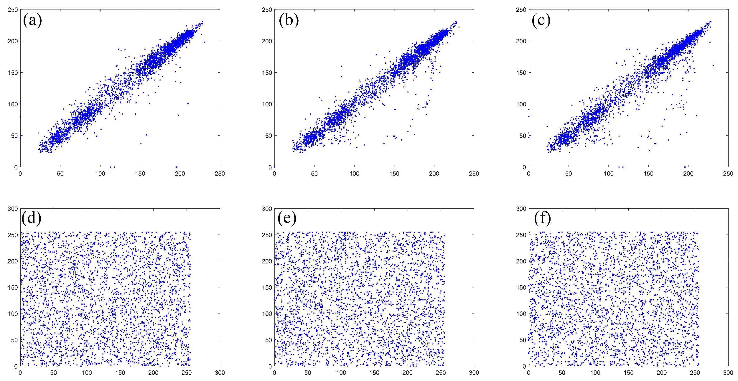
5.5.3. Correlation Analysis

Natural color imagery inherently maintains strong chromatic coherence across RGB spectral channels, manifested through pronounced intensity congruence among spatially adjacent pixels. This structural redundancy necessitates cryptographic systems to implement decorrelative transformations that attenuate plaintext pixel dependencies while establishing stochastic decorrelation in ciphertexts. The security objective requires reducing inter-pixel Pearson correlation coefficients from initial values ${\rho }_{\mathrm{plain}}\approx 0.9$ to cryptographically secure levels ${\rho }_{\mathrm{cipher}}<0.01$ through nonlinear diffusion mechanisms. The Pearson correlation coefficient ${\rho }_{xy}$ quantifies linear dependencies between adjacent pixel pairs $(x,y)$, computed through the following statistical measures:

$$\left\{\begin{array}{c}E\left(x\right)={\displaystyle \frac{1}{N}}{\displaystyle \sum _{i=1}^N}{x}_i\hfill \\ D\left(x\right)={\displaystyle \frac{1}{N}}{\displaystyle \sum _{i=1}^N}{\left[x_i-E\left(x\right)\right]}^2\hfill \\ cov(x,y)={\displaystyle \frac{1}{N}}{\displaystyle \sum _{i=1}^N}\left[x_i-E\left(x\right)\right]\left[y_i-E\left(y\right)\right]\hfill \\ {\rho }_{xy}={\displaystyle \frac{cov(x,y)}{\sqrt{D\left(x\right)}\sqrt{D\left(y\right)}}}\hfill \end{array}\right.$$

(18)

where N denotes the number of adjacent pixel pairs analyzed, $E(·)$ and $D(·)$ represent the expectation and variance operators, respectively, and $x,y$ correspond to neighboring pixel intensity values. Generally, the lower the correlation between adjacent pixels, the more effective the encryption. Taking the red channel of a color image as an example, Figure 8 illustrates the distribution of adjacent pixel pairs of both the original image and the encrypted image in three directions: horizontal, vertical, and diagonal. As depicted in Figure 8, 3000 pairs of adjacent pixels in the original image display a concentrated distribution along a single line in all three directions. In stark contrast, the 3000 pairs of adjacent pixels in the encrypted image are evenly distributed within the value range across these directions, without any signs of clustering or dispersion. This observation strongly suggests that the proposed encryption scheme can effectively achieve excellent diffusion characteristics.

Table 4. The comparison of the results of the correlation analysis of the encryption schemes.

Pepper	Original Image			Encrypted Image
	Horizontal	Vertical	Diagonal	Horizontal	Vertical	Diagonal
Ref. [43]	0.9783	0.9789	0.9661	0.0031	0.0014	0.0006
Ref. [44]	0.9783	0.9789	0.9661	−0.0041	−0.0024	0.0007
Ref. [45]	0.9783	0.9789	0.9661	−0.0023	−0.0036	0.0021
Ref. [46]	0.9783	0.9789	0.9661	0.0019	0.0036	0.0017
Our scheme	0.9783	0.9789	0.9661	−0.0005	0.0009	0.0010

presents the correlation coefficients between the images encrypted by different encryption schemes and the original plaintext images. It is clearly observable that the correlation coefficients of the original image are close to 1 in all three directions (horizontal, vertical, and diagonal), while those of the encrypted images approach 0 asymptotically. This indicates that the encrypted image has a negligible inter-pixel correlation in the horizontal, vertical, and diagonal orientations. A comparative analysis with existing encryption schemes reveals that the correlation values of images encrypted using the proposed method are consistently lower across all directions. These results strongly imply that the proposed encryption scheme provides enhanced resistance against correlation-based attacks.

5.5.4. Differential Attack

The diffusion operation employs bijective transformations to induce stochastic pixel value perturbations through nonlinear coupling between chaotic sequences and preceding pixel values. This triggers an avalanche effect where minimal plaintext variations ($\Delta P\ge 1$ bit) propagate into global ciphertext alterations ($\Delta C\propto N_{\mathrm{pixels}}$). The diffusion efficiency is quantified via NPCR (number of pixels change rate) and UACI (unified average changing intensity) [32]:

$$\left\{\begin{array}{c}NPCR={\displaystyle \frac{{\displaystyle \sum _{m=1}^M}{\displaystyle \sum _{n=1}^N}D(m,n)}{MN}}\times 100\%\hfill \\ UACI={\displaystyle \sum _{m=1}^M}{\displaystyle \sum _{n=1}^N}{\displaystyle \frac{\left|c_1(m,n)-c_2(m,n)\right|}{255\times MN}}\times 100\%\hfill \end{array}\right.$$

(19)

The differential metrics are computed as

$$\left\{\begin{array}{c}D(m,n)=\left\{\begin{array}{cc}1\hfill & C_1(m,n)\ne C_2(m,n)\hfill \\ 0\hfill & \mathrm{otherwise}\hfill \end{array}\right.\hfill \\ c_k(m,n)\in {\mathbb{Z}}_{256}\forall (m,n)\in [1,M]\times [1,N]\hfill \end{array}\right.$$

where $C_k$ denotes the ciphertext images generated from single-bit-differing plaintexts, with $M\times N$ representing spatial resolution. The average values of both the number of pixels change rate ($\mathrm{NPCR}\approx 99.6094$) and the unified average changing intensity ($\mathrm{UACI}\approx 33.463507$) are approaching the ideal expected values [47]. This suggests that the algorithm possesses strong resilience against differential attacks.

Table 5. The values of NPCR and UACI of the encrypted images.

Images	NPCR(%)			UACI(%)
	R	G	B	R	G	B
Pepper	99.63	99.63	99.60	33.42	33.46	33.50
Airplane	99.65	99.59	99.63	33.40	33.28	33.28
Monkey	99.59	99.58	99.62	33.37	33.32	33.30

presents the comparison results between this algorithm and other encryption schemes. It is evident from the results that the algorithm proposed in this research surpasses the existing methods. Specifically, it shows a more significant closeness to the ideal expected values for both the NPCR and UACI metrics, which serves as solid evidence of its superiority. These findings provide additional confirmation of the algorithm’s exceptional ability to resist differential attacks, highlighting its enhanced performance in comparison to other approaches.

5.5.5. Time Analysis

Because the system is a discrete-time model, that is, a difference equation. So, the time complexity of this part is $O\left(n\right)$, where $n=L^2$. The confusing part is the indexed sequential lookup problem, which has a complexity of $O(nlogn)$. The diffusion part is a cycle of n degrees, and the complexity of this part is also $O\left(n\right)$. In addition, the complexity of the hash function is $O\left(1\right)$. Then, the time complexity of the scheme is $O(nlogn)$. The effectiveness of the encryption technique is also significantly measured by the time complexity, based on the AMD Ryzen 7 5800H 3.20 GHz CPU model and the modeling environment is Matlab 2021a. Besides security analysis, the time efficiency of the encryption algorithm serves as a crucial performance metric.

Table 6. Running time of different images.

Image	Size	Encryption Time (s)	Decryption Time (s)
Peppers	$128\times 128$	0.202145	0.284039
	$256\times 256$	0.324531	0.385432
	$512\times 512$	0.426432	0.503421
	$1440\times 900$	0.893421	0.983241

displays the time required for the encryption and decryption of color images of varying sizes using the proposed encryption algorithm. Table 6 provides a comparative analysis of the time efficiency between the proposed algorithm and similar algorithms when encrypting the Peppers ($128\times 128$, $256\times 256$, $512\times 512$ and $1440\times 900$) images.

6. Conclusions

This work suggests a 2D hyperchaotic system with a hyperchaotic map that has configurable coexisting attractors, aiming to better adapt the chaotic system to engineering applications. Specifically, by adding orthorhombic feedback, the dynamic features demonstrate the system’s rich dynamic nature. Furthermore, the suggested hyperchaotic maps with orthorhombic feedback exhibit homogeneous multistability, or an infinite number of coexisting attractors. Based on extensive numerical simulations that demonstrate the system’s complex nonlinear dynamics and cryptographic grade stochasticity, we develop a color image encryption scheme employing a three-phase permutation–diffusion architecture. Security analysis indicates that the proposed map performs effectively in the realm of image encryption.

References

1. Rakkiyappan, R.; Chandrasekar, A.; Lakshmanan, S. Effects of leakage time-varying delays in Markovian jump neural networks with impulse control. Neurocomputing 2013, 121, 365–378. [Google Scholar] [CrossRef]
2. Rakkiyappan, R.; Chandrasekar, A.; Lakshmanan, S. Exponential stability of Markovian jumping stochastic Cohen-Grossberg neural networks with mode-dependent probabilistic time-varying delays and impulses. Neurocomputing 2014, 131, 265–277. [Google Scholar] [CrossRef]
3. Yan, W.; Jiang, Z.; Huang, X.; Ding, Q. Adaptive Neural Network Synchronization Control for Uncertain Fractional-Order Time-Delay Chaotic Systems. Fractal Fract. 2023, 7, 288. [Google Scholar] [CrossRef]
4. Deng, Y.M.; Fan, H.F.; Wu, S.M. A hybrid ARIMA-LSTM model optimized by BP in the forecast of outpatient visits. J. Ambient Intell. Humaniz. Comput. 2020, 14, 5517–5527. [Google Scholar] [CrossRef]
5. Xu, G.; Xu, J.; Xiu, C.; Liu, F.; Zang, Y. Secure communication based on the synchronous control of hysteretic chaotic neuron. Neurocomputing 2017, 227, 108–112. [Google Scholar] [CrossRef]
6. Wu, A.; Zeng, Z. Dynamic behaviors of memristor-based recurrent neural networks with time-varying delays. Neural Netw. 2012, 36, 1–10. [Google Scholar] [CrossRef] [PubMed]
7. Devaney, R.L. An Introduction to Chaos Dynamical Systems; Addison Wesley Publishing Company: New York, NY, USA, 1989. [Google Scholar]
8. Elwakil, A.S.; Kennedy, M.P. Chua’s circuit decomposition: A systematic design approach for chaotic oscillators. J. Frankl. Inst. 2000, 337, 251–265. [Google Scholar] [CrossRef]
9. Salamon, M. Chaotic electronic circuits in cryptography. In Applied Cryptography and Network Security; IntechOpen: London, UK, 2012. [Google Scholar] [CrossRef]
10. Bao, B.; Hu, J.; Cai, J.; Zhang, X.; Bao, H. Memristor-induced mode transitions and extreme multistability in a map-based neuron model. Nonlinear Dyn. 2023, 111, 3765–3779. [Google Scholar] [CrossRef]
11. Bao, H.; Hua, M.; Ma, J.; Chen, M.; Bao, B. Offset-control plane coexisting behaviors in two-memristor-based Hopfield neural network. IEEE Trans. Ind. Electron. 2023, 70, 10526–10535. [Google Scholar] [CrossRef]
12. Li, C.; Lei, T.; Liu, Z. Offset parameter cancellation produces countless coexisting attractors. Chaos Interdiscipl. J. Nonlinear Sci. 2022, 32, 121104. [Google Scholar] [CrossRef]
13. Csaba, G.; Porod, W. Coupled oscillators for computing: A review and perspective. Appl. Phys. Rev. 2020, 7, 011302. [Google Scholar] [CrossRef]
14. Li, C.; Sprott, J. Amplitude control approach for chaotic signals. Nonlinear Dyn. 2013, 73, 1335–1341. [Google Scholar] [CrossRef]
15. Li, C.; Sprott, J. Variable-boostable chaotic flows. Optik 2016, 127, 10389–10398. [Google Scholar] [CrossRef]
16. Lin, H.; Wang, C. Influences of electromagnetic radiation distribution on chaotic dynamics of a neural network. Appl. Math. Comput. 2020, 369, 124840. [Google Scholar] [CrossRef]
17. Sambas, A.; Vaidyanathan, S.; Zhang, X.; Koyuncu, I.; Bonny, T.; Tuna, M.; Alçin, M.; Zhang, S.; Sulaiman, I.M.; Awwal, A.M.; et al. A novel 3D chaotic system with line equilibrium: Multistability, integral sliding mode control, electronic circuit, FPGA implementation and its image encryption. IEEE Access 2022, 10, 68057–68074. [Google Scholar] [CrossRef]
18. Fan, C.; Ding, Q.; Tse, C.K. Designing n-D non-degenerate hyperchaotic systems via a simple circulant matrix. IEEE Trans. Circuits Syst. II Exp. Briefs 2024, 71, 460–464. [Google Scholar] [CrossRef]
19. Wang, M.; Gu, L. Multiple mixed state variable incremental integration for reconstructing extreme multistability in a novel memristive hyperchaotic jerk system with multiple cubic nonlinearity. Chin. Phys. B 2024, 33, 020504. [Google Scholar] [CrossRef]
20. Lai, Q.; Yang, L.; Liu, Y. Design and realization of discrete memristive hyperchaotic map with application in image encryption. Chaos Solitons Fractals 2022, 165, 112781. [Google Scholar] [CrossRef]
21. Wei, Z.; Zhang, W. Hidden hyperchaotic attractors in a modiffed Lorenz–Stenffo system with only one stable equilibrium. Int. J. Bifurc. Chaos 2014, 24, 1450127. [Google Scholar] [CrossRef]
22. Minati, L. Simulation versus experiment in non-linear dynamical systems. Chaos Solitons Fractals 2021, 144, 110656. [Google Scholar] [CrossRef]
23. Cao, W.; Cai, H.; Hua, Z. n-dimensional chaotic map with application in secure communication. Chaos Solitons Fractals 2022, 163, 112519. [Google Scholar] [CrossRef]
24. Zhao, Y.; Ding, J.; He, S.; Wang, H.; Sun, K. Fully fixedpoint integrated digital circuit design of discrete memristive systems. AEU-Int. J. Electron. Commun. 2023, 161, 154522. [Google Scholar] [CrossRef]
25. He, S.; Fu, L.; Yao, L.; Wu, X.; Wang, H.; Sun, K. Analog circuit of a simplified tent map and its application in sensor position optimization. IEEE Trans. Circuits Syst. II Express Briefs 2022, 70, 885–888. [Google Scholar] [CrossRef]
26. Yan, W.; Ding, Q. n-dimensional polynomial hyperchaotic systems with synchronization application. Eur. Phys. J. Plus 2023, 138, 915. [Google Scholar] [CrossRef]
27. Cai, Z.; Sun, J. Convergence of C0 complexity. Int. J. Bifurc. Chaos 2009, 19, 977–992. [Google Scholar] [CrossRef]
28. Tomcala, J. New fast ApEn and SampEn entropy algorithms implementation and their application to supercomputer power consumption. Entropy 2020, 22, 863. [Google Scholar] [CrossRef]
29. Li, C.B.; Sprott, J.C.; Xing, H. Constructing chaotic systems with conditional symmetry. Nonlinear Dyn. 2016, 87, 1351–1358. [Google Scholar] [CrossRef]
30. Fan, C.L.; Ding, Q. A universal method for constructing non-degenerate hyperchaotic systems with any desired number of positive Lyapunov exponents. Chaos Solit. Fractals 2022, 161, 112323. [Google Scholar] [CrossRef]
31. Belazi, A.; Khan, M.; El-Latif, A.A.A.; Belghith, S. Efficient cryptosystem approaches: S-boxes and permutation-substitution-based encryption. Nonlinear Dyn. 2017, 87, 337–361. [Google Scholar] [CrossRef]
32. Hua, Z.Y.; Zhou, Y.C. Design of image cipher using block-based scrambling and image filtering. Inf. Sci. 2017, 396, 97–113. [Google Scholar] [CrossRef]
33. Cao, C.; Sun, K.; Liu, W. A novel bit-level image encryption algorithm based on 2D-LICM hyperchaotic map. Signal Process 2018, 143, 122–133. [Google Scholar] [CrossRef]
34. Lu, L.; Li, Y.; Sun, A. Parameter identification and chaos synchronization for uncertain coupled map lattices. Nonlinear Dyn. 2013, 73, 2111–2117. [Google Scholar] [CrossRef]
35. Ronneberger, O.; Fischer, P.; Brox, T. U-Net: Convolutional Networks for Biomedical Image Segmentation. In Medical Image Computing and Computer-Assisted Intervention–MICCAI 2015: 18th International Conference, Munich, Germany, 5–9 October 2015, Proceedings, Part III 18; Springer: Cham, Switzerland, 2015. [Google Scholar]
36. Wu, S.; Zhong, S.; Liu, Y. Deep residual learning for image steganalysis. Multimed. Tools Appl. 2017, 77, 10437–10453. [Google Scholar] [CrossRef]
37. NIST SP 800-22 Rev. 1a; A Statistical Test Suite for Random and Pseudorandom Number Generators for Cryptographic Applications. NIST: Gaithersburg, MD, USA, 2010.
38. Raghuvanshi, A.; Budhia, M.; Patro, K.A.K.; Acharya, B. FSR-SPD: An efficient chaotic multi-image encryption system based on flip-shift-rotate synchronous-permutation-diffusion operation. Multimed. Tools Appl. 2024, 83, 57011–57057. [Google Scholar] [CrossRef]
39. NIST SP 800-131A Rev. 2; Offset Parameter Cancellation and Cryptographic Algorithm Transition Guidance. NIST: Gaithersburg, MD, USA, 2019. [CrossRef]
40. Yan, X.; Hu, Q.; Teng, L. A novel color image encryption method based on new three-dimensional chaotic mapping and DNA coding. Nonlinear Dyn. 2025, 113, 1799–1826. [Google Scholar] [CrossRef]
41. Acharya, B.; Sravan, J.V.; Potnuru, D.J.R.; Patro, K.A.K. MIE-SPD: A New and Highly Efficient Chaos-Based Multiple Image Encryption Technique With Synchronous Permutation Diffusion. IEEE Access 2025, 13, 3558943. [Google Scholar] [CrossRef]
42. Yan, W.; Ding, Q. A controllable 3D hyperchaotic map with infinite coexisting attractors and its application to image encryption. Nonlinear Dyn. 2024, 113, 9045–9059. [Google Scholar] [CrossRef]
43. Liu, C.Y.; Ding, Q. A color image encryption scheme based on a novel 3d chaotic mapping. Complexity 2020, 202, 3837209. [Google Scholar] [CrossRef]
44. Hua, Z.Y.; Cheng, Y.Y.; Bao, H.; Zhou, Y.C. Two-dimensional parametric polynomial chaotic system. IEEE Trans. Cybern. 2022, 52, 4402–4414. [Google Scholar] [CrossRef]
45. Xin, Y.; Wang, X. Fractal sorting matrix and its application on chaotic image encryption. Inf. Sci. 2021, 547, 1154–1169. [Google Scholar] [CrossRef]
46. Xu, Q.; Sun, K.; Zhu, C. A visually secure asymmetric image encryption scheme based on RSA algorithm and hyperchaotic map. Phys. Scrpta 2020, 95, 035223. [Google Scholar] [CrossRef]
47. Zhou, Y.C.; Bao, L.; Chen, C.L.P. A new 1D chaotic map for image encryption. Signal Process 2014, 97, 3039–3052. [Google Scholar] [CrossRef]
Figure 1. The outputs the motion trajectory of the system (1) with different control parameters and I C = ( 0 , 0 ) : (a) a = 0.72 , b = 1 , c = 0.82 and d = 1.2 ; (b) a = 0.82 , b = 1.2 , c = 0.42 and d = 0.6 ; (c) a = 0.2 , b = 1.2 , c = 0.7 and d = 1 ; and (d) a = 1 , b = 1.7 , c = 0.65 , d = 0.9 .
Symmetry 17 00801 g001aSymmetry 17 00801 g001b
Figure 2. Under the initial condition I C = ( 0 , 0 ) and fixed system parameters, the bifurcation analysis and Lyapunov exponent (LE) spectrum of System ( 1 ) are investigated as parameter b varies.
Symmetry 17 00801 g002
Figure 3. The motion trajectories of System ( 1 ) and their corresponding outputs, with the parameter b changing, are shown below under the initial condition I C = ( 0 , 0 ) and the fixed parameters a = 1 , c = 0.65 , and d = 0.9 (a) b = 0.7 , (b) b = 1.1 , (c) b = 1.65 , (d) b = 1.72 .
Symmetry 17 00801 g003
Figure 4. The sample entropy of the system (1) with a , b changes under I C = 0 , 0 : (a) c = 0.82 and d = 1.2 , (b) c = 0.42 and d = 0.6 , (c) c = 0.7 , and d = 1 , (d) c = 0.65 , d = 0.9 .
Symmetry 17 00801 g004
Figure 5. The coexistence of multiple attractors of system (1) with I C changes: (a) system (1) with a = 0.72 , b = 1 , c = 0.82 , d = 1.2 ; and (b) system (1) with a = 1 , b = 1.7 , c = 0.65 , d = 0.9 .
Symmetry 17 00801 g005aSymmetry 17 00801 g005b
Figure 6. A numerical example of confusion part.
Symmetry 17 00801 g006
Figure 7. The simulation results: (a) the plaintext images; (b) the histograms of plaintext images; (c) the histograms of the images after encryption; and (d) the encrypted images after encryption.
Symmetry 17 00801 g007
Figure 8. The arrangement of neighboring pixels: (a) The horizontal direction of original image; (b) The vertical direction of original image; (c) The diagonal direction of original image; (d) The horizontal direction of the encrypted image; (e) The vertical direction of the encrypted image; and (f) The diagonal direction of encrypted image.
Symmetry 17 00801 g008