Closed Forms and Structural Properties of Lucas Matrices Derived from Tridiagonal Toeplitz Matrices

Abstract

This study investigates the closed forms of Lucas matrices, with a particular emphasis on the $n^{th}$ powers of the tridiagonal symmetric Toeplitz matrix $S_4(x,y)$, whose entries are associated with Lucas numbers $L_n$. The analysis extends Filipponi’s foundational work by examining distinct cases of ordered pairs $(x,y)$, thereby determining the precise conditions under which $S_4(x,y)$ qualifies as a Fibonacci–Lucas matrix. Furthermore, it identifies specific conditions under which $S_4(x,y)$ can be classified as any Fibonacci–Lucas matrix. These findings contribute to the theoretical framework of Fibonacci–Lucas matrices and provide novel insights into their structural properties.

1. Introduction

The Lucas number $L_n$ is defined with the recurrence relation $L_n=L_{n-1}+L_{n-2}$, $n\ge 2$ for the initial values $L_0=2$, $L_1=1$. Similarly, the Fibonacci numbers are defined by the same recurrence relation for initial values $F_0=0$, $F_1=1$. In addition, both sequences are given by the Binet formulas,

$$L_n={\alpha }^n+{\beta }^n,F_n={\displaystyle \frac{{\alpha }^n-{\beta }^n}{\alpha -\beta }},$$

(1)

where $\alpha =\left(1+\sqrt{5}\right)/2$ known as the golden ratio and $\beta =\left(1-\sqrt{5}\right)/2$, $\beta =-{\alpha }^{-1}$. In the literature, a number of authors have provided alternative proofs for fundamental identities involving Lucas and Fibonacci numbers by employing methods from number theory, geometry, matrix theory, and related fields. Among these methods, the Binet formulas are frequently employed in the proofs of various interesting properties presented below, such as the following:

$$\begin{array}{ccc}\hfill L_{-n}& =& {\left(-1\right)}^n{L}_n,F_{-n}={\left(-1\right)}^{n+1}{F}_n\hfill \end{array}$$

(2)

$$\begin{array}{ccc}\hfill L_n& =& F_{n-1}+F_{n+1},5F_n=L_{n-1}+L_{n+1}.\hfill \end{array}$$

(3)

Furthermore, the powers of $\alpha$ and $\beta$ also satisfy similar recurrence relations and are closely related to the Lucas numbers as follows:

$$\begin{array}{ccc}& & \begin{array}{cc}{\alpha }^n={\alpha }^{n-1}+{\alpha }^{n-2},& {\beta }^n={\beta }^{n-1}+{\beta }^{n-2},\end{array}\hfill \end{array}$$

(4)

$$\begin{array}{ccc}& & \begin{array}{cc}\sqrt{5}{\alpha }^n=\alpha L_n+L_{n-1},& -\sqrt{5}{\beta }^n=\beta L_n+L_{n-1},\end{array}\hfill \end{array}$$

(5)

$$\begin{array}{ccc}& & \begin{array}{cc}\sqrt{5}{\beta }^n=\alpha L_n-L_{n+1},& \sqrt{5}{\alpha }^n=L_{n+1}-\beta L_n.\end{array}\hfill \end{array}$$

(6)

The golden ratio, along with the Fibonacci and Lucas numbers, has been studied extensively in a wide range of mathematical and geometric contexts. Key areas of research include the fundamental properties of the golden ratio, its applications to geometric problems in both two- and three-dimensional spaces, and its connections to the Fibonacci $F_n$ and Lucas $L_n$ numbers, along with their generalizations. The studies highlight numerous applications of these numbers in various fields such as mathematics, physics, biology, and engineering, demonstrating their interdisciplinary significance [1,2], for example, the regular pentagon and the fifth roots of unity reveal geometric relationships with the golden ratio, as illustrated in Table 1.

Table 1. The golden ratio with the fifth roots of unity.

j	1	2	3	4
$2cos\left(\frac{j\pi }{5}\right)$	$\alpha$	$-\beta$	$\beta$	$-\alpha$

Where symbol $\alpha =\left(1+\sqrt{5}\right)/2$ denotes the golden ratio and $1-\alpha =\beta$. For more detailed information, see [1,2,3].

Some matrices whose exponent entries are related to Fibonacci $F_n$ and/or Lucas $L_n$ numbers are called Fibonacci or Lucas matrices. The Fibonacci matrix Q was first introduced by King in his master’s thesis, and its generalizations have been extensively studied in subsequent research in [2,4]. Later, an application of the Lucas $Q_L$ matrix to Lucas numbers was presented in [5]. This approach led to the investigation of several properties, which can be expressed through the following matrix powers:

$$Q_L=\left(\begin{array}{cc}{L}_2& L_1\\ L_1& L_0\end{array}\right),Q_L^{2n}=5^n\left(\begin{array}{cc}{F}_{2n+1}& F_{2n}\\ F_{2n}& F_{2n-1}\end{array}\right),Q_L^{2n+1}=5^n\left(\begin{array}{cc}{L}_{2n+2}& L_{2n+1}\\ L_{2n+1}& L_{2n}\end{array}\right).$$

For example, Cassini’s formulas are derived through the determinant $det\left(Q_L^n\right)$. Moreover, the derivation of numerous Fibonacci and Lucas identities is based on matrix equations such as $Q_L^m{Q}_L^n=Q_L^{m+n}$ and $Q_L^m{Q}_L^{-n}=Q_L^{m-n}$, which provide a foundational framework for these studies.

Matrix methods have been widely used to derive new identities that involve the Fibonacci and Lucas numbers in [4,5,6,7,8,9,10,11,12,13,14,15,16]. For example, the Pascal matrix R was used to establish identities connecting these numbers in [6]. The relationships between Fibonacci or Lucas numbers and the Pascal matrix were explored, yielding closed-form expressions for $R_L^n$ and ${(R_L-5I)}^n$ in [7].

In [17], the author demonstrated the versatility of matrix analogues of the binomial and Waring formulas using generalized Fibonacci matrices. Washington [18] investigated $4\times 4$ Fibonacci matrices, highlighting their connections to the fifth roots of unity and the golden ratio $\alpha$. These expressions facilitated the derivation of various combinatorial and number-theoretic identities, revealing deeper structural connections within the Fibonacci and Lucas sequences. Furthermore, generalized Fibonacci sequences such as $F_n\left(\mu \right)$ [13], $q_n$ [19], and $H_{k,n}$ [20] were defined and studied. These works investigated the $n^{th}$ powers of the generating matrices for these sequences and derived fundamental properties through matrix-based approaches.

In [21], Filipponi established a special symmetric tridiagonal Toeplitz matrix $S_4(x,y)={\left[s_{hk}\right]}_4$ of order $4\times 4$, the entries of which were considered as

$$s_{hh}=x,1\le h\le 4\mathrm{and}{s}_{h,(h+1)}=s_{(h+1),h}=y,1\le h\le 3.$$

The author studied closed-form expressions of the matrix $S_4^n(x,y)$ by choosing as matrix entries ordered pairs from the set $(x,y)=\left\{(F_0,F_1),(F_1,F_2),(F_2,F_3)\right\}$. The matrices $S_4^n(F_s,F_{s+1})$ involve Fibonacci numbers; in addition, sums of closed-form expressions are used to obtain some Fibonacci identities.

From [22,23], we recall the fundamental properties of the tridiagonal symmetric Toeplitz matrix $S_4(x,y)$ of order $4\times 4$. Notably, its eigenvalues are given by

$${\lambda }_j(x,y)=x+2ycos{\displaystyle \frac{j\pi }{5}},(j=1,2,3,4),$$

(7)

the entries of the matrix $S_4^n(x,y)=s_{hk}^{\left(n\right)}(x,y),1\le h,k\le 4$ are

$$s_{hk}^{\left(n\right)}(x,y)={\displaystyle \frac{2}{5}}\sum _{j=1}^4{\left(x+2ycos{\displaystyle \frac{j\pi }{5}}\right)}^{n}sin{\displaystyle \frac{jh\pi }{5}}sin{\displaystyle \frac{jk\pi }{5}},$$

(8)

the symmetry properties of the entries of matrix $S_4^n(x,y)$ are noticed as

$$\begin{array}{ccc}{s}_{11}^{\left(n\right)}=s_{44}^{\left(n\right)},& s_{22}^{\left(n\right)}=s_{33}^{\left(n\right)},& s_{12}^{\left(n\right)}=s_{21}^{\left(n\right)}=s_{34}^{\left(n\right)}=s_{43}^{\left(n\right)}\\ s_{14}^{\left(n\right)}=s_{41}^{\left(n\right)},& s_{23}^{\left(n\right)}=s_{32}^{\left(n\right)},& s_{13}^{\left(n\right)}=s_{31}^{\left(n\right)}=s_{24}^{\left(n\right)}=s_{42}^{\left(n\right)},\end{array}$$

(9)

and also, since $s_{hk}^{\left(n\right)}(px,py)=p^n{s}_{hk}^{\left(n\right)}(x,y)$, we consider only values of x and y such that $\gcd (x,y)=1$, where $\gcd (x,y)$ denotes the greatest common divisor.

The aforementioned studies highlight the rich interplay between Fibonacci–Lucas numbers and matrix theory, particularly in the context of symmetric tridiagonal Toeplitz matrices such as $S_4(x,y)$. Ferguson [24] extensively studied tridiagonal matrices, emphasizing their connections to the Fibonacci pseudo-group. The study presented explicit derivations of characteristic polynomials and eigenvalues, along with diverse applications spanning quantum mechanics and magneto hydrodynamics.

This study contributes to the algebraic study of Fibonacci and Lucas numbers by identifying specific conditions under which the symmetric tridiagonal Toeplitz matrices $S_4(x,y)$ can be classified as Fibonacci or Lucas matrices. In particular, we develop a systematic method to determine the pairs $(x,y)=(L_n,L_{n+1})$ that yield matrices whose powers exhibit entries expressible in terms of Fibonacci and Lucas numbers. By leveraging the spectral decomposition of $S_4(x,y)$, we derive closed-form expressions for the matrix entries and demonstrate how these expressions give rise to new identities involving classical number sequences. This approach not only generalizes earlier work on Fibonacci matrices but also provides a matrix-theoretic framework for exploring the interplay between recursive sequences and structured matrices. The results deepen our understanding of the algebraic and combinatorial structure underlying Fibonacci–Lucas relationships.

A novel contribution of this study lies in the detailed spectral analysis of the matrices $S_4^n(x,y)$ when the entries $(x,y)$ are chosen as consecutive Lucas numbers. While previous studies have primarily focused on the role of Fibonacci numbers in matrix theory and their combinatorial interpretations, the present work extends this line of inquiry by systematically examining the algebraic and spectral structure of Lucas-based tridiagonal symmetric matrices. This approach not only uncovers new closed-form identities involving Lucas numbers but also reveals structural symmetries and recurrence behaviors that were previously unexplored in the literature. By leveraging the invariant nature of eigenvector components—expressed through fixed sine product values independent of x and y—the analysis facilitates efficient computation of matrix powers without direct matrix multiplication. This methodology not only enhances computational tractability but also bridges classical number-theoretic sequences with linear algebraic techniques, offering a fresh perspective on the interplay between integer sequences and matrix theory.

2. The Lucas Matrices ${\mathit{S}}_{\mathbf{4}}^{\mathit{n}}\left(\mathit{x},\mathit{y}\right)$

The coprimality of consecutive Lucas numbers is a well-known property in number theory. Specifically, for any $s\ge 0$, the greatest common divisor (Gcd) of $L_s$ and $L_{s+1}$ satisfies $\gcd (L_s,L_{s+1})=1$, indicating that such consecutive terms are always coprime. Based on this property, ordered pairs $(x,y)=(L_s,L_{s+1})$ are frequently utilized in constructing $S_4(x,y)$ matrices. This approach remains valid for negative indices $s<0$, where the roles of the components are reversed, i.e., $(x,y)=(L_{s+1},L_s)$. This flexibility underscores the mathematical relevance of Lucas pairs in matrix construction and their associated arithmetic properties.

This section systematically explores the structure and properties of Lucas matrices by examining all relevant cases. Specific values of s are initially analyzed to illustrate particular instances, followed by a general formulation. For clarity, the analysis is structured into four subsections, each addressing distinct cases.

Table 2 presents the sine product values that are critical to these calculations. These values, which remain consistent across all matrices of the form $S_4^n(x,y)$, play a fundamental role in defining the eigenvector components, as specified in Equation (8).

Table 2. Sine function product values in the eigenvectors of $S_4^n(x,y)$.

$sin\frac{\mathit{j}\mathit{h}\mathit{\pi }}{5}sin\frac{\mathit{j}\mathit{k}\mathit{\pi }}{5}$	$\mathit{j}=1$	$\mathit{j}=2$	$\mathit{j}=3$	$\mathit{j}=4$
$h=k=1$	$\frac{-\sqrt{5}\beta }{4}$	$\frac{\sqrt{5}\alpha }{4}$	$\frac{\sqrt{5}\alpha }{4}$	$\frac{-\sqrt{5}\beta }{4}$
$h=1,k=2$	$\frac{\sqrt{5}}{4}$	$\frac{\sqrt{5}}{4}$	$\frac{-\sqrt{5}}{4}$	$\frac{-\sqrt{5}}{4}$
$h=1,k=3$	$\frac{\sqrt{5}}{4}$	$\frac{-\sqrt{5}}{4}$	$\frac{-\sqrt{5}}{4}$	$\frac{\sqrt{5}}{4}$
$h=1,k=4$	$\frac{-\sqrt{5}\beta }{4}$	$\frac{-\sqrt{5}\alpha }{4}$	$\frac{\sqrt{5}\alpha }{4}$	$\frac{\sqrt{5}\beta }{4}$
$h=k=2$	$\frac{\sqrt{5}\alpha }{4}$	$\frac{-\sqrt{5}\beta }{4}$	$\frac{-\sqrt{5}\beta }{4}$	$\frac{\sqrt{5}\alpha }{4}$
$h=2,k=3$	$\frac{\sqrt{5}\alpha }{4}$	$\frac{\sqrt{5}\beta }{4}$	$\frac{-\sqrt{5}\beta }{4}$	$\frac{-\sqrt{5}\alpha }{4}$

The values presented in Table 2 facilitate the computation of the $n^{th}$ powers of the matrix $S_4(x,y)$ without direct dependence on its elements. By exploiting the matrix’s inherent symmetry, as described in Equation (9), these values are sufficient to determine six unique entries.

2.1. Lucas Matrices Based on Ordered Pair $(L_s,L_{s+1})$, $s\ge 0$

The section begins by considering specific cases of the matrix $S_4(L_s,L_{s+1})$ for $s\ge 0$. In particular, the case $(x,y)=(L_0,L_1)=(2,1)$ is examined, where the matrix $S_4(2,1)$ and its powers $S_4^n(2,1)$ are analyzed with a focus on their Fibonacci–Lucas properties.

Theorem 1.

We let $F_n$ and $L_n$ denote the $n^{th}$ Fibonacci and Lucas numbers, respectively. The entries of the matrix $S_4^n(L_0,L_1)$ are given as

$$s_{1k}^{\left(n\right)}(2,1)={\displaystyle \frac{1}{2}}\left[{(-1)}^k{F}_{2n}+5^{\lfloor n/2\rfloor }{W}_n\right],k\in \{2,3\}$$

(10)

$$s_{4k}^{\left(n\right)}(2,1)={\displaystyle \frac{1}{2}}\left[{(-1)}^k{F}_{2n+1}+5^{\lfloor n/2\rfloor }{W}_{n-1}\right],k\in \{1,4\}$$

(11)

$$s_{2k}^{\left(n\right)}(2,1)={\displaystyle \frac{1}{2}}\left[{(-1)}^k{F}_{2n-1}+5^{\lfloor n/2\rfloor }{W}_{n+1}\right],k\in \{2,3\}$$

(12)

where the symbol $\lfloor x\rfloor$ is the greatest integer function for any real numbers x and $W_n$ stands for $L_n$ (n odd) or $F_n$ (n even).

Proof. 

Utilizing the general formula provided in Equation (8) for the entries of the matrix $S_4^n(2,1)$, we have

$$s_{hk}^{\left(n\right)}(2,1)={\displaystyle \frac{2}{5}}\sum _{j=1}^4{\left(2+2cos{\displaystyle \frac{j\pi }{5}}\right)}^{n}sin{\displaystyle \frac{jh\pi }{5}}sin{\displaystyle \frac{jk\pi }{5}},$$

(13)

where $h,k\in \{1,2,3,4\}$. Substituting the corresponding values from Equations (4)–(6) and using the values presented in Table 1, we summarize the eigenvalues related terms in Table 3.

Table 3. Eigenvalues of the matrix $S_4^n(2,1)$.

j	1	2	3	4
${\left(2+2cos\frac{j\pi }{5}\right)}^n$	${\left(\sqrt{5}\alpha \right)}^n$	${\alpha }^{2n}$	${(-\sqrt{5}\beta )}^n$	${\beta }^{2n}$

To evaluate the entry $s_{12}^{\left(n\right)}(2,1)$, we substitute the relevant values from Table 2 and Table 3 into Equation (13):

$$\begin{array}{cc}\hfill s_{12}^{\left(n\right)}(2,1)& ={\displaystyle \frac{1}{2\sqrt{5}}}\left[{\alpha }^{2n}-{\beta }^{2n}+5^{n/2}\left({\alpha }^n-{(-1)}^n{\beta }^n\right)\right].\hfill \end{array}$$

Using the Binet forms provided in Equation (1), we can further simplify $s_{21}^{\left(n\right)}(2,1)$ for odd and even n as follows:

$$s_{12}^{\left(n\right)}(2,1)=\left\{\begin{array}{cc}{\displaystyle \frac{1}{2}}\left[F_{2n}+5^{(n-1)/2}{L}_n\right],\hfill & \mathrm{if} n \mathrm{is} \mathrm{odd}, \hfill \\ {\displaystyle \frac{1}{2}}\left[F_{2n}+5^{n/2}{F}_n\right],\hfill & \mathrm{if}n\mathrm{is}\mathrm{even}.\hfill \end{array}\right.$$

Similar arguments, applied to other elements of the matrix, yield the expressions in Equations (10)–(12). The proof proceeds as follows:

(i)

Substitute eigenvalues from Table 3 into Equation (13).

(ii)

Apply sine product values from Table 2.

(iii)

Use the Binet formulas to express results in terms of $F_n$ and $L_n$.

These calculations, which leverage the symmetry of $S_4(2,1)$, are omitted for brevity but follow the same principles using values from Table 2 and Table 3. □

To illustrate the growth behavior of the matrix entries for higher powers n, we analyzed the six algebraically independent elements of the matrix $S_4^n(2,1)$ as identified in Equation (9). These include the diagonal terms $s_{11}^{\left(n\right)}=s_{44}^{\left(n\right)}$ and $s_{22}^{\left(n\right)}=s_{33}^{\left(n\right)}$, as well as the symmetric off-diagonal entries such as $s_{12}^{\left(n\right)}=s_{21}^{\left(n\right)}=s_{34}^{\left(n\right)}=s_{43}^{\left(n\right)}$, among others. Figure 1 displays the numerical growth of these six entries for $1\le n\le 10$. The plot reveals that all components increase rapidly with n, exhibiting exponential-like behavior, particularly in off-diagonal elements closer to the matrix center, which suggests stronger propagation effects through the recursive structure of $S_4^n(x,y)$.

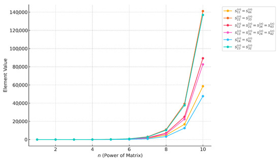
Figure 1. Growth trends of the matrix $S_4^n(2,1)$ for $1\le n\le 10$.

This experiment confirms the exponential nature of growth in matrix entries derived from Fibonacci-based closed forms. The plotted behavior also supports the theoretical results discussed in the manuscript.

Continuing from the pattern established in the previous example, we now examine the matrix $S_4^n(1,3)$ corresponding to the pair $(x,y)=(L_1,L_2)$. The resulting eigenvalues and associated sine product values are summarized in Table 2 and Table 4 and used to compute the matrix entries $s_{hk}^{\left(n\right)}\left(1,3\right)$.

Table 4. Eigenvalues of the matrix $S_4^n\left(1,3\right)$.

j	1	2	3	4
${\left(1+6cos\frac{j\pi }{5}\right)}^n$	${\left(\sqrt{5}{\alpha }^2\right)}^n$	${\left(\sqrt{5}-\beta \right)}^n$	${\left(-\sqrt{5}{\beta }^2\right)}^n$	${\left(-1\right)}^n{\left(\sqrt{5}+\alpha \right)}^n$

Theorem 2.

We let $F_n$ and $L_n$ represent the $n^{th}$ Fibonacci and Lucas numbers, respectively. The entries of the matrix $S_4^n(1,3)$ are expressed as

$$s_{1k}^{\left(n\right)}\left(1,3\right)={\displaystyle \frac{1}{2}}\left[5^{\lfloor \frac{n}{2}\rfloor }{W}_{2n-1}-{(-1)}^{n+k}{X}_{n-1}\right],k\in \{1,4\}$$

(14)

$$s_{1k}^{\left(n\right)}\left(1,3\right)={\displaystyle \frac{1}{2}}\left[5^{\lfloor \frac{n}{2}\rfloor }{W}_{2n}-{(-1)}^{n+k}{X}_n\right],k\in \{2,3\}$$

(15)

$$s_{3k}^{\left(n\right)}\left(1,3\right)={\displaystyle \frac{1}{2}}\left[5^{\lfloor \frac{n}{2}\rfloor }{W}_{2n+1}-{(-1)}^{n+k}{X}_{n+1}\right],k\in \{2,3\}$$

(16)

where the symbol $\lfloor x\rfloor$ is the greatest integer function for any real number x, $W_n$ stands for $L_n$ (n odd) or $F_n$ (n even), and we let

$$X_r=\sum _{t=0}^{\lfloor \frac{n}{2}\rfloor }{5}^t\left[\left({\displaystyle \genfrac{}{}{0pt}{}{n}{2t}}\right)F_{r-2t}+\left({\displaystyle \genfrac{}{}{0pt}{}{n}{2t+1}}\right)L_{r-2t-1}\right],$$

where the symbol $\left({\displaystyle \genfrac{}{}{0pt}{}{n}{t}}\right)$ is the binomial coefficient, $n\ge t\ge 0$, otherwise 0.

Proof. 

By using the values in Table 1 along with Equations (4)–(6), we construct Table 4.

According to Equation (8), the entries of the matrix $S_4^n\left(1,3\right)$ are expressed based on pairs $(h,k)=(1,2)$. By substituting values in the Table 2 and Table 4, we find

$$\begin{array}{ccc}\hfill s_{12}^{\left(n\right)}\left(1,3\right)& =& {\displaystyle \frac{1}{2\sqrt{5}}}\left[5^{n/2}\left({\alpha }^{2n}-{(-1)}^n{\beta }^{2n}\right)-{(-1)}^n\sum _{t=0}^n\left({\displaystyle \genfrac{}{}{0pt}{}{n}{t}}\right)5^{t/2}\left({\alpha }^{n-t}-{(-1)}^t{\beta }^{n-t}\right)\right]\hfill \end{array}$$

By using the Binet formulas for Fibonacci and Lucas numbers in Equation (1), and defining the auxiliary sum

$$X_r=\sum _{t=0}^{\lfloor \frac{n}{2}\rfloor }{5}^t\left[\left({\displaystyle \genfrac{}{}{0pt}{}{n}{2t}}\right)F_{r-2t}+\left({\displaystyle \genfrac{}{}{0pt}{}{n}{2t+1}}\right)L_{r-2t-1}\right],$$

we express the result in a more compact form. Additionally, we define

$$W_n=\left\{\begin{array}{cc}{L}_n,\hfill & \mathrm{if}n\mathrm{is}\mathrm{odd}\hfill \\ F_n,\hfill & \mathrm{if}n\mathrm{is}\mathrm{even}\hfill \end{array}\right.$$

Applying this structure to other entries and using the symmetry of $S_4^n\left(1,3\right)$, we obtain the remaining elements in (14)–(16). The derivation for each case follows similarly by choosing appropriate index pairs $(h,k)$ and applying the same expansion technique. □

In general, we investigate how the elements of the matrix $S_4^n(L_s,L_{s+1})$ relate to Fibonacci and Lucas numbers. Specifically, we derive closed-form expressions for its entries and demonstrate their dependence on $F_n$ and $L_n$.

Theorem 3.

We let $F_n$ and $L_n$ denote the $n^{th}$ Fibonacci and Lucas numbers, respectively. The entries of the matrix $S_4^n\left(L_s,L_{s+1}\right)$ are given as

$$s_{1k}^{\left(n\right)}\left(L_s,L_{s+1}\right)={\displaystyle \frac{1}{2}}\left[5^{\lfloor \frac{n}{2}\rfloor }{W}_{\left(s+1\right)n-1}-{(-1)}^{n+k}{X}_{n-1}\right],k\in \{1,4\}$$

(17)

$$s_{1k}^{\left(n\right)}\left(L_s,L_{s+1}\right)={\displaystyle \frac{1}{2}}\left[5^{\lfloor \frac{n}{2}\rfloor }{W}_{\left(s+1\right)n}-{(-1)}^{n+k}{X}_n\right],k\in \{2,3\}$$

(18)

$$s_{3k}^{\left(n\right)}\left(L_s,L_{s+1}\right)={\displaystyle \frac{1}{2}}\left[5^{\lfloor \frac{n}{2}\rfloor }{W}_{\left(s+1\right)n+1}-{(-1)}^{n+k}{X}_{n+1}\right],k\in \{2,3\}$$

(19)

where the symbol $\lfloor x\rfloor$ is the greatest integer function for any real number x and $W_n$ stands for $F_n$ (n even) or $L_n$ (n odd); we let

$$X_r=\sum _{t=0}^n\left({\displaystyle \genfrac{}{}{0pt}{}{n}{t}}\right){\left(-1\right)}^t{L}_s^t{L}_{s+1}^{n-t}{F}_{r-t},$$

(20)

where the symbol $\left({\displaystyle \genfrac{}{}{0pt}{}{n}{t}}\right)$ is the binomial coefficient, $n\ge t\ge 0$.

Proof. 

For the case $j=1$, by using the expressions in Equations (4)–(6) and Table 1, we obtain

$${\left(L_s+\alpha L_{s+1}\right)}^n={\left(\sqrt{5}{\alpha }^{s+1}\right)}^n.$$

Similar computations for $j=2,3,4$ yield the remaining eigenvalues, leading to the construction of Table 5.

Table 5. Eigenvalues of the matrix $S_4^n\left(L_s,L_{s+1}\right)$.

j	1	2	3	4
${\left(L_s+2L_{s+1}cos\frac{j\pi }{5}\right)}^n$	$5^{\frac{n}{2}}{\alpha }^{(s+1)n}$	${\left(L_s-\beta L_{s+1}\right)}^n$	$5^{\frac{n}{2}}{\left(-{\beta }^{(s+1)}\right)}^n$	${\left(L_s-\alpha L_{s+1}\right)}^n$

Substituting the corresponding values from Table 2 and Table 5 into Equation (8) for the entry $s_{11}^{\left(n\right)}\left(L_s,L_{s+1}\right)$, we obtain

$$\begin{array}{cc}\hfill s_{11}^{\left(n\right)}\left(L_s,L_{s+1}\right)& ={\displaystyle \frac{1}{2\sqrt{5}}}\left[5^{n/2}\left({\alpha }^{(s+1)n-1}-{(-1)}^n{\beta }^{(s+1)n-1}\right)+{\left(L_s-\beta L_{s+1}\right)}^n\alpha -{\left(L_s-\alpha L_{s+1}\right)}^n\beta \right]\hfill \end{array}$$

After simplification using Binet formulas in Equation (1), we obtain

$$s_{11}^{\left(n\right)}\left(L_s,L_{s+1}\right)=\left\{\begin{array}{cc}{\displaystyle \frac{1}{2}}\left[5^{\frac{n-1}{2}}{L}_{\left(s+1\right)n-1}-{\displaystyle \sum _{t=0}^n}\left({\displaystyle \genfrac{}{}{0pt}{}{n}{t}}\right){\left(-1\right)}^t{L}_s^t{L}_{s+1}^{n-t}{F}_{n-t-1}\right],\hfill & \mathrm{if} n \mathrm{is} \mathrm{odd} \hfill \\ {\displaystyle \frac{1}{2}}\left[5^{\frac{n}{2}}{F}_{\left(s+1\right)n-1}+{\displaystyle \sum _{t=0}^n}\left({\displaystyle \genfrac{}{}{0pt}{}{n}{t}}\right){\left(-1\right)}^t{L}_s^t{L}_{s+1}^{n-t}{F}_{n-t-1}\right],\hfill & \mathrm{if} n \mathrm{is} \mathrm{even}\hfill \end{array}\right.$$

Other elements not proven here are found similarly using appropriate values from the Table 2 and Table 5. □

Now, we include a comparative discussion to highlight the differences in complexity and combinatorial interpretation between the Fibonacci matrix $S_4^n(F_s,F_{s+1})$ in [16] and the Lucas matrix $S_4^n(L_s,L_{s+1})$. From a structural viewpoint, both matrix families share a binomial-based formulation, as shown in the appropriate theorems for Fibonacci matrices and its Lucas counterpart. However, notable distinctions arise in the nature of the sequences and the recursive dependencies involved.

In the Fibonacci case [16], the entries are expressed as linear combinations of Fibonacci numbers with coefficients derived from binomial terms involving powers of $F_{s+1}$ and $F_s$ and convolution with a shifted Fibonacci term:

$$s_{3k}^{\left(n\right)}(F_s,F_{s+1})={\displaystyle \frac{1}{2}}\left[F_{(s+1)n+1}-{(-1)}^k\sum _{t=0}^n\left({\displaystyle \genfrac{}{}{0pt}{}{n}{t}}\right){(-1)}^{n-t}{F}_s^t{F}_{s+1}^{n-t}{F}_{n-t+1}\right],k\in \{2,3\}.$$

This structure reflects a straightforward combinatorial construction based solely on the Fibonacci sequence.

In contrast, the Lucas case introduces additional complexity through two mechanisms.

Hybrid Fibonacci–Lucas Selection: The function $W_n$, defined such that $W_n=L_n$ for odd n, and $W_n=F_n$ for even n, introduces conditional behavior in the main term. This alternating dependency complicates both combinatorial interpretation and closed-form analysis, especially for large n.

Shifted Fibonacci Convolution with Lucas Coefficients: The auxiliary term $X_r$ given by

$$X_r=\sum _{t=0}^n\left({\displaystyle \genfrac{}{}{0pt}{}{n}{t}}\right){\left(-1\right)}^t{L}_s^t{L}_{s+1}^{n-t}{F}_{r-t}$$

combines Lucas sequence coefficients with Fibonacci indices. This convolution blends two distinct second-order linear recursions and requires the tracking of cross-sequence interactions over varying shifts $r-t$, leading to a more complex combinatorial representation.

Furthermore, in terms of computational complexity, the Fibonacci expressions grow polynomially in terms of the number of arithmetic operations with clear recurrence depth, while the Lucas matrix entries, due to the mixed-sequence summations and parity-conditioned behavior, involve additional branching and sequence evaluation, increasing the computational overhead. These differences underscore the richer structural and algebraic behavior encoded in the Lucas matrix formulation.

We present this comparative discussion specifically for the initial part of the study, as the structural patterns and combinatorial interpretations in subsequent sections follow similar principles. Therefore, a separate discussion section is not included. Nonetheless, we clearly articulate the generalizations and conclusions in each corresponding section of the manuscript.

In [21], Filipponi presented various sum and difference identities involving entries of the matrix $S_4^n(F_s,F_{s+1})$. Analogous examples can be constructed for the matrix $S_4^n(L_{s+1},L_s)$ based on its entries given in Equations (17)–(19). Now, the matrix $S_4^n(F_s,F_{s+1})$ is also expressed in terms of $S_4^n(L_0,L_1)$ and $S_4^n(L_1,L_2)$ as follows:

$$5^n{S}_4^n(F_s,F_{s+1})={\left[L_s{S}_4(1,3)+L_{s-1}{S}_4(2,1)\right]}^n$$

(21)

In addition, the matrix $S_4^n(L_s,L_{s+1})$ is expressed according to the matrices $S_4^n(F_0,F_1)$ and $S_4^n(F_1,F_2)$ given in [21] as follows:

$$\begin{array}{ccc}\hfill S_4^n(L_s,L_{s+1})& =& {\left[L_s{S}_4(1,1)+L_{s-1}{S}_4(0,1)\right]}^n,\hfill \end{array}$$

(22)

$$\begin{array}{ccc}\hfill & =& {\left[L_{s+1}{S}_4(1,1)-L_{s-1}{I}_4\right]}^n.\hfill \end{array}$$

(23)

These results provide a comprehensive understanding of the relationship between the matrix entries in Equations (17)–(19) and Fibonacci numbers within the context of the matrix $S_4^n(L_s,L_{s+1})$ as expressed in Equations (22) and (23). Specifically, we have

$$\begin{array}{cc}\hfill S_4^n(L_s,L_{s+1})& =\sum _{k=0}^n\left({\displaystyle \genfrac{}{}{0pt}{}{n}{k}}\right)L_s^k{L}_{s-1}^{n-k}{S}_4^k(1,1)S_4^{n-k}(0,1)\hfill \\ \hfill & =\sum _{k=0}^n\left({\displaystyle \genfrac{}{}{0pt}{}{n}{k}}\right){(-1)}^{n-k}{L}_{s+1}^k{L}_{s-1}^{n-k}{S}_4^k(1,1).\hfill \end{array}$$

Moreover, by applying the results in [7,21] together with Equations (21)–(23), one can derive various finite sum identities involving Fibonacci numbers. We leave these derivations to the interested reader.

2.2. Lucas Matrices Based on the Ordered Pair $(L_{s+1},L_s)$, $s\ge 0$

In this section, we first consider the special case $s=0$, with the ordered pair $(x,y)=(L_1,L_0)$, where $L_0=2$ and $L_1=1$. As noted in the study by Filipponi (1997) [21], the matrix $S_4^n(F_2,F_3)$ already coincides with this case and thus requires no modification. For the case $s=1$, we examine the ordered pair $(x,y)=(L_2,L_1)$, corresponding to the matrix $S_4^{\left(n\right)}(3,1)$.

Theorem 4.

We let $F_n$ and $L_n$ denote the $n^{th}$ Fibonacci and Lucas numbers, respectively. The entries of the matrix $S_4^n(3,1)$ are given by

$$s_{4k}^{\left(n\right)}(3,1)={\displaystyle \frac{1}{2}}\left[{(-1)}^k{5}^{\lfloor \frac{n}{2}\rfloor }{W}_{n+1}+X_{-1}\right],k\in \{1,4\}$$

(24)

$$s_{1k}^{\left(n\right)}(3,1)={\displaystyle \frac{1}{2}}\left[{(-1)}^k{5}^{\lfloor \frac{n}{2}\rfloor }{W}_n+X_0\right],k\in \{2,3\}$$

(25)

$$s_{2k}^{\left(n\right)}(3,1)={\displaystyle \frac{1}{2}}\left[{(-1)}^k{5}^{\lfloor \frac{n}{2}\rfloor }{W}_{n-1}+X_1\right],k\in \{2,3\}$$

(26)

where the symbol $\lfloor x\rfloor$ denotes the greatest integer less than or equal to a real number x, and where $W_n$ denotes $L_n$ if n is odd, and $F_n$ if n is even. The quantity $X_r$ is given by

$$X_r=\sum _{t=0}^{\lfloor \frac{n}{2}\rfloor }{5}^t\left[\left({\displaystyle \genfrac{}{}{0pt}{}{n}{2t}}\right)F_{2t+r}+\left({\displaystyle \genfrac{}{}{0pt}{}{n}{2t+1}}\right)L_{2t+r+1}\right],r\in \{-1,0,1\},$$

where $\left({\displaystyle \genfrac{}{}{0pt}{}{n}{t}}\right)$ is the binomial coefficient, defined for $n\ge t\ge 0$, and is zero otherwise.

Proof. 

For the matrix $S_4^n(3,1)$, using the expressions in Equations (4)–(6) and the values from Table 1, we obtain the eigenvalues listed in Table 6.

Table 6. Eigenvalues of the matrix $S_4^n(3,1)$.

j	1	2	3	4
${(3+2cos\frac{j\pi }{5})}^n$	${(1+\sqrt{5}\alpha )}^n$	${\left(\sqrt{5}\alpha \right)}^n$	${(1-\sqrt{5}\beta )}^n$	${(-\sqrt{5}\beta )}^n$

By substituting the corresponding values from Table 2 and Table 6 into Equation (8) for the pair $(h,k)=(4,4)$, the entry $s_{44}^{\left(n\right)}(3,1)$ is given by

$$\begin{array}{ccc}\hfill s_{44}^{\left(n\right)}(3,1)& =& {\displaystyle \frac{1}{2\sqrt{5}}}\left[5^{\frac{n}{2}}({\alpha }^{n+1}-{(-1)}^n{\beta }^{n+1})+\sum _{t=0}^n\left({\displaystyle \genfrac{}{}{0pt}{}{n}{t}}\right)5^{t/2}({\alpha }^{t-1}-{(-1)}^t{\beta }^{t-1})\right].\hfill \end{array}$$

By applying the Binet formulas in Equation (1), and considering the parity of n and t, the desired results follow. The proofs of Equations (24)–(26) are obtained by evaluating the corresponding matrix entries for each ordered pair $(h,k)$, using the values from Table 2 and Table 6 in conjunction with Equation (8). □

Finally, according to the ordered pair $(x,y)=(L_{s+1},L_s)$, we derive a closed-form expression for the entries of the matrix $S_4^n(L_{s+1},L_s)$.

Theorem 5.

We let $F_n$ and $L_n$ denote the $n^{th}$ Fibonacci and Lucas numbers, respectively. The entries of the matrix $S_4^n(L_{s+1},L_s)$ are

$$s_{1k}^{\left(n\right)}(L_{s+1},L_s)={\displaystyle \frac{1}{2}}\left[{(-1)}^k{5}^{\lfloor \frac{n}{2}\rfloor }{W}_{sn}+X_n\right],k\in \{2,3\}$$

(27)

$$s_{4k}^{\left(n\right)}(L_{s+1},L_s)={\displaystyle \frac{1}{2}}\left[{(-1)}^k{5}^{\lfloor \frac{n}{2}\rfloor }{W}_{sn+1}+X_{n-1}\right],k\in \{1,4\}$$

(28)

$$s_{2k}^{\left(n\right)}(L_{s+1},L_s)={\displaystyle \frac{1}{2}}\left[{(-1)}^k{5}^{\lfloor \frac{n}{2}\rfloor }{W}_{sn-1}+X_{n+1}\right],k\in \{2,3\}$$

(29)

where $\lfloor x\rfloor$ denotes the greatest integer less than or equal to x, $W_n=L_n$ if n is odd, and $W_n=F_n$ if n is even, and

$$X_r=\sum _{t=0}^n\left({\displaystyle \genfrac{}{}{0pt}{}{n}{t}}\right)L_{s+1}^t{L}_s^{n-t}{F}_{r-t},$$

with $\left({\displaystyle \genfrac{}{}{0pt}{}{n}{t}}\right)$ denoting the binomial coefficient, $n\ge t\ge 0$.

Proof. 

By employing the values from Table 1 together with Equations (4)–(6), we obtain the eigenvalues presented in Table 7.

Table 7. Eigenvalues of the matrix $S_4^{\left(n\right)}(L_{s+1},L_s)$.

j	1	2	3	4
${(L_{s+1}+2L_{s}cos\frac{j\pi }{5})}^n$	${(L_{s+1}+\alpha L_s)}^n$	$5^{n/2}{\alpha }^{sn}$	${(L_{s+1}+\beta L_s)}^n$	${(-1)}^n{5}^{n/2}{\beta }^{sn}$

For the pair $(h,k)=(2,2)$, substituting the corresponding values from Table 2 and Table 7 into Equation (8) yields

$$\begin{array}{cc}\hfill s_{22}^{\left(n\right)}(L_{s+1},L_s)& ={\displaystyle \frac{1}{2\sqrt{5}}}\left[5^{n/2}({\alpha }^{sn-1}-{(-1)}^n{\beta }^{sn-1})+\sum _{t=0}^n\left({\displaystyle \genfrac{}{}{0pt}{}{n}{t}}\right)L_{s+1}^t{L}_s^{n-t}({\alpha }^{n-t+1}-{\beta }^{n-t+1})\right]\hfill \end{array}$$

Considering whether n is odd or even, and applying the Binet formulas from Equation (1), we obtain

$$s_{22}^{\left(n\right)}(L_{s+1},L_s)=\left\{\begin{array}{cc}{\displaystyle \frac{1}{2}}\left[5^{(n-1)/2}{L}_{sn-1}+{\displaystyle \sum _{t=0}^n}\left({\displaystyle \genfrac{}{}{0pt}{}{n}{t}}\right)L_{s+1}^t{L}_s^{n-t}{F}_{n-t+1}\right],\hfill & \mathrm{if} n \mathrm{is} \mathrm{odd}\hfill \\ {\displaystyle \frac{1}{2}}\left[5^{n/2}{F}_{sn-1}+{\displaystyle \sum _{t=0}^n}\left({\displaystyle \genfrac{}{}{0pt}{}{n}{t}}\right)L_{s+1}^t{L}_s^{n-t}{F}_{n-t+1}\right],\hfill & \mathrm{if} n \mathrm{is} \mathrm{even}\hfill \end{array}\right.$$

The remaining entries given in Equations (27)–(29) can be derived analogously by substituting the relevant values from Table 2 and Table 7 into Equation (8). □

Moreover, the matrix $S_4^n(L_{s+1},L_s)$ can be expressed in terms of the matrices $S_4^n(0,1)$ and $S_4^n(1,1)$, as presented in [21], as follows:

$$\begin{array}{ccc}\hfill S_4^n(L_{s+1},L_s)& =& {\left[L_s{S}_4(1,1)+L_{s-1}{I}_4\right]}^n,\hfill \end{array}$$

(30)

$$\begin{array}{ccc}\hfill & =& {\left[L_{s+1}{S}_4(1,1)-L_{s-1}{S}_4^n(0,1)\right]}^n.\hfill \end{array}$$

(31)

These formulations provide a deeper understanding of the relationship between the matrix entries given in Equations (27)–(29) and the Fibonacci and Lucas numbers. In particular, the matrix $S_4^n(L_s,L_{s+1})$ can be expanded as

$$\begin{array}{cc}\hfill S_4^n(L_s,L_{s+1})& =\sum _{k=0}^n\left({\displaystyle \genfrac{}{}{0pt}{}{n}{k}}\right)L_s^k{L}_{s-1}^{n-k}{S}_4^k(1,1),\hfill \\ \hfill & =\sum _{k=0}^n\left({\displaystyle \genfrac{}{}{0pt}{}{n}{k}}\right){(-1)}^{n-k}{L}_{s+1}^k{L}_{s-1}^{n-k}{S}_4^k(1,1)S_4^{n-k}(0,1).\hfill \end{array}$$

Furthermore, the matrix $S_4^n(F_{s+1},F_s)$ can be represented in terms of $S_4^n(L_1,L_0)$ and $S_4^n(L_2,L_1)$ by identity

$$5^n{S}_4^n(F_{s+1},F_s)={\left[L_s{S}_4(3,1)+L_{s-1}{S}_4(1,2)\right]}^n.$$

2.3. Lucas Matrices Based on the Ordered Pair $(L_{-s},L_{-(s+1)})$, $s\ge 0$

In this subsection, we examine matrices $S_4(x,y)$ constructed using the ordered pair $(x,y)=(L_{-s},L_{-(s+1)})$, where $s\ge 0$. Although the parameter s is taken as non-negative for notational convenience, the subscripts $-s$ and $-(s+1)$ correspond to Lucas numbers with negative indices. This formulation allows us to systematically analyze cases involving negative-indexed terms while maintaining consistency with the structure of the previous sections. In the special case where $s=0$, corresponding to the ordered pair $(L_0,L_{-1})=(2,-1)$, the matrix $S_4^n(2,-1)$ takes the following form:

Theorem 6.

We let $F_n$ and $L_n$ denote the $n^{th}$ Fibonacci and Lucas numbers, respectively. Then, the entries of the matrix $S_4^n(L_0,L_{-1})$ are given by

$$s_{4k}^{\left(n\right)}\left(2,-1\right)={\displaystyle \frac{1}{2}}\left[F_{2n+1}+{(-1)}^k{5}^{⌊n/2⌋}{W}_{n-1}\right],k\in \{1,4\}$$

(32)

$$s_{4k}^{\left(n\right)}\left(2,-1\right)={\displaystyle \frac{1}{2}}\left[-F_{2n}+{(-1)}^k{5}^{⌊n/2⌋}{W}_n\right],k\in \{2,3\}$$

(33)

$$s_{2k}^{\left(n\right)}\left(2,-1\right)={\displaystyle \frac{1}{2}}\left[F_{2n-1}+{(-1)}^k{5}^{⌊n/2⌋}{W}_{n+1}\right],k\in \{2,3\}$$

(34)

where $\lfloor x\rfloor$ denotes the greatest integer less than or equal to x and $W_n$ stands for $F_n$ (n even) or $L_n$ (n odd).

Proof. 

To derive the results presented in Table 8 for the matrix $S_4^n(2,-1)$, we utilize the identities given in Equations (4)–(6) together with the values listed in Table 1.

Table 8. Eigenvalues of the matrix $S_4^n\left(2,-1\right)$.

j	1	2	3	4
${\left(2-2cos\frac{j\pi }{5}\right)}^n$	${\beta }^{2n}$	${\left(-\sqrt{5}\beta \right)}^n$	${\alpha }^{2n}$	${\left(\sqrt{5}\alpha \right)}^n$

If appropriate values from Table 2 and Table 8 are substituted into Equation (8) for $(h,k)=(4,3)$, we obtain

$$\begin{array}{ccc}\hfill s_{43}^{\left(n\right)}\left(2,-1\right)& =& {\displaystyle \frac{1}{2}}\left[-{\displaystyle \frac{{\alpha }^{2n}-{\beta }^{2n}}{\sqrt{5}}}-5^{\left(n-1\right)/2}\left({\alpha }^n-{\left(-1\right)}^n{\beta }^n\right)\right].\hfill \end{array}$$

From the Binet formula in Equation (1) depending on whether n is odd or even, we find

$$s_{43}^{\left(n\right)}\left(2,-1\right)=\left\{\begin{array}{cc}{\displaystyle \frac{1}{2}}\left(-F_{2n}-5^{\frac{n-1}{2}}{L}_n\right),\hfill & n \mathrm{is} \mathrm{odd}\hfill \\ {\displaystyle \frac{1}{2}}\left(-F_{2n}-5^{\frac{n}{2}}{F}_n\right),\hfill & n \mathrm{is} \mathrm{even}\hfill \end{array}\right..$$

By substituting the appropriate values of the ordered pair $(h,k)$ from Table 2 and Table 8 into Equation (8), we obtain the remaining entries and thereby complete the proof of Equations (32)–(34). □

In the special case where $s=1$, the ordered pair becomes $(L_{-1},L_{-2})=(-1,3)$, and the matrix $S_4^n(-1,3)$ takes the following form:

Theorem 7.

We let $F_n$ and $L_n$ denote the $n^{th}$ Fibonacci and Lucas numbers, respectively. Then, the entries of the matrix $S_4^n(-1,3)$ are given by

$$s_{4k}^{\left(n\right)}(-1,3)={\displaystyle \frac{1}{2}}\left[{(-1)}^{n+k}{5}^{\lfloor \frac{n}{2}\rfloor }{W}_{2n-1}+X_{n-1}\right],k\in \{1,4\}$$

(35)

$$s_{2k}^{\left(n\right)}(-1,3)={\displaystyle \frac{1}{2}}\left[{(-1)}^{n+k}{5}^{\lfloor \frac{n}{2}\rfloor }{W}_{2n}+X_n\right],k\in \{1,4\}$$

(36)

$$s_{2k}^{\left(n\right)}(-1,3)={\displaystyle \frac{1}{2}}\left[{(-1)}^{n+k}{5}^{\lfloor \frac{n}{2}\rfloor }{W}_{2n+1}+X_{n+1}\right],k\in \{2,3\}$$

(37)

where the symbol $⌊x⌋$ denotes the floor function (i.e., the greatest integer less than or equal to x) and the symbol $W_n$ denotes the Lucas number $L_n$ when n is odd, and the Fibonacci number $F_n$ when n is even, and

$$X_r=\sum _{t=0}^{\lfloor \frac{n}{2}\rfloor }{5}^t\left[\left({\displaystyle \genfrac{}{}{0pt}{}{n}{2t}}\right)F_{r-2t}+\left({\displaystyle \genfrac{}{}{0pt}{}{n}{2t+1}}\right)L_{r-2t-1}\right],$$

with $\left({\displaystyle \genfrac{}{}{0pt}{}{n}{t}}\right)$ representing the binomial coefficient, where $n\ge t\ge 0$ (and zero otherwise).

Proof. 

Using the matrix $S_4^{\left(n\right)}(-1,3)$ along with the identities in Equations (4)–(6) and the eigenvalues listed in Table 9, we derive the stated results.

Table 9. Eigenvalues of the matrix $S_4^{\left(n\right)}(-1,3)$.

j	1	2	3	4
${(-1+6cos\left(\frac{j\pi }{5}\right))}^n$	${(\alpha +\sqrt{5})}^n$	${\left(\sqrt{5}{\beta }^2\right)}^n$	${(\beta -\sqrt{5})}^n$	${(-\sqrt{5}{\alpha }^2)}^n$

Substituting the relevant values from Table 2 and Table 9 into Equation (8) for the entry with $(h,k)=(1,1)$, we obtain

$$\begin{array}{cc}\hfill s_{11}^{\left(n\right)}(-1,3)& ={\displaystyle \frac{1}{2\sqrt{5}}}\left[5^{n/2}\left({(-1)}^n{\alpha }^{2(n-1)}-{\beta }^{2(n-1)}\right)+\sum _{t=0}^n\left({\displaystyle \genfrac{}{}{0pt}{}{n}{t}}\right)5^{t/2}\left({\alpha }^{n-t-1}-{(-1)}^t{\beta }^{n-t-1}\right)\right]\hfill \end{array}$$

By applying Binet formulas in Equation (1) and considering the parity of n, we deduce

$$s_{11}^{\left(n\right)}(-1,3)=\left\{\begin{array}{cc}{\displaystyle \frac{1}{2}}\left[-5^{(n-1)/2}{L}_{2n-1}+{\displaystyle \sum _{t=0}^{(n-1)/2}}{5}^t\left(\left({\displaystyle \genfrac{}{}{0pt}{}{n}{2t}}\right)F_{n-2t-1}+\left({\displaystyle \genfrac{}{}{0pt}{}{n}{2t+1}}\right)L_{n-2t-2}\right)\right],\hfill & \mathrm{if} n \mathrm{is} \mathrm{odd}\hfill \\ {\displaystyle \frac{1}{2}}\left[5^{n/2}{F}_{2n-1}+F_{n-1}+{\displaystyle \sum _{t=1}^{n/2}}\left(\left({\displaystyle \genfrac{}{}{0pt}{}{n}{2t}}\right)5^t{F}_{n-2t-1}+\left({\displaystyle \genfrac{}{}{0pt}{}{n}{2t-1}}\right)5^{t-1}{L}_{n-2t}\right)\right],\hfill & \mathrm{if} n \mathrm{is} \mathrm{even}\hfill \end{array}\right.$$

The proofs of the other entries in Equations (35)–(37) follow from similar arguments, by substituting the corresponding values for $(h,k)$ from Table 2 and Table 9 into Equation (8). □

Considering the identity for Lucas numbers with negative indices given in Equation (2), we have $L_{-s}={(-1)}^s{L}_s\mathrm{and}{L}_{-(s+1)}=-{(-1)}^s{L}_{s+1},s\ge 0$. Using these identities, if we define the matrix entries with the pair $(x,y)=(L_{-s},L_{-(s+1)})$, then the following relation holds:

$$S_4^n(L_{-s},L_{-(s+1)})={(-1)}^{sn}{S}_4^n(L_s,-L_{s+1}),s\ge 0.$$

Theorem 8.

We let $F_n$ and $L_n$ denote the $n^{th}$ Fibonacci and Lucas numbers, respectively. Then the entries of the matrix $S_4^n(L_{-s},L_{-(s+1)})$ are given by

$$s_{2k}^{\left(n\right)}(L_{-s},L_{-(s+1)})={\displaystyle \frac{{(-1)}^{sn}}{2}}\left[5^{\lfloor \frac{n}{2}\rfloor }{W}_{(s+1)n}+{(-1)}^n{X}_n\right],k\in \{1,4\}$$

(38)

$$s_{4k}^{\left(n\right)}(L_{-s},L_{-(s+1)})={\displaystyle \frac{{(-1)}^{sn}}{2}}\left[{(-1)}^k{5}^{\lfloor \frac{n}{2}\rfloor }{W}_{(s+1)n-1}+{(-1)}^n{X}_{n-1}\right],k\in \{1,4\},$$

(39)

$$s_{2k}^{\left(n\right)}(L_{-s},L_{-(s+1)})={\displaystyle \frac{{(-1)}^{sn}}{2}}\left[{(-1)}^k{5}^{\lfloor \frac{n}{2}\rfloor }{W}_{(s+1)n+1}+{(-1)}^n{X}_{n+1}\right],k\in \{2,3\}$$

(40)

where $\lfloor x\rfloor$ denotes the greatest integer less than or equal to x, $W_n=L_n$ if n is odd, and $W_n=F_n$ if n is even. Additionally, the function $X_r$ is given by

$$X_r=\sum _{t=0}^n\left({\displaystyle \genfrac{}{}{0pt}{}{n}{t}}\right){(-1)}^t{L}_s^t{L}_{s+1}^{n-t}{F}_{r-t}$$

where $\left({\displaystyle \genfrac{}{}{0pt}{}{n}{t}}\right)$ denotes the binomial coefficient and is taken to be zero for $t>n$ or $t<0$.

Proof. 

Using the identities given in Equations (4)–(6), along with the values provided in Table 1, we compute the eigenvalues of the matrix $S_4^n(L_{-s},L_{-(s+1)})$ as shown in Table 10.

Table 10. Eigenvalues of the matrix $S_4^n(L_{-s},L_{-(s+1)})$.

j	1	2	3	4
${(L_s-2L_{s+1}cos\frac{j\pi }{5})}^n$	${(L_s-\alpha L_{s+1})}^n$	$5^{n/2}{(-1)}^n{\left(\beta \right)}^{(s+1)n}$	${(L_s-\beta L_{s+1})}^n$	$5^{n/2}{\alpha }^{(s+1)n}$

By substituting the eigenvalue expressions from Table 2 and Table 10 into Equation (8) for the position $(h,k)=(1,3)$, we obtain

$$\begin{array}{cc}\hfill s_{13}^{\left(n\right)}(L_{-s},L_{-(s+1)})& ={\displaystyle \frac{{(-1)}^{sn}}{2\sqrt{5}}}[5^{n/2}({\alpha }^{(s+1)n}-{(-1)}^n{\beta }^{(s+1)n})\hfill \\ & +\sum _{t=0}^n\left({\displaystyle \genfrac{}{}{0pt}{}{n}{t}}\right){(-1)}^{n-t}{L}_s^t{L}_{s+1}^{n-t}({\alpha }^{n-t}-{\beta }^{n-t})]\hfill \end{array}$$

Applying the Binet formulas from Equation (1) and simplifying based on the parity of n, we deduce

$$s_{13}^{\left(n\right)}(L_{-s},L_{-(s+1)})=\left\{\begin{array}{cc}{\displaystyle \frac{{(-1)}^{sn}}{2}}\left[5^{(n-1)/2}{L}_{(s+1)n}-{\displaystyle \sum _{t=0}^n}\left({\displaystyle \genfrac{}{}{0pt}{}{n}{t}}\right){(-1)}^t{L}_s^t{L}_{s+1}^{n-t}{F}_{n-t}\right],\hfill & \mathrm{if} n \mathrm{is} \mathrm{odd}\hfill \\ {\displaystyle \frac{{(-1)}^{sn}}{2}}\left[5^{n/2}{F}_{(s+1)n}+{\displaystyle \sum _{t=0}^n}\left({\displaystyle \genfrac{}{}{0pt}{}{n}{t}}\right){(-1)}^t{L}_s^t{L}_{s+1}^{n-t}{F}_{n-t}\right],\hfill & \mathrm{if} n \mathrm{is} \mathrm{even}\hfill \end{array}\right.$$

The remaining matrix entries in Equations (38)–(40) follow similarly by substituting the corresponding eigenvalues from Table 2 and Table 10 into Equation (8). □

Extending our analysis to the matrices $S_4^n\left(L_{-s},L_{-(s+1)}\right)$ formed by negative-indexed Lucas numbers, we present new expressions involving matrix entries related to $S_4(F_0,F_{-1})$ and $S_4(F_{-1},F_{-2})$ (or equivalently $S_4(F_{-2},F_{-1})$), as previously discussed in [16]. Specifically, we obtain the following identities:

$$\begin{array}{cc}\hfill S_4^n\left(L_{-s},L_{-(s+1)}\right)& ={(-1)}^{sn}{\left[L_{s+1}{S}_4(F_{-1},F_{-2})-L_{s-1}{I}_4\right]}^n,s>0,\hfill \end{array}$$

(41)

$$\begin{array}{cc}\hfill & ={(-1)}^{sn}{\left[L_s{S}_4(F_{-1},F_{-2})-L_{s-1}{S}_4(F_0,F_{-1})\right]}^n,\hfill \end{array}$$

(42)

$$\begin{array}{cc}\hfill & ={(-1)}^{sn+1}{\left[L_s{S}_4(F_{-2},F_{-1})+L_{s-1}{S}_4(F_0,F_{-1})\right]}^n.\hfill \end{array}$$

(43)

These representations provide new insights into the structure of the matrix $S_4^n(L_{-s},L_{-(s+1)})$, revealing further algebraic and combinatorial properties inherent in the Fibonacci matrix framework.

Moreover, as shown in [16], the matrix $S_4^n(F_{-s},F_{-(s+1)})$ can be expressed in terms of $S_4^n(L_0,L_{-1})$ and $S_4^n(L_{-1},L_{-2})$ as follows:

$${(-1)}^{sn}{5}^n{S}_4^n(F_{-s},F_{-(s+1)})={\left[L_s{S}_4(-1,3)-L_{s-1}{S}_4(2,-1)\right]}^n,s>0.$$

(44)

These identities deepen our understanding of the Fibonacci and Lucas numbers interplay in the structure of powers of tridiagonal matrices.

2.4. Lucas Matrices Based on the Ordered Pair $\left(L_{-(s+1)},L_{-s}\right)$ for $s\ge 0$

In this part, we consider the matrices defined by the ordered pair $(x,y)=(L_{-(s+1)},L_{-s})$, where $s\ge 0$ and thus both subscripts are negative. This case complements the previous subsection by reversing the order of the components, further enriching the analysis of matrices constructed from negatively indexed Lucas numbers. For the case $s=0$, the identity $(L_{-1},L_0)=(-1,2)$, which follows from Equation (2), allows us to explicitly compute the powers of the matrix $S_4^n(-1,2)$.

Theorem 9.

We let $F_n$ denote the $n^{th}$ Fibonacci number. Then, the entries of the matrix $S_4^n(L_{-1},L_0)=S_4^n(-1,2)$ are given by

$$s_{1k}^{\left(n\right)}\left(-1,2\right)={\displaystyle \frac{1}{2}}\left({(-1)}^{n+k+1}{F}_{3n-1}+{\left(-1\right)}^n{5}^{⌊n/2⌋}\right),k\in \{1,4\}$$

(45)

$$s_{1k}^{\left(n\right)}\left(-1,2\right)={\displaystyle \frac{1}{2}}\left({\left(-1\right)}^{n+k+1}{F}_{3n}+5^{\left(n-1\right)/2}\left(1-{\left(-1\right)}^n\right)\right),k\in \{2,3\}$$

(46)

$$s_{23}^{\left(n\right)}\left(-1,2\right)={\displaystyle \frac{1}{2}}\left({\left(-1\right)}^{n+k}{F}_{3n+1}+5^{⌊n/2⌋}\right),k\in \{2,3\}$$

(47)

where $⌊x⌋$ denotes the greatest integer less than or equal to x, for any real number x.

Proof. 

Using the identities provided in Equations (4)–(6) and the values in Table 1, we have the eigenvalue powers presented in Table 11

Table 11. Eigenvalues of the matrix $S_4^n\left(-1,2\right)$.

j	1	2	3	4
${\left(-1+4cos\frac{j\pi }{5}\right)}^n$	$5^{n/2}$	${(-1)}^n{\beta }^{3n}$	${(-1)}^n{5}^{n/2}$	${(-1)}^n{\alpha }^{3n}$

Substituting the relevant values from Table 2 and Table 11 into Equation (8) for the pair $(h,k)=(1,3)$, we obtain

$$\begin{array}{ccc}\hfill s_{13}^{\left(n\right)}\left(-1,2\right)& =& {\displaystyle \frac{1}{2\sqrt{5}}}\left[{\left(-1\right)}^n\left({\alpha }^{3n}-{\beta }^{3n}\right)+5^{n/2}\left(1-{\left(-1\right)}^n\right)\right].\hfill \end{array}$$

The desired closed-form expression follows by applying the Binet formula from Equation (1). Similarly, by evaluating Equation (8) for the ordered pairs $(h,k)$ using the eigenvalues in Table 2 and Table 11, the remaining identities are established. □

For the ordered pair $(x,y)=(L_{-2},L_{-1})$, the matrix $S_4^n(3,-1)$ is given.

Theorem 10.

We let $F_n$ and $L_n$ denote the $n^{th}$ Fibonacci and Lucas numbers, respectively. The elements of the matrix $S_4^n(3,-1)$, corresponding to the ordered pair $(x,y)=(L_{-2},L_{-1})$, are given by

$$s_{4k}^{\left(n\right)}(3,-1)={\displaystyle \frac{1}{2}}\left[-5^{⌊n/2⌋}{W}_{n+1}+{(-1)}^k{X}_{-1}\right],k\in \{1,4\}$$

(48)

$$s_{4k}^{\left(n\right)}(3,-1)={\displaystyle \frac{1}{2}}\left[-5^{⌊n/2⌋}{W}_n+{(-1)}^k{X}_0\right],k\in \{2,3\}$$

(49)

$$s_{2k}^{\left(n\right)}(3,-1)={\displaystyle \frac{1}{2}}\left[-5^{⌊n/2⌋}{W}_{n-1}+{(-1)}^k{X}_1\right],k\in \{2,3\}$$

(50)

where the symbol $\lfloor x\rfloor$ is the greatest integer function for any real number x, where the symbol $⌊x⌋$ denotes the greatest integer less than or equal to x, $W_n$ stands for $L_n$ (n odd) or $F_n$ (n even), and

$$X_r=\sum _{t=0}^{⌊n/2⌋}{5}^t\left(\left({\displaystyle \genfrac{}{}{0pt}{}{n}{2t}}\right)F_{2t+r}+\left({\displaystyle \genfrac{}{}{0pt}{}{n}{2t+1}}\right)L_{2t+r+1}\right),r\in \{-1,0,1\},$$

where the symbol $\left({\displaystyle \genfrac{}{}{0pt}{}{n}{t}}\right)$ is the binomial coefficient, $n\ge t\ge 0$, otherwise 0.

Proof. 

To determine the entries of the matrix $S_4^n(3,-1)$, we utilize Equations (4)–(6) along with the values from Table 1. The relevant eigenvalues of the matrix $S_4^n\left(3,-1\right)$ are organized in Table 12.

Table 12. Eigenvalues of the matrix $S_4^n\left(3,-1\right)$.

j	1	2	3	4
${\left(3-2cos\frac{j\pi }{5}\right)}^n$	${(-1)}^n{5}^{n/2}{\beta }^n$	${(1-\sqrt{5}\beta )}^n$	$5^{n/2}{\alpha }^n$	${(1+\sqrt{5}\alpha )}^n$

To derive the element $s_{41}^{\left(n\right)}(3,-1)$ corresponding to the index pair $(h,k)=(4,1)$, we substitute the relevant values from Table 2 and Table 12 into Equation (8):

$$\begin{array}{cc}\hfill s_{41}^{\left(n\right)}(3,-1)& ={\displaystyle \frac{1}{2\sqrt{5}}}\left[5^{n/2}\left({\alpha }^{n+1}-{(-1)}^n{\beta }^{n+1}\right)-\sum _{t=0}^n\left({\displaystyle \genfrac{}{}{0pt}{}{n}{t}}\right)5^{t/2}\left({\alpha }^{t-1}-{(-1)}^t{\beta }^{t-1}\right)\right].\hfill \end{array}$$

By analyzing the parity of n and t and applying the Binet formulas in Equation (1), we obtain

$$s_{41}^{\left(n\right)}(3,-1)=\left\{\begin{array}{cc}{\displaystyle \frac{1}{2}}\left(5^{(n-1)/2}{L}_{n+1}-\sum _{t=0}^{\frac{n-1}{2}}{5}^t\left(\left({\displaystyle \genfrac{}{}{0pt}{}{n}{2t}}\right)F_{2t-1}+\left({\displaystyle \genfrac{}{}{0pt}{}{n}{2t+1}}\right)L_{2t}\right)\right),\hfill & \mathrm{if} n \mathrm{is} \mathrm{odd},\hfill \\ {\displaystyle \frac{1}{2}}\left(5^{n/2}{F}_{n+1}-1-\sum _{t=1}^{\frac{n}{2}}\left(\left({\displaystyle \genfrac{}{}{0pt}{}{n}{2t}}\right)5^t{F}_{2t-1}+\left({\displaystyle \genfrac{}{}{0pt}{}{n}{2t-1}}\right)5^{t-1}{L}_{2t-2}\right)\right),\hfill & \mathrm{if} n \mathrm{is} \mathrm{even}.\hfill \end{array}\right.$$

The derivations for the remaining matrix entries follow analogously by substituting the corresponding values from Table 2 and Table 12 into Equation (8). □

To extend these formulations by using the expressions in Equation (2), $L_{-s}={(-1)}^s{L}_s$, $s\ge 0,$ as shown in Equation (8) for the ordered pair elements $\left(x,y\right)=\left(L_{-(s+1)},L_{-s}\right)$, where $s>0$, the matrix $S_4^n\left(L_{-(s+1)},L_{-s}\right)$ is expressed as follows:

Theorem 11.

We let $F_n$ and $L_n$ denote the $n^{th}$ Fibonacci and Lucas numbers, respectively. The entries of the matrix $S_4^n(L_{-(s+1)},L_{-s})$ are given by

$$s_{2k}^{\left(n\right)}(L_{-(s+1)},L_{-s})={\displaystyle \frac{{(-1)}^{(s+1)n}}{2}}\left[-5^{\lfloor n/2\rfloor }{W}_{sn}+{(-1)}^k{X}_n\right],k\in \{1,4\}$$

(51)

$$s_{2k}^{\left(n\right)}(L_{-(s+1)},L_{-s})={\displaystyle \frac{{(-1)}^{(s+1)n}}{2}}\left[5^{\lfloor n/2\rfloor }{W}_{sn-1}+{(-1)}^k{X}_{n+1}\right],k\in \{2,3\}$$

(52)

$$s_{4k}^{\left(n\right)}(L_{-(s+1)},L_{-s})={\displaystyle \frac{{(-1)}^{(s+1)n}}{2}}\left[5^{\lfloor n/2\rfloor }{W}_{sn+1}+{(-1)}^k{X}_{n-1}\right],k\in \{1,4\}$$

(53)

where $\lfloor x\rfloor$ denotes the greatest integer less than or equal to x, $W_n$ is defined as $L_n$ if n is odd and $F_n$ if n is even, and

$$X_r=\sum _{t=0}^n\left({\displaystyle \genfrac{}{}{0pt}{}{n}{t}}\right)L_{s+1}^t{L}_s^{n-t}{F}_{r-t}$$

where the symbol $\left({\displaystyle \genfrac{}{}{0pt}{}{n}{t}}\right)$ is the binomial coefficient, $n\ge t\ge 0$, otherwise 0.

Proof. 

By applying Table 1 and Table 2 together with Equations (4)–(6), for the pair $(x,y)=(L_{-(s+1)},L_{-s})$, we obtain the eigenvalues listed in Table 13.

Table 13. Eigenvalues of the matrix $S_4^n(L_{-(s+1)},L_{-s})$.

j	1	2	3	4
${(-L_{s+1}+2L_{s}cos\frac{j\pi }{5})}^n$	$5^{n/2}{\beta }^{sn}$	${(-1)}^n{(L_{s+1}+\beta L_s)}^n$	${(-1)}^n{5}^{n/2}{\alpha }^{sn}$	${(-1)}^n{(L_{s+1}+\alpha L_s)}^n$

If the values from Table 2 and Table 13 are substituted into Equation (8) for $s_{21}^{\left(n\right)}(L_{-(s+1)},L_{-s})$, we obtain

$$\begin{array}{cc}\hfill s_{21}^{\left(n\right)}(L_{-(s+1)},L_{-s})& ={\displaystyle \frac{{(-1)}^{(s+1)n}}{2\sqrt{5}}}\left[-5^{n/2}({\alpha }^{sn}-{(-1)}^n{\beta }^{sn})-\sum _{t=0}^n\left({\displaystyle \genfrac{}{}{0pt}{}{n}{t}}\right)L_{s+1}^t{L}_s^{n-t}({\alpha }^{n-t}-{\beta }^{n-t})\right]\hfill \end{array}$$

Depending on the parity of n and using Equation (1), we obtain

$$s_{21}^{\left(n\right)}(L_{-(s+1)},L_{-s})=\left\{\begin{array}{cc}{\displaystyle \frac{{(-1)}^{(s+1)n}}{2}}\left[-5^{(n-1)/2}{L}_{sn}-{\displaystyle \sum _{t=0}^n}\left({\displaystyle \genfrac{}{}{0pt}{}{n}{t}}\right)L_{s+1}^t{L}_s^{n-t}{F}_{n-t}\right],\hfill & \mathrm{if} n \mathrm{is} \mathrm{odd}\hfill \\ {\displaystyle \frac{{(-1)}^{(s+1)n}}{2}}\left[-5^{n/2}{F}_{sn}-{\displaystyle \sum _{t=0}^n}\left({\displaystyle \genfrac{}{}{0pt}{}{n}{t}}\right){(-1)}^t{L}_{s+1}^t{L}_s^{n-t}{F}_{n-t}\right],\hfill & \mathrm{if} n \mathrm{is} \mathrm{even}\hfill \end{array}\right.$$

The remaining entries can be derived analogously by applying similar computations using the corresponding values from Table 2 and Table 13. □

Extending our analysis to the matrices $S_4^n\left(L_{-(s+1)},L_{-s}\right)$ formed by negatively indexed Lucas numbers, we derive expressions involving the entries of $S_4\left(F_{-1},F_0\right)$ and $S_4\left(F_{-2},F_{-1}\right)$ (or $S_4\left(F_{-1},F_{-2}\right)$) as presented in Koken and Aksoy [16]:

$$\begin{array}{ccc}\hfill S_4^n\left(L_{-(s+1)},L_{-s}\right)& =& {\left(-1\right)}^{sn}{\left[L_s{S}_4\left(F_{-2},F_{-1}\right)-L_{s-1}{S}_4\left(F_{-1},F_0\right)\right]}^n,s>0\hfill \\ & =& {\left(-1\right)}^{sn}{\left[L_{s+1}{S}_4\left(F_{-2},F_{-1}\right)-L_{s-1}{S}_4\left(F_0,F_{-1}\right)\right]}^n\hfill \\ & =& {\left(-1\right)}^{sn+1}{\left[L_{s+1}{S}_4\left(F_{-1},F_{-2}\right)+L_{s-1}{S}_4\left(F_0,F_{-1}\right)\right]}^n\hfill \\ & =& {\left(-1\right)}^{sn+1}{\left[L_s{S}_4\left(F_{-1},F_{-2}\right)+L_{s-1}{S}_4\left(F_{-1},F_0\right)\right]}^n.\hfill \end{array}$$

This progression facilitates the derivation of novel representations for the matrix $S_4^n\left(L_{-(s+1)},L_{-s}\right)$, offering deeper insights into the algebraic and combinatorial structures inherent in the Fibonacci matrix framework.

Moreover, the matrix $S_4^n\left(F_{-(s+1)},F_{-s}\right)$, as introduced in Koken and Aksoy [16], can be expressed in terms of $S_4^n(L_{-1},L_0)$ and $S_4^n(L_{-2},L_{-1})$ by the following identity:

$${(-1)}^{sn}{5}^n{S}_4^n\left(F_{-(s+1)},F_{-s}\right)={\left[L_s{S}_4(3,-1)-L_{s-1}{S}_4(-1,2)\right]}^n.$$

3. Discussion and Recommendation

The findings presented in this study, particularly the closed-form expressions derived for the powers of the matrix $S_4^n(x,y)$ in Section 2.1, Section 2.2, Section 2.3 and Section 2.4, provide significant insight into the algebraic structure of these matrices when x and y are selected as consecutive or symmetric Lucas numbers.

Special emphasis was placed on pairs satisfying the coprimality condition $\gcd (x,y)=1$ in order to explore the implications of such algebraic relationships in matrix constructions. Several avenues for future research were identified. These include extending the study to matrices defined by other coprime pairs such as $(F_s,F_{s+2})$, $(L_s,L_{s+2})$, and $(F_s,L_s)$, as well as deriving general expressions for the entries of $S_4^n(x,y)$ matrices based on these pairs. Further investigations could also focus on summation and difference identities derived from the closed-form expressions, as well as an examination of these results using matrix norms and algebraic operations.

An additional promising direction involves analyzing the behavior of the matrices $S_m(x,y)$ under advanced matrix operations such as the Hadamard, Kronecker, Khatri–Rao, and Tracy–Singh products. These algebraic constructions may reveal novel identities and uncover intricate relationships between Lucas and Fibonacci matrices. Such investigations could deepen our understanding of their underlying algebraic and spectral structures, possibly leading to broader generalizations and new combinatorial interpretations.

The theoretical developments established in this work provide a foundational framework for both pure and applied mathematical research. The matrix family $S_m(x,y)$, characterized by its tridiagonal symmetric structure and recursive Lucas-based entries, exhibits a rich algebraic form that invites further exploration. The closed-form expressions and recurrence behaviors identified herein offer a starting point for extending this framework to larger matrix dimensions or alternative recursive sequences.

From an applied perspective, Lucas-based tridiagonal matrices such as those studied in this paper arise naturally in various domains of discrete mathematics. In combinatorics, for instance, the number of ways to tile a $1\times n$ board using a combination of unit squares and $1\times 2$ dominoes—with tiling weights governed by Lucas-type recursions—can be encoded via the powers of a suitably defined $S_m(x,y)$ matrix. The matrix parameters reflect the recursive structure of the Lucas sequence, allowing for elegant representations of tiling configurations through matrix exponentiation.

In network theory, the matrix $S_m(x,y)$ may serve as the adjacency or Laplacian matrix of a path or cycle graph with m vertices, where edge weights evolve according to a Lucas sequence. In such settings, the spectral properties of $S_m(x,y)$ influence fundamental network behaviors, including diffusion dynamics, signal propagation, and stability conditions. The recursive nature of the weights introduces a structured complexity that may yield insights into the design and analysis of weighted networks with deterministic, number-theoretic constraints.

Overall, the results presented in this study highlight the versatility and depth of Lucas-based matrix families. Future research can focus on generalizing these structures to broader matrix classes and exploring their implications across discrete models, algebraic combinatorics, and spectral graph theory.

4. Conclusions

This study introduced a method for determining the values of x and y for which the matrix $S_4^n(x,y)$, constructed from the ordered pair $(x,y)$ with x and y being Lucas numbers, can be characterized as a Lucas matrix in a generalized framework.

In Section 2.1, Section 2.2, Section 2.3 and Section 2.4, we derived closed-form expressions for both specific and generalized entries of the matrix $S_4^n(x,y)$, corresponding to various ordered pairs, including $(x,y)=(L_s,L_{s+1})$, $(x,y)=(L_{s+1},L_s)$, $(x,y)=(L_{-s},L_{-(s+1)})$, and $(x,y)=(L_{-(s+1)},L_{-s})$.

In addition to the theoretical contributions discussed, this study briefly touched upon potential application areas of the proposed matrices $S_4^n(x,y)$. While these applications were mentioned to illustrate the broader relevance of the work, a more detailed exploration was intentionally deferred to future studies. The primary objective of this paper was to establish the algebraic structure and spectral properties of the matrices $S_4^n(x,y)$, particularly when constructed from coprime pairs of Lucas numbers.

The results presented in this paper establish a robust algebraic framework for the study of Lucas-based matrix structures and their closed-form behaviors. We expect that subsequent research will leverage this framework to advance both the theoretical development and practical deployment of such matrices in domains including coding theory, signal processing, and combinatorial optimization.

References

- Debnath, L. A short history of the Fibonacci and golden numbers with their applications. Int. J. Math. Educ. Sci. Technol. 2011, 42, 337–367. [Google Scholar] [CrossRef]
- Koshy, T. Fibonacci and Lucas Numbers with Applications; John Wiley & Sons: Hoboken, NJ, USA, 2019; Volume 2. [Google Scholar]
- Dunlap, R.A. The Golden Ratio and Fibonacci Numbers; World Scientific: Singapore, 1997. [Google Scholar]
- Silvester, J.R. Fibonacci properties by matrix methods. Math. Gaz. 1979, 63, 188–191. [Google Scholar] [CrossRef]
- Koken, F.; Bozkurt, D. On Lucas Numbers by the Matrix Method. Hacettepe Univ. Fac. Sci. 2010, 9, 471–475. [Google Scholar]
- Hoggatt, V.E.; Bicknell, M. Some New Fibonacci Identities. Fibonacci Q. 1964, 2, 29–31. [Google Scholar] [CrossRef]
- Koken, F. The Representations of the Fibonacci and Lucas Matrices. Iran. J. Sci. Technol. Trans. A Sci. 2019, 43, 2443–2448. [Google Scholar] [CrossRef]
- Lehmer, D.H. Fibonacci and Related Sequences in Periodic Tridiagonal Matrices. Fibonacci Q. 1975, 13, 150–158. [Google Scholar] [CrossRef]
- Dazheng, L. Fibonacci Matrices. Fibonacci Q. 1999, 37, 14–20. [Google Scholar] [CrossRef]
- Elia, M. A note on Fibonacci matrices of even degree. Int. J. Math. Math. Sci. 2001, 27, 457–469. [Google Scholar] [CrossRef]
- Dazheng, L. Fibonacci-Lucas Quasi-Cyclic Matrices. Fibonacci Q. 2002, 40, 280–286. [Google Scholar] [CrossRef]
- Demirtürk, B. Fibonacci and Lucas sums by matrix methods. Proc. Int. Math. Forum 2010, 5, 99–107. [Google Scholar]
- Cerda-Morales, G. An interesting generalized Fibonacci sequence: A two-by-two matrix representation. Afr. Mat. 2021, 32, 695–705. [Google Scholar] [CrossRef]
- Prasad, K.; Mahato, H. Cryptography using generalized Fibonacci matrices with Affine-Hill cipher. J. Discret. Math. Sci. Cryptogr. 2022, 25, 2341–2352. [Google Scholar] [CrossRef]
- Prasad, K.; Mahato, H. On the generalized Fibonacci like sequences and matrices. Ann. Math. Inform. 2023, 59, 102–116. [Google Scholar] [CrossRef]
- Koken, F.; Aksoy, M. Characterization of Fibonacci Matrices via Tridiagonal Symmetric Toeplitz Structures. Filomat, 2025; accepted. [Google Scholar]
- Filipponi, P. Waring’s Formula, the Binomial Formula, and Generalized Fibonacci Matrices. Fibonacci Q. 1992, 30, 225–231. [Google Scholar] [CrossRef]
- Washington, L.C. Some Remarks on Fibonacci Matrices. Fibonacci Q. 1999, 37, 333–341. [Google Scholar] [CrossRef]
- Jun, S.P.; Choi, K.H. Some properties of the generalized Fibonacci sequence qn by matrix methods. Korean J. Math. 2016, 24, 681–691. [Google Scholar] [CrossRef]
- Wani, A.A.; Rathore, G.P.S.; Badshah, V.H.; Sisodiya, K. A Two-by-Two matrix representation of a generalized Fibonacci sequence. Hacet. J. Math. Stat. 2018, 47, 637–648. [Google Scholar] [CrossRef]
- Filipponi, P. A Family of 4-by-4 Fibonacci Matrices. Fibonacci Q. 1997, 35, 300–307. [Google Scholar] [CrossRef]
- Gantmakher, F.R. The Theory of Matrices; American Mathematical Society: Providence, RI, USA, 2000; Volume 131. [Google Scholar]
- Strang, G. Introduction to Linear Algebra, 4th ed.; Wellesley-Cambridge Press: Wellesley, MA, USA, 2009. [Google Scholar]
- Ferguson, H.R.P. The Fibonacci Pseudogroup, Characteristic Polynomials and Eigenvalues of Tridiagonal Matrices, Periodic Linear Recurrence Systems and Application to Quantum Mechanics. Fibonacci Q. 1978, 16, 435–447. [Google Scholar] [CrossRef]
Disclaimer/Publisher’s Note: The statements, opinions and data contained in all publications are solely those of the individual author(s) and contributor(s) and not of MDPI and/or the editor(s). MDPI and/or the editor(s) disclaim responsibility for any injury to people or property resulting from any ideas, methods, instructions or products referred to in the content. |
© 2025 by the authors. Licensee MDPI, Basel, Switzerland. This article is an open access article distributed under the terms and conditions of the Creative Commons Attribution (CC BY) license (https://creativecommons.org/licenses/by/4.0/).