Abstract
This study proposes an enhanced Sugeno–Takagi interval type-2 fuzzy logic system (SIT2FLS) to find the best values for two important parameters in Bee Colony Optimization (BCO). The aim of this study was to develop a stable controller for a mobile robot utilizing BCO in the fuzzy controller and to determine the best membership functions (MFs) in a type-1 fuzzy logic system (T1FLS) for control. Another objective was to use an SIT2FLS to find the best and parameters for BCO to enhance the robot trajectory, which was evaluated through an analysis of the mean squared errors. Three types of perturbations were analyzed and simulated. The performance of the SIT2FLS-FBCO was evaluated and compared to that of the T1FLS-FBCO. In addition, a comparative study was performed to demonstrate that the improved BCO works well when there are disturbances affecting the controller. Finally, it was compared with the Mamdani approach, and an FBCO with an interval type-3 FLS was also developed.
1. Introduction
Bee Colony Optimization (BCO) has been widely used by many researchers because of its ability to minimize errors in control problems. For example, Alizadeh et al. used BCO to design a pitch-angle compensator [1]; Holliday et al. designed a BCO-based method to solve public transportation problems [2]; in [3], Ramezanzadeh et al. presented a BCO-based method for IoT networks; Ramzan et al. utilized BCO to solve problems in the IoT [4]; Liang et al. proposed a two-stage BCO method to solve a hot-rolling scheduling problem in compact strip production [5]; Shi et al. studied a feature variable selection method for near-infrared spectroscopy based on a simulated annealing BCO algorithm [6]; Khamsen et al. studied a multi-objective economic load dispatch solution using BCO [7]; Gupta et al. used a BCO algorithm to analyze a problem in a wireless sensor network [8]; in [9], Abid et al. proposed the modeling and optimization of blood supply chain inventory management using two bio-inspired algorithms; in [10], Nikolić et al. focused on solving the aircraft landing problem using the BCO algorithm; in [11], Modey et al. proposed using K-means-based BCO for clustering in a heterogeneous sensor network; and Xiao et al. outlined a fuzzy PID control method for magnetorheological clutch torque based on the BCO algorithm in [12]. In this work, the main objective was to design and determine the parameter values in the MFs of a T1FLS that is used as a fuzzy logic controller (FLC), which was experimentally tested using three types of disturbance. The main goal was to employ Takagi–Sugeno inference in the search for the best and values for the BCO algorithm. The results were compared to those of an interval type-3 FLS and the Mamdani IT2FLS.
The challenge of achieving stabilization in the trajectory of an autonomous mobile robot (AMR) using an FLC has been studied by several authors. In [13], Dasarathy et al. proposed a method for AMR navigation based on learning; in [14], an AMR controller using a hybrid of genetic algorithms and neural networks was proposed by Preetha et al.; an AMR controlled using fuzzy logic was proposed by Vignesh et al. in [15]; a cognitive situation-adaptive AMR was presented by Pakkala in [16]; a review of path planning trends for AMR navigation was presented by Tang et al. in [17]; a sensor-fusion-based navigation system for an AMR was proposed by Ušinskis et al. in [18]; the design of a robotic operating system for an educational was presented by Bhuvaneswari et al. in [19]; a local path planning approach using intelligent algorithms for an AMR was proposed by Göktaş et al. in [20]; the scheduling and routing optimization in storage and retrieval AMR systems was studied by Bai et al. in [21]; AMR stabilization with a type-3 fuzzy controller and bio-inspired algorithms was presented by Amador-Angulo et al. in [22,23]; and finally, robot path planning using an enhanced mayfly algorithm and a dynamic window approach was presented by Zou in [24]. It can be inferred from these previous works that several metaheuristics have been used to optimize controllers; here, BCO was utilized.
Finding the best parameter values for a bio-inspired algorithm is important in the field of computation, and several techniques have been used to improve the performance of BCO. In [25], the authors used a T3FLS to optimize mathematical functions; in [26], the authors presented their design for an energy-efficient communication protocol employing an enhanced Bee Colony Clustering model; in [27], the authors presented a method for the multi-objective optimization of reactive power for grid-connected photovoltaic power plants based on an improved Bee Colony algorithm; in [28], the authors presented an intelligent prediction and data service optimization scheme for power grids based on an improved Bee Colony Optimization algorithm; and in [29], an improved Honey Bee Algorithm was used to minimize earliness/tardiness in scheduling. FSs have also been implemented, especially the IT2FS: some relevant work is presented in [30,31]. In contrast to these previous studies, in this paper, the main objective was to design a T1FLS for an FLC and determine the values in the MFs; it was experimentally tested using three types of disturbances. Takagi–Sugeno inference was employed in the search for the best parameter values for BCO. The results were compared with those of an interval type-3 FLS and with the Mamdani IT2FLS to validate the advantages of the proposed system. This is a novel idea since the Sugeno–Takagi inference method has not been used to dynamically improve the parameters of the BCO algorithm. This study focused on improving the metaheuristic and finding parameters in a more methodological way with the help of fuzzy logic, specifically with the Sugeno–Takagi inference method.
The organization of the rest of this paper is as follows. Relevant published works are detailed in Section 2. Section 3 presents the original BCO algorithm and the proposed Takagi–Sugeno IT2FLS-FBCO with a description of the mathematical representation of the IT2FSs, the design of the triangular MFs, and the fuzzy rules. The case study is described in Section 4. Some experimental results are described in Section 5. The statistical tests and comparisons of the IT2FLS-FBCO with the MIT2FLS-FBCO, and the types of disturbances, are presented with a discussion in Section 6. Finally, Section 7 contains the conclusions.
2. Related Works
One method of inference for FLSs is Takagi–Sugeno inference. Some advantages of this method are the precision and speed with which the results are found. The computational efficiency and accuracy of Sugeno–Takagi models are superior to those of Mamdani models, especially in control problems, since fewer mathematical calculations are performed and they can achieve faster convergence to the expected result. The following related works highlight the improved performance achieved by implementing a Sugeno–Takagi model to solve different computational problems. For example, Shirgir et al. studied the design of a Sugeno fuzzy system for seismic predictions [32]; in [33], Sain et al. proposed a Takagi–Sugeno IT2FS controller for a real-time magnetic levitation system; Dong et al. analyzed the MFs in a Sugeno fuzzy model with unmeasured premise variables [34]; Ringwood et al. studied Sugeno fuzzy modeling for wave energy converters [35]; in [36], Ozcan et al. presented an optimized Sugeno fuzzy control method for hydrogen fuel microgrids; Pourasghar et al. developed a guaranteed state estimation method for the fault detection of uncertain Takagi–Sugeno FSs with unmeasured nonlinear consequents [37]; in [38], Nguyen et al. presented an optimal design of a fuzzy neural network for chaotic synchronization with uncertainty; and Herizi et al. analyzed a type-2 Sugeno fuzzy controller for a motor [39].
The use of two or more techniques to improve the stabilization of control problems has solved complex problems in several study cases. For example, in [40], Chen et al. proposed using grey wolf optimization based on dynamic inertial weights; Vijaya et al. used a fuzzy metaheuristic for efficient selection and migration in cloud data centers [41]; and Amador-Angulo et al. studied a type-2 fuzzy parameter adaptation method that uses a whale algorithm [42].
3. Bee Colony Optimization
The original BCO, proposed in 2009, is described in this section. This section also describes a modified fuzzy BCO algorithm employing the Takagi–Sugeno inference method in the IT2FLS.
3.1. Original BCO
Teodorović Dušan proposed the idea of the BCO algorithm, which is based on a set of bees with the principal task of collecting nectar [43,44,45]. Two relevant phases are used in this algorithm: backward pass and forward pass. During execution, a virtual bee can have three types of roles: bee, scout, and follower [46,47]. The dynamics are described by Equations (1)–(4):
Equation (1) states the probability that a bee k on a node i selects the next node j, where Nki is the set of feasible nodes connected to node i for bee k; Pij is the probability of visiting the next node; and dij denotes the distance from node i to node j, and represents the total distance that a bee has travelled at the moment. Additionally, α is a binary variable that is employed to find better algorithm solutions. From the equation, it is evident that β is inversely proportional to the distance. Equation (2) models the waggle dance with a linear function, where K denotes a waggle dance scaling factor; Pfi is the profitability score of bee i, which is represented by Equation (3); and Pfcolony is the bee colony’s average profitability, which is represented by Equation (4) and updated after the bees complete their tour. An important movement of a virtual bee is called the “waggle dance”, which it uses to notify other bees of a good solution [48,49,50]. Figure 1 illustrates a schematic of the BCO algorithm.
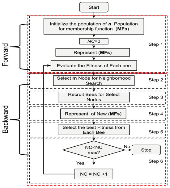
Figure 1.
Visual step-by-step representation of the BCO algorithm.
3.2. Proposed Fuzzy BCO Algorithm
A T1FLS was proposed by Lofti Zadeh in 1965 [51,52,53], and based on these ideas, Mendel et al. [54,55] formulated an IT2 FS , which is expressed as and Equations (5) and (6) describe each FS, and Figure 2 shows an IT2FLS [56,57].
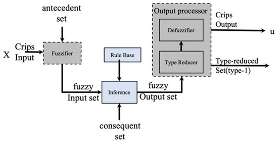
Figure 2.
Design of an IT2FLS.
The footprint of uncertainty (FOU) is the difference in the values of the upper MF (UMF) and the lower MF (LMF) in an IT2MF; the values of the UMF are always greater than or equal to the those of the LMF.
The IT2MF is created with the maximum UMF value always equal to 1 (normalized UMF). The LMF is created by reducing the UMF and then shifting both sides inward from the UMF. This scaling operation reduces the maximum LMF value, while the shifting operation introduces a lag in the LMF values relative to the UMF. Both the scaling and shifting operations define the FOU of a type-2 MF by interval. Both the scale (lowerScale) and lag values (lowerLag) vary between 0 and 1. The lag value is expressed as the UMF values, where the LMF values vary between zero and non-zero values. The lag values can be different on the left and right sides to produce asymmetric FOUs. Figure 3 represents an example of a trapezoidal MF.
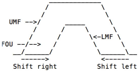
Figure 3.
Design of a trapezoidal MF in an IT2FLS.
The UMF parameters are a numeric vector that specifies the values of the UMF. The lowerScale parameter is a numeric scalar specification scale factor for the LMF. Similarly, the lowerLag parameter is a vector that specifies the lag values for the LMF. Figure 4 shows a representation of an IT2FM.
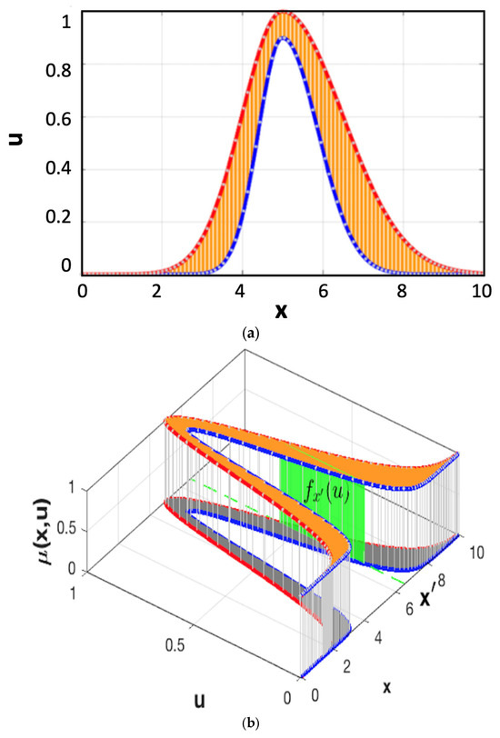
Figure 4.
Representation of a Gaussian type-2 MF in 2-D (a) and 3-D (b) space.
The proposed type of MF is a triangular MF: The TriScaleTriInterval2MF (x,{{[a, b, c]}, ,}) is denoted by , which is defined by the triangular FOU () with parameters for the UMF and the parameters are and for the LMF, which defines . Figure 5 shows the visual representation of the TriScaleTriIntervalT2MF and Equation (7) is the mathematical representation.
Or, the following Heaviside function (H) can be used to join the segments of each interval of the function (x):
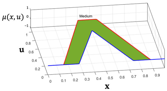
Figure 5.
Graphical illustration of the TriScaleTriIntervalT2MF.
The LMF support, (x), is defined by the values p and q, which are functions of the UMF parameters (a, b, c), (x), and the elements of ℓ. The design and construction of a triangular MF IT2FLS is represented by Equation (9). The mathematical expression is shown in Equation (9):
The function (x) is multiplied by the lowerScale (λ) to form the LMF, (x), which is described as or by using the Heaviside function (H) to join the segments of each interval of the function, μ(x), as shown in Equation (10):
The structure of the rules is the Takagi–Sugeno–Kang T2FLS structure, which is defined below. The fuzzy rules are detailed in Table 1. For a T2FL with n inputs and one output , if we suppose M rules, the kth rule in the IT2FLS can be expressed as Equation (11) [58,59], which is as follows:
where the coefficients are type-2 interval fuzzy numbers. The IT2 TSK FSs that employ these rules are called (A2-C1); this means that the antecedents are IT2FSs while the consequents are T2FSs. The coefficient is the center and is the ratio of uncertainty of interval . To simplify , the linear functions of the TSK rules are obtained. Equations (13) and (14) show this expression.
where

Table 1.
Fuzzy rules of the proposal SIT2FLS-FBCO.
A visualization of the proposed SIT2FLS-BCO is shown in Figure 6.
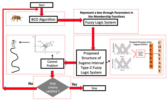
Figure 6.
Visualization of the proposed SIT2FLS-FBCO.
The main idea of the method was proposed in [48]; here, the goal was to utilize the Takagi–Sugeno method in an IT2FLS. Excellent results using this method for stabilization in control problems were demonstrated in [60,61,62,63]. In this proposal, the first variable is the iteration. The following Equation (15) shows the mathematical representation [48]:
Diversity is the second variable and is expressed by Equation (16), which measures the dispersion degree of the bees, an important metric in designing the fuzzy rules in the SIT2FLS-FBCO [48], and is as follows:
where the current iteration is t, the population size is , a bee is denoted by i, the total number of solutions is , and the next solution is given by j. For a bee i, its solution j is indicated by ; in the end, the solution j for the best bee is given by j [48]. The SIT2FLS is illustrated in Figure 7.
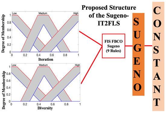
Figure 7.
Structure of the proposed SIT2FLS-FBCO.
The execution begins with a high exploration value () and low exploitation value (). Therefore, Iterations and Diversity have low values. Based on this reasoning, rule 5 states that “If Iterations and Diversity are Medium, then and are Medium”. The analysis was based on the following idea: when is a high value, this indicates a medium level of exploration (value of 0.5) and when is 0.5, it indicates a medium level of exploitation. When Iterations is high, the bees have high Diversity and the value of is low to achieve a low level of exploration and the value of is high to achieve better exploitation (rule 9). In the opposite rule, when Iterations is low, the bees have low Diversity and the value of is high to achieve a high level of exploration and the value is low to achieve a low level of exploitation (see fuzzy rule 1). Therefore, based on the design of the fuzzy rules, at the beginning of BCO, Iterations is low and Diversity is low, and the aim is to achieve greater exploration and exploitation using the algorithm: the design of each fuzzy rule is based on this reasoning. For example, rule number 3 states that “If Iterations is Low and Diversity is High, then Beta is MediumHigh and Alpha is MediumLow”. Based on this reasoning, rule number 7 states that “If Iterations is High and Diversity is Low, then Beta is Medium and Alpha is High”. According to the analysis of the results from applying this rule, when has a medium value, this indicates a medium level of exploration and when has a value of 0.9 or 1, this indicates a high level of exploitation.
In BCO, the value of the population (all virtual bees) is denoted by “NC”, the total number of constructive moves that one bee realizes is denoted by “ScoutBees”, and finally, each possible good solution that a bee finds during the execution is denoted by “FollowerBees”. This is shown visually in Figure 8. Table 1 shows the nine rules, and a representation of the surface of the SIT2FLS-FBCO is shown in Figure 9.
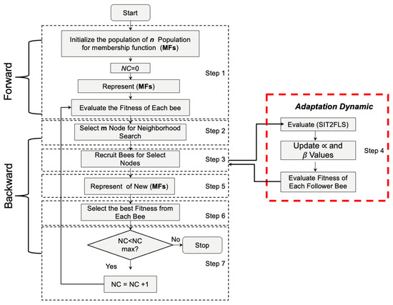
Figure 8.
Flowchart of the fuzzy BCO with SIT2FLS.
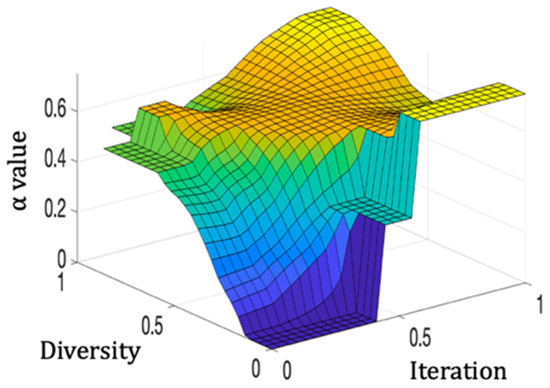
Figure 9.
Surface of the SIT2FLS.
4. Case Study
In this case study, the problem involves a unicycle mobile robot [22,23,64]. Computationally, an IT2FLS finds optimal solutions with fewer iterations based on the metaheuristic of the bee colony compared to a T1FLS when the scenarios are under perturbations. This allows the system to be used in real-world problems, such as trajectory optimization, by considering the perturbation levels expressed later hen finding the desired trajectory. The proposed method allows for better stabilization of the case study object when noise is added in the experiments. Figure 10 illustrates the case study. The mathematical representation is given in Equations (17) and (18).
where is the configuration coordinates vector, is the velocity vector, is the vector representing the wheels ( = right and = left), is a uniformly bounded disturbance vector, is the positive definite inertia matrix, is the vector of the Coriolis and centripetal forces, and is from Equation (15).
where are the reference positions. The -axis indicates the (linear velocity) and (angular velocity) in the . Equation (16) represents a non-slip wheel condition.
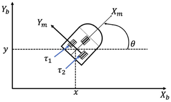
Figure 10.
Robot representation.
The structure of the Mamdani T1FLS is shown in Figure 11. The rules are described in Table 2 and Figure 12 shows the model [48]. Table 3 shows the results of the rules.
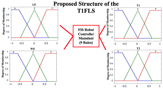
Figure 11.
Design of the T1FLS.
Table 2.
Fuzzy rules of the Mamdani T1FLS.
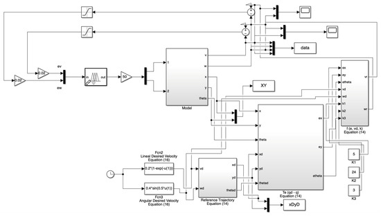
Figure 12.
Fuzzy logic controller for an AMR.
Table 3.
Results from original BCO, MFBCO-IT2FLS, and SIT2FLS (normal and reverse trajectories) without disturbance.
5. Experimental Results
The testing consisted of 30 experiments. The BCO used a total of 50 populations (virtual bees), with 25 following bees. A total of 30 iterations were executed and the values of the and parameters were found dynamically. Two types of trajectories were considered in the experiments (see Figure 13), and three types of perturbations in the model were tested (see Table 4). The objective function that was used was the mean square error (MSE) function, which is shown in Equation (17). Table 1 shows the results from the original BCO, MIT2FLS-FBCO, and SIT2FLS-FBCO with the two types of trajectories (normal and reverse); the results from FBCO using an interval type-3 FLS are also shown in Table 3.
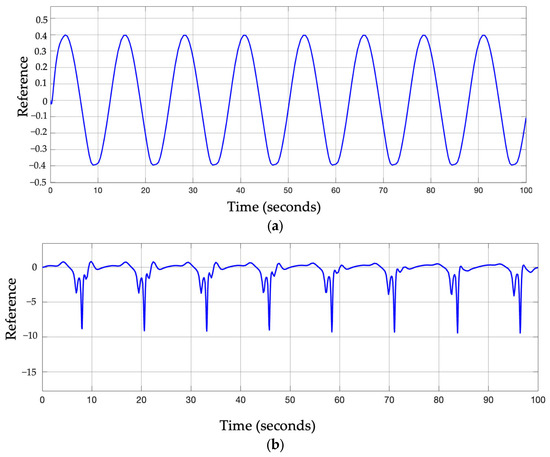
Figure 13.
Visual representation with the two types of trajectories in the simulations. (a) Normal trajectory; (b) reverse trajectory.
Table 4.
Disturbances applied to the controller.
In Table 3, the best average MSE value (3.13 × 10⁻¹) was obtained with the proposed SIT2FLS-FBCO and the normal trajectory was used compared to the MIT2FLS-FBCO with an MSE value of 3.23 × 10⁻¹ and the original BCO with fixed values of and an MSE value of 3.75 × 10⁻¹. The best minimal error (best MSE) was obtained with the proposed Sugeno IT2FLS-FBCO (1.03 × 10⁻³ compared to 1.19 with the Mamdani IT3FLS-FBCO).
To analyze the performance of the proposed system, three types of disturbances were tested. The types of errors were selected to evaluate the performance of the proposed system. Each type of error represents an obstacle that the robot may encounter in the real world when following a desired route. These errors are different types of disturbances that the SIT2FLS-FBCO must adapt to. The values assigned to each type of disturbance were selected by trial and error based on previous works [22,23,25]. Table 4 summarizes the details of the settings for each perturbation. Two types of trajectories were used to observe the performance of the proposed SIT2FLS-FBCO; Figure 13 illustrates each trajectory. Table 5 lists the experimental results with the normal trajectory.
Table 5.
Experimental results with the different types of disturbances with the SIT2FLS-FBCO with a normal trajectory.
Table 6.
Experimental results with the different types of disturbances with the Sugeno FBCO-IT2FLS with a reverse trajectory.
In Table 5 and Table 6, the best average MSE results were obtained with the proposed SIT2FLS-FBCO and band-limited white noise as the type of disturbance with both normal and reverse trajectories. This is because the disturbance did not affect the stability when the SIT2FLS-FBCO was implemented in the FLC, and the stabilization of the AMR was better when compared to the other types of disturbances. Another important observation was that the reverse trajectory yielded better results (average MSE) than the proposed method. This is because it was better at analyzing the uncertainty. Thus, using the reverse trajectory makes the proposed method better at analyzing the exploration using the FBCO algorithm compared to using the normal trajectory.
6. Discussion
6.1. Comparison of the Results with the Original BCO, MIT2FLS-FBCO, and SIT2FLS-FBCO
Table 1 shows that there were smaller errors with the proposed SIT2FLS-FBCO compared with the MIT2FLS-FBCO and original BCO. Figure 14 illustrates the changes in the MSE with each method.
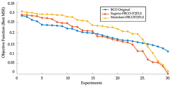
Figure 14.
Comparison of results with original BCO, SIT2FLS-FBCO, and MIT2FLS-FBCO.
Figure 14 shows that the SIT2FLS-FBCO (orange line) produced better stabilization compared to the original BCO and MIT2FLS-FBCO.
A comparison of the best results with the different types of perturbation implemented in normal and reverse trajectories is illustrated in Figure 15 along with the LE output. The red line is used to represent the desired trajectory and the blue line is used to represent the trajectory found with the proposal.
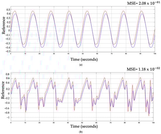
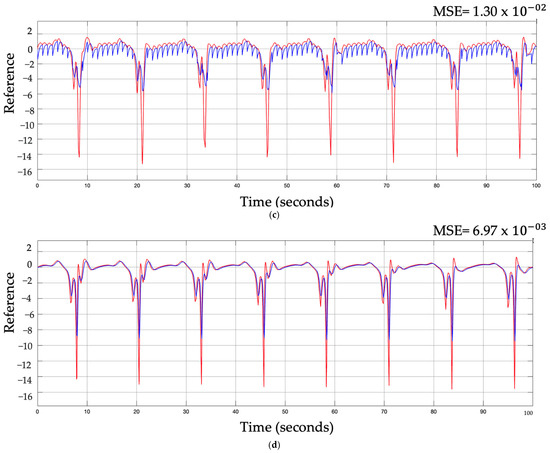
Figure 15.
Comparison of results with different trajectories and disturbances. (a) Best results for original BCO without disturbance and normal trajectory; (b) best results for SIT2FLS-BCO with band-limited white noise disturbance and normal trajectory; (c) best results for original BCO without disturbance and with reverse trajectory; (d) best results for SIT2FLS-BCO with band-limited white noise disturbance and reverse trajectory.
Visual comparisons of the behavior of the SIT2FLS-BCO without disturbance and with the three types of perturbation in the normal and reverse trajectories are shown in Figure 16 and Figure 17.
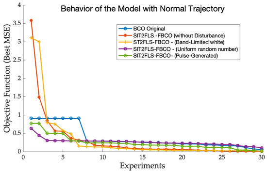
Figure 16.
Convergence of the proposed FBCO-SIT2FLS with different types of disturbances in the normal trajectory.
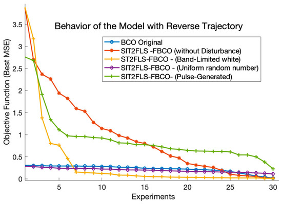
Figure 17.
Convergence of the proposed FBCO-SIT2FLS with different types of disturbances in the reverse trajectory.
Figure 16 shows a stabilization in the normal trajectory when the disturbance to the controller was band-limited white noise (yellow line). Figure 17 shows the results obtained with the reverse trajectory compared to the original BCO and with different types of disturbances.
Figure 17 shows a stabilization in the reverse trajectory when there was a disturbance to the controller, especially band-limited white noise (yellow line). For this type of trajectory, the best results were obtained when the type of disturbance was uniform random number or band-limited white noise.
6.2. Statistical Tests
Statistical tests of the results with the original BCO, Mamdani FBCO, and Sugeno FBCO and the different types of disturbances to the controller were performed. Table 7 shows the settings for the statistical tests.
Table 7.
Settings of parameters for statistical tests.
The hypotheses were as follows. Ho: The results of the SFBCO-IT2FLS are better or similar to those of the original BCO with random values. Ha: The results of the SFBCO-IT2FLS are worse than those of the original BCO. The results for a sample of 30 randomly chosen values are shown in Table 1, Table 3 and Table 4. The z-test is expressed by Equation (21), which is as follows:
If the Z value is smaller than −1.645, then the evidence is “Significant” (S) and the null hypothesis is rejected while the alternative hypothesis is accepted (the SFBCO-IT2FLS is better than BCO). The best results were obtained with band-limited white noise; therefore, the results from this type of disturbance were analyzed using the statistical tests. Table 8 shows the results with the different types of disturbances to the controller.
Table 8.
Results of the test comparing the SIT2FLS-FBCO to BCO.
The results in Table 8 show that the proposed SIT2LFS-FBCO with the band-limited white noise disturbance had significant evidence to reject the null hypothesis. The only test that was not significant (NS) was when the reverse trajectory was used (see test number 5) and when the proposed SIT2FLS-BCO was compared with the original BCO and MIT2FLS-FBCO.
Based on the analysis of the computational complexity of the fuzzy models, the reduction algorithms for T2FLSs and IT1FLSs based on the Sugeno–Takagi theory are very efficient in calculating the outputs, assuming that the primary variable x is sampled into N points and the secondary variable u(x) into M points. Therefore, a T1FLS has a computational complexity of O(N) [56,57] and the computational complexity of an IT2FLS is O(KN), where K represents the number of iterations needed to reach a switch point [59,62,64].
7. Conclusions
In conclusion, we found better stabilization of the controller using the SIT2FLS-FBCO because we were able to find the best values for and In the real world, controlling the stabilization of a robot’s trajectory is a complicated task because of challenges, such as obstacles or trajectory changes, that may arise. This is why this work included two types of trajectories, as well as the implementation of different types of disturbances that were applied to the FLC. In conclusion, compared to the MIT2LFS-FBCO and original BCO with values of = 0.5 and = 2.5, the SIT2FLS-FBCO produced better results.
The results showed that the SIT2LFS-FBCO was superior to the original BCO (Figure 14). Figure 16 and Figure 17 illustrate the excellent stabilization, reflected by the lower errors, with the SIT2LFS-FBCO when different types of disturbances to the FLC were simulated.
The recommended values for the and parameters, according to the proposed method, can be found using the average of the results from the disturbance models. The best results were obtained with the SFBCO-IT2FLS with band-limited white noise as the disturbance; we recommend values of 0.474 for and 2.40 for .
In future work, the Takagi–Sugeno FBCO-IT2FLS will be applied to real-world problems, such as controlling the stabilization of a drone, the stabilization in cruise control, or the stabilization of an inverted pendulum. Another important direction could be to optimize fuzzy controllers with greater uncertainty values, for example, an IT2FLC using the Takagi–Sugeno inference method, or to optimize the parameters for a generalized IT2FLS or an interval type-3 FLS using FBCO.
Author Contributions
Conceptualization, writing—review and editing and formal analysis, L.A.-A.; supervision, funding, methodology and validation, P.M.; methodology and validation, O.C. All authors have read and agreed to the published version of the manuscript.
Funding
This research received funding from TecNM under the hybrid intelligent systems academic group ITTIJ-CA-1.
Data Availability Statement
Data are contained within the article.
Acknowledgments
We thank the Division of Graduate Studies and Research of Tijuana Institute of Technology for the support for our research and for creating an excellent team that collaborated with all the authors on this paper.
Conflicts of Interest
The authors declare no conflicts of interest.
Abbreviations
The following abbreviations are used in this manuscript:
| IT2FLS | Interval type-2 fuzzy logic system |
| BCO | Bee Colony Optimization |
| FBCO | Fuzzy Bee Colony Optimization |
| AMR | Autonomous Mobile Robot |
| FLC | Fuzzy Logic Controller |
| T1FLS | Type-1 fuzzy logic system |
| MIT2FLS | Mamdani interval type-2 fuzzy logic system |
| UMF | Upper Membership Function |
| MFs | Membership functions |
| LMF | Lower Membership Function |
| LE | Linear Error |
| WE | Angular Error |
| FOU | Footprint of uncertainty |
| FS | Fuzzy Set |
| FLS | Fuzzy logic system |
| PID | Proportional Integral Differential |
| FIS | Fuzzy inference system |
| IT2MFs | Interval type-2 membership functions |
References
- Alizadeh, M.H.; Toloei, A. Designing Pitch Angle Compensator for an UAV and Robustification it with Bee Colony Optimization Algorithm. Technol. Aerosp. Eng. 2024, 8, 1–14. [Google Scholar]
- Holliday, A.; Dudek, G. Neural Bee Colony Optimization: A Case Study in Public Transit Network Design. arXiv 2023, arXiv:2306.00720. [Google Scholar]
- Ramezanzadeh, F.; Shokrzadeh, H. Efficient routing method for IoT networks using bee colony and hierarchical chain clustering algorithm. Electr. Eng. Electron. Energy 2024, 7, 100424. [Google Scholar] [CrossRef]
- Ramzan, M.S.; Asghar, A.; Ullah, A.; Alsolami, F.; Ahmad, I. A Bee Colony-Based Optimized Searching Mechanism in the Internet of Things. Future Internet 2024, 16, 35. [Google Scholar] [CrossRef]
- Liang, W.; Qian, B.; Hu, R.; Zhang, Z.; Zhang, C. Two stage bee colony algorithm for hot rolling scheduling problem in compact strip production. Comput. Integr. Manuf. Syst. 2025, 31, 102. [Google Scholar]
- Shi, J.; Tong, B.; Liu, J.; Chen, Z.; Li, P.; Tan, C. Feature Variable Selection for Near-Infrared Spectroscopy Based on Simulated Annealing Bee Colony Algorithm. J. Chemom. 2025, 39, e3633. [Google Scholar] [CrossRef]
- Khamsen, W.; Takeang, C.; Janthawang, T.; Aurasopon, A. A novel multi-objective economic load dispatch solution using bee colony optimization method. Int. J. Electr. Comput. Eng. 2025, 15, 1385–1395. [Google Scholar] [CrossRef]
- Gupta, M.; Pandey, S.K.; Pareek, P.K.; Shukla, P.K.; Aggarwal, P.K.; Reddy, P.V. Efficient Routing and Lifetime Prolongation in IoT founded Wireless Sensor Network Performance with Bee Colony-Inspired Lifetime Enhancement. J. Intell. Syst. Internet Things 2025, 14, 221–229. [Google Scholar]
- Abid, M.; Yadav, A.S. Modeling and Optimizing blood supply chain inventory management using bee colony and genetic algorithms. Cuest. De Fisioter. 2025, 54, 2068–2095. [Google Scholar]
- Nikolić, M.; Rakas, J.; Teodorović, D. Solving the aircraft landing problem using the bee colony optimization (BCO) algorithm. Adv. Comput. 2024, 135, 51–76. [Google Scholar]
- Modey, P.; Abdul-Salaam, G.; Freeman, E.; Acheampong, P.; Brown-Acquaye, W.L.; Agbehadji, I.E.; Millham, R.C. K-Means Based Bee Colony Optimization for Clustering in Heterogeneous Sensor Network. Sensors 2024, 24, 7603. [Google Scholar] [CrossRef] [PubMed]
- Xiao, L.; Wang, X.; Chen, F.; Li, A. Fuzzy proportional integral differential control of magnetorheological clutch torque based on bee colony algorithm optimization. J. Vib. Control 2024, 30, 5450–5460. [Google Scholar] [CrossRef]
- Dasarathy, A.K.; Saxena, S.; Soni, M.; Sasi, M. Machine Learning-Based Movement Scheduling and Management for Autonomous Mobile Robot Navigation. Int. J. Intell. Syst. Appl. Eng. 2024, 12, 398–405. [Google Scholar]
- Preetha, M.; Archana, A.B.; Ragavan, K.; Kalaichelvi, T.; Venkatesan, M. A Preliminary Analysis by using FCGA for Developing Low Power Neural Network Controller Autonomous Mobile Robot Navigation. Int. J. Intell. Syst. Appl. Eng. 2024, 12, 39–42. [Google Scholar]
- Vignesh, C.; Uma, M.; Sethuramalingam, P. Development of rapidly exploring random tree based autonomous mobile robot navigation and velocity predictions using K-nearest neighbors with fuzzy logic analysis. Int. J. Interact. Des. Manuf. (IJIDeM) 2024, 18, 4547–4571. [Google Scholar] [CrossRef]
- Pakkala, D.; Känsäkoski, N.; Heikkilä, T.; Backman, J.; Pääkkönen, P. On design of cognitive situation-adaptive autonomous mobile robotic applications. Comput. Ind. 2025, 167, 104263. [Google Scholar] [CrossRef]
- Tang, Y.; Zakaria, M.A.; Younas, M. Path Planning Trends for Autonomous Mobile Robot Navigation: A Review. Sensors 2025, 25, 1206. [Google Scholar] [CrossRef] [PubMed]
- Ušinskis, V.; Nowicki, M.; Dzedzickis, A.; Bučinskas, V. Sensor-Fusion Based Navigation for Autonomous Mobile Robot. Sensors 2025, 25, 1248. [Google Scholar] [CrossRef]
- Bhuvaneswari, M.; Elango, C.; Jagadeeshwaran, S.; Riyaz, J.S. Design and fabrication of robotic operating system based autonomous mobile robot for education and material handling purpose. AIP Conf. Proc. 2025, 3204, 030019. [Google Scholar]
- Göktaş, A.G.; Sezer, S. A New Local Path Planning Approach by Synthesis of PRM and RRT* Algorithms for an Autonomous Mobile Robot. J. Control Autom. Electr. Syst. 2025, 36, 72–85. [Google Scholar] [CrossRef]
- Bai, H.; Yang, P.; Qin, Z.; Qi, M.; Xiong, W. Order sequencing, tote scheduling, and robot routing optimization in multi-tote storage and retrieval autonomous mobile robot systems. Int. J. Prod. Res. 2025, 63, 314–341. [Google Scholar] [CrossRef]
- Amador-Angulo, L.; Castillo, O.; Melin, P.; Castro, J.R. Interval type-3 fuzzy adaptation of the bee colony optimization algorithm for optimal fuzzy control of an autonomous mobile robot. Micromachines 2022, 13, 1490. [Google Scholar] [CrossRef]
- Amador-Angulo, L.; Castillo, O. Optimization of Fuzzy Trajectory Tracking in Autonomous Mobile Robots Based on Bio-inspired Algorithms. In Recent Advances of Hybrid Intelligent Systems Based on Soft Computing; Springer: Cham, Switzerland, 2020; pp. 249–271. [Google Scholar]
- Zou, A.; Wang, L.; Li, W.; Cai, J.; Wang, H.; Tan, T. Mobile robot path planning using improved mayfly optimization algorithm and dynamic window approach. J. Supercomput. 2023, 79, 8340–8367. [Google Scholar] [CrossRef]
- Amador-Angulo, L.; Castillo, O.; Melin, P.; Geem, Z.W. Type-3 fuzzy dynamic adaptation of Bee colony optimization applied to mathematical functions. Fuzzy Sets Syst. 2024, 489, 109014. [Google Scholar] [CrossRef]
- Priyaradhikadevi, T.; Vijayakumari, P.; Balaji, M.; Chinnammal, V.; Vijay, S. Revolutioning WSN: Experimental Design of an Energy Efficient Communication Protocol Using Improved BEE Colony Clustering Model. In Proceedings of the 2024 International Conference on Advances in Computing, Communication and Applied Informatics (ACCAI), Chennai, India, 9–10 May 2024; IEEE: Piscataway, NJ, USA, 2024; pp. 1–7. [Google Scholar]
- Yu, Q.; Qi, X.; Zhang, Y.; Duan, H. Multi-Objective Optimization of Reactive Power for Grid-Connected Photovoltaic Power Plants Based on Improved Bee Colony Algorithm. In Proceedings of the 2024 IEEE 7th International Electrical and Energy Conference (CIEEC), Harbin. China, 10–12 May 2024; IEEE: Piscataway, NJ, USA, 2024; pp. 2323–2329. [Google Scholar]
- Liu, B.; Zhou, W.; Ren, H.; Fan, Z. Intelligent Prediction and Data Service Optimization Scheme of Power Grid Based on Improved Bee Colony Algorithm. J. Inf. Hiding Multimed. Signal Process. 2024, 9, 253–272. [Google Scholar]
- Palominos, P.; Mazo, M.; Fuertes, G.; Alfaro, M. An Improved Marriage in Honey-Bee Optimization Algorithm for Minimizing Earliness/Tardiness Penalties in Single-Machine Scheduling with a Restrictive Common Due Date. Mathematics 2025, 13, 418. [Google Scholar] [CrossRef]
- Castillo, O.; Melin, P.; Ontiveros, E.; Peraza, C.; Ochoa, P.; Valdez, F.; Soria, J. A high-speed interval type 2 fuzzy system approach for dynamic parameter adaptation in metaheuristics. Eng. Appl. Artif. Intell. 2019, 85, 666–680. [Google Scholar] [CrossRef]
- Guerrero, M.; Valdez, F.; Castillo, O. Comparative study between type-1 and interval type-2 fuzzy systems in parameter adaptation for the cuckoo search algorithm. Symmetry 2022, 14, 2289. [Google Scholar] [CrossRef]
- Shirgir, S.; Farahmand-Tabar, S. An enhanced optimum design of a Takagi-Sugeno-Kang fuzzy inference system for seismic response prediction of bridges. Expert Syst. Appl. 2025, 266, 126096. [Google Scholar] [CrossRef]
- Sain, D.; Praharaj, M.; Mohan, B.M.; Yang, J.M. Takagi–Sugeno fractional-order interval type-2 fuzzy proportional–integral–derivative controller with real-time application to a magnetic levitation system. Comput. Electr. Eng. 2025, 123, 110001. [Google Scholar] [CrossRef]
- Dong, B.T.; Nguyen, T.V.A. Reconstructing Membership Functions for Observer-Based Controller Design of Takagi–Sugeno Fuzzy Model with Unmeasured Premise Variables. Int. J. Fuzzy Syst. 2025, 1–14. [Google Scholar] [CrossRef]
- Ringwood, J.V.; Farajvand, M.; García-Violini, D. Takagi-Sugeno fuzzy modelling for wave energy converters. In Innovations in Renewable Energies Offshore; CRC Press: Boca Raton, FL, USA, 2025; pp. 543–550. [Google Scholar]
- Ozcan, O.F.; Kilic, H.; Ozguven, O.F. A unified robust hybrid optimized Takagi–Sugeno fuzzy control for hydrogen fuel cell-integrated microgrids. Int. J. Hydrog. Energy, 2025; in press. [Google Scholar] [CrossRef]
- Pourasghar, M.; Nguyen, A.T.; Guerra, T.M. Guaranteed State Estimation for Fault Detection of Uncertain Takagi-Sugeno Fuzzy Systems With Unmeasured Nonlinear Consequents. IEEE Trans. Fuzzy Syst. 2025, 1–12. [Google Scholar] [CrossRef]
- Nguyen, V.T.; Pham, D.H.; Nguyen-Xuan, H.; Nguyen, Q.C. Optimal Design of Takagi-Sugeno-Kang Fuzzy Neural Network Based on Balancing Composite Motion Optimization for Chaotic Synchronization with Uncertainty and Disturbance. Results Eng. 2025, 25, 104234. [Google Scholar] [CrossRef]
- Herizi, A.; Bouguerra, A.; Zeghlache, S.; Rouabhi, R.; Smaini, H.E.; Mahmoudi, R. Type-2 Sugeno fuzzy logic inference system for speed control of a doubly-fed induction motor. In Proceedings of the 1st International Conference on Digitization and Its Applications, Sharjah, United Arab Emirates, 2–4 December 2019. [Google Scholar]
- Chen, Y.; Xi, J.; Wang, H.; Liu, X. Grey wolf optimization algorithm based on dynamically adjusting inertial weight and levy flight strategy. Evol. Intell. 2023, 16, 917–927. [Google Scholar] [CrossRef]
- Vijaya, C.; Srinivasan, P. Hybrid Fuzzy Metaheuristic Technique for Efficient VM Selection and Migration in Cloud Data Centers. Informatica 2024, 48, 20. [Google Scholar] [CrossRef]
- Amador-Angulo, L.; Castillo, O. An interval type-2 fuzzy logic approach for dynamic parameter adaptation in a whale optimization algorithm applied to mathematical functions. Axioms 2023, 13, 33. [Google Scholar] [CrossRef]
- Teodorović, D. Bee colony optimization (BCO). In Innovations in Swarm Intelligence; Springer: Berlin/Heidelberg, Germany, 2009; pp. 39–60. [Google Scholar]
- Teodorović, D.; Davidović, T.; Šelmić, M.; Nikolić, M. Bee Colony Optimization and its Applications. In Handbook of AI-Based Metaheuristics; CRC Press: Boca Raton, FL, USA, 2021; pp. 301–322. [Google Scholar]
- Teodorovic, D.; Davidovic, T.; Selmic, M. Bee colony optimization Part II: The applications survey. Yugosl. J. Oper. Res. 2015, 25, 185–219. [Google Scholar] [CrossRef]
- Davidovic, T.; Teodorovic, D.; Selmic, M. Bee colony optimization Part I: The algorithm overview. Yugosl. J. Oper. Res. 2016, 25, 33–56. [Google Scholar] [CrossRef]
- Krüger, T.J.; Davidović, T.; Teodorović, D.; Šelmić, M. The bee colony optimization algorithm and its convergence. Int. J. Bio-Inspired Comput. 2016, 8, 340–354. [Google Scholar] [CrossRef]
- Amador-Angulo, L.; Mendoza, O.; Castro, J.R.; Rodríguez-Díaz, A.; Melin, P.; Castillo, O. Fuzzy sets in dynamic adaptation of parameters of a bee colony optimization for controlling the trajectory of an autonomous mobile robot. Sensors 2016, 16, 1458. [Google Scholar] [CrossRef]
- Biesmeijer, J.C.; Seeley, T.D. The use of waggle dance information by honey bees throughout their foraging careers. Behav. Ecol. Sociobiol. 2005, 59, 133–142. [Google Scholar] [CrossRef]
- Dyler, F.C. The biology of the dance language. Annu. Rev. Entomol. 2002, 47, 917–949. [Google Scholar]
- Zadeh, L.A. Fuzzy sets. Inf. Control 1965, 8, 338–353. [Google Scholar] [CrossRef]
- Zadeh, L.A. Fuzzy logic. In Granular, Fuzzy, and Soft Computing; Springer: New York, NY, USA, 2023; pp. 19–49. [Google Scholar]
- Zadeh, L.A. The concept of a Linguistic Variable and its Application to Approximate Reasoning, Part II. Inf. Sci. 1975, 8, 301–357. [Google Scholar] [CrossRef]
- Mendel, J.M.; John, R.B. Type-2 fuzzy sets made simple. IEEE Trans. Fuzzy Syst. 2002, 10, 117–127. [Google Scholar] [CrossRef]
- Mendel, J.M. Uncertain rule-based fuzzy systems. In Introduction and New Directions; Springer: Cham, Switzerland, 2017; 580p. [Google Scholar]
- Mendel, J.M.; John, R.I.; Liu, F. Interval type-2 fuzzy logic systems made simple. IEEE Trans. Fuzzy Syst. 2006, 14, 808–821. [Google Scholar] [CrossRef]
- Karnik, N.N.; Mendel, J.; Liang, Q. Type-2 fuzzy logic systems. IEEE Trans. Fuzzy Syst. 1999, 7, 643–658. [Google Scholar] [CrossRef]
- Liang, Q.; Mendel, J.M. Interval type-2 fuzzy logic systems: Theory and design. IEEE Trans. Fuzzy Syst. 2000, 8, 535–550. [Google Scholar] [CrossRef]
- Karnik, N.N.; Mendel, J.M. Introduction to type-2 fuzzy logic systems. In Proceedings of the 1998 IEEE International Conference on Fuzzy Systems Proceedings. IEEE World Congress on Computational Intelligence (Cat. No. 98CH36228), Anchorage, AK, USA, 4–9 May 1998; IEEE: Piscataway, NJ, USA, 1998; Volume 2, pp. 915–920. [Google Scholar]
- Mehran, K. Takagi-sugeno fuzzy modeling for process control. In Industrial Automation, Robotics and Artificial Intelligence (EEE8005); Newcastle University: Newcastle upon Tyne, UK, 2008; Volume 262, pp. 1–31. [Google Scholar]
- Chang, C.W.; Tao, C.W. A novel approach to implement Takagi-Sugeno fuzzy models. IEEE Trans. Cybern. 2017, 47, 2353–2361. [Google Scholar] [CrossRef]
- Benzaouia, A.; Hajjaji, A.E. Advanced Takagi-Sugeno Fuzzy Systems. In Studies in Systems, Decision and Control Book 8; Springer: Berlin/Heidelberg, Germany, 2014. [Google Scholar]
- Anikin, I.V.; Zinoviev, I.P. Fuzzy control based on new type of Takagi-Sugeno fuzzy inference system. In Proceedings of the 2015 International Siberian Conference on Control and Communications (SIBCON), Omsk, Russia, 20–23 May 2015; IEEE: Piscataway, NJ, USA, 2015; pp. 1–4. [Google Scholar]
- Castillo, O.; Amador-Angulo, L.; Castro, J.R.; Garcia-Valdez, M. A comparative study of type-1 fuzzy logic systems, interval type-2 fuzzy logic systems and generalized type-2 fuzzy logic systems in control problems. Inf. Sci. 2016, 354, 257–274. [Google Scholar] [CrossRef]
Disclaimer/Publisher’s Note: The statements, opinions and data contained in all publications are solely those of the individual author(s) and contributor(s) and not of MDPI and/or the editor(s). MDPI and/or the editor(s) disclaim responsibility for any injury to people or property resulting from any ideas, methods, instructions or products referred to in the content. |
© 2025 by the authors. Licensee MDPI, Basel, Switzerland. This article is an open access article distributed under the terms and conditions of the Creative Commons Attribution (CC BY) license (https://creativecommons.org/licenses/by/4.0/).