Article

Solving Fractional Stochastic Differential Equations via a Bilinear Time-Series Framework

by
Rami Alkhateeb
1,†,
Ma’mon Abu Hammad
2,†,
Basma AL-Shutnawi
3,*,
Nabil Laiche
4,5 and
Zouaoui Chikr El Mezouar
6
1
Department of Allied Sciences, AL-Ahliyya Amman University, Amman 19328, Jordan
2
Department of Mathematics, AL-Zaytoonah University of Jordan, Queen Alia Airport St. 594, Amman 11942, Jordan
3
Department of Mathematics, Tafila Technical University, P.O. Box 179, Tafila 66110, Jordan
4
Applied Mathematics Department, University of Seville, 41012 Seville, Spain
5
Dynamical Systems and Control Laboratory, Oum El Bouaghi University, Oum El Bouaghi 04000, Algeria
6
Department of Mathematics, College of Science, King Khalid University, Abha 62223, Saudi Arabia
*
Author to whom correspondence should be addressed.
These authors contributed equally to this work.
Symmetry 2025, 17(5), 764; https://doi.org/10.3390/sym17050764
Submission received: 20 March 2025 / Revised: 29 April 2025 / Accepted: 8 May 2025 / Published: 15 May 2025

Abstract

:
This paper introduces a novel numerical approach for solving fractional stochastic differential equations (FSDEs) using bilinear time-series models, driven by the Caputo–Katugampola (C-K) fractional derivative. The C-K operator generalizes classical fractional derivatives by incorporating an additional parameter, enabling the enhanced modeling of memory effects and hereditary properties in stochastic systems. The primary contribution of this work is the development of an efficient numerical framework that combines bilinear time-series discretization with the C-K derivative to approximate solutions for FSDEs, which are otherwise analytically intractable due to their nonlinear and memory-dependent nature. We rigorously analyze the impact of fractional-order dynamics on system behavior. The bilinear time-series framework provides a computationally efficient alternative to traditional methods, leveraging multiplicative interactions between past observations and stochastic innovations to model complex dependencies. A key advantage of our approach is its flexibility in handling both stochasticity and fractional-order effects, making it suitable for applications in a famous nuclear physics model. To validate the method, we conduct a comparative analysis between exact solutions and numerical approximations, evaluating convergence properties under varying fractional orders and discretization steps. Our results demonstrate robust convergence, with simulations highlighting the superior accuracy of the C-K operator over classical fractional derivatives in preserving system dynamics. Additionally, we provide theoretical insights into the stability and error bounds of the discretization scheme. Using the changes in the number of simulations and the operator parameters of Caputo–Katugampola, we can extract some properties of the stochastic fractional differential model, and also note the influence of Brownian motion and its formulation on the model, the main idea posed in our contribution based on constructing the fractional solution of a proposed fractional model using known bilinear time series illustrated by application in nuclear physics models.

1. Introduction

Nonlinear time-series analysis plays a pivotal role in various scientific disciplines, including economics [1], climate science, finance, and dynamic systems engineering. Throughout the 20th century, nonlinear time-series models have increasingly gained prominence over linear models due to their enhanced ability to capture complex and dynamic phenomena. Many real-world time series exhibit features such as asymmetry, regime shifts, and nonlinear dependence structures, which linear models are often inadequate to represent. Among the various nonlinear approaches, bilinear time-series models have emerged as particularly successful tools for modeling such intricacies in observed data. [2]. With rapid advances in economics and finance, there has been a significant proliferation of various types of nonlinear models [3]. This growth has necessitated the development of robust application tools capable of addressing the diverse characteristics of nonlinear time series. In this context, stochastic calculus has emerged as a critical tool, providing a powerful framework for modeling and analyzing complex financial data. A key aspect of this interplay is the fundamental relationship between stochastic processes and time-series analysis, rooted in the fact that the derivative of Brownian motion corresponds to white noise [4]. This connection establishes a direct link between continuous-time stochastic models and discrete-time data [5,6,7] reinforcing the role of stochastic differential equations in capturing intricate economic and financial phenomena; see [8,9]. As a result, stochastic calculus has emerged as a powerful framework for modeling financial markets, macroeconomic trends, and risk assessment [10,11,12], bridging theoretical advancements with real-world forecasting and decision making [13].
Among the tools increasingly used in modeling and estimation are fractional differential equations; see [14,15,16,17]. This emerging field has attracted a large community of scientists, not only mathematicians but also statisticians, physicists, engineers, and researchers in medicine and microbiology, among others. Fractional derivatives have emerged as a powerful mathematical tool for modeling complex systems that exhibit memory effects, non-local behaviors, and anomalous dynamics. Unlike classical integer-order derivatives, fractional derivatives capture the history and long-range dependencies of a system [18], making them particularly suitable for describing phenomena in physics [19], biology, economics, and engineering. Their ability to model systems with memory and hereditary properties has revolutionized the way we understand and analyze dynamic processes, especially those that cannot be adequately described by traditional differential equations. In the context of nonlinear time-series analysis, fractional derivatives play a crucial role in capturing the intricate dynamics of real-world data [20]. Nonlinear time series are ubiquitous in scientific and engineering applications, ranging from financial markets and climate systems to biological processes and mechanical vibrations [21]. These systems often exhibit asymmetric behaviors, regime shifts, and nonlinear dependence structures that linear models fail to represent accurately.
Fractional derivatives play a crucial role in modeling nonlinear time series, particularly in finance and economics. Traditional models like ARIMA and GARCH fail to capture long memory effects and stochastic volatility in financial data. Fractional stochastic differential equations (FSDEs), incorporating fractional derivatives, provide a more robust framework, with applications such as fractional Brownian motion for financial time series. Beyond finance, fractional derivatives are used in climate science for modeling long-term temperature and precipitation patterns and in engineering for analyzing viscoelastic materials and memory-dependent control systems. Their flexibility enables deeper insights into complex system dynamics across various fields. Then, fractional stochastic differential equations (FSDEs) were developed to model systems with memory effects and randomness. Combining fractional calculus, which captures long-range dependencies, with stochastic processes, FSDEs provide a robust framework for analyzing complex dynamics in finance, physics, and biology. This type of equation is difficult to solve exactly because it combines the fractional derivative operator and Brownian motion.
Numerous researchers and computational scientists have focused on the numerical resolution of fractional stochastic differential equations ( FSDEs), as obtaining exact solutions often involves stringent constraints. To address these challenges, modern approaches have been developed, such as the numerical approximation of the Caputo–Katugampola operator [22,23,24,25,26,27] and the finite-differences method. Furthermore, discretization techniques using nonlinear time series have emerged as a powerful tool to solve FSDEs [28].
The choice of the Caputo–Katugampola (CK) fractional operator in this study is motivated by its versatility and enhanced modeling capabilities compared to classical fractional derivatives. Unlike the standard Caputo or Riemann–Liouville operators, the CK derivative incorporates an additional parameter, which provides greater flexibility in adjusting the kernel structure and memory effects of fractional differential equations. Its mathematical tractability also facilitates efficient numerical discretization, which is crucial for approximating solutions using bilinear time-series models. By leveraging the CK operator, our approach achieves a more accurate and adaptable framework for solving stochastic fractional differential equations, combining the strengths of fractional calculus with modern computational techniques. This makes the method particularly valuable for applications requiring high precision in capturing long-range dependencies and nonlinear stochastic behaviors. for more detailes redear can refer to [29,30,31,32].
This study presents a novel numerical approximation for solving stochastic fractional differential equations (SFDEs) using bilinear time-series models, combined with the Caputo–Katugampola fractional operator. Unlike traditional approaches, our method leverages the flexibility of bilinear models to capture nonlinear dynamics while incorporating the generalized fractional framework of the Caputo–Katugampola derivative. This enables efficient and accurate simulations of complex stochastic systems with memory effects. The proposed technique advances computational methods for SFDEs by bridging time-series analysis with modern fractional calculus, offering improved applicability in physics, finance, and engineering. Numerical results demonstrate the effectiveness of this approach in handling both stochasticity and fractional-order dynamics. The paper is structured as follows. Section 2 provides the foundational principles of stochastic calculus and their connection to bilinear time-series models, backgrounds to fractional differential calculus, and a theoretical review of three key concepts: bilinear time-series models, Section 3 establishes the theoretical framework and methodologies for a class of stochastic differential equations, extending their analysis through discretization using the Caputo–Katugampola operator. Section 4 focuses on constructing numerical solutions for these equations. Finally, Section 5 presents numerical illustrations and simulations, concluding with a comparative analysis of the proposed models.

2. Preliminaries

This section reviews three fundamental tools and applies them to our problem. The fundamental ideas of fractional differential calculus and important theoretical facets of stochastic differential equations are presented after a global overview of bilinear time-series models.

2.1. Foundations of Stochastic Differential Equations

Stochastic differential equations (SDEs) have revolutionized the mathematical modeling of dynamic systems affected by randomness, extending classical differential equations by incorporating stochastic processes such as Brownian motion. Kiyoshi Itô’s mid-20th-century development of Itô calculus provided a rigorous framework for analyzing these systems, enabling precise formulation and solution of SDEs. Brownian motion, first observed by Robert Brown and later formalized by Norbert Wiener, models continuous random fluctuations and, when combined with Itô calculus, serves as a powerful tool for studying stochastic phenomena in finance, biology, and physics. The pioneering contributions of Itô and Brown have had profound impacts across disciplines, equipping researchers with essential tools to understand and predict complex systems under uncertainty, solidifying SDEs as a cornerstone of modern applied mathematics. The first fundamental concept in stochastic calculus is the stochastic unit, known as Brownian motion, which forms the basis of stochastic differential equations.
Definition 1 
([4]). The process W ( t ) , t 0 is defined as Brownian motion if and only if
(C-1) W ( 0 ) = 0 .
(C-2) W ( t ) is almost continuous in t.
(C-3) For all t > t 0 : W ( t ) W ( t 0 ) , follow the normal distribution with mean zero and variance ( t t 0 ) ; this condition can be summarized by the following approximation
W ( t ) W ( t 0 ) t t 0 ε ( t ) ,
where ε ( t ) follows a Gaussian distribution with mean 0 and variance 1.
(C-4) The increments of W ( t ) are independent; in other words, for each order, t 0 < t 1 < t 2 < < t n . The following differences are independent: W ( t 1 ) W ( t 0 ) , W ( t 2 ) W ( t 1 ) , W ( t 3 ) W ( t 2 ) , ..., W ( t n ) W ( t n 1 ) . See [33].
Established computational techniques from stochastic calculus, specifically the PWZ expression derived from the work of mathematicians Paley, Wiener, and Zygmund, are utilized in this study. This approach enables the representation of Brownian motion, which is essential for constructing solutions to fractional stochastic differential equations. A well-known example of Brownian motion will be examined, serving as a fundamental component in the numerical illustrations. This example is chosen for its ability to provide realistic and efficient simulations within stochastic space, as it effectively captures many complex phenomena encountered in nature and technology, which are often modeled by stochastic differential equations.
To introduce stochastic calculus, we must establish the fundamental conditions required for the existence of solutions to stochastic models, then, we will extend these conditions to stochastic differential equations involving fractional derivative operators. To begin, let us review the concept of a probability space ( Ω , A ( t ) , P ) , generated by the tribe A ( t ) associated with the probability measure P. In stochastic calculus, we recall that Brownian motion is a random, continuous movement in time and space, and the conditions that ensure the existence of a Brownian motion are established in the following definition.
Let us define the fractional stochastic differential process by the following equation:
d X ( t ) = a 0 ( X ( t ) , t ) d t + a 1 ( X ( t ) , t ) d W ( t ) ,
where a 0 and a 1 are two measurable functions on the interval [ t 0 , M ] , W ( t ) is Brownian motion. Then, among the fundamental theorems that ensure the existence and uniqueness of the solution of the stochastic model (2), the following theorem is applicable.
Theorem 1. 
If the process (2) satisfies the following two properties
1 -   L i p s c h i t z i a n   c o n d i t i o n
a 0 ( X i ( t ) , t ) a 0 ( X j ( t ) , t ) + a 1 ( X i ( t ) , t ) a 1 ( X j ( t ) , t ) δ X i ( t ) X j ( t ) .
2 -   R e s t r i c t i o n   o n   g r o w t h
a 0 ( X i ( t ) , t ) 2 + a 0 ( X i ( t ) , t ) 2 δ ( 1 + X 2 ( t ) ) .
T h e n ,   t h e   p r o c e s s   ( 2 )   h a s   a   u n i q u e   s o l u t i o n .
For the proof, see [28].
Suppose h : [ 0 , T ] R is continuously differentiable under condition h ( 0 ) = h ( T ) . Then,
0 T h ( t ) d W ( t ) = 0 T h ( t ) d W ( t ) ,
A stochastic differential equation can be discretized into a nonlinear time series, specifically the stochastic differential equation known in the stochastic literature as the continuous bilinear stochastic equation; see [5,34].
d X ( t ) = β 0 ( t ) X ( t ) d t + β 1 ( t ) X ( t ) d W ( t ) ,
Indeed, Lawrence C. Evans in [4] and other researchers in stochastic analysis have demonstrated that the derivative of a Brownian motion “Wiener process” can be interpreted as white noise.
d W ( t ) d t = ε ( t ) ,
This result is fundamental in the study of stochastic processes and has significant theoretical and practical implications. Interpreting d W ( t ) d t as white noise is crucial for modeling systems influenced by random fluctuations. Examples include thermal noise in electrical circuits (physics), random shocks in asset prices in finance—see [4]—signal processing, and control systems engineering’s Equation (6), which is written in the following form
X ( t + h ) X ( t ) h = β 0 ( t ) X ( t ) + β 1 ( t ) X ( t ) ε ( t ) ,
Other methods can be used for the next approximation
X ( t + h ) X ( t ) = h β 0 ( t ) X ( t ) + h β 1 ( t ) X ( t ) ε ( t ) ,
The bilinear time-series model can be constructed as follows
X ( t + h ) = h β 0 ( t ) + 1 X ( t ) + h β 1 ( t ) X ( t ) ε ( t ) ,
The stochastic differential Equation (6) is transformed into bilinear time-series equation to provide further clarification in this paper
X ( t + h ) = α 0 ( t ) X ( t ) + α 1 ( t ) X ( t ) ε ( t ) , h β 0 ( t ) + 1 = α 0 ( t ) , h β 1 ( t ) = α 1 ( t ) ,
Replacing t with t h yields the final discrete equation of the bilinear time-series model
X ( t ) = α 0 ( t ) X ( t h ) + α 1 ( t ) X ( t h ) ε ( t ) , h R ,
The search for exact model solutions needs to formulate the solution in the following definition of a continuous stochastic equation.
Definition 2. 
Consider that a first-order continuous-time bilinear process “Black-Scholes Model” is governed by the following SDE
d X ( t ) = α ( t ) X ( t ) + c 0 ( t ) d t + β ( t ) X ( t ) + c 1 ( t ) d B ( t ) , X ( t 0 ) = X ( 0 ) ,
In which ( α ( t ) , β ( t ) , c 0 ( t ) , c 1 ( t ) ) are measurable deterministic functions to the conditions t 0 , α ( t ) 0 , and α ( t ) c 1 ( t ) β ( t ) c 0 ( t ) .
The existence and the uniqueness of the solution process ( X ( t ) ) t 0 of S D E ( 1.1 ) are ensured by general results on stochastic differential equations (see [35]). In order to ensure the stationarity of the solution process, we require that the parameters α and β are subject to the following condition (see Le Breton and Musiela m 1984 in [36]. With another method, we keep the following bounding conditions: for all t we have
0 T G ( t ) i d t < , i = 1 , 2 .
where G ( t ) = α ( t ) , β ( t ) , c 0 ( t ) or c 1 ( t ) . The existence and uniqueness of Ito solution process ( X ( t ) , t 0 ) defined by its general stochastic bilinear Equation (12) under the above assumptions see [5,36,37] acceptes solution formulated by the following expression
X ( t ) = Φ ( t ) X ( 0 + 0 t c 1 ( S ) Φ 1 ( S ) c 0 ( S ) α ( S ) d S + 0 t Φ 1 ( S ) c 1 ( S ) d B ( S ) ,
where
Φ ( t ) = exp 0 t α ( S ) 1 2 β 2 ( S ) d S + 0 t β ( S ) d B ( S ) ,
Several applications in economics and finance use the derivation of d B ( S ) , which takes a COGARCH model; see references [9,13,28]. The GARCH process, governed by a discrete framework, fails to address many significant challenges in economics. This is primarily due to the vast amount of statistical data influenced by minor variable fluctuations, which necessitate a more generalized continuous model. To accommodate this, a refined model is introduced, incorporating two Brownian motions with fractional derivatives. Then, COGARCH, defined by its following expression, is utilized to capture the dynamics of the underlying processes more accurately. This approach allows for a better understanding of volatility clustering and the long-term memory effects often observed in financial time series.
d h ( t ) = σ ( t ) d w 1 ( t ) d σ 2 ( t ) = ( a b σ 2 ( t ) ) d t + c σ 2 ( t ) d w 2 ( t )
a , b and c are coefficients of the continuous model, and w 1 ( t ) and w 2 ( t ) are two Brownian motions. The COGARCH model extends the GARCH framework to continuous time, making it suitable for modeling high-frequency financial data. While GARCH captures volatility clustering in discrete time (e.g., daily or weekly returns), COGARCH describes continuous-time volatility using Lévy-driven stochastic processes, making it more adaptable to irregularly spaced data and tick-by-tick price movements. GARCH models are easier to estimate using standard econometric techniques, while COGARCH requires stochastic calculus and more complex inference methods. Empirically, GARCH is widely used for low-frequency financial data, whereas COGARCH provides a more realistic representation of financial markets, accounting for jumps and market microstructure effects. In practice, GARCH is preferred for traditional asset returns, while COGARCH is ideal for high-frequency trading. The choice between them depends on the data frequency and the need to capture real-time market dynamics effectively.

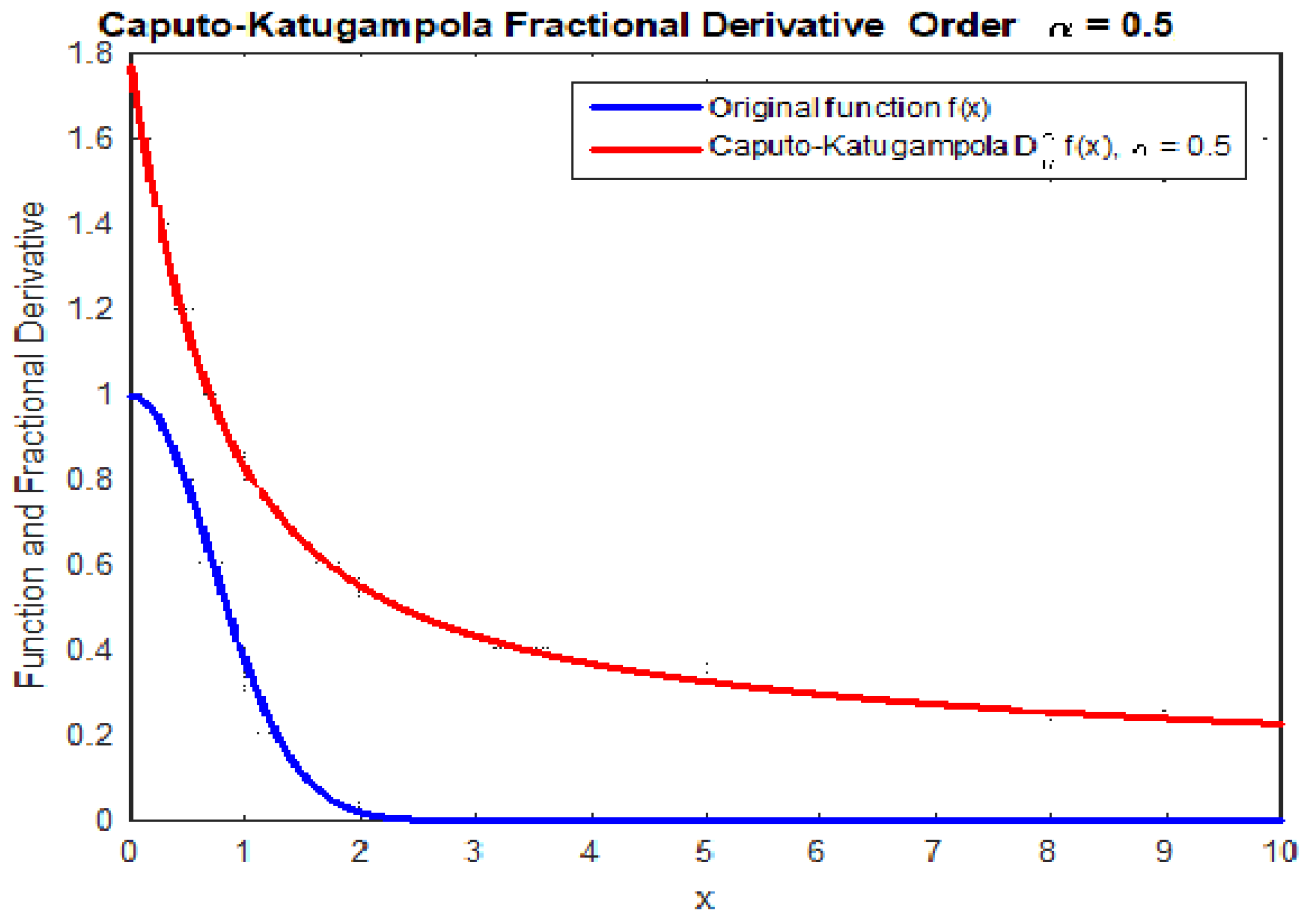
2.2. The Background of the Fractional Differential Equations Tool

The main objective of this section is to present the foundational definitions of fractional differential computing, which are essential for solving our sample models. We introduce the generalized concept of integration, specifically the Riemann integral, which serves as the basis for deriving fractional derivatives. This leads to the well-known definitions of fractional differential calculus, which play a crucial role in specifying solutions to our models. First, we establish the generalized definition of integration, focusing on the Riemann integral as a fundamental tool for extracting fractional derivatives.
Definition 3. 
We define the left Riemann integral of order γ > 0 over a finite interval I = [ m , M ] R of function X ( t ) by its expression
R ( m , t ) ( γ ) X ( t ) = 1 Γ ( γ ) m t ( s t ) γ 1 X ( s ) d s . t > m ,
On the other hand, the right Riemann integral of the same order γ defined by the following expression
R ( t , M ) ( γ ) X ( t ) = 1 Γ ( γ ) t M ( s t ) ( γ ) 1 X ( s ) d s , t < M ,
where  Γ ( γ )  is a Gamma function defined by its expression
Γ ( γ ) = 0 t ( γ ) 1 exp ( t ) d t , Re ( γ ) > 0 . Γ ( γ + 1 ) = ( γ ) Γ ( γ ) if ( γ ) N .
Definition 4. 
The left and right Riemann–Liouville derivatives D ( m , t ) ( γ ) X ( t ) and D ( t , M ) ( γ ) X ( t ) of order ( γ ) are defined by
D ( m , t ) ( γ ) X ( t ) = d N d t N R ( m , t ) ( N γ ) X ( t ) . N = [ ( γ ) ] + 1 .
where
d N d t N R ( m , t ) ( N γ ) X ( t ) . = 1 Γ ( N γ ) d N d t N m t ( t s ) N ( γ ) 1 X ( s ) d s , N N .
Definition 5. 
Additionally, we define the derivative on the right side.
D ( t , M ) ( γ ) X ( t ) = ( 1 ) N d N d t N R ( t , M ) ( N γ ) X ( t ) , N = [ ( γ ) ] + 1 .
where
d N d t N R ( t , M ) ( N γ ) X ( t ) = 1 Γ ( N γ ) d N d t N t M ( s t ) N ( γ ) 1 X ( s ) d s , N N .
It is readily observed that
{ D ( m , t ) N X ( t ) = D ( t , M ) 0 X ( t ) = X ( t ) . D ( m , t ) N X ( t ) = X ( N ) ( t ) . D ( t , M ) N X ( t ) = ( 1 ) N X ( N ) ( t ) .
One of the key motivations for choosing the Caputo derivative is its practical applicability, particularly in fields that rely on realistic modeling, such as physics and economics. In material sciences, the Caputo derivative provides approximations that align well with experimental observations, enabling more accurate predictions of physical behaviors. Similarly, in economics, it supports the dynamic modeling of complex, real-world systems, enhancing the efficiency and relevance of economic analysis and forecasting.
Definition 6. 
The left and right Caputo fractional derivatives are defined as follows, respectively
D ( m , t ) C ( γ ) X ( t ) = 1 Γ ( N γ ) m t X ( N ) ( X ) ( t S ) N γ 1 d S .
where N = [ γ ] + 1 .
D ( t , M ) C ( γ ) X ( t ) = 1 Γ ( N γ ) t M X ( N ) ( X ) ( S t ) N γ 1 d S .
The Hadamard fractional derivative is another type of fractional derivative that differs from the Riemann–Liouville and Caputo derivatives. It is commonly used in applications where the scaling of the derivative changes logarithmically, and it is defined for functions on [ m , M ] such as m > 0 . The Hadamard derivative is particularly useful in fields where logarithmic scaling is natural, such as certain models in biology and finance.
Definition 7. 
We define the Hadamard fractional derivative with order 0 < γ < 1
D ( m , t ) H ( γ ) X ( t ) = 1 Γ ( 1 ( γ ) ) m t ln t s γ X ( s ) d s .
Definition 8. 
A generalized Caputo–Katugampola ( C K ) derivative was proposed by Katugampola in [38,39,40]
D m , t C K ( γ , ε ) X ( t ) = ε ( γ ) Γ ( 1 γ ) m t X ( s ) ( t ε s ε ) γ d s , 0 < γ < 1 ,
It is clear that in the situation where ε tends to 1, we arrive at the Caputo derivative.
Proposition 1. 
The convergence of the two approaches to fractional derivatives holds under the condition that ε tends to zero.
lim ε 0 D m , t C K ( γ , ε ) X ( t ) = D ( m , t ) H ( γ ) X ( t ) .
Proof 
(See [41]). The Caputo–Katugampola fractional derivative is a generalization that unifies and extends various definitions of fractional derivatives, including the Caputo derivative. The key idea behind its limit converging to the standard Caputo derivative lies in the scaling parameter and how the integral kernel behaves as this parameter approaches a certain value. □
Let us denote X ( t n ) : = X n in the following theorems.
Theorem 2. 
Let X : [ a , b ] R be a real C 2 ( [ a , b ] , R ) function. Then, for each positive integer N N , if
D ( t 0 , t ) C K ( α , ε ) X ( t n ) = D ( t 0 , t ) C K ( α , ε ) X n + R ( n ) ,
with the remainder R ( n ) satisfies the following limit:
lim n R ( n ) = 0 .
Then
D ( t 0 , t ) C K ( α , ε ) X n = ε α Γ ( 2 α ) j = 1 n X j X j 1 t j t j 1 t j 1 α t n ε t j ε t n ε 1 1 α t n ε t j ε 1 α .
Proof. 
According to Katugambola’s expression, we have
D ( t 0 , t ) C K ( α , ε ) X ( t ) = ε α Γ ( 1 α ) t t 0 X ( s ) ( t ε s ε ) α d s = ε α Γ ( 1 α ) i = 0 n 1 t i t i + 1 X ( s ) ( t ε s ε ) α s ε 1 s 1 ε d s = ε α Γ ( 1 α ) i = 0 n 1 t i t i + 1 X ( s ) ( t ε s ε ) α s ε 1 s 1 ε d s = ε α Γ ( 1 α ) i = 0 n 1 X i + 1 X i t i + 1 t i t i 1 ε t i t i + 1 s ε 1 ( t ε s ε ) α d s = ε α Γ ( 1 α ) i = 0 n 1 X i + 1 X i t i + 1 t i t i 1 ε ( t ε n t ε i ) 1 α ε ( 1 α ) | t i t i + 1 = ε α Γ ( 1 α ) i = 0 n 1 X i + 1 X i t i + 1 t i t i 1 ε ( t ε n t ε i ) 1 α ( t ε n t ε i + 1 ) 1 α .
The generalized expression proposed in our article is a fractional stochastic differential equation written in the following form:
D CK ( ε , α ) ( t 0 , t ) X ( t ) = γ 0 ( t ) + γ 1 ( t ) X ( t ) + γ 2 ( t ) X ( t ) d W ( t ) ,
We know that the stochastic term d W ( t ) can be numerically approximated using the Euler–Maruyama method, which is the simplest time discretization of the Itô process. Let { X ( t ) } be an Itô process on t [ t 0 , T ] with a classical derivative of order 1, satisfying the stochastic differential equation:
d X ( t ) = γ 0 ( t ) + γ 1 ( t ) X ( t ) d t + γ 2 ( t ) X ( t ) d W ( t ) ,
For a given time discretization
t 0 < t 1 < < t n < t n + 1 ,
the Euler approximation is a continuous-time stochastic process { X ( t ) , t 0 t T } satisfying the following iterative scheme:
Δ X ( t n ) = γ 0 ( t n ) + γ 1 ( t n ) X ( t n ) Δ t n + γ 2 ( t n ) X ( t n ) Δ W ( t n ) ,
for n = 0 , 1 , 2 , , N , with the initial value X ( t 0 ) = X 0 , where
Δ X ( t n ) = X ( t n + 1 ) X ( t n ) , w h e r e , Δ t n = t n + 1 t n ,
In the rules of numerical stochastic calculus, we can approximate the term Δ W ( t n ) according to the following expression, where ξ n is chosen from the standard normal distribution N ( 0 , 1 ) :
Δ W ( t n ) = W ( t n + 1 ) W ( t n ) = ξ n Δ t n .
Then, the model (15) is defined by its recurrent expression:
X ( t n + 1 ) = X ( t n ) + γ 0 ( t n ) + γ 1 ( t n ) X ( t n ) Δ t n + ξ n γ 2 ( t n ) X ( t n ) Δ t n .
Now, we will generalize the stochastic solution by the numerical method of Caputo–Katugampola. First, we will change the model in a way that allows us to approximate it using our specified approach:
D ( t 0 , t ) ( α , ε ) CK X ( t ) = γ 0 ( t ) + X ( t ) γ 1 ( t ) + γ 2 ( t ) d W ( t ) .
Let γ 0 ( t ) = b ( t ) and a ( t ) = { γ 1 ( t ) + γ 2 ( t ) d W ( t ) } . In this case, the model can be written with the simple formula:
D ( t 0 , t ) ( α , ε ) CK X ( t ) = b ( t ) + a ( t ) X ( t ) .
Then, the numerical solution is:
X ( t ) = 1 a ( t ) D ( t 0 , t ) ( α , ε ) CK X ( t ) b ( t ) a ( t ) = 1 a ( t ) ϵ α Γ ( 2 α ) j = 1 n X j X j 1 t j t j 1 t j 1 α t n ϵ t j ϵ 1 α t n ϵ t j ϵ 1 α b ( t ) a ( t ) .
Example 1. 
In neutron scattering theory, the equations governing the space–time evolution and neutron population dynamics are referred to as kinetic equations. These equations are fundamental for understanding the behavior of neutrons in various media, such as nuclear reactors or scattering experiments. To model complex neutron transport phenomena, we consider a generalized form of the neutron flux equation that incorporates a fractional derivative of the Caputo–Katugampola type, which allows for a more accurate representation of memory effects and anomalous diffusion processes in neutron dynamics; see [42]. The following equation is proposed to describe the stochastic motion of neutrons under constrained physical conditions. This equation accounts for the random behavior of neutrons while incorporating specific physical constraints, such as boundary conditions, material properties, or external forces. The proposed stochastic equation takes the form:
D ( 0 , 1 ) C K ( 0.5 , 2 ) X ( t ) = 0.5 X ( t ) + d W ( t ) .
where X ( t ) , 0 = t 0 < t 1 < t 2 = 1 represents the neutron density at time t, measured in units of neutrons per cubic centimeter (neutrons/cm3). To model the stochastic behavior of neutron motion, an approximation of Brownian motion is introduced using a polygonal approximation. This approach discretizes the continuous random motion of neutrons into a series of linear segments, providing a computationally tractable representation of the underlying stochastic process.
W ( t ) = W t i + W t i + 1 W t i t t i t i + 1 t i , t [ 0 , 1 ] .
Then,
X ( t ) = 2 D ( 0 , 1 ) ( 0.5 , 2 ) CK X ( t ) 1 ξ n Δ t n = 2 0.25 Γ ( 3 / 2 ) j = 1 2 X j X j 1 t j t j 1 t j 1 α 1 t j 1 2 0.5 1 t j 2 0.5 1 ξ n Δ t n .

2.3. Foundations and Preliminaries of Bilinear Time-Series Models

Bilinear time-series models represent a significant class of nonlinear models that have proven essential in addressing complex challenges in microeconomics, finance, and beyond. These models enhance traditional linear approaches by incorporating multiplicative interaction terms between past observations and innovations, allowing them to capture intricate nonlinear behaviors such as volatility clustering, asymmetric effects, and regime-dependent dynamics. Historically, the development of bilinear models has been advanced by prominent mathematicians, including Subba Rao, Bibi, and Oyet, who laid the theoretical groundwork for their application. Additionally, these models have been derived through the discretization of stochastic differential equations, further expanding their utility in modeling real-world systems. This section provides a comprehensive foundation for understanding bilinear models and their applications, offering valuable insights to address the specific problem proposed in our paper.
Definition 9. 
The process X ( t ) is defined on a probability space ( Ω , Γ , P ) that satisfies the equation
X ( t ) = k = 1 P α k ( t ) X ( t k ) + k = 1 Q β k ( t ) ε ( t k ) + k = 1 P 0 l = 1 Q 0 γ k l ( t ) X ( t k ) ε ( t l ) + ε ( t ) .
Bilinear models, commonly represented as B L P , Q , P 0 , Q 1 , incorporate time-varying coefficients α k ( t ) , β k ( t ) , γ k l ( t ) and a white-noise component ε ( t ) , which is not necessarily identically distributed and has mean zero and variance σ 2 ( t ) . This white noise can take various forms, such as ARCH, GARCH, or COGARCH in continuous-time processes. In certain cases, ε ( t ) is represented as
ε ( t ) = ξ ( t ) σ ( t ) .
The quantity ( ξ ( t ) ) t Z consists of independent and identically distributed (i.i.d), random variables. Denoting the mathematical expectation by E, it follows that
E ( ξ ( t ) ) = 0 , E ( ξ 3 ( t ) ) = 0 , E ( η 2 ( t ) ) = 1 , E ( η 4 ( t ) ) = m 4 > 0 .
Among the bilinear models studied in terms of existence, the following model is considered
X ( t ) = a ( t ) X ( t 1 ) + b ( t ) X ( t 1 ) ε ( t 1 ) + ε ( t ) .
where a ( t ) and b ( t ) are coefficients with time. Then, the condition of stationarity and model stability (43)
a 2 ( t ) + ε 2 ( t ) b 2 ( t ) < 1 .
In this case, the generalized solution of model (19), using
X ( t ) = j = 1 ε 2 ( t j 1 ) i = 1 j 1 a 2 ( t i N ) + ε 2 ( t i 1 ) b 2 ( t i ) .
We propose a subclass of purely bilinear and strictly superdiagonal processes with periodic coefficients. Given their wide-ranging applications, particularly in economics and finance, bilinear models with time-varying coefficients have emerged as essential tools in the statistical time-series literature, addressing key challenges in modeling complex dynamics. Consider a purely bilinear and strictly superdiagonal model defined by:
X ( t ) = i = 2 N θ i , 1 ( t ) X ( t N ) ε ( t N ) + ε ( t ) , ε ( t ) N ( 0 , σ 2 ( t ) ) .
Let the matrices A and B be of order N × N , with σ 2 ( t ) denoting the variance, and the vectors X t and E of order N × 1 , such that
A = 0 0 0 1 0 0 1 0 0 0 1 0 N × N , B = θ 21 ( b ) θ P 1 ( b ) 0 0 0 0 0 0 0 0 N × N .
Then, defining X ( t ) and E as:
X ( t ) = X ( t ) X ( t 1 ) X ( t N + 1 ) N × 1 , E = 1 X ( t 1 ) X ( t N + 1 ) N × 1 ,
The model can be expressed in vector form:
X ( t ) = ε ( t ) E + A X ( t ) + ε ( t 1 ) B X ( t 1 ) ,
Using the conditions set forth by Bhaskara Rao, Subba Rao, and Walker in [43], it follows that a strictly stationary and ergodic solution to Equation (47) exists if all the eigenvalues of the matrix have moduli less than one.
Γ = A A + σ 2 ( t ) B B .
where ⊗ denotes the Kronecker product of matrices; see [44].
Proposition 2. 
The model defined by Equation (6) admits a unique stationary solution if and only if
σ 2 ( t ) θ 21 2 ( b ) + θ 31 2 ( b ) + + θ P 1 2 ( b ) < 1 ,
For N = 2 , the eigenvalues of Γ are found to be 0 and σ 2 ( t ) b 21 2 ( b ) .
For N = 3 , the eigenvalues of Γ are
σ 2 b 21 2 ( b ) + σ 4 b 21 4 ( b ) + 4 σ 4 b 31 2 ( b ) 2 , σ 2 b 21 2 ( b ) σ 4 b 21 4 ( b ) + 4 σ 4 b 31 2 ( b ) 2 .
Alternatively, the general case of the same type of the bilinear model (19) is considered as follows
X ( t ) = γ 0 ( t ) X ( t q ) + γ 1 ( t ) X ( t q ) ε ( t 1 ) + ε ( t ) .
Under the restriction of the theorem of Klimko and Nilsen in [45], the model can be expressed using the following recursive formulation
X ( t ) = j = 1 i = 1 j 1 γ 0 ( t i q ) + γ 1 ( t i q ) ε ( t i q 1 ) ε ( t j q ) + ε ( t ) ,
Using the expression in [44], the following formula can be extracted
ε ( t ) = X ( t ) a 0 ( t i q ) X ( t q ) j = 1 t 1 ( 1 ) j i = 1 j 1 b 1 ( t i q ) × i = 1 j 1 X ( t i q ) X ( t j ) a 0 ( t i q ) X ( t j q ) .
The process defined by the recurrent series in (46) with the stability condition (49) is bounded. The proof of this theorem is achieved in [2,44]. We revisit the well-known theorem of Klimko and Nilsen, which establishes the existence of estimators and provides the necessary conditions for their validity. We recall the definition of estimator ε ( t ) = X ( t ) p t / t 1 . , where p t / t 1 ( α ) denotes the orthogonal projection, and X ( t ) are the observations X 1 , X 2 , , X N .
Definition 10. 
An ordinary least-squares estimator is any measurable solution of α ^ N , where
α ^ N = arg   min ( Q N ( α ) ) ,
and the penalty function is defined by
Q N ( α ) = 1 N i = 1 N ε t 2 ( α ^ N ) .
For our next theorems, let E denote the mathematical expectation, F t be the σ algebra up to N, and let [ c ] be the integer part of c.
Theorem 3 
([44]). Let X ( t ) , t Z be a stable process generated by (51), where p t / t 1 is almost surely twice continuous in an open subset Ω, containing the true vector α 0 = ( a 0 , b 0 ) of α; let K ,   K 0 be constants, and let α * be a point on the straight line joining α 0 to every α, such as α 0 α < λ . If the following four assumptions are satisfied,
E α 0 2 ε ( t ) γ i 2 4 K , i = 0 , 1 ,
E α 0 2 ε ( t ) γ i γ j E α 0 2 ε ( t ) γ i γ j F t 2 K 0 , i , j = 0 , 1 ,
1 N i = 1 N E α 0 2 ε ( t ) γ i γ j F t converge as sure for matrix M, such as this matrix, which has strictly positive constants,
lim N sup λ 0 1 N λ i = 1 N E α = α 0 2 ε ( t ) γ i γ j E α = α * 2 ε ( t ) γ i γ j < ,
then, there exists an estimator α ^ , where this estimator takes asymptotic behavior such that
α ^ α 0 a s N ,
and
lim N 1 N t = 1 N E α ^ 2 ε ( t ) α 2 ε ( t ) α T t = 1 N E α 0 2 ε ( t ) α 2 ε ( t ) α T 0 .
Proof 
(See [44]). In our approach, we use a demonstration par according to the proposed model in (51). The Klimko and Nilsen theorem can now be proven for time-varying constants, with the proof relying on establishing bounds for p t / t 1 . In this case, to demonstrate that p t / t 1 is bounded, just guarantee that E ( p t / t 1 ) M , where M is a positive constant. We suppose C = max ( ε t n j ) . Then,
E p t / t 1 C j = 1 [ t n ] E i = 1 j 1 E a 0 ( t i n ) + γ 1 ( t i n ) ε ( t i n 1 ) , C j = 1 [ t p ] i = 1 j 1 E γ 0 ( t i n ) + γ 1 ( t i n ) ε ( t i n 1 ) .
Next, apply the Cauchy–Schwarz inequality to obtain
Φ = E γ 0 ( t i n ) + γ 1 ( t i n ) ε ( t i n 1 ) , E γ 0 ( t i n ) + γ 1 ( t i n ) ε ( t i n 1 ) 2 1 2 , E γ 0 2 ( t i n ) + γ 1 2 ( t i n ) ε 2 ( t i n 1 ) 1 2 .
That is to say, we have
E ( ε 2 ( t i n 1 ) ) = σ 2 ( t ) ,
where
γ 0 2 ( t i n ) + γ 1 2 ( t i n ) E ε 2 ( t i n 1 ) 1 2 L < 1 ,
where L is a positive constant.
This proof is obtained from the general expression of the bilinear model (51) and applying the stability condition.
E ( p t / t 1 ) M j = 1 i = 1 j 1 L j = 1 L j 1 .
The Klimko–Nielsen theorem establishes essential conditions for the existence, consistency, and asymptotic normality of maximum likelihood estimators in time-series models. It requires a compact parameter space, correct model specification and compliance with crucial regularity conditions, such as stationarity and ergodicity, to guarantee accurate and reliable estimation.
Definition 11. 
The Autoregressive Conditional Heteroskedasticity (ARCH) model, introduced by Robert Engle (1982) is a statistical model used to describe time-series data where the variance of the error term changes over time. It is particularly useful for modeling financial data, such as stock returns, where ARCH(1) is defined by its following conditional variance
σ 2 ( t ) = a 1 ( t ) + a 2 ( t ) σ 2 ( t 1 ) .
Lemma 1. 
Let the model in (51) driven by ARCH(1) noise and under the following condition
γ 0 ( t i n ) + γ 1 ( t i n ) a 0 ( t ) 1 a 1 ( t ) 1 2 < 1 ,
where 0 a 1 ( t ) < 1 . Then, the series
X ( t ) = ε ( t ) + j = 1 i = 0 j 1 ( γ 0 ( t i n ) + γ 1 ( t i n ) ε t i 1 ) ε t j
is convergent.
Proof. 
Let
X t υ j = 0 t / n 1 i = 0 j 1 ( γ 0 ( t i n ) + ( γ 1 ( t i n ) ε ( t i n 1 ) ,
where υ = max ε ( t i 1 ) , based on the property
E γ 0 ( t i n ) + γ 1 ( t i n ) ε t i n 1 E ( γ 0 ( t i n ) + γ 1 ( t i n ) ε ( t i n 1 ) ) 2 γ 0 ( t i n ) + γ 1 ( t i n ) σ ( t ) , ζ < 1 ,
the result shows that
υ j = 0 t / k 1 ξ j 1 = υ 1 ξ 1 ξ t / n 1 ξ ,
since t approaches , X ( t ) converges to υ ξ ξ 2 . □
Lemma 2. 
Based on [45], if ε ( t ) follows the A R C H ( 1 ) and γ 0 ( t i n ) = 0 in (51), and a 1 ( t ) 0 , 2 e T , where T = 0.5772 , is Euler’s constant; then, when this condition is met
< E ln ( γ 1 ( t i n ) ε ( 1 ) ) < 0 ,
and
X ( t ) = ε ( t ) + j = 1 u = 0 j 1 γ 1 ( t i n ) ε ( t u 1 ) ε ( t j ) ,
Converges almost surely, making X ( t ) the unique strictly stationary solution to the equation.
Theorem 4 
(see [2,44]).  ( ε t ) t Z follows the A R C H ( 1 ) law for the model
X ( t ) = γ 1 ( t n ) X ( t n ) ε ( t 1 ) + ε ( t ) , n N
under the following condition
0 a 1 ( t ) < 1 .
Furthermore, the model guarantees the existence of a unique solution.
Theorem 5. 
If the following condition is met
2 ln γ 1 ( t n ) + ln ( a 0 ( t ) ) ln ( 1 a 1 ( t ) ) < 0 .
Then, the unique strictly stationary solution equation is defined by
X ( t ) = ε ( t ) + j = 1 i = 0 j 1 γ 1 ( t i n ) ε ( t ) ε ( t ) .
The GARCH model will be the next model we talk about. This statistical model is used, particularly in financial markets, to estimate the volatility of time-series data. It is an expansion of the ARCH model, which was created to account for volatility that changes over time and clusters across time.
Definition 12. 
The G A R C H ( 1 , 1 ) model is defined by the white noise, where
ε ( t ) = h ( t ) η ( t ) , η ( t ) N ( 0 , 1 ) h 2 ( t ) = δ 0 ( t ) + α ( t ) ε t 1 2 + β ( t ) h 2 ( t ) .
The sequences α ( t ) and β ( t ) are time-varying coefficients. While δ 0 ( t ) is a positive constant, h ( t ) is independent of the σ field generated by η ( t ) , k 0 , and ε t is a measurable function of the variables η ( t ) , 0 .
Theorem 6. 
GARCH(1,1) model is strictly stationary if and only if
< E log α ( t ) η 2 ( t ) + β ( t ) < 0 .
Proof. 
The proof can be inferred based on the work in ([45]). We propose the same bilinear model as in ([44]), but with white noise from GARCH (1,1).
X t = γ 1 ( t ) X ( t n ) ε ( t ) + ε ( t ) , s 1 ε ( t ) G A R C H ( 1 , 1 ) . .
Some extensions of stability according to the white noise and, recurrently, ε t is written as
ε ( t ) = X ( t ) + k = 1 t 1 ( 1 ) k i = 0 k 1 γ 1 ( t k ) × i = 0 k 1 X ( t i n ) X ( t k ) ,
In the case where
E ( ε t 2 ) = E ( η t 2 ) E ( h t 2 ) = E ( h t 2 ) = γ 0 + α t ( α ) E ( ε t 1 2 ) + β t ( β ) E ( ε t 1 2 ) ,
using the equation E ( ε 2 ( t ) ) = E ( ε 2 ( t 1 ) ) E ( ε t 2 ) , and the necessary condition for model stability
γ 1 ( t ) δ 0 ( t ) 1 α ( t ) β ( t ) < 1 ,
Then,
X ( t ) = ε ( t ) + j = 1 t / n 1 i = 0 j 1 γ 1 ( t i n ) ε ( t i n 1 ) ε ( t n j ) .
The stability of bilinear time-series models plays a crucial role in constructing reliable numerical solutions for fractional stochastic differential equations (FSDEs). By ensuring boundedness and convergence under well-defined conditions (e.g., E [ ln | γ 1 ( t ) ε ( t ) | ] < 0 ), these models preserve the long-term behavior of FSDEs driven by memory effects (Caputo–Katugampola derivatives) and stochastic noise (Brownian motion).
The bilinear structure, with its multiplicative interaction terms X ( t k ) ε ( t l ) , inherently captures nonlinear dependencies while maintaining numerical tractability. Stability guarantees—such as those derived from Klimko–Nilsen theorems or eigenvalue constraints on coefficient matrices—prevent solution divergence, enabling an accurate approximation of fractional dynamics. This property is particularly valuable in nuclear physics and finance, where unstable discretizations could distort memory-dependent phenomena or volatility clustering. Thus, bilinear models provide not just computational efficiency but also a mathematically rigorous foundation for FSDE solutions.

3. Discretization: Key Results and Problem Formulation

The Caputo–Katugampola fractional derivative is a generalization of the Caputo fractional derivative that incorporates an additional parameter, allowing for more flexibility in modeling. The discretization of this operator is essential for numerical simulations and solving fractional differential equations. Below is an outline of the discretization method fo the Caputo–Katugampola fractional derivative. To formulate an expression for approximating the Caputo–Katugampola operator see [46,47,48,49]. The following conditions are proposed. Let I = [ m , M ] , where m > 0 ,   ε > 0 , and n > 0 are a given positive integer where
m = t 0 < t 1 < < t n = M ,
In other ways, we propose the following discretization of the interval I
t = M ( γ ) m ( γ ) n ,
Then,
t s = m ε + s t 1 / ε , s 1 , 2 , , n .
D m , t C K ( γ , ε ) X ( t s ) = ε γ Γ ( 2 γ ) j = 1 s X ( j ) X ( j 1 ) t j t j 1 t j 1 γ t n ε t j 1 ε 1 ( γ ) t n ε t j ε 1 ( γ ) 1 ( γ ) .

Numerical Applications of a Class of Fractional Stochastic Differential Equations

Constructing a numerical solution for a stochastic and fractional equation involves a transformation through discretization, often expressed as a nonlinear time series. Addressing this type of equation in our work necessitates a multidisciplinary approach to ensure an effective formulation. To solve our problem, we relied on insights from the following studies [44,46,50,51] and [28,52,53]: For the following model
D ( t 0 , t ) C K ( θ , r ) X ( t ) = β 0 ( t ) X ( t 1 ) d t + γ 0 ( t ) X ( t 1 ) d W ( t ) .
According to the Caputo–Katugampola (C-K) operator approximation, we have
D ( t 0 , t ) C K ( θ , r ) X ( t n ) = r θ Γ ( 2 ( θ ) ) j = 1 n X ( j ) X ( j 1 ) t j t j 1 × t j 1 θ t n r t j 1 r 1 θ t n r t j r 1 θ .
where X ( t n ) = X ( n ) ; for further explanation, we define
( θ , r , j ) = t j 1 θ t j t j 1 t n r t j 1 r 1 θ t n r t j r 1 θ .
The approximate operator can also be expressed in alternative forms.
D ( t 0 , t ) C K ( θ , r ) X ( t n ) = r θ Γ ( 2 θ ) X ( n ) X ( n 1 ) × ( θ , r , n )
+ j = 1 n 1 ( θ , r , j ) X ( j ) X ( j 1 ) .
We also define the following factor with the following notation
Φ ( ( θ , r , j ) , n 1 ) = j = 1 n 1 ( θ , r , j ) X ( j ) X ( j 1 )
Then,
r θ Γ ( 2 θ ) X ( n ) X ( n 1 ) × ( θ , r , n ) + Φ ( ( θ , r , j ) , n 1 ) = β 0 ( t ) X ( n 1 ) d t + γ 0 ( t ) X ( n 1 ) ε ( t ) .
Recall that d W ( t ) d t = ε ( t ) and c = r θ Γ ( 2 θ ) ; we will obtain
X ( n ) = c X ( n 1 ) × ( θ , r , n ) + Φ ( ( θ , r , j ) , n 1 ) + 1 c β 0 ( t ) X ( n 1 ) d t + γ 0 ( t ) X ( n 1 ) ε ( t ) .

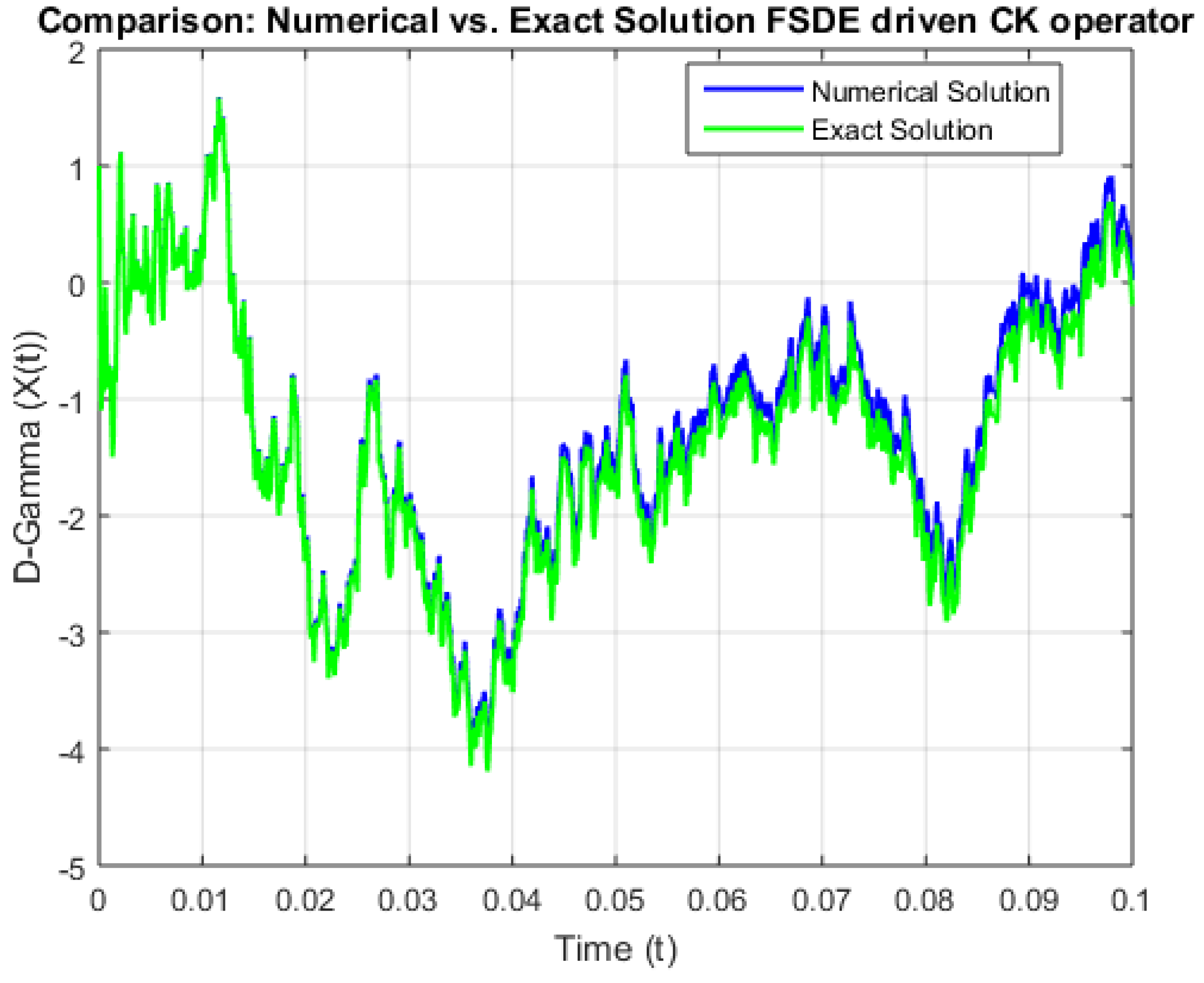
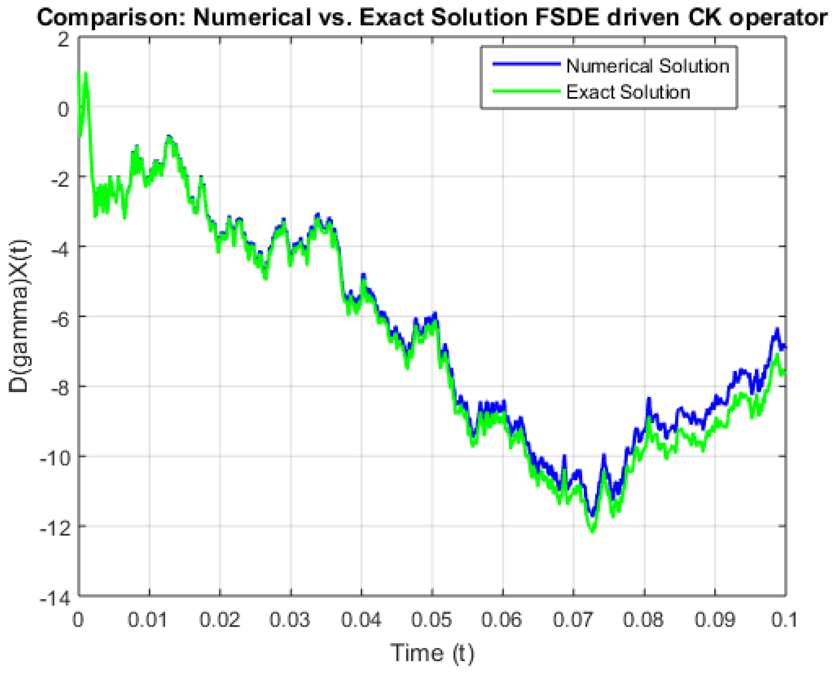
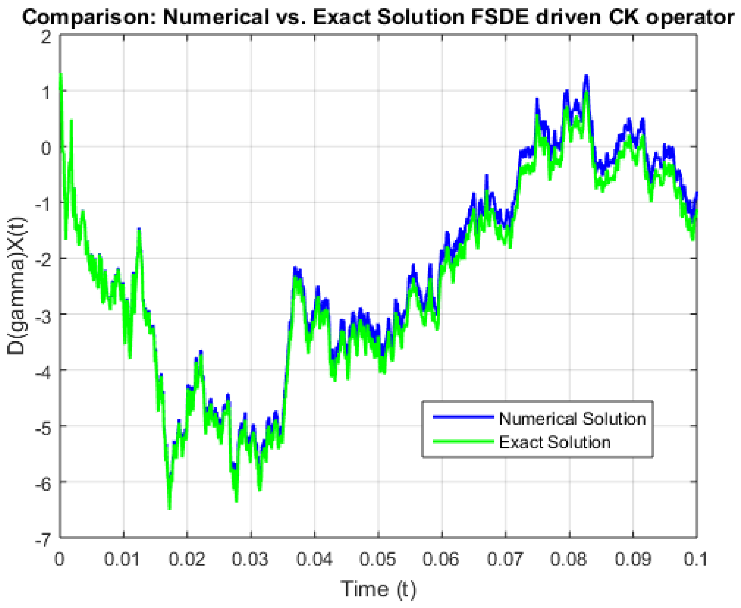
4. Numerical Illustrations and Simulation

This section presents numerical applications to verify the accuracy of the Caputo–Katugampola method in fractional stochastic differential models. We also compare the exact and numerical solutions. We assume that the flux of nuclear energy density is modeled by the following equation:
with X ( 0 ) = 0.01 and 0 < q < 1 . We maintain the same values for the coefficients γ 0 , γ 1 , and γ 2 to facilitate a constructive comparison between the two scenarios. We denote γ i for i = 0 , , 2 as the coefficients, n as the number of subdivisions or sample size, NS for numerical solution, and ES for exact solution. The coefficient values are set as γ 0 = 0.5 , γ 1 = 0.05 , and γ 2 = 0.1 . The Brownian motion example used in the simulation is defined by the expression:
W ( t ) = ε i ( Δ t n ) 0.5 , t [ 0 , 1 ] .
The sequence ( ε i ) i N consists of mutually independent standard Gaussian random variables. Using the polygonal approximation, we define:
w n = w t i + ( w t i + 1 w t i ) t i + 1 t i ( t t i ) , t [ t i , t i + 1 ] .
We can notice in the Table 1 that the increase in the subdivisions (the sample size) gives a better convergence of the numerical solutions toward the exact solution. On the other hand, in the Table 2 , we fix the number of subdivisions, and we have noticed that the raised fractional increase in the expression of Caputo–Katugampola gives a better convergence toward the exact solution. We deduce that the factors of the number of subdivisions and fractional order play a fundamental asymptotic role in the convergence of the numerical solutions by Caputo–Katugampola’s approach. Our future perspectives in this research axis apply frac–stochastic models to the modeling of real physics data and create approaches for this sample of models.
We divide this section into two perspectives; the first is a simple comparison between the exact solution and the numerical solution, and the second is to estimate the coefficients of the fractional stochastic model using transformation to a bilinear model. Our numerical illustration in this paper is to work on a differential stochastic fractional model generated by the following equation using the proposed bilinear time series model.
D ( t 0 , t ) C K ( 0.5 , 1 3 ) X ( t ) = γ X ( t ) d W ( t ) , X ( 0 ) = 0.01
Generate the solution using the following bilinear time series mode
X ( t ) = 0.5 X ( t 1 ) + 0.5 X ( t 1 ) ε ( t 1 ) .
In the following Table 3, we set the number of divisions N = 10.
We observe a convergence between the exact solution and the approximate solution generated by the proposed bilinear model, where the error tends toward zero. This demonstrates that the Katugampola operator plays a fundamental role in the field of approximation, reinforcing its effectiveness in improving numerical solutions.

Some Graphs Representing Convergence

To more precisely measure the convergence, we add some graphs on a smaller interval to detect the convergence between the exact solution and the numerical solution driven by CK method using a bilinear model of the time series with a change in the real model coefficients.
The Figure 1, Figure 2, Figure 3, Figure 4 and Figure 5 compare numerical and exact solutions for a fractional stochastic differential equation (FSDE) driven by a CK operator using with different coefficients of models. All three plots show strong agreement between the numerical and exact solutions over time, validating the discretization method’s accuracy. Notably, graphs highlight the fractional derivative term D(γ)X(t), demonstrating that the numerical scheme preserves key fractional dynamics. Minor deviations may arise from discretization errors or computational constraints, but the overall consistency confirms the robustness of the approach. These results support the method’s reliability for solving FSDEs, making it suitable for broader applications in fractional calculus and stochastic modeling. Further refinement could focus on optimizing computational efficiency for higher-dimensional systems in field of nuclear physics.

5. Conclusions and Future Directions

This study presented a novel approach for solving fractional stochastic differential equations (FSDEs) using a bilinear time-series model, incorporating the Caputo–Katugampola fractional derivative. Through numerical analysis, we observed that increasing the number of subdivisions leads to improved convergence of the approximate solution toward the exact solution. Additionally, the fractional order in the Caputo–Katugampola framework significantly influences the accuracy of numerical solutions, highlighting the fundamental role of fractional operators in modeling memory-dependent stochastic processes. The findings validate the efficiency of this method in capturing complex system dynamics, making it a valuable tool for applications in finance, physics, and engineering. Future work will focus on applying fractional stochastic models to real-world datasets, refining estimation techniques, and further exploring bilinear representations for improved numerical solutions. In future research, we plan to develop and analyze multiple models within this framework, expanding on the theoretical foundations and practical applications of fractional stochastic differential equations. Our focus will be on applying these models to real-world data in finance and economics, allowing us to capture complex market dynamics and economic trends more accurately. By incorporating empirical data, we aim to enhance the relevance and robustness of these mathematical approaches, providing deeper insights into financial modeling, risk assessment, and economic forecasting. This work will contribute to a broader understanding of stochastic processes in applied contexts and demonstrate the practical utility of fractional stochastic differential equations in solving real-world financial and economic challenges, and other future directions include extending this framework to high-dimensional systems and integrating machine learning techniques for adaptive parameter estimation. This work bridges theoretical advancements in fractional calculus with computational practicality, paving the way for broader applications in science and engineering.

Author Contributions

Writing—original draft, commenting, N.L. and M.A.H.; Formal analysis, commenting, Z.C.E.M.; writing—review and editing, B.A.-S.; formal analysis, commenting, funding acquisition, R.A. All authors have read and agreed to the published version of the manuscript.

Funding

This research received no external funding.

Data Availability Statement

The original contributions presented in this study are included in the article material. Further inquiries can be directed to the corresponding author.

Conflicts of Interest

The authors declare no conflicts of interest.

Abbreviations

The following abbreviations are used in this manuscript:
MDPIMultidisciplinary Digital Publishing Institute
DOAJDirectory of open access journals
TLAThree letter acronym
LDLinear dichroism

References

  1. Rothman, P. (Ed.) Nonlinear Time Series Analysis of Economic and Financial Data; Springer: Berlin/Heidelberg, Germany, 2012; Volume 1, pp. 1–300. [Google Scholar]
  2. Rao, T.S.; Gabr, M.M. An Introduction to Bispectral Analysis and Bilinear Time Series Models; Springer: Berlin/Heidelberg, Germany, 2012; Volume 24, pp. 1–224. [Google Scholar]
  3. Almarashi, A.M.; Daniyal, M.; Jamal, F. Modelling the GDP of KSA using linear and non-linear NNAR and hybrid stochastic time series models. PLoS ONE 2024, 19, e0297180. [Google Scholar] [CrossRef] [PubMed]
  4. Evans, L.C. An Introduction to Stochastic Differential Equations; American Mathematical Society: Providence, RI, USA, 2012; Volume 82. [Google Scholar]
  5. Bibi, A.; Merahi, F. GMM Estimation of Continuous-Time Bilinear Processes. Stat. Optim. Inf. Comput. 2021, 9, 990–1009. [Google Scholar] [CrossRef]
  6. Sivalingam, S.M.; Govindaraj, V. A Novel Numerical Approach for Time-Varying Impulsive Fractional Differential Equations Using Theory of Functional Connections and Neural Network. Expert Syst. Appl. 2024, 238, 121750. [Google Scholar]
  7. Sivalingam, S.M.; Kumar, P.; Govindaraj, V. A Novel Method to Approximate Fractional Differential Equations Based on the Theory of Functional Connections. Numer. Algorithms 2024, 95, 527–549. [Google Scholar]
  8. Crauel, H.; Gundlach, M. (Eds.) Stochastic Dynamics; Springer: Berlin/Heidelberg, Germany, 2007. [Google Scholar]
  9. Oksendal, B. Stochastic Differential Equations: An Introduction with Applications; Springer: Berlin/Heidelberg, Germany, 2013. [Google Scholar]
  10. Carriero, A.; Clark, T.E.; Marcellino, M.; Mertens, E. Addressing COVID-19 Outliers in BVARs with Stochastic Volatility. Rev. Econ. Stat. 2024, 106, 1403–1417. [Google Scholar] [CrossRef]
  11. Ma, W.; Jin, M.; Liu, Y.; Xu, X. Empirical Analysis of Fractional Differential Equations Model for Relationship Between Enterprise Management and Financial Performance. Chaos Solitons Fractals 2019, 125, 17–23. [Google Scholar] [CrossRef]
  12. Yavuz, M.; Ozdemir, N.; Okur, Y.Y. Generalized Differential Transform Method for Fractional Partial Differential Equation from Finance. In Proceedings of the International Conference on Fractional Differentiation and its Applications, Novi Sad, Serbia, 18–20 July 2016; Volume 785. [Google Scholar]
  13. Zhang, Z.; Karniadakis, G.E. Numerical Methods for Stochastic Partial Differential Equations with White Noise; Springer: Berlin, Germany, 2017; Volume 196. [Google Scholar]
  14. Ma, L.; Li, C. On Hadamard Fractional Calculus. Fractals 2017, 25, 1750033. [Google Scholar] [CrossRef]
  15. Alzaareer, H.; Al-Zoubi, H.; Al-Mashaleh, W. Classification of Surfaces of Finite Chen II-Type. WSEAS Trans. Math. 2025, 24, 1–7. [Google Scholar] [CrossRef]
  16. Badrakhan, S.; Shaban, E.A.; Oqilat, O.; Taha, J.; Doudeen, H. Efforts Towards Achieving Sustainable Development Goals in Light of National Strategy Jordan’s Vision. J. Educ. Soc. Res. 2024, 16, 1234–1245. [Google Scholar]
  17. Anakira, N.; Almalki, A.; Mohammed, M.J.; Hamad, S.; Oqilat, O.; Amourah, A. Analytical Approaches for Computing Exact Solutions to System of Volterra Integro-Differential Equations. WSEAS Trans. Math. 2024, 23, 400–407. [Google Scholar] [CrossRef]
  18. Kumar, S.; Shaw, P.K.; Abdel-Aty, A.H.; Mahmoud, E.E. A Numerical Study on Fractional Differential Equation with Population Growth Model. Numer. Methods Partial. Differ. Equ. 2024, 40, e22684. [Google Scholar] [CrossRef]
  19. Laiche, N.; Gasmi, L.; Halim, Z. Exploring Novel Approaches for Estimating Fractional Stochastic Processes through Practical Applications. J. Appl. Math. Inform. 2024, 42, 223–235. [Google Scholar]
  20. Almeida, R.; Malinowska, A.B.; Odzijewicz, T. Fractional differential equations with dependence on the Caputo–Katugampola derivative. J. Comput. Nonlinear Dyn. 2016, 11, 061017. [Google Scholar] [CrossRef]
  21. Su, C.-M.; Sun, J.-P.; Zhao, Y.-H. Existence and Uniqueness of Solutions for BVP of Nonlinear Fractional Differential Equation. Int. J. Differ. Equ. 2017, 2017, 4683581. [Google Scholar] [CrossRef]
  22. Sweilam, N.H.; Nagy, A.M.; Al-Ajami, T.M. Numerical Solutions of Fractional Optimal Control with Caputo–Katugampola Derivative. Adv. Differ. Equ. 2021, 2021, 425. [Google Scholar] [CrossRef]
  23. Taroni, M.; Barani, S.; Zaccagnino, D.; Petrillo, G.; Harris, P.A. A Physics-Informed Stochastic Model for Long-Term Correlation of Earthquakes. Preprints 2024. [Google Scholar] [CrossRef]
  24. Liu, W.; Liu, L. Properties of Hadamard Fractional Integral and Its Application. Fractal Fract. 2022, 6, 670. [Google Scholar] [CrossRef]
  25. Liu, J.; Wei, W.; Wang, J.; Xu, W. Limit Behavior of the Solution of Caputo–Hadamard Fractional Stochastic Differential Equations. Appl. Math. Lett. 2023, 140, 108586. [Google Scholar] [CrossRef]
  26. Lin, X.; Zhang, Y.; Wang, H.; Liu, Q. Graph Neural Stochastic Diffusion for Estimating Uncertainty in Node Classification. In Proceedings of the Forty-First International Conference on Machine Learning (ICML), Vienna, Austria, 21–27 July 2024. [Google Scholar]
  27. Zhou, Y. Basic Theory of Fractional Differential Equations; World Scientific: Singapore, 2023. [Google Scholar]
  28. Laiche, N.; Gasmi, L.; Elmezouar, Z.C.; Ozer, O. The Generalized Solution of Fractional Differential Equations Sample with Brownian Motion. Int. J. Nonlinear Anal. Appl. 2024, 15, 361–371. [Google Scholar]
  29. Zhou, Y.; Shangerganesh, L.; Manimaran, J.; Debbouche, A. A Class of Time-Fractional Reaction-Diffusion Equation with Nonlocal Boundary Condition. Math. Methods Appl. Sci. 2018, 41, 2987–2999. [Google Scholar] [CrossRef]
  30. Raubitzek, S.; Mallinger, K.; Neubauer, T. Combining Fractional Derivatives and Machine Learning: A Review. Entropy 2022, 25, 35. [Google Scholar] [CrossRef] [PubMed]
  31. Fukushima, K.; Kamata, S. Stochastic Quantization and Diffusion Models. J. Phys. Soc. Jpn. 2025, 94, 031010. [Google Scholar] [CrossRef]
  32. Poongadan, S.; Lineesh, M.C. Non-Linear Time Series Prediction Using Improved CEEMDAN, SVD and LSTM. Neural Process. Lett. 2024, 56, 164. [Google Scholar] [CrossRef]
  33. Chandrasekhar, S. Stochastic Problems in Physics and Astronomy. Rev. Mod. Phys. 1943, 15, 1. [Google Scholar] [CrossRef]
  34. Bibi, A. The L2–Structure of Subordinated Solution of Continuous-Time Bilinear Time Series. In Time Series Analysis—New Insights; IntechOpen: London, UK, 2022; pp. 1–20. [Google Scholar]
  35. McKean, H.P. Stochastic Integrals; American Mathematical Society: Providence, RI, USA, 2024; Volume 353. [Google Scholar]
  36. Bibi, A.; Merahi, F. Estimating Continuous-Time Bilinear Process with Moments Method. Nonlinear Stud. 2023, 30, 1–15. [Google Scholar]
  37. Cox, S.; Hutzenthaler, M.; Jentzen, A. Local Lipschitz Continuity in the Initial Value and Strong Completeness for Nonlinear Stochastic Differential Equations. Amer. Math. Soc. 2024, 296, 1481. [Google Scholar] [CrossRef]
  38. Al-Ghafri, K.S.; Alabdala, A.T.; Redhwan, S.S.; Bazighifan, O.; Ali, A.H.; Iambor, L.F. Symmetrical Solutions for Non-Local Fractional Integro-Differential Equations via Caputo–Katugampola Derivatives. Symmetry 2023, 15, 662. [Google Scholar] [CrossRef]
  39. Ben Makhlouf, A.; Nagy, A.M. Finite-Time Stability of Linear Caputo-Katugampola Fractional-Order Time Delay Systems. Asian J. Control 2020, 22, 297–306. [Google Scholar] [CrossRef]
  40. Singh, J.; Gupta, A.; Baleanu, D. Fractional Dynamics and Analysis of Coupled Schrödinger-KdV Equation with Caputo-Katugampola Type Memory. J. Comput. Nonlinear Dyn. 2023, 18, 091001. [Google Scholar] [CrossRef]
  41. Kristensen, D. On Stationarity and Ergodicity of the Bilinear Model with Applications to GARCH Models. J. Time Series Anal. 2009, 30, 125–144. [Google Scholar] [CrossRef]
  42. Ray, S.S. Fractional Calculus with Applications for Nuclear Reactor Dynamics; CRC Press: Boca Raton, FL, USA, 2015. [Google Scholar]
  43. Rao, M.B.; Rao, T.S.; Walker, A.M. On the Existence of Some Bilinear Time Series Models. J. Time Series Anal. 1983, 4, 95–110. [Google Scholar] [CrossRef]
  44. Bibi, A.; Oyet, A.J. Estimation of Some Bilinear Time Series Models with Time Varying Coefficients. Stoch. Anal. Appl. 2004, 22, 355–376. [Google Scholar] [CrossRef]
  45. Bibi, A.; Ghezal, A. QMLE of Periodic Time-Varying Bilinear–GARCH Models. Commun. Stat. Theory Methods 2019, 48, 3291–3310. [Google Scholar] [CrossRef]
  46. Zeng, S.; Baleanu, D.; Bai, Y.; Wu, G. Fractional Differential Equations of Caputo-Katugampola Type and Numerical Solutions. Appl. Math. Comput. 2017, 315, 549–554. [Google Scholar] [CrossRef]
  47. Gohar, M.; Li, C.; Li, Z. Finite Difference Methods for Caputo–Hadamard Fractional Differential Equations. Mediterr. J. Math. 2020, 17, 194. [Google Scholar] [CrossRef]
  48. Herrmann, R. Fractional Calculus within the Optical Model Used in Nuclear and Particle Physics. J. Phys. G Nucl. Part. Phys. 2023, 50, 065102. [Google Scholar]
  49. Katugampola, U.N. Existence and Uniqueness Results for a Class of Generalized Fractional Differential Equations. arXiv 2014, arXiv:1411.5229. [Google Scholar]
  50. Fallahgoul, H.A.; Veredas, D.; Fabozzi, F.J. Quantile-Based Inference for Tempered Stable Distributions. Comput. Econ. 2019, 53, 51–83. [Google Scholar] [CrossRef]
  51. Föllmer, H.; Schied, A. Stochastic Finance: An Introduction in Discrete Time; Walter de Gruyter: Berlin, Germany, 2011. [Google Scholar]
  52. Hammad, M.A. Conformable Fractional Martingales and Some Convergence Theorems. Mathematics 2022, 10, 6. [Google Scholar] [CrossRef]
  53. Ghezal, A.; Cavicchioli, M.; Zemmouri, I. On the Existence of Stationary Threshold Bilinear Processes. Stat. Pap. 2024, 1, 1–29. [Google Scholar] [CrossRef]
Figure 1. A comparison between the exact solution and the approximate solution in the Caputo–Katugampola method.
Symmetry 17 00764 g001
Figure 2. Caputo-Katugampola Fractional Derivative Order α = 0.5 .
Symmetry 17 00764 g002
Figure 3. Comparison between exact solution and approximate solution of nuclear physics model of flux with (0.5, 0.5) coefficients with order 0.5.
Symmetry 17 00764 g003
Figure 4. Comparison between exact solution and approximation solution of nuclear physics model of flux with (0.7, 0.7) coefficients with order 0.5.
Symmetry 17 00764 g004
Figure 5. Comparison between exact solution and approximation solution of nuclear physics model of flux with (0.1, 0.9) coefficients with order 0.5.
Symmetry 17 00764 g005
Table 1. Fractional stochastic differential equation density in a nuclear physics (17) model with coefficients.
γ 0 = 0.015 , γ 1 = 0.05 , γ 2 = 0.1
n ( α , ϵ ) ESNS
100 ( 0.5 , 2 ) 0.03450.0396
150 ( 0.5 , 2 ) 0.03450.0351
300 ( 0.5 , 2 ) 0.03450.0339
Table 2. Fractional stochastic differential equation density in a nuclear physics (17) model with coefficients.
γ 0 = 0.015 , γ 1 = 0.05 and γ 2 = 0.1
n ( α , ϵ ) ESNS
1000 ( 0.9 , 2 ) 0.03450.0349
1000 ( 0.5 , 2 ) 0.03450.0377
1000 ( 0.3 , 2 ) 0.03450.0565
Table 3. Comparison between the exact and the approximate solutions.
tExact SolutionApproximative SolutionError
0.100.0475770.0458110.001765
0.200.2610760.2579400.003136
0.300.5677760.5637070.004825
0.400.9448130.9399890.004825
0.501.3808881.3754110.005477
0.601.8688741.8628150.006059
0.702.4037412.3971510.006591
0.902.9816902.9746080.007082
1.003.2659603.1345870.131373
Disclaimer/Publisher’s Note: The statements, opinions and data contained in all publications are solely those of the individual author(s) and contributor(s) and not of MDPI and/or the editor(s). MDPI and/or the editor(s) disclaim responsibility for any injury to people or property resulting from any ideas, methods, instructions or products referred to in the content.

