Abstract
As a new form of economic activity driven by data resources and digital technologies, the digital economy underscores the strategic significance of data as a core production factor. This growing importance necessitates accurate and robust valuation methods. Data valuation poses core modeling challenges due to its nonlinear nature and the instability of neural networks, including gradient vanishing, parameter sensitivity, and slow convergence. To overcome these challenges, this study proposes a genetic algorithm-optimized BP (GA-BP) model, enhancing the efficiency and accuracy of data valuation. The BP neural network employs a symmetrical architecture, with neurons organized in layers and information transmitted symmetrically during both forward and backward propagation. Similarly, the genetic algorithm maintains a symmetric evolutionary process, featuring symmetric operations in both crossover and mutation. The empirical data used in this study are sourced from the Shanghai Data Exchange, comprising 519 data samples. Based on this dataset, the model incorporates 9 primary indicators and 21 secondary indicators to comprehensively assess data value, optimizing network weights and thresholds through the genetic algorithm. Experimental results show that the GA-BP model outperforms the traditional BP network in terms of mean squared error (MSE), root mean squared error (RMSE), mean absolute error (MAE), and coefficient of determination (R2), achieving a 47.6% improvement in prediction accuracy. Furthermore, GA-BP exhibits faster convergence and greater stability. When compared to other models such as long short-term memory (LSTM), convolutional neural networks (CNNs), and optimization-based BP variants like particle swarm optimization BP (PSO-BP) and whale optimization algorithm BP (WOA-BP), GA-BP demonstrates superior generalization and robustness. This approach provides valuable insights into the commercialization of data assets.
1. Introduction
In the era of rapid digital economic growth, data have become a central production factor, profoundly transforming economic growth models and social governance systems. China’s “14th Five-Year Plan for Digital Economy Development” and the “Opinions on Establishing a Data Infrastructure System to Better Leverage the Role of Data Elements” (commonly known as the “Data Twenty Articles”) explicitly highlight the need to accelerate the marketization of data elements and refine data value assessment mechanisms to unlock the economic and social potential of data assets. The core modeling challenge in this process lies in addressing the nonlinearity of data and the sensitivity of neural networks to initial parameters, which complicates the accurate quantification of data’s unstructured value. Moreover, the rapid advancement of artificial intelligence has greatly facilitated the in-depth exploration of data elements, playing a crucial role in data analysis, intelligent forecasting, and value assessment. Despite these advancements, effectively measuring and evaluating the value of data remains a significant challenge in the ongoing process of data marketization.
Existing research on data value assessment primarily follows two approaches. The first approach adapts conventional intangible asset valuation methods—such as the income approach [1], market approach [2], and cost approach [3]—to account for the unique characteristics of data. Wang et al. reviewed current data valuation methodologies, highlighting the importance of incorporating data’s natural increment, externalities, and multidimensional attributes. They also emphasized the need to consider spillover effects in data circulation and evaluate value based on specific application scenarios [4]. Jonathan argued that traditional valuation methods should account for market dynamics as external economic conditions significantly influence data valuation [5]. Xu Xianchun et al. refined the cost approach to improve its applicability in data accounting [6], while Lei et al. enhanced the income approach to increase evaluation accuracy. Among these methods, the cost approach is generally preferred due to its practicality and lower operational complexity, whereas the market and income approaches are more susceptible to external market fluctuations [7]. Yang classified the enterprise data assetization process into three stages—accumulation, application, and assetization—applying the income approach to assess case enterprises [8]. Zhang et al. [9] suggested that the income approach better reflects the profitability of data, yielding results that are widely accepted. Meanwhile, Lu et al. [10] proposed mitigating the limitations of the traditional cost approach by incorporating precise market premium estimations and accurate replacement cost calculations. Lin contended that most studies on traditional valuation methods overlook practical applicability, advocating for the adoption of modern evaluation techniques instead [11].
The second approach to data valuation involves developing specialized derivative models. For instance, Longstaff et al. introduced the least squares Monte Carlo (LSM) model, which integrates least squares regression with the Monte Carlo algorithm for valuation purposes [12]. Zuo et al. proposed replacing the analytic hierarchy process with a multidimensional preference linear programming method to enhance data valuation accuracy [13]. Despite these advancements, no consensus has been reached within the academic community regarding a standardized methodology for data value assessment. Most studies remain anchored in intangible asset valuation frameworks while advocating for the selection of evaluation approaches tailored to the specific attributes of the data [14].
Recent advancements in artificial intelligence have introduced new perspectives on data value assessment. Researchers have increasingly explored the integration of machine learning and deep learning techniques with traditional valuation methods to optimize assessment models and improve predictive accuracy. For example, D. Niyato et al. incorporated the Sternberg model from economics with machine learning classification algorithms to evaluate data utility from a data science perspective [15]. Zhang proposed a deep learning-based model for analyzing both intrinsic and extrinsic data value, validating its effectiveness using production data from port enterprises [16]. Wang et al. developed a fuzzy evaluation model for big data value assessment, employing artificial neural networks to determine indicator weights and applying fuzzy comprehensive evaluation to derive final valuation results [17]. Additionally, Ren constructed a data evaluation system leveraging ensemble machine learning techniques to quantify data value [18]. Wang further highlighted the capability of artificial neural networks to objectively assess data application value, mitigating the subjectivity and variability inherent in manual evaluations [19]. Yan’s research demonstrated that machine learning-based models outperform traditional multiple linear regression methods, with the random forest model exhibiting the highest accuracy in data valuation [20].
Building on these developments, deep learning-based neural network models have gained prominence in data value assessment. Among them, the backpropagation (BP) neural network [21], recognized for its strong nonlinear mapping capabilities and adaptability, has demonstrated significant advantages in data prediction and analysis.
The backpropagation (BP) algorithm has demonstrated significant potential in data valuation applications, particularly in optimizing computational efficiency and enhancing predictive accuracy. For example, Huo et al. [22] implemented a three-layer BP neural network to classify retail stores for fresh food sales forecasting. Their model exhibited accelerated convergence rates and robust resistance to data redundancy and noise during Matlab simulations, achieving superior accuracy in short-term stock price predictions. Further showcasing its versatility, Chen et al. [23] employed BP neural networks during the COVID-19 pandemic to predict user suitability for online education platforms, achieving a classification accuracy of 77.5%. Similarly, Kalinić et al. [24] demonstrated the BP algorithm’s predictive superiority over traditional linear models in analyzing mobile commerce consumer attitudes, highlighting its enhanced ability to capture complex behavioral patterns.
However, traditional BP neural networks exhibit inherent limitations in practical applications, such as a susceptibility to local optima and a hypersensitivity to initial weight-threshold configurations, all of which reduce model stability and predictive reliability. Feng et al. [25] emphasized the algorithm’s critical reliance on initial weights and biases, showing that improper initialization directly degrades valuation accuracy. Deng et al. [26] identified fundamental weaknesses in BP neural networks for elemental prediction in aquatic systems, noting that their tendency toward local minima restricts global optimization potential, thus limiting practical applicability despite satisfactory internal validation performance. To address these limitations, researchers have proposed alternative architectures. For instance, an RBF (radial basis function) neural network model was introduced to overcome the predictive deficiencies of conventional BP networks. Wang et al. [27] systematically analyzed the inherent contradictions between BP’s learning rate and stability, as well as the absence of systematic methods for determining optimal hidden-layer neuron quantities. Similarly, Ye et al. [28] confirmed BP’s convergence instability and structural ambiguity while implementing a modified LM-BP (Levenberg–Marquardt backpropagation) neural network to reduce model error rates through enhanced optimization mechanisms.
To address these challenges, researchers have increasingly integrated metaheuristic optimization algorithms with backpropagation neural networks (BPNNs) in recent years. Notable advancements include hybrid architectures that combine BPNNs with a sparrow search algorithm (SSA) [29], a whale optimization algorithm (WOA) [30], a particle swarm optimization (PSO) [31], and genetic algorithms (GAs) [32]. These integrations enable BPNNs to overcome the constraints of local optima and achieve global optimization capabilities. Among these approaches, the genetic algorithm (GA) has proven particularly effective as a global search mechanism for optimizing the initial weights and thresholds of BPNNs. This GA-BPNN hybridization effectively resolves issues related to instability and local optima entrapment during system training, thereby enhancing both convergence efficiency and predictive performance [33]. When applied to data valuation modeling, the GA-BPNN framework significantly improves prediction efficiency while eliminating the subjective biases inherent in traditional fitting processes, thus enhancing the objectivity and reliability of results [34]. Zhang et al. [35] optimized a BP neural network using an improved genetic algorithm (GA) to model the relationship between weld appearance and molten pool shadow features. Through experiments conducted at welding speeds of 4.5 m/min and 3 m/min, the predictive performance of the model was validated, with the mean absolute percentage error (MAPE) for weld height and width remaining below 4.95%, 4.81%, 5.3%, and 1.4%, respectively. These results demonstrate the model’s high accuracy and stability. Song et al. [36] proposed a BP neural network prediction model integrated with the AdaBoost algorithm to improve prediction accuracy. The average mean absolute error (MAE) decreased from 17,760.1 in the standard BP model to 5,230.6 in the AdaBoost_BP model, representing an approximate 70.5% reduction in error. Liang et al. [37] developed a GA-optimized BP neural network (GA-BP) model to predict the effects of polymer fissure grouting. Compared with the conventional BP model, the GA-BP model improved the coefficient of determination (R2) from 0.975 to 0.991 while reducing MAE by 56.6% and root mean square error (RMSE) by 40.4%, indicating significantly enhanced predictive accuracy and fitting performance. Zhang et al. [38] applied the GA-BP neural network to improve the energy efficiency assessment of crude oil gathering and transportation systems. The GA-BP model increased the R2 for energy utilization efficiency, thermal energy utilization efficiency, and electrical energy utilization efficiency by 1.87%, 0.56%, and 1.37%, respectively. Additionally, the R2 for comprehensive energy consumption, gas consumption, and electricity consumption improved by 2.63%, 0.77%, and 0.31%, respectively, demonstrating that the GA-BP model significantly enhanced prediction accuracy while reducing computational workload. Li et al. [39] employed an interpretable GA-BP strategy to optimize the prediction of interactions at the membrane–sludge particle interface. The mean squared errors (MSEs) for three types of interactions were reduced to 1.0816 × 10⁻⁶, 5.0089 × 10⁻⁹, and 9.0432 × 10⁻⁷, respectively, with the maximum regression coefficient (R) reaching 0.99990 and prediction errors controlled within 0.01%, effectively improving the accuracy of membrane fouling quantification. Li et al. [40], based on construction engineering data from Guangdong Province, proposed a GA-BP model for project cost prediction. The R2 of the testing set increased from 0.87 to 0.94, and the RMSE decreased from 1907.203 to 1281.422, significantly enhancing prediction accuracy and stability.
This study represents the first application of a GA-optimized BP neural network in data value assessment. A comprehensive data value evaluation framework was established based on different “dataset” types, consisting of 9 primary indicators—data quality, data accessibility, data coverage, data diversity, data adaptability, data volume, technical capability, market factors, and data source—and 21 secondary indicators, including producer reputation, supplier qualifications, data quality certification, timeliness, and update speed, among the 21 indicators. The model designed in this study incorporates symmetrical structural features, which contribute to the stability and generalization ability of data value prediction. The GA-BP model effectively optimizes network weights and thresholds, accelerating convergence and improving prediction accuracy while substantially reducing mean squared error (MSE), root mean squared error (RMSE), and mean absolute error (MAE). Simultaneously, it enhances the determination coefficient (R2) [41]. Furthermore, comparative analysis of predicted and actual values, alongside error distribution visualizations, thoroughly validated the advantages of GA-BP in terms of convergence speed, prediction accuracy, and model stability. Experimental results demonstrate that the GA-BP model effectively handles data complexity and heterogeneity, outperforming BP neural networks, long short-term memory (LSTM), convolutional neural networks (CNNs), random forest (RF), support vector machines (SVMs), particle swarm optimization BP (PSO-BP), whale optimization algorithm BP (WOA-BP), and sparrow search algorithm BP (SSA-BP) in both prediction accuracy and model robustness.
2. Materials and Methods
2.1. BP Neural Network
The backpropagation neural network (BPNN) is a multilayer feedforward neural network trained using the error backpropagation algorithm. It consists of an input layer, hidden layers, and an output layer. The BP neural network is characterized by a symmetrical structure where the number of neurons gradually increases and decreases around the hidden layers, forming a symmetric topology. The signal transmission from input to output and the error propagation from output to input also form a symmetrical process. The core principle of a BPNN is to minimize the error between the network’s output and the desired output by adjusting the network’s weights and thresholds through gradient descent. The BP algorithm iteratively optimizes the model through two phases: forward propagation to compute the output and backward propagation to correct the error. It is widely used in classification, regression, and nonlinear modeling tasks [21].
To better illustrate the training process of a BP neural network, we take a three-layer BP neural network structure shown in Figure 1 as an example. The training process of a BP neural network generally consists of two main stages: the forward computation of errors and backpropagation.
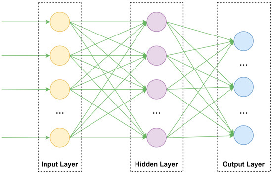
Figure 1.
BP neural network structure.
In the forward computation phase, the output of the hidden layer is first calculated based on the input feature vector . Then, the output layer is computed using . Finally, the prediction error of the BP neural network is determined by comparing the computed output with the expected output . The mathematical formulations for the hidden layer and output layer are given as follows:
where represents the output of the j-th hidden-layer neuron, and are the activation function where is ‘tansig’ for the hidden layer and is ‘purelin’ for the output layer, and denotes the weight between the i-th input neuron and the j-th hidden-layer neuron. corresponds to the input data of the i-th input neuron, while represents the bias term associated with the j-th hidden-layer neuron. Similarly, signifies the output of the k-th output layer neuron, represents the weight between the j-th hidden neuron and the -th output neuron, and denotes the bias term of the -th output neuron.
After obtaining the prediction error of the neural network, the backpropagation phase is initiated to update the weights between the input layer and the hidden layer () and those between the hidden layer and the output layer (), as well as the thresholds of the hidden layer () and the output layer (). The specific process can be expressed as follows:
where was empirically determined to be 0.01 after testing several values (e.g., 0.1, 0.01, 0.001) to ensure model convergence and generalization performance.
During training, forward computation and backpropagation iterate continuously until the MSE requirement is met or the maximum number of epochs is reached. The MSE is propagated back in the form of gradients to adjust the weights and biases of neurons in each layer. The genetic algorithm, inspired by Darwin’s natural selection mechanism, theoretically ensures the continuous optimization of the BP neural network’s weights and biases throughout the training process.
2.2. GA-BP Neural Network
Traditional BP neural networks suffer from slow convergence, a tendency to fall into local optima, and high sensitivity to initial weights and thresholds, all of which significantly impact model stability and prediction accuracy. To address these limitations, genetic algorithms (GAs), known for their efficiency and strong global optimization capabilities, are introduced to optimize the initial parameters of the BP neural network (BPNN). The genetic algorithm (GA) is a global optimization technique inspired by the principles of biological evolution, first proposed by Holland in 1975. Its core mechanism mimics natural selection, crossover, and mutation to explore the solution space and identify optimal solutions. Through iterative population evolution, GA progressively converges toward the global optimum of complex problems, making it particularly suitable for nonlinear, high-dimensional, and multi-modal optimization tasks.
The construction of the GA-BP data value evaluation model can be summarized as follows:
(1) In this study, individuals in the population are encoded using a real number encoding scheme. Each consists of a string of real numbers representing the neuron thresholds and inter-layer connection weights of the BP neural network, forming the initial population. The BPNN is then utilized to predict data value, with the minimization of mean squared error (MSE) on both training and testing sets serving as the fitness function. The fitness of each individual in the initial population is calculated using the following equation:
where and represent the mean squared errors of the training and test sets, respectively; and denote the actual values of the training and test sets; and correspond to the predicted values; and and indicate the number of samples in the training and test sets, respectively. The fitness function, , is a comprehensive measure of the prediction errors on both the training and testing datasets. By minimizing the algorithm optimizes the BP neural network’s fitting ability on the training set and its generalization performance on the testing set, thereby preventing overfitting.
(2) The selection process in the genetic algorithm employs the roulette wheel selection method, where the selection probability of each chromosome is proportional to its fitness. Chromosomes with higher fitness values have a greater likelihood of being selected. The selection probability is calculated using the following equation:
where represents the selection probability of chromosome ; denotes the fitness value of chromosome ; and is the total number of chromosomes in the population.
(3) The crossover operation in the genetic algorithm is performed using a two-point crossover operator. Two crossover points are randomly selected and the gene segments between these points are exchanged. This process can be described as follows: Suppose we have two parent chromosomes, and , represented as follows:
① Randomly selecting crossover points: Two crossover points, and , are randomly chosen such that ;
② Exchanging gene segments: The gene segments between and in the parent chromosomes and are swapped to generate offspring chromosomes.
As a result, the parent chromosomes and exchange gene segments between and , producing the new offspring chromosomes and , which can be represented as follows:
where the gene segments between the crossover points and are exchanged, while the remaining segments remain unchanged.
(4) The mutation operation is carried out using the Gaussian mutation operator, which allows the gene values of an individual to be randomly perturbed within a specified range. This enhances the diversity of the genetic algorithm and improves the convergence quality. The mutation operation for the -th gene of the -th individual is performed as follows:
where represents a Gaussian-distributed random variable with a mean of 0 and a variance of ; denotes the mutation amplitude, which is typically dynamically adjusted during iterations to ensure the algorithm’s balance between global search and local optimization capabilities.
After performing the key operations of roulette wheel selection, two-point crossover, and Gaussian mutation in the genetic algorithm, a new population is generated and the individual fitness values are recalculated according to the fitness function. If the fitness of the optimal individual satisfies the termination condition, this best individual is selected and its corresponding initial weight and threshold values are adopted as the initial parameters for the BP neural network. The optimized BP neural network is then used to train the model, calculate the prediction errors for both the training and testing datasets, and evaluate the model using the mean squared error (MSE). This iterative optimization process continues until the error meets the specified threshold or the maximum number of iterations is reached, at which point the optimal BP neural network model is obtained. It is worth noting that the two-point crossover operator symmetrically exchanges gene segments between parent chromosomes, ensuring a balanced transfer of genetic information and preserving diversity within the solution space. Additionally, Gaussian mutation introduces symmetric perturbations, enabling further exploration of diverse regions in the solution space. These symmetric mechanisms are crucial for maintaining a balance between exploration and exploitation, thereby allowing the genetic algorithm to effectively search for the optimal solution. The flow of the GA-BP algorithm is shown in Figure 2.
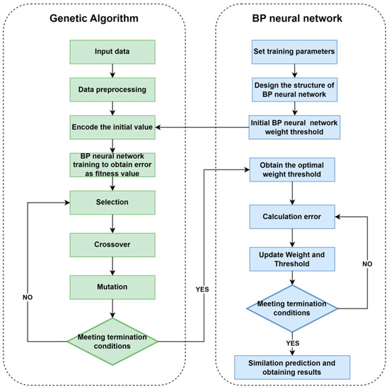
Figure 2.
Flow chart of BP neural network optimized by GA.
2.3. Data Sources and Processing
2.3.1. Data Sources
The data used in this study were sourced from the Shanghai Data Exchange, where it was manually collected, organized, and quantified. Based on the data quality evaluation indicators outlined by the National Information Technology Standardization Technical Committee (GB/T 36344-2018 [42]) and the Data Value Assessment Guidelines (DB61/T 1809-2024 [43]), and further informed by an extensive review of relevant literature in the data industry, the study focuses on data value evaluation, analyzing the key factors influencing data value. Nine primary indicators were identified: data quality, data accessibility, data coverage, data diversity, data adaptability, data volume, technical capability, market factors, and data source. From these, 21 secondary indicators were selected, including producer reputation, supplier qualifications, data quality certification, timeliness, update speed, spatial coverage, scenario coverage, multi-source heterogeneity, application scenario diversity, industry adaptability, data subject relevance, data scale, data increment, data dimensional richness, data update technical capability, functional complexity, pricing model, product type, self-production, open collection, and agreement acquisition. The dataset spans multiple sectors, including financial services, transportation, urban governance, healthcare, trade, industrial manufacturing, technological innovation, modern agriculture, and cultural tourism. To ensure data integrity and accuracy, we conducted data cleaning and deduplication on the original dataset. This process involved removing records with excessive missing values, incorrect formats, or duplicates, ultimately retaining 519 valid data entries. As a result, a data value assessment dataset was constructed, comprising 21 distinct data features, as outlined in Table 1. The sample data are shown in Table 2.

Table 1.
Selection of indicators for the value evaluation model.

Table 2.
Partial sample data.
2.3.2. Correlation Analysis
Correlation analysis is a fundamental technique for feature selection, aiming to quantify the relationship between each feature and the target variable, thereby identifying features that significantly impact the target variable. In high-dimensional datasets some features may be redundant or noisy. Directly incorporating all features can increase computational complexity, exacerbate the curse of dimensionality, and negatively affect the model’s stability and generalization capability. By performing correlation analysis we can effectively eliminate features that contribute little or have no relationship with the target variable, reduce data dimensionality, lower computational costs, and enhance model training efficiency.
In this study, we conducted a correlation analysis between each feature and the overall value to identify key factors influencing data value assessment. Feature selection methods can be categorized into three types: filter methods, wrapper methods, and embedded methods. Considering time efficiency and computational costs, we employed the filter method and used the Pearson correlation coefficient [44] for feature selection. The Pearson correlation coefficient is a widely used statistical metric for measuring the linear relationship between two continuous variables. It quantifies correlation by computing the ratio of the covariance between two variables to the product of their respective standard deviations. The equation is as follows:
where is the Pearson correlation coefficient and the range of is between [−1, 1]; and represent the i-th data points of the variables X and Y, respectively; and and are the means of variables X and Y, respectively.
2.4. Assessment of Model Performance
To evaluate the performance of the GA-BP and BP models, this study employs the mean absolute error (MAE), root mean square error (RMSE), and the coefficient of determination (R2) to assess the prediction performance of each model. The MAE represents the average absolute error between the predicted values and the actual values, indicating the average level of model error. A smaller MAE indicates a smaller deviation between the predicted and actual values, with the unit being CNY (Chinese Yuan). The lower the MAE, the smaller the model’s prediction bias regarding data value, reflecting the accuracy and reliability of the evaluation results. In data value assessment, a smaller MAE signifies that the model can more accurately predict the monetary value of data, thereby assisting decision-makers in better understanding and utilizing data resources. The root mean square error (RMSE) is the square root of the mean squared difference between predicted and actual values, with the unit being CNY (Chinese Yuan). A smaller RMSE indicates better overall model performance with more stable errors, thereby enhancing the reliability of data value assessment. This suggests that the model’s predictions are generally closer to the actual values. The R2 value reflects the degree of correlation between the predicted results and the actual outcomes. A value closer to 1 indicates better model fitting. The formulas for each of these metrics are provided in Equations (18)–(20) and are as follows:
where denotes the actual value of the i-th sample; represents the predicted value of the -th sample; and is the mean of all actual values.
3. Predictive Model Construction
3.1. Data Selection and Normalization
3.1.1. Feature Selection
As shown in Figure 3, by calculating the Pearson correlation coefficient between each feature and the overall value and performing significance testing using p-values, the following features were found to have significant correlation (p < 0.05): X2, X3, X4, X5, X8, X9, X10, X12, X13, X14, and X17. These 11 features with strong correlation were selected as the input parameters.
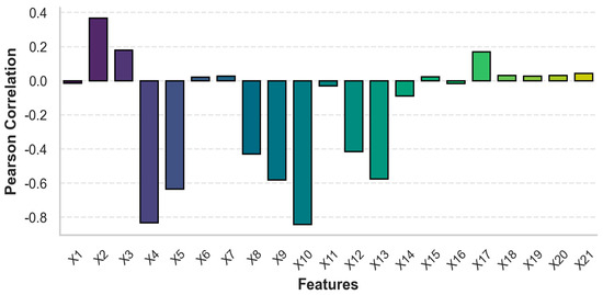
Figure 3.
Pearson correlation coefficient.
3.1.2. Data Processing
(1) The primary objective of data normalization is to eliminate the influence of varying feature scales, ensuring that all data points are distributed within a common range. This process enhances model stability and accelerates convergence. In machine learning and neural network training, significant differences in feature value ranges can slow down optimization and negatively impact model performance. Therefore, normalization is a crucial step in data preprocessing. Common normalization techniques include min–max normalization and Z-score normalization [45], among others. Min–max normalization linearly transforms data into a specified range, improving the model’s adaptability to different features. In this study, the mapminmax function in MATLAB R2022b is employed for data preprocessing and normalization, scaling the data within the range [0, 1]. The transformation equation is as follows:
where represents the standardized data, denotes the original data, is the minimum value of the original data, and is the maximum value of the original data.
(2) The dataset consists of 519 samples, representing transaction records collected between 2022 and 2024. The data are stored in .xlsx format, with each record represented as structured textual data. Of these samples, 70% are randomly selected as the training set. The remaining 30% is evenly divided, with 15% assigned to the test set and 15% to the validation set. This partitioning strategy ensures that the model is trained on a sufficiently large dataset for effective learning while enabling an objective evaluation through independent test and validation sets.
3.2. Backpropagation Neural Networks
In this study, we assessed the performance of neural networks with varying numbers of hidden layers. The results revealed that the three-layer network achieved the highest performance, with an R2 value of 0.90645. Increasing the number of layers resulted in diminished performance: the four-layer network had an R2 of 0.87591 and the five-layer network performed at an R2 of 0.8192. These findings suggest that adding more layers does not yield substantial improvements and may, in fact, reduce the model’s effectiveness. Consequently, we selected the three-layer network as it offers the best balance between model complexity and predictive accuracy. In light of these results, a three-layer BP neural network is constructed using the newff function, and the trainlm function is employed for training. The default Levenberg–Marquardt algorithm [46] is used for optimization as it is well-suited for medium-sized networks that require substantial memory but exhibit fast convergence. Several alternative activation functions were tested, and the combination of tansig and purelin delivered the best performance, achieving an R2 of 0.90645. In comparison, the logsig and purelin combination yielded an R2 of 0.87119 while the tansig–tansig combination resulted in an R2 of 0.88207. The poslin (ReLU) and purelin combination achieved an R2 of 0.90359. Therefore, the transfer function between the input layer and the hidden layer is the tansig S-function, whereas the transfer function between the hidden layer and the output layer is the purelin linear function.
This study initially considers a total of 21 indicators. After feature selection, 11 indicators with significant correlations are retained. Consequently, the number of nodes in the input layer is set to 11. To determine the optimal number of hidden-layer nodes, methods such as the node removal method and the expansion method are commonly used to balance network complexity and error minimization. In this experiment, the trial-and-error approach is adopted; starting with a small number of hidden-layer nodes, the number is gradually increased until the configuration yielding the lowest network error is identified. Additionally, the following empirical formula (Equation (22)) is used to provide an initial estimate for the number of hidden-layer nodes:
where n is the number of nodes in the input layer, s is the number of nodes in the output layer, m is the number of nodes in the hidden layer, and is a constant chosen between [1, 10].
After calculation, the number of nodes in the hidden layer was chosen from the range [4, 13]. Through repeated experiments, as shown in Figure 4, the optimal number of hidden-layer nodes is 8.
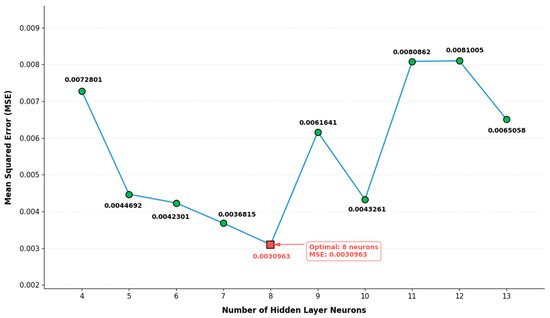
Figure 4.
Impact of different hidden-layer node counts on error.
The output layer consists of a single node, representing the predicted data value. The neural network structure used in this study is illustrated in Figure 5. The final configuration comprises an input layer with 11 nodes, a hidden layer with 8 nodes, and an output layer with 1 node. The specific network parameters are detailed in Table 3.

Figure 5.
Flow chart of BP neural network.

Table 3.
BPNN parameter settings.
3.3. Genetic Algorithm Implementation
In the genetic algorithm, a sensitivity analysis was performed to identify the optimal crossover rate for the genetic algorithm (GA), with a focus on the R2 metric. Crossover rates ranging from 0.5 to 0.9 were evaluated. The results indicated that a crossover rate of 0.7 yielded the highest R2 value of 0.97938, demonstrating the best model performance. In contrast, crossover rates of 0.6, 0.8, and 0.5 produced slightly lower R2 values of 0.97935, 0.97895, and 0.97769, respectively. A crossover rate of 0.9 resulted in a more significant decline, with an R2 value of 0.97395. Accordingly, a crossover rate of 0.7 was selected as the optimal configuration to achieve the highest prediction accuracy. In addition, a mutation rate of 0.2 was selected based on preliminary experiments. This value was found to maintain adequate genetic diversity while preserving convergence stability. Higher mutation rates introduced excessive randomness, which degraded model performance, whereas lower mutation rates led to premature convergence and suboptimal solutions. Therefore, a mutation rate of 0.2 was chosen to achieve an effective balance between exploration and exploitation during the evolutionary process.
Additionally, given the absence of a unified standard for population size, this study adopted a population size of 50 [37]. To validate this selection, population sizes of 5 [47], 20 [38], 30 [34], and 50 [37] were compared based on experimental results. Among these, a size of 50 yielded the highest R2 value (0.97938), while sizes of 20, 30, and 5 produced lower R2 values of 0.97155, 0.96892, and 0.95457, respectively. These results support the choice of a population size of 50 as optimal for achieving superior predictive performance. Therefore, the number of iterations was set to 50. As shown in Figure 6, after the 23rd generation, the individual fitness values no longer changed significantly, indicating that the genetic algorithm had reached a state of convergence.
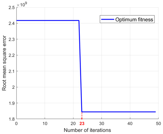
Figure 6.
Individual fitness curve of genetic algorithm.
Ultimately, the selection operator uses the roulette wheel selection method to select individuals with higher fitness. The crossover probability is set to 0.7, and the crossover operator uses two-point crossover. The mutation probability is set to 0.2, with the mutation operator employing Gaussian mutation. After multiple iterations of crossover and mutation the best-fitting individual is obtained and its data become the optimal initial weights and thresholds for the BP neural network. These optimal weights and thresholds are then decoded, and the optimal connection weights between the input layer and the hidden layer, the hidden layer threshold, the connection weights between the hidden layer and the output layer, and the output layer threshold are assigned to the original BP neural network, resulting in the GA-BP neural network. The genetic algorithm is implemented using MATLAB’s built-in ga toolbox, which provides efficient functions for optimization. The parameter settings for the genetic algorithm used in this study are shown in Table 4.

Table 4.
Genetic algorithm parameters.
4. Analysis and Discussion
4.1. BP Neural Network Model Results
Without applying genetic algorithm optimization to initialize the weights and thresholds of the BP neural network, the network was trained directly using the 11 selected correlation features and the parameters from Table 3. The performance of the BP network was then evaluated, yielding the following results. Figure 7 illustrates the variation in the mean squared error (MSE) across training cycles. As training progresses, the MSE gradually decreases and reaches its optimal value at the 10th training cycle, indicating that the BP neural network performs optimally at this point. However, due to the gradient descent method used for weight updates, the BP neural network is prone to becoming trapped in local optima. Figure 8 presents the correlation coefficient (R) of the BP network across the training set, validation set, test set, and overall dataset. As shown in the figure, the correlation coefficient (R) for the test set is 0.96314, while the overall correlation coefficient is 0.97704. These results indicate that most of the predicted values closely align with the training set, though some deviations persist in certain data points. Further analysis reveals that the BP neural network achieves a mean absolute error (MAE) of 63,420.8503 and a coefficient of determination (R2) of 0.90645. While the model can capture the overall data trend its generalization ability remains limited, leaving room for further improvement.
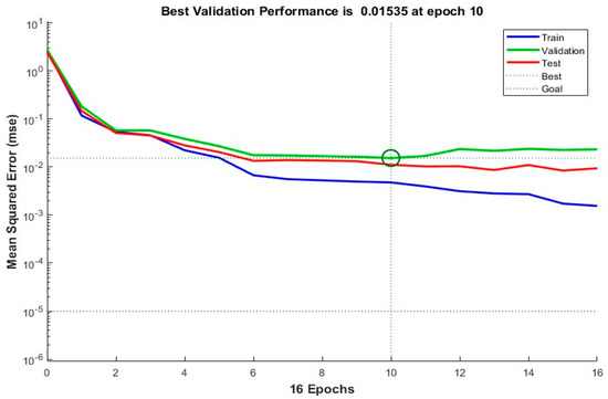
Figure 7.
Network performance of BP model.
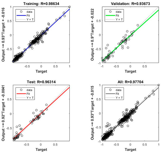
Figure 8.
BP linear regressions of training sets, validation sets, test sets, and the overall data.
4.2. GA-BP Model Results
By applying the genetic algorithm to optimize the BP neural network, the GA-BP model was trained using the 11 selected correlation features and the parameters from Table 4. The results are as follows. Figure 9 illustrates the trend of mean squared error (MSE) during training. As training progresses, the MSE gradually decreases and converges, reaching its optimal value at the 34th training cycle. This indicates that the GA-BP network achieves its best performance at this point. Figure 10 presents the correlation coefficient (R) of the GA-BP model across the training set, validation set, test set, and overall dataset. As shown in the figure, the correlation coefficient (R) for the test set is 0.9915, while the overall correlation coefficient is 0.99288. These values suggest that the GA-BP model maintains consistent performance across different datasets and exhibits strong generalization ability. Furthermore, the GA-BP model achieves a mean absolute error (MAE) of 33,221.7576 and a coefficient of determination (R2) of 0.97938, demonstrating high precision and reliability in data value prediction.
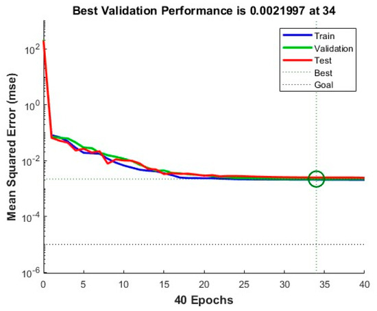
Figure 9.
Network performance of GABP model.
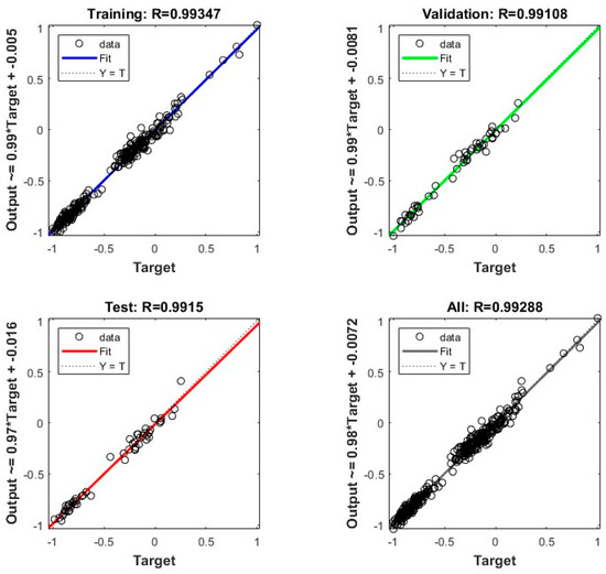
Figure 10.
GABP linear regressions of training sets, validation sets, test sets, and the overall data.
4.3. Model Comparison
4.3.1. Comparison with Other Baseline Models
To assess the effectiveness and superiority of the GA-BP algorithm in data value evaluation, we compared it with LSTM, CNN, RF, and SVM models. The dataset was processed in the same way as for the GA-BP model. The parameter settings for each model are shown in Table 5.

Table 5.
Model Parameter Settings for LSTM, SVM, RF, and CNN.
For each model, a comprehensive hyperparameter tuning process was conducted to optimize performance. To maintain consistency with the GA-BP model, the maximum number of iterations (epochs) and the learning rate were standardized across all models. Specifically, the maximum number of iterations was set to 1000 and the learning rate was set to 0.01 for the LSTM and CNN models.
The remaining hyperparameters for each model were tuned to achieve optimal performance. For the LSTM model, hyperparameters such as the activation function, optimizer, and learning rate decay factor were optimized using grid search. Learning rate decay factors were tested within the range of 0.01 to 0.5, and model performance was evaluated based on validation loss. Additionally, the ReLU activation function and Adam optimizer were selected for their proven effectiveness in training deep learning models. The best combination of these hyperparameters was determined through cross-validation. For the SVM model, a grid search was performed to fine-tune the penalty factor (C) and gamma parameter. The penalty factor was tested between 1.0 and 10.0, while gamma values ranged from 0.1 to 1.0. The optimal parameter combination, which yielded the best classification performance as determined by cross-validation, was selected. This process enhanced the decision boundary and improved the SVM’s ability to generalize to unseen data. For the RF model, the number of decision trees and the minimum number of leaf samples were tuned using random search. The number of trees was tested between 50 and 200, while the minimum number of leaf samples was adjusted between 1 and 10. The goal of the random search was to balance model complexity and accuracy, ensuring the model would not overfit while providing robust predictions on the test data. For the CNN model, we focused on tuning the batch size, learning rate decay factor, and decay period. Using grid search, batch sizes between 16 and 64 and learning rate decay factors between 0.1 and 0.5 were tested. The objective was to minimize training loss and enhance the model’s generalization ability, thereby preventing overfitting and improving predictive performance.
Figure 11, Figure 12, Figure 13, Figure 14, Figure 15 and Figure 16 provide a visual comparison of the predicted and actual values across different models. The results demonstrate that the GA-BP model achieves the highest fitting accuracy, with its prediction curve closely following the 45-degree line indicating strong performance in capturing underlying data patterns. In contrast, the traditional BP model exhibits significant fluctuations, with its curve deviating notably from the 45-degree line, highlighting inconsistent accuracy. The LSTM model shows divergence in some areas, reflecting difficulties in handling the dataset’s complexities and its limited ability to generalize, particularly due to its challenges in modeling non-sequential relationships. The SVM model experiences the largest divergence, with substantial fluctuations from the 45-degree line a result of its sensitivity to data noise and the regularization effect, both of which compromise stability and generalization. The RF model initially fits well but begins to diverge in later stages as it fails to capture long-term dependencies and complex patterns, leading to performance degradation. The CNN model performs reasonably well at first but shows increasing divergence as the predictions progress as its focus on local patterns, typically suited for image data, does not align with the structure of the current dataset, causing accuracy to decline over time.
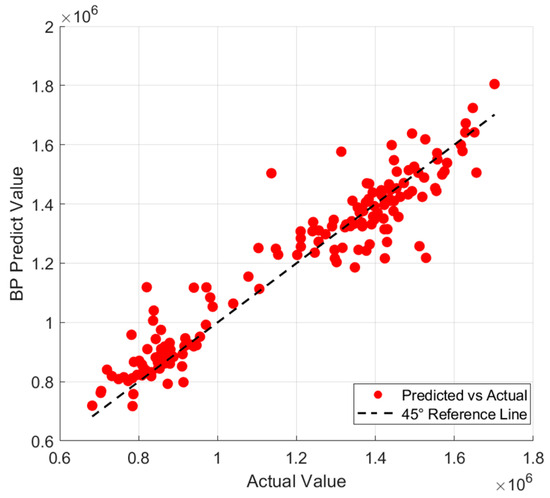
Figure 11.
Comparison of predicted values and true values of BP model.
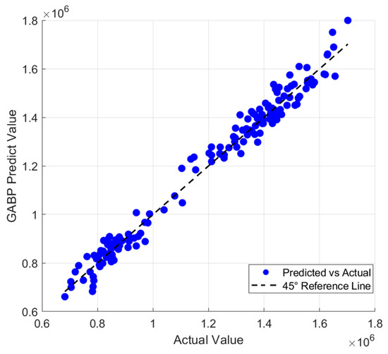
Figure 12.
Comparison of predicted values and true values of GA-BP model.
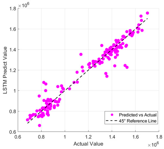
Figure 13.
Comparison of predicted values and true values of LSTM.
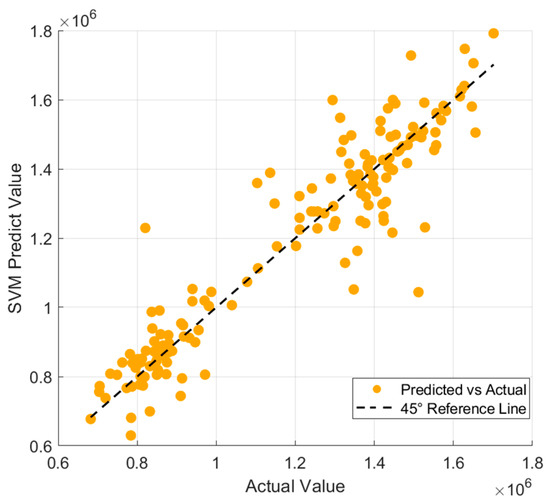
Figure 14.
Comparison of predicted values and true values of SVM.
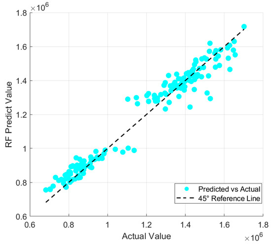
Figure 15.
Comparison of predicted values and true values of RF.
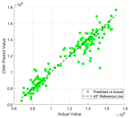
Figure 16.
Comparison of predicted values and true values of CNN.
Figure 17 provides additional validation of the GA-BP model’s superiority. In terms of error distribution, the GA-BP model exhibits significantly lower fluctuation levels than other models, indicating greater stability. The traditional BP model shows the widest error distribution, suggesting weaker generalization capability. The SVM and CNN models display highly dispersed errors, implying greater volatility in prediction accuracy. While the LSTM and RF models maintain relatively stable error distributions, they do not reach the performance level of the GA-BP model. These results highlight the GA-BP model’s distinct advantage in error control, further reinforcing its reliability and precision in data value assessment.
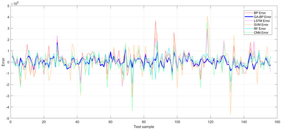
Figure 17.
Error comparison with other foundation models.
As shown in Table 6, the GA-BP model demonstrates significant advantages in prediction error reduction and fitting capability. Compared to other models, GA-BP achieves the lowest MAE and RMSE, reducing these metrics by 23.7% and 28.8%, respectively, relative to the second-best RF model. Additionally, its R2 is the highest, showing a 2.1% improvement over RF, which strongly indicates that GA-BP offers superior prediction accuracy and fitting performance. Among all the compared models the traditional BP neural network performs relatively poorly, with its MAE and RMSE values only marginally better than those of the worst-performing SVM model. After optimization with the genetic algorithm, the GA-BP model improves significantly, reducing the MAE by 47.6%, the RMSE by 53.0%, and increasing the R2 by 8.0%. When compared to deep learning models, GA-BP achieves a 35.7% reduction in MAE compared to LSTM and a 48.1% reduction compared to CNN. Its RMSE is also 49.5% lower than that of LSTM and 55.0% lower than that of CNN. In comparison to other machine learning models, GA-BP reduces RMSE by 60.5% relative to SVM and by 28.8% relative to RF. These results demonstrate that GA-BP effectively mitigates the BP network’s tendency to fall into local optima by leveraging the global search capabilities of the genetic algorithm. Among all the models evaluated in this study, GA-BP exhibits the strongest optimization effect and generalization performance.

Table 6.
Comparison of evaluation metrics for different baseline models.
4.3.2. Comparison with Other Optimization Models
To further evaluate the effectiveness of the genetic algorithm (GA) in optimizing the backpropagation (BP) neural network, this section compares the GA-BP model with other BP-based optimization algorithms, including particle swarm optimization BP (PSO-BP), sparrow search algorithm BP (SSA-BP), and whale optimization algorithm BP (WOA-BP). The dataset used for all models is preprocessed through Pearson correlation analysis to select 11 relevant features. To ensure a fair comparison, the BP network parameters for each optimization algorithm are kept consistent with those listed in Table 3. All comparative experiments employed the same dataset partitioning strategy as the GA-BP model. The population size and maximum number of iterations for SSA-BP, PSO-BP, and WOA-BP were identical to those in GA-BP, both set to 50.
For SSA-BP, three key parameters—population distribution (PD), search space variation (SD), and selection probability (ST)—were optimized. A grid search was employed to assess the impact of varying values for each parameter on convergence speed and accuracy. The PD parameter, affecting population distribution, was tested between 0.3 and 0.5; SD, controlling search space variation, between 0.2 and 0.4; and ST, which influences selection probability, between 0.6 and 0.8. The optimal values were PD = 0.4, SD = 0.3, and ST = 0.7, balancing exploration and exploitation for improved convergence and accuracy while avoiding premature convergence. Similarly, for PSO-BP, the two critical parameters—cognitive learning factor (C1) and social learning factor (C2)—were optimized. These parameters control how particles adjust their positions based on individual experience (C1) and the experience of neighboring particles (C2). A grid search was conducted to evaluate various combinations of C1 and C2 values, both tested in the range of 1.5 to 3.0. After testing several combinations, the optimal values were found to be C1 = 2.0 and C2 = 2.0. These settings facilitated a balanced exploration–exploitation trade-off, leading to faster convergence without compromising the quality of the solution. In contrast, WOA-BP did not require parameter tuning as the whale optimization algorithm (WOA) inherently manages exploration and exploitation through its own mechanism, without the need for user-defined parameters.
Figure 18, Figure 19 and Figure 20 present a visual comparison of the predicted and actual values across different models. The results demonstrate that the GA-BP model achieves the highest fitting accuracy, with its prediction curve aligning more closely with the 45-degree line, reflecting superior performance in capturing underlying data patterns. In contrast, the SSA-BP model shows significant deviations, with some data points moving far from the 45-degree line. This is due to the model’s tendency to become trapped in local optima, impairing its capacity to accurately fit key transitions in the data. The PSO-BP model, although moderately aligned with the 45-degree line, exhibits a moderate level of divergence, reflecting the limited convergence capabilities of particle swarm optimization which results in less refined predictions. The WOA-BP model also displays noticeable deviations, especially at extreme values, as it struggles to capture the full range of data variations, leading to a poor fit at these points. Overall, the GA-BP model consistently demonstrates better alignment with the 45-degree line, ensuring more stable and accurate predictions and effectively addressing the challenges faced by the other models.
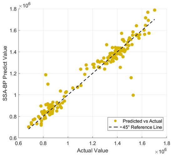
Figure 18.
Comparison of predicted values and true values of SSA-BP model.
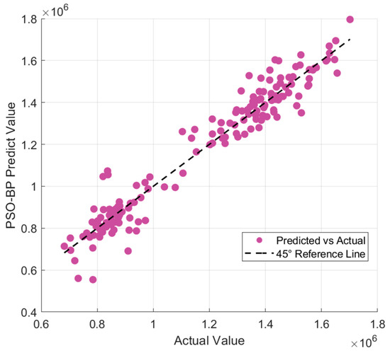
Figure 19.
Comparison of predicted values and true values of PSO-BP model.
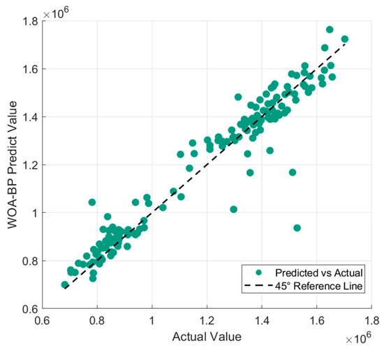
Figure 20.
Comparison of predicted values and true values of WOA-BP model.
Additionally, Figure 21 illustrates that the error fluctuation ranges of the PSO-BP, SSA-BP, and WOA-BP models are significantly larger than that of GA-BP. The prediction errors of PSO-BP exhibit periodic oscillations across samples, while SSA-BP, despite having a lower overall error magnitude, experiences sudden error spikes in highly nonlinear segments, indicating a lack of robustness. WOA-BP, on the other hand, displays the largest error amplitude, with persistent high deviations near extreme points suggesting premature convergence in its parameter optimization process. By contrast, the GA-BP model maintains a consistently low error range, demonstrating significantly improved uniformity and stability in error distribution. These findings quantitatively validate the genetic algorithm’s superiority in neural network optimization.
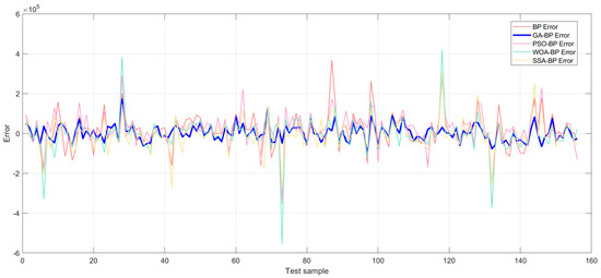
Figure 21.
Error comparison with other optimization algorithms.
Table 7 compares the performance of different optimization models in terms of prediction errors and goodness-of-fit. The SSA-BP model showed improvements across all three metrics—MAE, RMSE, and R2—with MAE decreasing by 17.0%, RMSE by 13.7%, and R2 increasing to 0.9304. In comparison, the PSO-BP model showed limited optimization effects, with MAE reduced by only 6.3%, RMSE improved by 1.3%, and a slight increase in R2 to 0.9089. Although the WOA-BP model reduced MAE by 18.9%, its RMSE increased by 1.4%, and R2 slightly decreased to 0.90385, revealing the instability of its optimization performance. In contrast, the GA-BP model demonstrated notable improvements across all evaluation metrics. MAE was reduced by 47.6%, RMSE improved by 53.0%, and R2 increased to 0.97938, significantly outperforming the other models and highlighting the advantages of the genetic algorithm in neural network optimization.

Table 7.
Comparison of evaluation metrics for different optimization models.
The experimental results indicate that the genetic algorithm, through its global search capability, effectively reduces the BP neural network’s tendency to fall into local optima. Among all the models evaluated, GA-BP showed the best prediction accuracy and model fitting, providing strong support for its application in complex prediction tasks.
4.4. Statistical Analysis of Model Performance
To determine whether the differences in prediction performance between the models are statistically significant an analysis of variance (ANOVA) was conducted. We compared the performance of the following models: the standard BP neural network (BP), the GA-optimized BP neural network (GABP), the SSA-optimized BP (SSA-BP), the PSO-optimized BP (PSO-BP), the WOA-optimized BP (WOA-BP), the long short-term memory (LSTM) network, the support vector machine (SVM), the random forest (RF), and the convolutional neural network (CNN).
The ANOVA results produced an F-statistic of 22.14 and a p-value of 1.77 × 10⁻¹⁷. Since the p-value is well below the commonly accepted significance threshold of 0.05 we reject the null hypothesis, indicating that significant differences exist between the models. This suggests that the GA-optimized BP neural network (GABP) outperforms the other models. To further validate these findings, we conducted a Tukey honest significant difference (HSD) test, which confirmed that GABP shows significant performance differences compared to all other models, with adjusted p-values consistently below 0.05. These results support the conclusion that GA optimization substantially improves the predictive performance of the BP neural network, making GABP the superior model in this comparison.
4.5. Limitations and Future Work
While this study offers valuable insights into data value assessment, several limitations must be acknowledged. First, the relatively small sample size (n = 519) may limit the generalizability of the findings. Second, potential source bias could arise from the exclusive use of data collected from the Shanghai Data Exchange, which may constrain the representativeness of the dataset. Third, the study was conducted within a single country, potentially limiting the applicability of the results across different regulatory, economic, and cultural environments.
Future research should seek to overcome these limitations. Increasing the sample size and incorporating data from multiple exchanges and platforms would enhance the robustness and generalizability of the results. Moreover, cross-national comparative studies are encouraged to validate the model’s applicability in diverse market contexts. Further research could also explore the temporal dynamics of data value evolution and investigate the integration of emerging technologies, such as federated learning and privacy-preserving computation, to further advance the field. Additionally, exploring the use of synthetic data to simulate broader market conditions and test the model’s performance in scenarios where real-world data are limited could provide valuable insights and help in validating the model across diverse, hypothetical market environments.
5. Conclusions
This study introduces a BP neural network model optimized by a genetic algorithm (GA). Through comparative experimental analysis, the results demonstrate that the GA-BP model significantly outperforms traditional BP neural networks in both prediction accuracy and stability. Furthermore, the GA-BP model exhibits clear advantages over popular machine learning models, including long short-term memory (LSTM), convolutional neural networks (CNNs), random forest (RF), and support vector machines (SVMs), as well as optimization algorithms such as particle swarm optimization (PSO), sparrow search algorithm (SSA), and whale optimization algorithm (WOA). These advantages are especially evident when addressing highly nonlinear and complex tasks, such as data value assessment. This is primarily attributed to the effective integration of the genetic algorithm’s global search capability with the BP neural network’s ability to model nonlinear relationships, which collectively overcome the issue of local optima that often hampers traditional BP networks.
In terms of application value, this study contributes significantly beyond simply applying the GA-BP neural network model to the novel field of data value assessment. Specifically, it introduces a new approach by integrating data indicators from various industries to construct a more objective and comprehensive data value assessment model. This approach addresses the subjectivity often found in traditional evaluation methods. The model has potential applications in pricing platforms across sectors such as finance, healthcare, and manufacturing. Furthermore, the study proposes a market-driven valuation method that leverages historical transaction data from multiple sectors, enabling the model to provide intelligent, cross-industry data value assessments. This methodology not only enhances the understanding of data value evaluation but also lays the foundation for a standardized framework that can be applied across different industries. Whilst the study provides valuable insights, limitations such as the relatively small sample size and the data being sourced from a single platform are acknowledged, which may impact the generalizability of the findings.
Future research could expand in several directions. First, in terms of algorithm optimization, further exploration of integrating genetic algorithms with other optimization techniques or incorporating more advanced algorithms could further improve prediction accuracy and generalization ability. Second, in terms of model architecture, the introduction of deep learning techniques, such as attention mechanisms, could enhance feature extraction capabilities. Third, in terms of application expansion, incorporating external factors such as market dynamics and policy environments into the evaluation framework could result in a more comprehensive data value assessment model. Fourth, addressing the current limitations by expanding the sample size, diversifying data sources, synthetic data, and validating the model across multiple countries would enhance its robustness and improve its applicability in international contexts. The GA-BP model proposed in this study offers an effective technical approach for data value assessment. As the digital economy continues to develop, this method is poised to play a significant role in a broader range of data-driven scenarios, supporting the market-based allocation of data resources.
Author Contributions
Conceptualization, X.Q. and X.Y.; methodology, Q.H.; software, Q.H.; validation, X.Q., X.Y. and Q.H.; formal analysis, Q.H.; investigation, Q.H.; resources, X.Q. and X.Z.; data curation, Q.H.; writing—original draft preparation, Q.H.; writing—review and editing, Q.H. and X.Y.; visualization, Q.H.; supervision, X.Q., X.Z. and X.Y.; project administration, X.Q., X.Z. and X.Y.; funding acquisition, X.Q. and X.Z. All authors have read and agreed to the published version of the manuscript.
Funding
This research was funded by the project of the GuangXi Information Center, grant number XZZB202410055F.
Data Availability Statement
The data presented in this study are available on request from the corresponding author. The data are not publicly available due to the project not being completed yet.
Conflicts of Interest
Authors Xujiang Qin and Xin Zhang were employed by the Guangxi Information Center. The remaining authors declare that the research was conducted in the absence of any commercial or financial relationships that could be construed as a potential conflict of interest.
References
- Williamson, O.E. The economics of organization: The transaction cost approach. Am. J. Sociol. 1981, 87, 548–577. [Google Scholar] [CrossRef]
- Han, X.; Wang, S. Attributes, identification and valuation methods of data assets. Stat. Inf. Forum 2023, 38, 3–13. [Google Scholar]
- Baum, A.; Baum, C.M.; Nunnington, N.; Mackmin, D. The Income Approach to Property Valuation; Estates Gazette: London, UK, 2013. [Google Scholar]
- Wang, Y.; Zhao, H. Data asset value assessment literature review and prospect. J. Phys. Conf. Ser. 2020, 1550, 032133. [Google Scholar]
- Jonathan, D. The Data Asset: Databases, Business Intelligence, and Competitive Advantage. Comput. Oper. Res. 1999, 3, 16–24. [Google Scholar]
- Xu, X.; Zhang, Z.; Hu, Y. Research on data asset statistics and accounting issues. Manag. World 2022, 38, 16–30+2. [Google Scholar]
- Lei, X.; Zhang, F. Research on data asset valuation based on the income present value method. Stat. Inf. Forum 2023, 38, 3–13. [Google Scholar]
- Yang, K. Research on enterprise data asset value assessment method. China Manag. Informationization 2022, 25, 88–91. [Google Scholar]
- Zhang, Z.; Tan, C. Research on the value composition and valuation limitations of data assets. Commer. Econ. 2021, 6, 81–82. [Google Scholar]
- Lu, M.; Ouyang, W. Research on the institutional mechanism of data factor marketization and data asset valuation and pricing. Xinjiang Soc. Sci. 2021, 1, 43–53. [Google Scholar]
- Lin, F. Big data assets and their value assessment methods: Literature review and prospects. Financ. Manag. Res. 2020, 6, 1–5. [Google Scholar]
- Longstaff, F.A.; Schwartz, E.S. Valuing American options by simulation: A simple least-squares approach. Rev. Financ. Stud. 2001, 14, 113–147. [Google Scholar] [CrossRef]
- Zuo, W.; Liu, L. Research on big data asset valuation method based on user perceived value. Intell. Theory Pract. 2021, 44, 71–77. [Google Scholar]
- Hu, C.; Li, Y.; Zheng, X. Data assets, information uses, and operational efficiency. Appl. Econ. 2022, 54, 6887–6900. [Google Scholar] [CrossRef]
- Niyato, D.; Alsheikh, M.A.; Wang, P.; Kim, D.I.; Han, Z. Market model and optimal pricing scheme of big data and Internet of Things (IoT). In Proceedings of the 2016 IEEE International Conference on Communications (ICC), Kuala Lumpur, Malaysia, 22–27 May 2016; IEEE: Piscataway, NJ, USA, 2016; pp. 1–6. [Google Scholar]
- Zhang, C. Research on Data Asset Value Analysis Model and Transaction System; Beijing Jiaotong University: Beijing, China, 2018. [Google Scholar]
- Wang, X.; Hao, H.; Zhang, S.; Wang, J. Research on big data value assessment based on fuzzy neural network. Sci. Technol. Manag. 2019, 21, 1–9. [Google Scholar]
- Ren, J. Data asset pricing model and system design based on integrated machine learning. China Manag. Informationization 2022, 25, 80–82. [Google Scholar]
- Wang, J. Research on data asset value evaluation method. Times Financ. 2016, 12, 292–293. [Google Scholar]
- Yan, P. Research on Data Asset Value Assessment Based on Machine Learning; Yunnan University: Kunming, China, 2022. [Google Scholar]
- Li, J.; Cheng, J.H.; Shi, J.Y.; Huang, F. Brief introduction of back propagation (BP) neural network algorithm and its improvement. In Advances in Computer Science and Information Engineering: Volume 2; Springer: Berlin/Heidelberg, Germany, 2012; pp. 553–558. [Google Scholar]
- Huo, L.; Jiang, B.; Ning, T.; Yin, B. A BP neural network predictor model for stock price. In Proceedings of the Intelligent Computing Methodologies: 10th International Conference, ICIC 2014, Taiyuan, China, 3–6 August 2014; Proceedings 10. Springer International Publishing: Cham, Switzerland, 2014; pp. 362–368. [Google Scholar]
- Chen, T.; Peng, L.; Yin, X.; Rong, J.; Yang, J.; Cong, G. Analysis of user satisfaction with online education platforms in China during the COVID-19 pandemic. Healthcare 2020, 8, 200. [Google Scholar] [CrossRef]
- Kalinić, Z.; Marinković, V.; Kalinić, L.; Liébana-Cabanillas, F. Neural network modeling of consumer satisfaction in mobile commerce: An empirical analysis. Expert Syst. Appl. 2021, 175, 114803. [Google Scholar] [CrossRef]
- Feng, W.; Feng, F. Research on the multimodal digital teaching quality data evaluation model based on fuzzy BP neural network. Comput. Intell. Neurosci. 2022, 2022, 7893792. [Google Scholar] [CrossRef]
- Deng, Y.; Zhou, X.; Shen, J.; Xiao, G.; Hong, H.; Lin, H.; Wu, F.; Liao, B.-Q. New methods based on back propagation (BP) and radial basis function (RBF) artificial neural networks (ANNs) for predicting the occurrence of haloketones in tap water. Sci. Total. Environ. 2021, 772, 145534. [Google Scholar] [CrossRef]
- Wang, Y.L.; Liu, Y.; Che, S.B. Research on pattern recognition based on BP neural network. Adv. Mater. Res. 2011, 282, 161–164. [Google Scholar] [CrossRef]
- Ye, Z.; Kim, M.K. Predicting electricity consumption in a building using an optimized back-propagation and Levenberg–Marquardt back-propagation neural network: Case study of a shopping mall in China. Sustain. Cities Soc. 2018, 42, 176–183. [Google Scholar] [CrossRef]
- Xue, J.; Shen, B. A novel swarm intelligence optimization approach: Sparrow search algorithm. Syst. Sci. Control. Eng. 2020, 8, 22–34. [Google Scholar] [CrossRef]
- Mirjalili, S.; Lewis, A. The whale optimization algorithm. Adv. Eng. Softw. 2016, 95, 51–67. [Google Scholar] [CrossRef]
- Wang, D.; Tan, D.; Liu, L. Particle swarm optimization algorithm: An overview. Soft Comput. 2018, 22, 387–408. [Google Scholar] [CrossRef]
- Mirjalili, S. Evolutionary algorithms and neural networks. Stud. Comput. Intell. 2019, 780, 43–55. [Google Scholar]
- Ding, S.; Su, C.; Yu, J. An optimizing BP neural network algorithm based on genetic algorithm. Artif. Intell. Rev. 2011, 36, 153–162. [Google Scholar] [CrossRef]
- Guo, J.; Wu, Q.; Sun, L.; Sheng, H. Lap-slip model of rebar-to-concrete in RC/ECC/UHPC based on GA-BP neural network. Case Stud. Constr. Mater. 2024, 20, e03287. [Google Scholar] [CrossRef]
- Zhang, Y.; Gao, X.; Katayama, S. Weld appearance prediction with BP neural network improved by genetic algorithm during disk laser welding. J. Manuf. Syst. 2015, 34, 53–59. [Google Scholar] [CrossRef]
- Li, S.; Xie, Y.; Wang, W. Application of AdaBoost_BP neural network in prediction of railway freight volumes. Jisuanji Gongcheng Yu Yingyong (Comput. Eng. Appl.) 2012, 48, 6. [Google Scholar]
- Liang, J.; Du, X.; Fang, H.; Li, B.; Wang, N.; Di, D.; Xue, B.; Zhai, K.; Wang, S. Intelligent prediction model of a polymer fracture grouting effect based on a genetic algorithm-optimized back propagation neural network. Tunn. Undergr. Space Technol. 2024, 148, 105781. [Google Scholar] [CrossRef]
- Zhang, X.-Q.; Cheng, Q.-L.; Sun, W.; Zhao, Y.; Li, Z.-M. Research on a TOPSIS energy efficiency evaluation system for crude oil gathering and transportation systems based on a GA-BP neural network. Pet. Sci. 2024, 21, 621–640. [Google Scholar] [CrossRef]
- Li, B.; Shen, L.; Zhao, Y.; Yu, W.; Lin, H.; Chen, C.; Li, Y.; Zeng, Q. Quantification of interfacial interaction related with adhesive membrane fouling by genetic algorithm back propagation (GABP) neural network. J. Colloid Interface Sci. 2023, 640, 110–120. [Google Scholar] [CrossRef] [PubMed]
- Li, C.; Xiao, Y.; Xu, X.; Chen, Z.; Zheng, H.; Zhang, H. Intelligent Forecast Model for Project Cost in Guangdong Province Based on GA-BP Neural Network. Buildings 2024, 14, 3668. [Google Scholar] [CrossRef]
- Chicco, D.; Warrens, M.J.; Jurman, G. The coefficient of determination R-squared is more informative than SMAPE, MAE, MAPE, MSE and RMSE in regression analysis evaluation. PeerJ Comput. Sci. 2021, 7, e623. [Google Scholar] [CrossRef]
- GB/T 36344-2018; Information Technology—Data Quality Evaluation Indicators. Standards Press of China: Shanghai, China, 2018.
- DB61/T 1809-2024; Guidelines for Data Value Assessment. Standards Press of China: Shanghai, China, 2024.
- Cohen, I.; Huang, Y.; Chen, J.; Benesty, J. Pearson correlation coefficient. In Noise Reduction in Speech Processing; Springer: Berlin/Heidelberg, Germany, 2009; pp. 1–4. [Google Scholar]
- Henderi, H.; Wahyuningsih, T.; Rahwanto, E. Comparison of Min-Max normalization and Z-Score Normalization in the K-nearest neighbor (kNN) Algorithm to Test the Accuracy of Types of Breast Cancer. Int. J. Inform. Inf. Syst. 2021, 4, 13–20. [Google Scholar] [CrossRef]
- Moré, J.J. The Levenberg-Marquardt algorithm: Implementation and theory. In Numerical Analysis, Proceedings of the Biennial Conference, Dundee, Scotland, 28 June–1 July 1977; Springer: Berlin/Heidelberg, Germany, 2006; pp. 105–116. [Google Scholar]
- Zhu, C.; Guo, B.; Zhang, Z.; Zhong, P.; Lu, H.; Sigama, A. Determining Rock Joint Peak Shear Strength Based on GA-BP Neural Network Method. Appl. Sci. 2024, 14, 9566. [Google Scholar] [CrossRef]
Disclaimer/Publisher’s Note: The statements, opinions and data contained in all publications are solely those of the individual author(s) and contributor(s) and not of MDPI and/or the editor(s). MDPI and/or the editor(s) disclaim responsibility for any injury to people or property resulting from any ideas, methods, instructions or products referred to in the content. |
© 2025 by the authors. Licensee MDPI, Basel, Switzerland. This article is an open access article distributed under the terms and conditions of the Creative Commons Attribution (CC BY) license (https://creativecommons.org/licenses/by/4.0/).