Analysis Based on a Two-Dimensional Mathematical Model of the Thermo-Stressed State of a Copper Plate During Its Induction Heat Treatment

Abstract

A two-dimensional physical and mathematical model is proposed for determining the components of the stress tensor and stress intensity in an electroconductive plate of rectangular cross-section under the action of an unsteady electromagnetic field. The two-dimensional thermomechanics problem for such a plate is formulated. The determining functions are the component of the magnetic field intensity vector tangent to the plate bases, temperature, and components of the stress tensor. The methodology for solving the formulated thermomechanics problem by approximating all the determining functions by the thickness variable with cubic polynomials is developed. As a result, the original two-dimensional problems related to the determining functions are reduced to one-dimensional problems on the integral characteristics of these functions. To solve the obtained systems of equations for the integral characteristics of the determining functions, a finite integral transformation in the transverse variable is used. During induction heating of a copper plate by a homogeneous quasi-steady-state electromagnetic field, the change in the stress intensity depending on the Fourier time, as well as its distribution across the plate cross-section depending on the parameters of induction heating and the Biot criterion, is numerically analyzed.

1. Introduction

Electroconductive plates, particularly those composed of copper, are widely used as structural elements in electrical engineering devices in the energy sector as current-carrying magnetic cores, in the chemical industry for manufacturing electrolyzers for aluminum smelting, and in the mechanical engineering, automotive, and aerospace industries. The technological heat treatment of copper elements involves the application of external electromagnetic fields (EMFs), particularly quasi-steady ones. Such exposure can affect the mechanical properties of the considered copper elements, as well as their durability and operational reliability.

To describe and investigate electromagnetic, thermal, and mechanical processes in electroconductive elements, appropriate mathematical models, analytical approaches, and experimental methods are used, as outlined in many fundamental studies, including [1,2,3,4,5,6,7]. For describing thermal processes under high-frequency induction heating, relevant physical and mathematical models have been developed in [8,9].

The approach to mixed interpolation of tensor components to study the effect of temperature on nonlinear deflections of shells proposed in [10,11] provides a significant development of the methodology for nonlinear analysis of shell structures under both thermal and mechanical loads. To verify the proposed formulation, the results of finite element analysis are compared with analytical solutions. Based on the results of linear and nonlinear problems, it is shown that the author’s scheme is capable of accurately performing thermomechanical analysis of shell structures.

Paper [12] is devoted to the development of a numerical model and analysis of related electromagnetic and thermal processes in a zone induction heating system for metal billets to determine the optimal ratio of inductor powers and select rational heating modes for billets. For the effective use of induction heating for the heat treatment of electrically conductive elements, it is necessary to provide recommendations for the selection of optimal parameters and heating modes. Accurate calculations of induction heating systems involve taking into account the distribution of the magnetic field, current density, and changes in material properties throughout the volume of the heated workpiece. Work [13] presents the modeling and analysis of electrothermal processes in installations for induction heat treatment of aluminum cores of power cables. This makes it possible to reduce the electrical resistance of the wire and increase its flexibility. In [14], the hybrid microwave melting of lead, tin, aluminum, and copper was experimentally investigated by varying the microwave power level and load. The experimental results were successfully modeled using a lumped parameter model. The results showed that the heat absorption is a strong function of temperature.

Study [15] investigated the temperature and deformation characteristics of a ship hull plate by induction heating using a double-circuit inductor with oppositely directed current. The interconnected electromagnetic-thermal analysis, taking into account the temperature-dependent properties of the material, was iteratively applied at each step of the inductor movement, after which a thermomechanical analysis was performed to obtain the thermal strain, and then it was experimentally confirmed. Paper [16] describes the numerical analysis and experimental study of the triangular induction heating of a rolled sheet. The numerical model used in this study is effective for the steel plate forming process in shipbuilding. The simulation results are compared with the experimental results and show good agreement.

In [17,18], a coupled transient electromagnetic-thermal finite element solution strategy is presented that is suitable for modeling induction heating of both nonferromagnetic and ferromagnetic materials. The solution strategy is based on an isothermal stepwise splitting approach, where the electromagnetic problem is solved for fixed temperature fields and the thermal problem is solved for fixed heat sources obtained from the electromagnetic solution. The modeling strategy and implementation are verified by induction heating experiments at three heating rates. The calculated temperatures are in good agreement with the experimental results.

A mathematical model that accounts for the adiabatic nature of heating and deformation processes under the influence of external pulsed electromagnetic fields with amplitude modulation was proposed in [19] to study the thermo-stressed state of electroconductive bodies. Based on this model, solutions to one-dimensional initial-boundary value problems of thermomechanics for electroconductive bodies of canonical shape have been predominantly obtained, in particular, as in work [20]. However, solutions to two-dimensional initial-boundary value problems remain insufficiently explored.

When one-dimensional models were used, the processes were studied only along the plate thickness or, in the case of a tubular element, along the radial variable. The use of a two-dimensional model for a more complete analysis of the process under study allows us to investigate its change over the cross-sectional area of the plate. This provides a more adequate description of the actual physical process.

2. Materials and Methods

2.1. Two-Dimensional Physical and Mathematical Model of Thermomechanics for an Electroconductive Plate

2.1.1. Initial Positions

We consider an electroconductive plate with a rectangular cross-section, having a thickness of $2d$ and a width of $2d_{\ast }$, in a Cartesian coordinate system $Oxyz$. The origin $O$ coincides with the center of symmetry of the rectangle representing the plate’s cross-section. The Cartesian coordinates $x, y, z$ are referenced to the plate’s half-thickness $h$.

Further, we introduce the dimensionless coordinates $x_1=x/h,x_2=y/h,x_3=z/h$, and define the dimensionless half-width of the plate as $d=d_{\ast }/\mathrm{h}$. The plate’s width is measured along the $O{x}_1$ axis, while it is infinitely long along the $O{x}_2$ axis. The plate’s thickness is measured along the $O{x}_3$ axis.

The plate material is homogeneous, isotropic, and non-ferromagnetic. Its electrical, thermal, and mechanical properties are assumed to be constant and equal to their average values over the corresponding heating intervals.

The induction heating of the plate is carried out by an external uniform quasi-steady electromagnetic field (EMF). As a result of induced currents within the plate, Joule heat is generated, leading to the formation of a transient temperature field, which, in turn, induces a corresponding thermo-stressed state in the plate.

To determine the induced EMF, Joule heat, temperature field, and components of the stress tensor, we consider a two-dimensional physical and mathematical model consisting of three stages.

In the first stage, the EMF and the specific density of Joule heat in the plate are determined based on Maxwell’s equations. In the second stage, the temperature field is obtained from the heat conduction equation, where Joule heat acts as the heat source. Finally, in the third stage, the components of the stress tensor, which describe the thermo-stressed state of the plate, are found by solving the equations of the two-dimensional quasi-static problem of thermoelasticity in terms of stresses.

Thus, the defining functions are the component $H_2\left(x_1,x_3,t\right)$ parallel to the bases $x_3=\pm 1$ and end sections $x_1=\pm d$ of the plate of the magnetic field strength vector $\overrightarrow{H}\left(x_1,x_3,t\right)=\left\{0;H_2\left(x_1,x_3,t\right);0\right\}$; temperature $T\left(x_1,x_3,t\right)$ and components ${\mathsf{\sigma }}_{11},{\mathsf{\sigma }}_{22},{\mathsf{\sigma }}_{33},{\mathsf{\sigma }}_{13}$ of the quasi-static stress tensor ${\mathsf{\sigma }}^{\left(s\right)}$ are different from zero for the plane-deformed state of the plate (here t is the time).

2.1.2. Definition of an Electromagnetic Field

From Maxwell’s relations for the component $H_2\left(x_1,x_3,\mathsf{\tau }\right)$, we obtain the equation:

$${\Delta }_1{H}_2-{\displaystyle \frac{𝜕H_2}{𝜕\tau }}=0.$$

(1)

Here, $\tau =t/\left(\sigma \mu h^2\right)$ is the dimensionless time characteristic of magnetic field diffusion through the half-thickness $h$ of the plate; $\mathsf{\sigma }$ is the electrical conductivity coefficient, $\mu$ is the magnetic permeability of the plate material; ${\Delta }_1={\displaystyle \frac{{𝜕}^2}{𝜕x_1^2}}+{\displaystyle \frac{{𝜕}^2}{𝜕x_3^2}}$ is the Laplace operator.

The action of the external quasi-steady-state EMF is given by the values of the component $H_2\left(x_1,x_3,\mathsf{\tau }\right)$ on all external surfaces of the plate. Therefore, the boundary conditions for solving Equation (1) are:

$$H_2\left(x_1,\pm 1,\tau \right)=H_2^{\pm \left(0\right)}\left(x_1,\tau \right),\hspace{1em}{H}_2\left(\pm d,x_3,\tau \right)=H_2^{\pm \left(0\right)\ast }\left(x_3,\tau \right).$$

(2)

Here, $H_2^{\pm \left(0\right)}\left(x_1,\tau \right)$ and $H_2^{\pm \left(0\right)\ast }\left(x_3,\tau \right)$ are the given expressions of the function on the bases $x_3=\pm 1$ and the end sections of the plate. If at the initial moment of time there is no EMF in the plate, then we obtain a zero initial condition on the function.

Under the uniform action of EMFs at the corner points of the rectangle of the plate cross-section, the conditions for matching the functions $H_2^{\pm \left(0\right)}\left(x_1,\tau \right)$ and $H_2^{\pm \left(0\right)\ast }\left(x_3,\tau \right)$ of the form

$$\begin{gathered} H_2^{+\left(0\right)}\left(d,\tau \right)=H_2^{+\left(0\right)\ast }\left(1,\tau \right);\hspace{1em}{H}_2^{-\left(0\right)}\left(d,\tau \right)=H_2^{\pm \left(0\right)\ast }\left(-1,\tau \right); \\ \hspace{1em}\hspace{1em}\hspace{1em} H_2^{+\left(0\right)}(-d,\tau )=H_2^{-\left(0\right)\ast }(1,\tau );\hspace{1em}{H}_2^{-\left(0\right)}(-d,\tau )=H_2^{-\left(0\right)\ast }(-1,\tau ) \end{gathered}$$

(3)

are fulfilled.

The electric field strength vector $\overrightarrow{E}\left(x_1,x_3,\tau \right)=\left\{E_1\left(x_1,x_3,\tau \right);0;E_3\left(x_1,x_3,\tau \right)\right\}$ in the plate is determined from the relation $\overrightarrow{E}={\displaystyle \frac{1}{\sigma }}$ (rot $\overrightarrow{H}$). Its components are described by the expressions: $E_1={\displaystyle \frac{1}{\sigma }}{\displaystyle \frac{𝜕H_2(x_1,x_3,\tau )}{𝜕x_1}}$, $E_3=-{\displaystyle \frac{1}{\sigma }}{\displaystyle \frac{𝜕H_2(x_1,x_3,\tau )}{𝜕x_3}}$. The specific heat density of Joule is found by the formula

$$Q={\displaystyle \frac{1}{\sigma }}\left[{\left({\displaystyle \frac{𝜕H_2}{𝜕x_1}}\right)}^2+{\left({\displaystyle \frac{𝜕H_2}{𝜕x_3}}\right)}^2\right].$$

(4)

2.1.3. Definition of the Temperature Field

The temperature field $T\left(x_1,x_3,t\right)$ in the plate, which is due to Joule heat $Q$, is determined from the heat conduction equation:

$${\Delta }_{1}T-{\displaystyle \frac{𝜕T}{𝜕Fo}}={\displaystyle \frac{-h^2}{\lambda }}Q.$$

(5)

Here, $Fo=at/h^2$ is the Fourier time; a and λ are the temperature and thermal conductivity coefficients.

We assume that on the surfaces $x_3=\pm 1$ the conditions of convective heat transfer

$${{\displaystyle \frac{𝜕T}{𝜕x_3}}}^{\pm }\pm B{i}^{\pm }(T^{\pm }-T_c^{\pm })=0$$

(6)

hold with the external environment, where the temperatures of the external medium at the surfaces $x_3=\pm 1$ of the plate are equal to $T_c^{\pm }$. Here $B{i}^{\pm }=H^{\pm }h$ is Biot criterion; $H^{\pm }$ is the relative heat transfer coefficient; $T^{\pm }$ and ${\left({\displaystyle \frac{𝜕T}{𝜕x_3}}\right)}^{\pm }$ are the values of the temperature and its derivative at the bases $x_3=\pm 1$ of the plate.

2.1.4. Definition of Thermally Stressed State

From previous studies [21,22], it is known that during the induction heating of an electroconductive body by a quasi-steady-state EMF, the stress state of this body is mainly determined by the Joule heat $Q$, and the influence of the ponderomotive forces $\overrightarrow{F}$ is negligible. Therefore, in the case of a plane deformation of the plate caused only by the temperature field $T\left(x_1,x_3,t\right)$, the components ${\mathsf{\sigma }}_{11},{\mathsf{\sigma }}_{22},{\mathsf{\sigma }}_{33},{\mathsf{\sigma }}_{13}$ of the quasi-static stress tensor ${\widehat{\mathsf{\sigma }}}^{\left(s\right)}$ are determined from the system of equations of the two-dimensional quasi-static thermoelasticity problem in stresses. This system in the dimensional Cartesian coordinates $x_1=x, x_2=y, x_3=z$ has the form [23,24]

$$\begin{gathered} \hspace{1em}\hspace{1em}{\Delta }_1\left({\psi }^{\left(s\right)}+{\displaystyle \frac{\alpha ET}{1-\nu }}\right)=0,\hspace{1em}{\Delta }_1{\sigma }_{13}^{\left(s\right)}=-{\displaystyle \frac{{𝜕}^2{\psi }^{\left(s\right)}}{𝜕x_1𝜕x_3}},\hspace{1em}{\displaystyle \frac{𝜕{\sigma }_{11}^{\left(s\right)}}{𝜕x_1}}={\displaystyle \frac{𝜕{\sigma }_{13}^{\left(s\right)}}{𝜕x_3}}, \\ {\sigma }_{33}^{\left(s\right)}={\psi }^{\left(s\right)}-{\sigma }_{11}^{(s\_)},\hspace{1em}{\sigma }_{22}^{\left(s\right)}=\nu {\psi }^{\left(s\right)}-\alpha ET. \end{gathered}$$

(7)

Here, $\alpha , \nu$ are the coefficients of linear thermal expansion and Poisson’s ratio; $E$ is Young’s modulus; ${\psi }^{\left(s\right)}={\sigma }_{11}^{(s\_)}+{\sigma }_{33}^{\left(s\right)}$.

The boundary conditions on the bases $x_3=\pm h$ of the plate are as follows

$${\displaystyle \frac{𝜕{\psi }^{\left(s\right)\pm }}{𝜕x_1}}+{\displaystyle \frac{𝜕{\sigma }_{13}^{\left(s\right)\pm }}{𝜕x_3}}=0,\hspace{1em}{\displaystyle \frac{𝜕{\sigma }_{13}^{\left(s\right)\pm }}{𝜕x_3}}=0,\hspace{1em}{\sigma }_{11}^{\left(s\right)\pm }={\psi }^{\left(s\right)\pm },$$

(8)

and on the end surfaces $x_1=\pm d$ of the plate these conditions are written

$${\displaystyle \frac{𝜕{\psi }_{\ast }^{\left(s\right)\pm }}{𝜕x_3}}+{\displaystyle \frac{𝜕{\sigma }_{\ast 13}^{\left(s\right)\pm }}{𝜕x_1}}=0,\hspace{1em}{\sigma }_{\ast 13}^{\left(s\right)\pm }=0,\hspace{1em}{\sigma }_{\ast 33}^{\left(s\right)\pm }={{\psi }_{\ast }}^{\left(s\right)\pm }.$$

(9)

The symbol * in Formula (9) means that these values are considered at the end sections $x_1=\pm d$ of the plate.

2.2. Methodology for Constructing Solutions to Two-Dimensional Initial Boundary Value Problems

To find the determining functions $\mathsf{\Phi }=\{H_2\left(x_1,x_3,t\right);T\left(x_1,x_3,t\right);{\mathsf{\sigma }}_{11}\left(x_1,x_3,t\right);{\mathsf{\sigma }}_{13}\left(x_1,x_3,t\right);{\mathsf{\sigma }}_{22}\left(x_1,x_3,t\right);{\mathsf{\sigma }}_{33}\left(x_1,x_3,t\right)\}$ we approximate their distribution over the thickness variable $x_3$ by cubic polynomials [25]

$$\mathsf{\Phi }\left(x_1,x_3,t\right)={\sum }_{j=1}^3{a}_{\left(j-1\right)}^{\mathsf{\Phi }}\left(x_1,t\right)x_3^{j-1}.$$

(10)

The coefficients $a_{\left(j-1\right)}^{\Phi }\left(x_1,t\right)$ of the approximation polynomials (10) were written through the integral characteristics ${\Phi }_s\left(x_1,t\right)$ of the determining functions $\mathsf{\Phi }\left(x_1,x_3,t\right)$

$$\mathsf{\Phi }\left(x_1,t\right)={\displaystyle \frac{2s-1}{2}}{\int }_{-1}^1\mathsf{\Phi }\left(x_l,x_3,t\right)x_3^{s-1}d{x}_3,\hspace{1em}\left(s=1, 2\right)$$

(11)

and the boundary values ${\Phi }^{\pm }\left(x_1,t\right)$ of these functions on the bases $x_3=\pm h$ of the plate. The equation for determining the integral characteristics ${\mathsf{\Phi }}_{\mathrm{s}}\left(x_1,t\right)$ is obtained by multiplying Equations (1), (5), and (7) by $x_3^{s-1}$ and integrating them over the variable $x_3$, taking into account Formulas (10) and (11).

The resulting systems of initial equations for finding the integral characteristics ${\mathsf{\Phi }}_{\mathrm{s}}\left(x_1,t\right)$ $\left(s=1, 2\right)$ of the determining functions will be systems of one-dimensional equations in the spatial variable $x_1$.

To find their solutions, we use finite integral transformations [26] in the variable $x_1$ in accordance with the boundary conditions set on the defining functions at the end sections $x_1=\pm d$ of the plate under consideration. Note that the integral characteristics $H_{2s}$ of the component $H_2\left(x_1,x_3,\tau \right)$ of the magnetic field intensity vector and temperature $T_s$ are also determined using the Laplace integral transform with respect to the dimensionless time variables $\tau$ and $Fo$. The procedure for determining the components of the magnetic field intensity and temperature vector is described in [27].

To construct the solution of the considered quasi-static problem of thermoelasticity described by the relations (7)–(9) for the plate, let us approximate the distribution of the functions ${\psi }^{\left(s\right)}(x_1,x_3)$ and ${\sigma }_{13}^{\left(s\right)}(x_1,x_3)$ along the thickness coordinate $x_3$ by cubic polynomials

$${\psi }^{\left(s\right)}=\sum _{j=1}^4{\psi }_{j-1}^{\left(s\right)}(x_1)x_3^{j-1}.$$

(12)

$${\sigma }_{13}^{\left(s\right)}=\sum _{j=1}^4{\alpha }_{13(j-1)}^{\left(s\right)}(x_1)x_3^{j-1}.$$

(13)

Then, the coefficients ${\psi }_{j-1}^{\left(s\right)},{\alpha }_{13(j-1)}^{\left(s\right)}$ of the approximation polynomials are expressed in terms of integral characteristics

$$\begin{array}{l}{N}^{\left(s\right)}={\displaystyle \frac{1}{2h}}{\int }_{-h}^h{\psi }^{\left(s\right)}d{x}_3;\hspace{1em} M^{\left(s\right)}={\displaystyle \frac{3}{2h^2}}{\int }_{-h}^h{\psi }^{\left(s\right)}{x}_{3}d{x}_3;\\ N_{13}^{\left(s\right)}={\displaystyle \frac{1}{2h}}{\int }_{-h}^h{\sigma }_{13}^{\left(s\right)}d{x}_3;\hspace{1em}{M}_{13}^{\left(s\right)}={\displaystyle \frac{3}{2h^2}}{\int }_{-h}^h{\sigma }_{13}^{\left(s\right)}{x}_{3}d{x}_3.\end{array}$$

(14)

of the functions ${\psi }^{\left(s\right)}(x_1,x_3)$ and ${\sigma }_{13}^{\left(s\right)}(x_1,x_3)$ on the thickness coordinate $x_3$ and the boundary values of these functions as follows

$$\begin{array}{l}{\psi }_{\left(0\right)}^{\left(s\right)}={\displaystyle \frac{3}{2}}{N}^{\left(s\right)}-{\displaystyle \frac{1}{4}}{\psi }_{\ast }^{\left(s\right)};\hspace{1em}{\psi }_{\left(1\right)}^{\left(s\right)}={\displaystyle \frac{5}{2h}}{M}^{\left(s\right)}-{\displaystyle \frac{3}{4h}}{\psi }_{\ast \ast }^{\left(s\right)};\hspace{1em}\\ {\psi }_{\left(2\right)}^{\left(s\right)}={\displaystyle \frac{3}{4h^2}}{\psi }_{\ast }^{\left(s\right)}-{\displaystyle \frac{3}{2h^2}}{N}^{\left(s\right)};\hspace{1em}{\psi }_{\left(3\right)}^{\left(s\right)}={\displaystyle \frac{5}{4h^3}}{\psi }_{\ast \ast }^{\left(s\right)}-{\displaystyle \frac{5}{2h^2}}{M}^{\left(s\right)};\hspace{1em}\\ {\alpha }_{13\left(0\right)}^{\left(s\right)}={\displaystyle \frac{3}{2}}{N}_{13}^{\left(s\right)};\hspace{1em}{\alpha }_{13\left(1\right)}^{\left(s\right)}={\displaystyle \frac{5}{2h}}{M}_{13}^{\left(s\right)};\\ {\alpha }_{13\left(2\right)}^{\left(s\right)}=-{\displaystyle \frac{3}{2h^2}}{N}_{13}^{\left(s\right)};\hspace{1em}{\alpha }_{13\left(3\right)}^{\left(s\right)}=-{\displaystyle \frac{5}{2h^3}}{M}_{13}^{\left(s\right)}.\end{array}$$

(15)

Here, ${\psi }_{\ast }^{\left(s\right)}={\psi }^{\left(s\right)+}+{\psi }^{\left(s\right)-};{\psi }_{\ast \ast }^{\left(s\right)}={\psi }^{\left(s\right)+}-{\psi }^{\left(s\right)-}.$

The system of equations for determining the integral characteristics $N^{\left(s\right)},M^{\left(s\right)},N_{13}^{\left(s\right)},\mathrm{and} M_{13}^{\left(s\right)}$ (analogs of forces and moments) is obtained by averaging the first two equations of the system (7) over the thickness coordinate $x_3$, and these equations are multiplied by $x_3$, according to Formula (11). As a result of the transformations performed, the integral characteristics $N^{\left(s\right)},M^{\left(s\right)},N_{13}^{\left(s\right)},{\mathrm{and} M}_{13}^{\left(s\right)}$ are determined from the system of one-dimensional equations

$$\left({\displaystyle \frac{{𝜕}^2}{𝜕x_1^2}}-{\displaystyle \frac{3}{h^2}}\right)N^{\left(s\right)}={\mathsf{\Phi }}_1^{\left(s\right)}-{\displaystyle \frac{3}{2h^2}}{\psi }_{\ast }^{\left(s\right)},$$

(16)

$$\left({\displaystyle \frac{{𝜕}^2}{𝜕x_1^2}}-{\displaystyle \frac{15}{h^2}}\right)M^{\left(s\right)}={\mathsf{\Phi }}_2^{\left(s\right)}-{\displaystyle \frac{15}{2h^2}}{\psi }_{\ast \ast }^{\left(s\right)},$$

(17)

$$\left({\displaystyle \frac{{𝜕}^2}{𝜕x_1^2}}-{\displaystyle \frac{3}{h^2}}\right)N_{13}^{\left(s\right)}={\displaystyle \frac{1}{2h}}{\displaystyle \frac{𝜕{\psi }_{\ast \ast }^{\left(s\right)}}{𝜕x_1}},$$

(18)

$$\left({\displaystyle \frac{{𝜕}^2}{𝜕x_1^2}}-{\displaystyle \frac{15}{h^2}}\right)M_{13}^{\left(s\right)}={\displaystyle \frac{3}{2h}}{\displaystyle \frac{𝜕{\psi }_{\ast }^{\left(s\right)}}{𝜕x_1}}-{\displaystyle \frac{3}{h}}{\displaystyle \frac{𝜕N^{\left(s\right)}}{𝜕x_1}}.$$

(19)

Here,

$$\begin{gathered} {\Phi }_1^{\left(s\right)}=-{\displaystyle \frac{\alpha E}{1-\nu }}\left\{{\displaystyle \frac{{𝜕}^2{T}_1}{𝜕x_1^2}}+{\displaystyle \frac{1}{2h}}\left[{\left({\displaystyle \frac{𝜕T}{𝜕x_3}}\right)}^{+}-{\left({\displaystyle \frac{𝜕T}{𝜕x_3}}\right)}^{-}\right]\right\}, \\ {\Phi }_2^{\left(s\right)}=-{\displaystyle \frac{\alpha E}{1-\nu }}\left\{{\displaystyle \frac{{𝜕}^2{T}_2}{𝜕x_1^2}}+{\displaystyle \frac{3}{2h}}\left[{\left({\displaystyle \frac{𝜕T}{𝜕x_3}}\right)}^{+}+{\left({\displaystyle \frac{𝜕T}{𝜕x_3}}\right)}^{-}\right]-{\displaystyle \frac{3}{2h^2}}(T^{+}-T^{-})\right\}, \end{gathered}$$

(20)

where $T_n={\displaystyle \frac{2n-1}{2h^n}}{\int }_{-h}^{h}T{x}_3^{n-1}d{x}_3$ $\left(n=1,2\right)$ are the integral temperature characteristics; ${\left({\displaystyle \frac{𝜕T}{𝜕x_3}}\right)}^{\pm }={\displaystyle \frac{𝜕T(x_1,\pm h,t)}{𝜕x_3}}$.

The boundary values ${\psi }^{\left(s\right)\pm }$ of the function ${\psi }^{\left(s\right)}$ on the basis of $x_3=\pm h$, which are included in the system of Equations (7)–(9), are found by averaging the boundary conditions (8), (9) in accordance with relations (11).

In the case of a plate with end sections free from external force load $x_1=\pm d$, we take into account the conditions for conjugation of the values of the functions $\psi \left(x_1,\tau \right)$ and ${\sigma }_{13}\left(x_1,\tau \right)$ (the component of the stress tensor) at the vertices of the rectangle of the plate cross-section

$$\begin{array}{l} \psi (d,\tau )=\psi (1,\tau );\hspace{1em}\psi (d,\tau )=\psi (-1,\tau );\\ \psi (-d,\tau )=\psi (1,\tau );\hspace{1em}\psi (-d,\tau )=\psi (-1,\tau ).\\ {\sigma }_{13}(d,\tau )={\sigma }_{13}(1,\tau ); {\sigma }_{13}(d,\tau )={\sigma }_{13}(-1,\tau );\\ {\sigma }_{13}(-d,\tau )={\sigma }_{13}(1,\tau ); {\sigma }_{13}(-d,\tau )={\sigma }_{13}(-1,\tau ).\end{array}$$

(21)

By averaging the boundary conditions at the end sections according to Formula (14), we obtain the corresponding boundary conditions along the $x_1$ coordinate of functions ${\psi }^{\pm },N,M,N_{13},M_{13}$.

To solve the system of interdependent Equations (16)–(19), we apply a finite integral transformation on the variable $x_1$ with a kernel

$$K({\alpha }_k,x_1)={\displaystyle \frac{\mathrm{s}\mathrm{i}\mathrm{n}{\alpha }_k(x_1+d)}{\sqrt{d}}},\mathrm{w}\mathrm{h}\mathrm{e}\mathrm{r}\mathrm{e} {\alpha }_k={\displaystyle \frac{\pi k}{2d}}.$$

Given that the differential operators on the $x_1$ coordinate in the original Equations (16)–(19) on the functions $N,M,N_{13},M_{13}$ are the same, and the boundary conditions are the same, and also taking into account the corresponding boundary conditions, let us write down the expressions of the functions $N,M,N_{13},M_{13}$:

$$\begin{array}{c}{N}^{\left(s\right)}\left(x_1,t\right)={\sum }_{k=1}^{\infty }{\displaystyle \frac{{\int }_{-d}^d\left[\frac{3}{2h^2}{\psi }_{\ast }^{\left(s\right)}\left(x_1,t\right)-{\mathsf{\Phi }}_1^{\left(s\right)}\left(x_1,t\right)\right]K\left({\alpha }_k,x_1\right)d{x}_1}{{\alpha }_k^2+\frac{3}{h^2}}}K\left({\alpha }_k,x_1\right),\\ M^{\left(s\right)}\left(x_1,t\right)={\sum }_{k=1}^{\infty }{\displaystyle \frac{{\int }_{-d}^d\left[\frac{15}{2h^2}{\psi }_{\ast \ast }^{\left(s\right)}\left(x_1,t\right)-{\mathsf{\Phi }}_2^{\left(s\right)}\left(x_1,t\right)\right]K({\alpha }_k,x_1)d{x}_1}{{\alpha }_k^2+\frac{15}{h^2}}}K({\alpha }_k,x_1),\\ N_{13}^{\left(s\right)}\left(x_1,t\right)=-{\sum }_{k=1}^{\infty }{\displaystyle \frac{{\int }_{-d}^d\frac{1}{2h}\frac{𝜕{\psi }_{\ast \ast }^{\left(s\right)}\left(x_1,t\right)}{𝜕x_1}K\left({\alpha }_k,x_1\right)d{x}_1}{{\alpha }_k^2+\frac{3}{h^2}}}K\left({\alpha }_k,x_1\right),\\ M_{13}^{\left(s\right)}\left(x_1,t\right)={\sum }_{k=1}^{\infty }{\displaystyle \frac{{\int }_{-d}^d\left[\frac{3}{h}\frac{𝜕N^{\left(s\right)}\left(x_1,t\right)}{𝜕x_1}-\frac{3}{2h}\frac{𝜕{\psi }_{\ast }^{\left(s\right)}\left(x_1,t\right)}{𝜕x_1}\right]K({\alpha }_k,x_1)d{x}_1}{{\alpha }_k^2+\frac{15}{h^2}}}K({\alpha }_k,x_1).\end{array}$$

(22)

The expressions for the functions ${\psi }^{\left(s\right)}$ and ${\sigma }_{13}^{\left(s\right)}$ are obtained using this technique

$$\begin{gathered} \psi (x_1,x_3,t)={\displaystyle \frac{3}{2}}(1-{\displaystyle \frac{x_3^2}{h^2}})N(x_1,t)+{\displaystyle \frac{5}{2}}\left({\displaystyle \frac{x_3}{h}}-{\displaystyle \frac{x_3^3}{h^3}}\right)M(x_1,t)- \\ -{\displaystyle \frac{1}{4}}\left(1-3{\displaystyle \frac{x_3^2}{h^2}}\right){\psi }_{\ast }\left(x_1,t\right)-{\displaystyle \frac{1}{4}}\left(3{\displaystyle \frac{x_3}{h}}-5{\displaystyle \frac{x_3^3}{h^3}}\right){\psi }_{\ast \ast }\left(x_1,t\right), \end{gathered}$$

(23)

$${\sigma }_{13}(x_1,x_3,t)={\displaystyle \frac{3}{2}}(1-{\displaystyle \frac{x_3^2}{h}})N_{13}(x_1,t)+{\displaystyle \frac{5}{2}}\left({\displaystyle \frac{x_3}{h}}-{\displaystyle \frac{x_3^3}{h^3}}\right)M_{13}(x_1,t).$$

(24)

To determine component ${\mathsf{\sigma }}_{11}^{\left(s\right)}$ of the stress tensor, it is necessary to solve the third equation of system (7) with the known expressions (12) and (13) of the functions ${\psi }^{\left(s\right)}$ and ${\mathsf{\sigma }}_{13}^{\left(s\right)}$. By integrating this equation along the $x_1$ coordinate, we find the expression of the ${\mathsf{\sigma }}_{11}^{\left(s\right)}$ component of the stress tensor in the plate

$${\sigma }_{11}^{\left(s\right)}\left(x_1,x_3,t\right)=\int \left[{\displaystyle \frac{5}{2h}}\left(1-{\displaystyle \frac{3x_3^2}{h^2}}\right)M_{13}^{\left(s\right)}\left(x_1,t\right)-{\displaystyle \frac{3x_3}{h^2}}{N}_{13}^{\left(s\right)}\left(x_1,t\right)\right]d{x}_1.$$

(25)

The ${\psi }^{\pm }$ functions are found from expressions (8) and (9) by direct integration over $x_1$, taking into account the zero boundary values of the ${\psi }^{\pm }$ function at the end sections $x_1=\pm d$. With the found functions ${\psi }^{\left(s\right)}$ and ${\mathsf{\sigma }}_{13}^{\left(s\right)}$, the components ${\mathsf{\sigma }}_{22}^{\left(s\right)}$ and ${\mathsf{\sigma }}_{33}^{\left(s\right)}$ of the stress tensor are determined by the corresponding relations of system (7).

Note that a detailed description of this methodology is in work [24].

3. Results

3.1. Numerical Analysis of the Thermomechanical Behavior of a Copper Plate Under Its Induction Heating by a Homogeneous Quasi-Steady-State EMF

We consider the induction heating of a copper plate by a homogeneous quasi-steady-state EMF. Accordingly, the values of the magnetic field intensity vector component at the bases $x_3=\pm 1$ and end sections $x_1=\pm d$ of the plate are given by the expressions:

$$H_2\left(x_1,\pm 1,\mathsf{\tau }\right)=H_0\mathrm{\phi }\left(\mathsf{\tau }\right)e^{ib\tau },\hspace{1em}{H}_2\left(\pm d,x_3,\tau \right)=H_0\phi \left(\tau \right)e^{ib\tau }.$$

(26)

At the same time, the boundary conditions for matching the values of the functions $H_2^{\pm \left(0\right)}\left(x_1,\hspace{0.33em}\tau \right)$ and $H_2^{\pm \left(0\right)\ast }\left(x_3,\hspace{0.33em}\tau \right)$ as well as the continuity conditions for the functions $\psi \left(x_1,\tau \right)$ and ${\sigma }_{13}\left(x_1,\tau \right)$ at the corner points of the plate’s cross-section are identically satisfied.

In expressions (26), the function $\phi \left(\tau \right)$ has the form $\phi \left(\tau \right)=1-e^{\beta \tau }$, where $i=\sqrt{-1}$; $b=1/\left(2{\delta }_0^2\right)$; ${\delta }_0={\left(2\omega \sigma \mu h^2\right)}^{-1/2}$ is a parameter that determines the depth of penetration of induction currents of frequency $\omega$; $\beta =\ln \mathsf{\epsilon }/{\mathsf{\tau }}_{\ast }$, ${\tau }_{\ast }$ is the dimensionless time corresponding to the output of electromagnetic oscillations of frequency $\omega$ to the steady-state mode with amplitude $H_0$; $\epsilon =0.001$.

Substituting expressions (26) into the corresponding formulas obtained on the basis of the proposed methodology [27] for expressing the component $H_2\left(x_1,x_3,\mathsf{\tau }\right)$ and using Formula (4), the expression of Joule heat $Q$ is obtained. Substituting the Joule heat expression into the corresponding formulas found on the basis of the proposed methodology for temperature [27], the expression of the temperature field $T\left(x_1,x_3,Fo\right)$ is obtained. Using the found expression of the temperature field $T\left(x_1,x_3,Fo\right)$, the expressions of the components of the quasi-static stress tensor were written on the basis of relations (12)–(16).

To analyze the thermomechanical behavior of the plate under consideration, we use the known components ${\mathsf{\sigma }}_{11}\left(x_1,x_3,t\right);{\mathsf{\sigma }}_{13}\left(x_1,x_3,t\right);{\mathsf{\sigma }}_{22}\left(x_1,x_3,t\right);{\mathsf{\sigma }}_{33}\left(x_1,x_3,t\right)$ of the stress tensor and temperature $T\left(x_1,x_3,t\right)$ to determine the stress intensity ${\mathsf{\sigma }}_i$, which in the case of the considered two-dimensional problem, is described by the formula [28]

$${\sigma }_i={\displaystyle \frac{1}{\sqrt{2}}}\sqrt{({\sigma }_{11}-{\sigma }_{22}{)}^2+({\sigma }_{22}-{\sigma }_{33}{)}^2+({\sigma }_{33}-{\sigma }_{11}{)}^2+6{\sigma }_{13}^2}.$$

The numerical experiment was performed for a copper plate [29]. The thickness of the plate is $2 \mathrm{h}=2 \mathrm{m}\mathrm{m}$, the width is $2d_{\ast }=80 \mathrm{m}\mathrm{m}$ (relative half-width of the plate is $d=40$). The calculations were performed for two values of the parameter relative to the half-thickness of the plate $h$ of the depth of penetration of induction currents:

• ${\mathsf{\delta }}_0=0.1$ near-surface heating;
• ${\mathsf{\delta }}_0=1$ in-depth heating of the plate.

The circular frequency of electromagnetic oscillations ${\omega }_1=6.7\cdot 10^5\hspace{0.33em}1/\mathrm{s}$ corresponds to the near-surface heating of the plate under consideration, and the circular frequency ${\omega }_2=6.7\cdot 10^3\hspace{0.33em}1/\mathrm{s}$ corresponds to in-depth heating. The frequency ${\omega }_1$ belongs to the radio frequency range of EMFs, and the frequency ${\omega }_2$ is already outside this range.

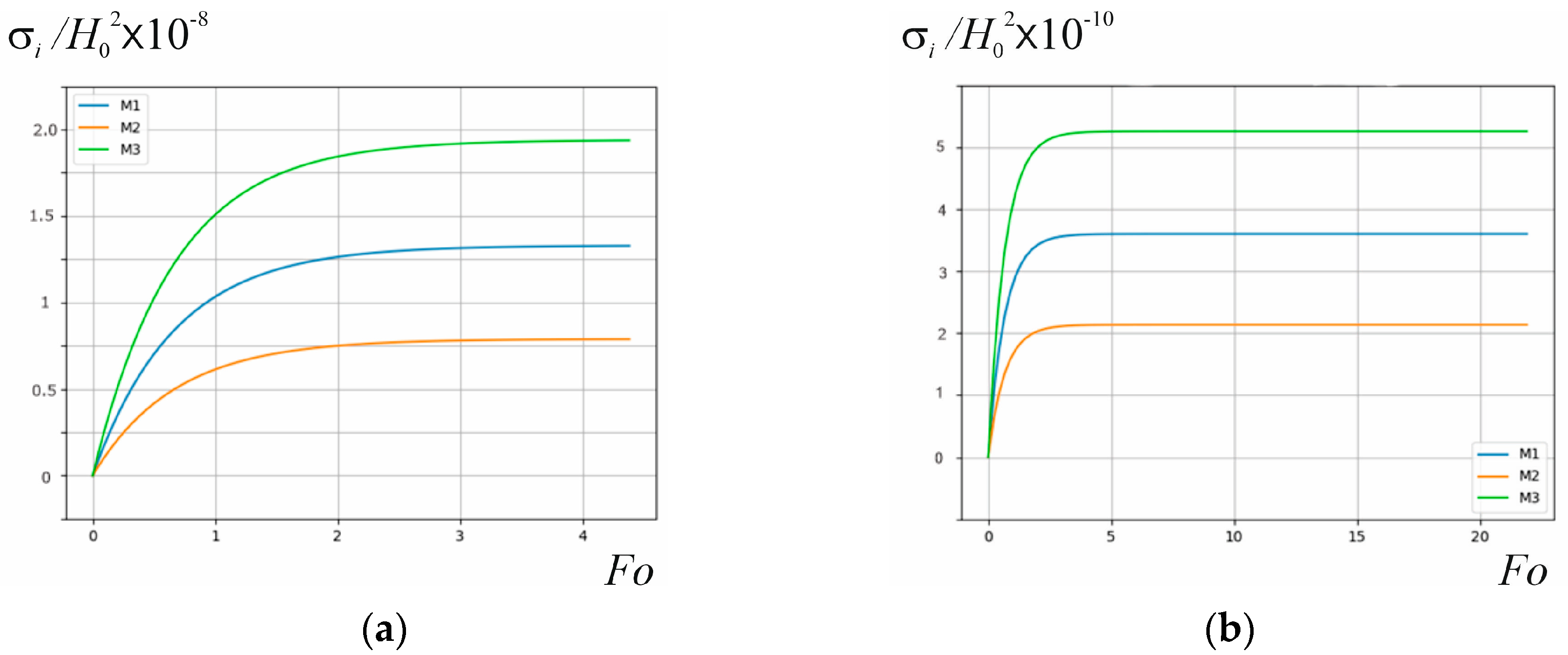
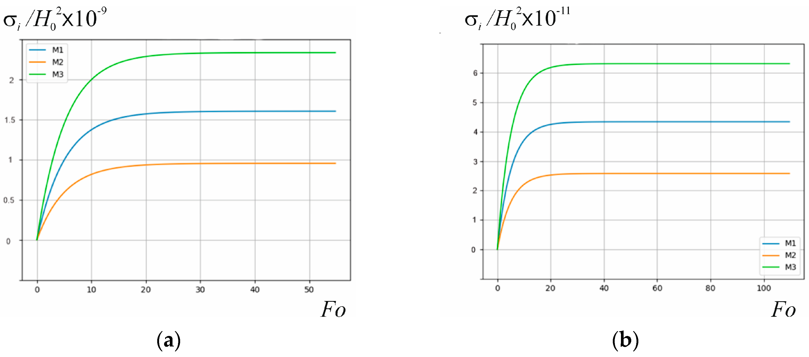
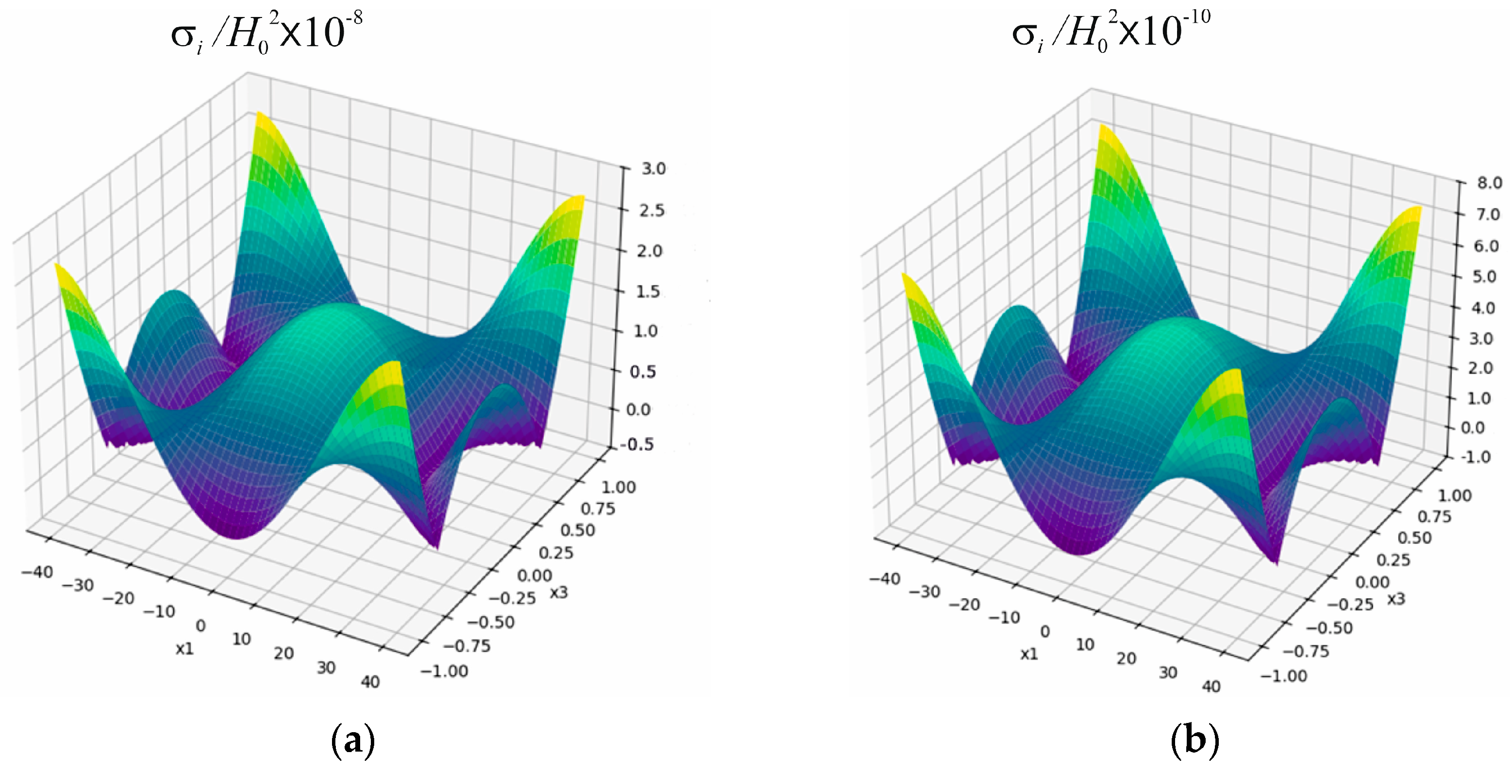
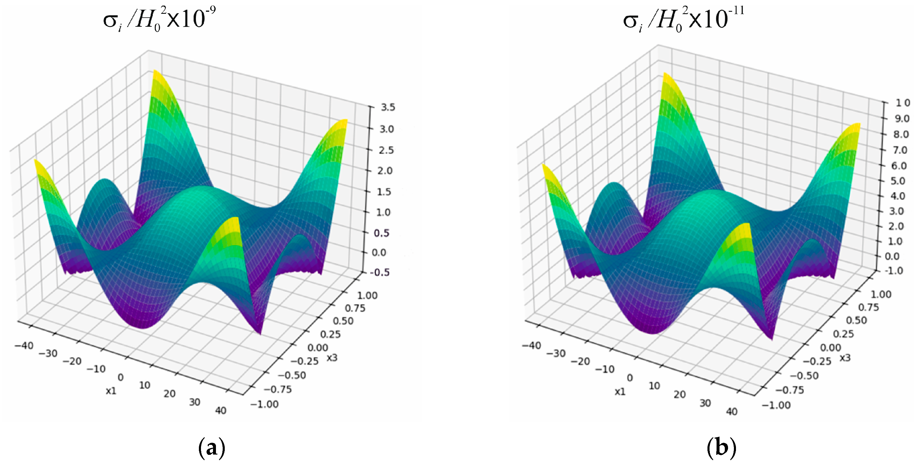
3.2. Analysis of Stress Intensity

Figure 1 shows the change in the dimensionless Fourier time Fo of the stress intensity ${\sigma }_i/H_0^2$ under near-surface at ${\delta }_0=0,1$ (Figure 1a), induction heating and continuous at ${\delta }_0=1$ (Figure 1b), and induction heating by quasi-steady-state EMF at the value of the Biot criterion $Bi=1$.

Figure 2 shows the change in the dimensionless Fourier time $Fo$ of the stress intensity ${\mathsf{\sigma }}_i/H_0^2$ during near-surface induction heating at ${\mathsf{\delta }}_0=0.1$ (Figure 2a) and continuous induction heating at ${\mathsf{\delta }}_0=1$ (Figure 2b) by quasi-steady EMF at the value of the Biot criterion $Bi=0.1$.

Figure 3 shows the variation of the stress intensity ${\sigma }_i/H_0^2$ over the cross-sectional area of the plate under consideration at the value of the Biot criterion $Bi=1$ and the Fourier time $Fo=4$ (corresponding to the time when the stress intensity reaches its maximum value) under induction heating by quasi-steady-state EMF at ${\delta }_0=0.1$ (Figure 3a) and at ${\delta }_0=1$ (Figure 3b).

Figure 4 shows the change in the stress intensity ${\sigma }_i/H_0^2$ over the cross-sectional area of the plate under consideration at the value of the Biot criterion $Bi=0.1$ and Fourier time $Fo=4$ (corresponding to the time when the stress intensity reaches its maximum value) under induction heating by a quasi-steady-state EMF at ${\delta }_0=0.1$ (Figure 4a) and at ${\delta }_0=1$ (Figure 4b).

In Figure 1, Figure 2, Figure 3 and Figure 4, the expressions of stress intensity ${\sigma }_i/H_0^2$ have the dimension $\mathrm{P}\mathrm{a}·{\mathrm{m}}^2/{\mathrm{A}}^2$.

As a result of the numerical analysis of the change in time $Fo$ of the stress intensity at the characteristic points $M_1\left(0.25d,0.25\right), M_2\left(0.5d,0.5\right), {\mathrm{and} M}_3\left(0.9d,0.9\right)$ of a rectangle of cross-section of a copper plate with half-width $d=40$ under its induction heating by a quasi-steady-state EMF, it was found that the maximum values of stress intensity in both cases—near-surface and continuous heating—occur at the point $M_3$. This means that such values of stress intensity are achieved at the corner points of the cross-sectional rectangle, i.e., on the edges of the plate. In the case of near-surface heating at ${\mathsf{\delta }}_0=0.1$, the maximum values of stress intensity are approximately 40 times higher than their maximum values for in-depth heating at ${\mathsf{\delta }}_0=1$.

It should be noted that the dependences of the stress intensity on the parameters ${\mathsf{\delta }}_0$ and $Bi$ shown in Figure 1 and Figure 2 describe the regularities of the thermomechanical behavior of the copper plate during the time $F{o}_{\ast }$ of the stress intensity reaching the steady-state mode of induction heating of the plate.

Figure 3 and Figure 4 show the distribution of the stress intensity ${\mathsf{\sigma }}_i/H_0^2$ over the cross-sectional area of the copper plate under its near-surface at ${\mathsf{\delta }}_0=0.1$ (a) and in-depth at ${\mathsf{\delta }}_0=1$ (b) induction heating for the Fourier time $Fo=F{o}_{\ast }$ of reaching the steady-state mode at which the stress intensities reach their maximum values.

The stress intensities in Figure 1, Figure 2, Figure 3 and Figure 4 are related to the value of $H_0^2$. Accordingly, their dimensional values are measured in Pascal. In the experimental studies reported in [12,15], dependencies on the density of surface currents caused by the inductor are used. When converting the current density to the magnetic field intensity, a good agreement between theoretical and experimental values was obtained.

The dependences of the maximum values of stress intensities ${\sigma }_i^{max}$ on the value of $H_0$ at different values of the parameter ${\delta }_0=0.1$ and ${\delta }_0=1$ as well as at the Biot criterion $Bi=1$ are shown in Figure 5.

Based on the above numerical analysis, we estimate the value of the stress intensity during induction heating of a copper plate in the steady-state mode. In particular, when ${Fo}_{\ast }$ = 4 ($Bi=1$, ${\delta }_0=0.1$) the real time $t_{\ast }$ to reach the steady-state mode is approximately equal to $t_{\ast }=0.03 \mathrm{s}$. Accordingly, if the heating time is $t=300 \mathrm{s}$, then at $H_0={10}^4 \mathrm{A}/\mathrm{m}$ ${\sigma }_i^{max}=20 \mathrm{k}\mathrm{P}\mathrm{a}$, and at $H_0={10}^5 \mathrm{A}/\mathrm{m}$ we have that ${\sigma }_i^{max}=2 \mathrm{M}\mathrm{P}\mathrm{a}$.

With the specified parameters of induction heat treatment at $H_0={10}^4 \mathrm{A}/\mathrm{m}$ and $H_0={10}^5 \mathrm{A}/\mathrm{m}$, the investigated copper plate retains its bearing capacity as a structural element.

4. Conclusions

On the basis of the studies performed, it was found that the maximum values of stress intensity in the copper plate under consideration during its induction heating by quasi-steady-state EMF significantly depend on the values of the dimensionless parameter ${\delta }_0$ and the Biot criterion, namely:

• the time for the stress intensity in the plate under consideration to reach the steady-state mode with a decrease in the Biot criterion by an order of magnitude in both selected cases of induction heating increases by an order of magnitude, respectively;
• at a fixed value of the parameter ${\mathsf{\delta }}_0$, with a decrease in the value of the Biot criterion, the values of stress intensity at the considered characteristic points of the plate cross-section approach the same value. In particular, at the value $Bi\le 0.01$, they are already practically the same. This is due to the fact that the nature of the plate heating regime approaches the conditions of thermal insulation of its bases and end surfaces;
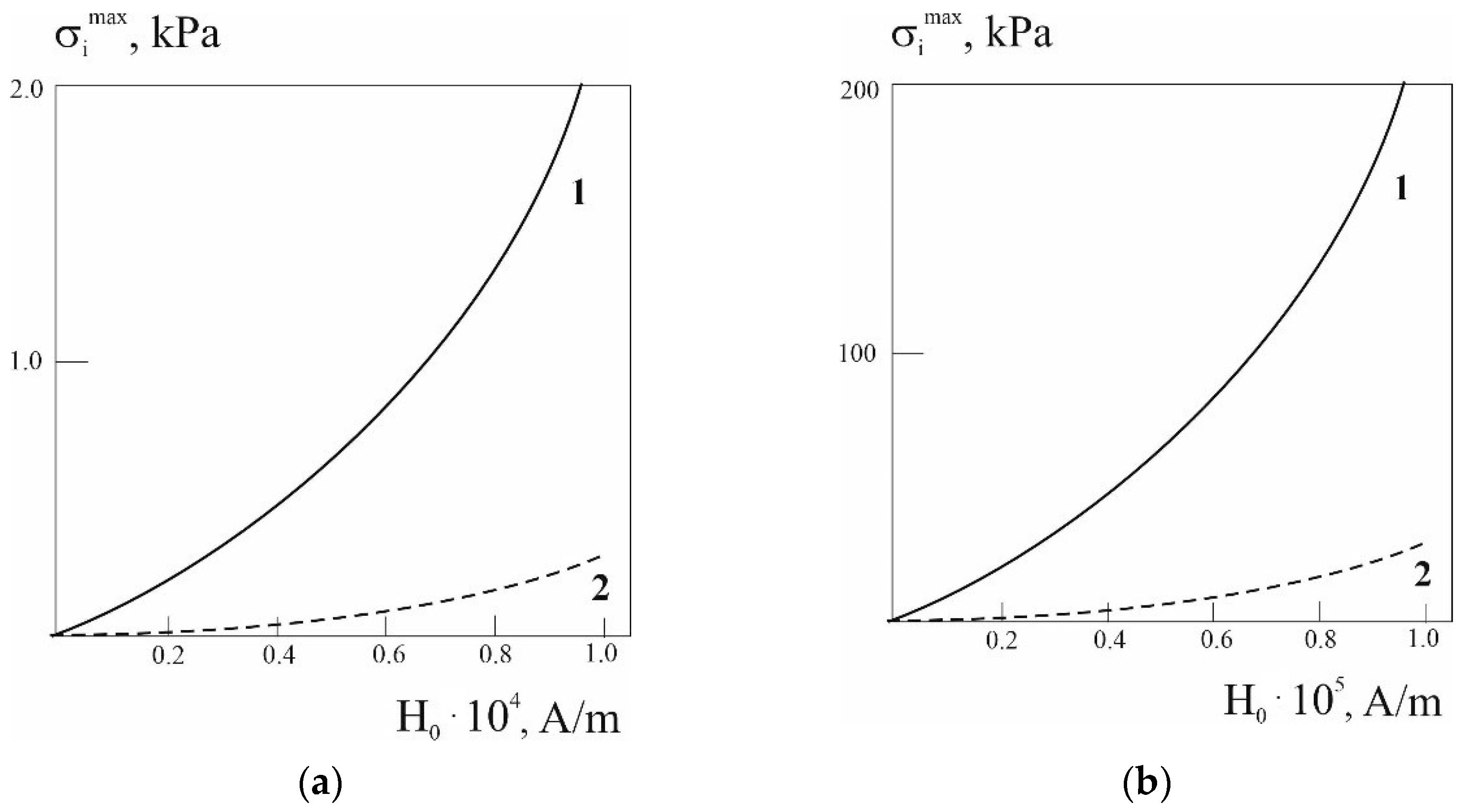
• under the conditions of near-surface heating at ${\mathsf{\delta }}_0=0.1$, the maximum values of stress intensity are approximately 40 times higher than their values under the conditions of in-depth heating at ${\mathsf{\delta }}_0=1$, regardless of the value of the Biot criterion. Thus, to achieve higher maximum values of stress intensity in a copper plate, it is advisable to use its surface heating;
• at the same value of ${\mathsf{\delta }}_0=0.1$ and ${\mathsf{\delta }}_0=1$ with a decrease in the Biot criterion by an order of magnitude, the maximum values of stress intensity decrease by approximately an order of magnitude;
• with an increase in the value of $H_0$, which corresponds to the amplitude of steady-state electromagnetic oscillations, in both cases of surface and in-depth induction heating, the maximum values of stress intensity increase according to the quadratic law.

The numerical analysis of the stress intensity in a copper plate, depending on the conditions of induction heating and convective heat exchange of the plate with the external environment, and the new qualitative and quantitative regularities revealed in this work are of important theoretical and applied significance. They are the scientific basis for engineering calculations to select the optimal parameters characterizing the induction heating of a copper plate element (parameter ${\mathsf{\delta }}_0$) and the conditions of its heat exchange with the external environment (Biot criterion). On this basis, it is possible to predict the magnitude of the stress intensity and the bearing capacity of the plate under consideration as a structural element, depending on the modes of induction heating of the plate by a quasi-steady electromagnetic field.

References

1. Lupi, S. Fundamentals of Electroheat. In Electrical Technologies for Process Heating; Springer: Cham, Switzerland, 2017. [Google Scholar] [CrossRef]
2. Lee, K.S.; Kim, S.W.; Eom, D.H. Temperature distribution and bending behaviour of thick metal strip by high frequency induction heating. Materials 2011, 15 (Suppl. S1), s283–s287. [Google Scholar]
3. Bobart, G.F. Induction Heating. AccessScience. 2020. Available online: https://www.accessscience.com/content/article/a341500 (accessed on 15 May 2023).
4. Barglik, J. Induction hardening of steel elements with complex shapes. Przegląd Elektrotech. 2018, 94, 51–54. [Google Scholar] [CrossRef]
5. Holman, J.P. Heat Transfer, 10th ed.; McGraw Hill: New York, NY, USA, 2009. [Google Scholar]
6. Hetnarski, R. Encyclopedia of Thermal Stresses; Springer: Dordrecht, The Netherlands, 2014. [Google Scholar] [CrossRef]
7. Lucía, O.; Maussion, P.; Dede, E.J.; Burdío, J.M. Induction Heating Technology and Its Applications: Past Developments, Current Technology, and Future Challenges. IEEE Trans. Ind. Electron. 2014, 61, 2509–2520. [Google Scholar] [CrossRef]
8. Drobenko, B.; Vankevych, P.; Ryzhov, Y.; Yakovlev, M. Rational approaches to high temperature induction heating. Int. J. Eng. Sci. 2017, 117, 34–50. [Google Scholar] [CrossRef]
9. Shen, H.; Yao, Z.Q.; Shi, Y.J.; Hu, J. Study on temperature field in high frequency induction heating. Acta Metall. Sin. 2006, 19, 190–196. [Google Scholar] [CrossRef]
10. Masoodi, A.R.; Arabi, E. Geometrically nonlinear thermomechanical analysis of shell-like structures. J. Therm. Stress. 2017, 41, 37–53. [Google Scholar] [CrossRef]
11. Rezaiee-Pajand, M.; Masoodi, A.R.; Arabi, E. On the shell thickness-stretching effects using seven-parameter triangular element. Eur. J. Comput. Mech. 2018, 27, 163–185. [Google Scholar] [CrossRef]
12. Grytsiuk, V.Y.; Yassin, M.A.M. Numerical modeling of coupled electromagnetic and thermal processes in the zone induction heating system for metal billets. Electr. Eng. Electromech. 2025, 59–68. [Google Scholar] [CrossRef]
13. Shcherba, A.A.; Podoltsev, O.D.; Suprunovska, N.I.; Bilianin, R.V.; Antonets, T.Y.; Masluchenko, I.M. Modeling and analysis of electro-thermal processes in installations for induction heat treatment of aluminum cores of power cables. Electr. Eng. Electromech. 2024, 1, 51–60. [Google Scholar] [CrossRef]
14. Chandrasekaran, S.; Basak, T.; Ramanathan, S. Experimental and theoretical investigation on microwave melting of metals. J. Mater. Process. Technol. 2011, 211, 482–487. [Google Scholar] [CrossRef]
15. Zhang, S.; Liu, C.; Wang, X. Temperature and deformation analysis of ship hull plate by moving induction heating using double-circuit inductor. Mar. Struct. 2019, 65, 32–52. [Google Scholar] [CrossRef]
16. Zhang, X.; Chen, C.; Liu, Y. Numerical analysis and experimental research of triangle induction heating of the rolled plate. Proc. Inst. Mech. Eng. Part C 2015, 231, 844–859. [Google Scholar] [CrossRef]
17. Fisk, M.; Ristinmaa, M.; Hultkrantz, A.; Lindgren, L.-E. Coupled electromagnetic-thermal solution strategy for induction heating of ferromagnetic materials. Appl. Math. Model. 2022, 111, 818–835. [Google Scholar] [CrossRef]
18. Naar, R.; Bay, F. Numerical optimisation for induction heat treatment processes. Appl. Math. Model. 2013, 37, 2074–2085. [Google Scholar] [CrossRef]
19. Hachkevych, O.; Musii, R. Mathematical modeling in thermomechanics of electroconductive bodies under the action of the pulsed electromagnetic fields with modulation of amplitude. Math. Model. Comput. 2019, 6, 30–36. [Google Scholar] [CrossRef]
20. Hachkevych, O.R.; Musii, R.S.; Melnyk, N.B.; Dmytruk, V.A. Dynamic thermoelastic processes in a conductive plate under the action of electromagnetic pulses of microsecond and nanosecond durations. J. Therm. Stress. 2019, 42, 1110–1122. [Google Scholar] [CrossRef]
21. Rudnev, V.; Loveless, D.; Cook, R. Handbook of Induction Heating, 2nd ed.; CRC Press: London, UK; Taylor and Francis Group: Abingdon, UK, 2018. [Google Scholar]
22. Podstryhach, Y.S.; Burak, Y.Y.; Hachkevych, A.R.; Cherniavskaia, L.V. Termoupruhost Elektroprovodnykh Tel; Nauk. Dumka: Kyiv, Ukraine, 1977. [Google Scholar]
23. Musii, R.S. Equations in stresses for the three-, two-, and one-dimensional dynamic problems of thermoelasticity. Mater. Sci. 2000, 36, 170–177. [Google Scholar] [CrossRef]
24. Musii, R.S. Constructing solutions for two-dimensional quasi-static problems of thermomechanics in terms of stresses for bodies with plane-parallel boundaries. Math. Model. Comput. 2024, 11, 995–1002. [Google Scholar] [CrossRef]
25. Musii, R.S. Thermal stressed state of a conducting plate under the action of electromagnetic pulses. Mater. Sci. 2001, 37, 845–856. [Google Scholar] [CrossRef]
26. Halytsyn, A.S.; Zhukovskyi, A.N. Yntehralnye Preobrazovanyia y Spetsyalnye Funktsyy v Zadachakh Teproprovodnosty; Nauk. Dumka: Kyiv, Ukraine, 1976. [Google Scholar]
27. Musii, R.; Lis, M.; Pukach, P.; Chaban, A.; Szafraniec, A.; Vovk, M.; Melnyk, N. Analysis of Varying Temperature Regimes in a Conductive Strip during Induction Heating under a Quasi-Steady Electromagnetic Field. Energies 2024, 17, 366. [Google Scholar] [CrossRef]
28. Timoshenko, S.; Goodier, J.N. Theory of Elasticity; McGraw—Hill: New York, NY, USA, 1970; Volume 970, pp. 279–291. [Google Scholar]
29. Thompson, M. Base Metals Handbook, 2nd ed.; Woodhead Publishing: Cambridge, UK, 2006. [Google Scholar] [CrossRef]
Figure 1. Time variation F o of the stress intensity σ i / H 0 2 in a copper plate with a thickness of 2   h = 2   m m and a width of 2 d = 80   m m at points M 1 ( 0.25 d , 0.25   h ) , M 2 ( 0.5 d , 0.5   h ) , M 3 ( 0.9 d , 0.9   h ) (lines M1–M3) at the value of the Biot criterion B i = 1 during its induction heating: (a) δ 0 = 0.1 ; (b) δ 0 = 1 .
Symmetry 17 00754 g001
Figure 2. Time variation F o of the stress intensity σ i / H 0 2 in a copper plate with a thickness of 2   h = 2   m m and a width of 2 d = 80   m m at points M 1 ( 0.25 d , 0.25   h ) , M 2 ( 0.5 d , 0.5   h ) , and   M 3 ( 0.9 d , 0.9   h ) (lines M1–M3) at the value of the Biot criterion B i = 0.1 during its induction heating: (a) δ 0 = 0.1 ; (b) δ 0 = 1 .
Symmetry 17 00754 g002
Figure 3. Variation of the stress intensity σ i / H 0 2 over the cross-sectional area of an copper plate with a thickness of 2   h = 2   m m and a width of 2 d = 80   m m at the value of the Biot criterion B i = 1 and the Fourier time F o = 4 under its surface at induction heating: (a) δ 0 = 0.1 ; (b) δ 0 = 1 .
Symmetry 17 00754 g003
Figure 4. Variation of the stress intensity σ i / H 0 2 over the cross-sectional area of a copper plate with a thickness of 2   h = 2   m m and a width of 2 d = 80   m m at the value of the Biot criterion B i = 0.1 and the Fourier time F o = 4 under its surface at induction heating: (a) δ 0 = 0.1 ; (b) δ 0 = 1 .
Symmetry 17 00754 g004
Figure 5. Dependence of the maximum values of stress intensities σ i m a x the value of H 0 at different values of the parameter δ 0 : (a) H 0 = 10 4   A / m ; (b) H 0 = 10 5   A / m . Lines 1 correspond to the value of the parameter δ 0 = 0.1 , and lines 2 correspond to the value of the parameter δ 0 = 1 .
Symmetry 17 00754 g005
Disclaimer/Publisher’s Note: The statements, opinions and data contained in all publications are solely those of the individual author(s) and contributor(s) and not of MDPI and/or the editor(s). MDPI and/or the editor(s) disclaim responsibility for any injury to people or property resulting from any ideas, methods, instructions or products referred to in the content.