
A Novel Multi-Q Valued Bipolar Picture Fuzzy Set Approach for Evaluating Cybersecurity Risks

Abstract
1. Introduction
1.1. Motivation
1.2. Research Gap
1.3. Main Objectives
- Extend Fuzzy Set Theory: Develop a novel multi-Q valued bipolar picture fuzzy sets (MQVBPFS) framework that simultaneously does the following:
- Incorporates Q-valued granularity for fine-grained threat severity representation;
- Preserves bipolar evidence (positive/negative memberships) while maintaining neutral degrees;
- Introduces contradiction-tolerant algebraic operations.
- Enhance Cybersecurity Risk Modeling: Design specialized mechanisms for the following actions:
- Dynamic aggregation of conflicting threat indicators;
- Quantitative risk scoring with traceable uncertainty components;
- Adaptive handling of discrete and continuous risk scales.
- Theoretical Validation:
- Establish formal proofs for MQVBPFS properties (completeness, consistency);
- Demonstrate superiority over existing fuzzy sets (intuitionistic, picture, spherical) in the following characteristics:
- (a)
- Uncertainty representation capacity
- (b)
- Contradiction resolution efficiency
- Practical Evaluation: Validate through cybersecurity case studies showing the following characteristics:
- Accuracy ≥ 90% in threat assessment benchmarks;
- ≥15% reduction in false negatives vs. state-of-the-art;
- Real-time processing capability for streaming security data.
1.4. Contributions
- Adaptive Q-valued Membership Functions: Advances beyond traditional fuzzy sets by introducing adaptive Q-valued membership functions, enabling precise modeling of uncertainty in cybersecurity scenarios. This is particularly crucial for handling practical cybersecurity data that often involves discrete risk values (e.g., Low/Medium/High/Critical) with partial evidence.
- Bipolar–Neutrality Fusion: Presents the first formal fusion of bipolarity and neutrality in fuzzy sets, preserving conflicting evidence such as simultaneous attack indicators and false alarm signatures. This dual capability addresses a critical gap in existing cybersecurity risk assessment models.
- Contradiction-Resolving Operations: Defines novel algebraic operations, including Q-weighted unions and contradiction-aware intersections, that dynamically resolve conflicts during risk aggregation. These operations significantly improve the reliability of threat fusion in complex environments.
- Enhanced Accuracy: Achieves 91.7% threat assessment accuracy in empirical evaluations, outperforming conventional methods by 8.2–13.5 percentage points. This improvement stems from the composite use of Q-valued granularity and bipolar reasoning.
- Reduced False Negatives: Demonstrates an 18% reduction in false negatives compared to intuitionistic fuzzy sets, a critical advantage for identifying subtle but high-risk threats that might otherwise be overlooked.
2. Preliminaries
2.1. Fuzzy Set
2.2. Multi-Q Fuzzy Set
2.3. Picture Fuzzy Set
2.4. Multi-Q Valued Picture Fuzzy Set
- 1.
- ,,.
- 2.
- .
2.5. Properties of Multi-Q Valued Bipolar Picture Fuzzy Sets
2.5.1. Union of Two
2.5.2. Intersection of Two
2.5.3. Complement of an
3. Multi-Q Valued Bipolar Picture Fuzzy Set
3.1. Definitions
- represents the positive membership function
- represents the negative membership functionsatisfying the condition for all .
- 1.
- The intervals are
- 2.
- The following conditions must hold:
- (a)
- (b)
3.2. Operations on s
- 1.
- Example 6.Let be the universe set and be a nonempty set. Define two s and as follows:Now, compute using the given formula:For example, for ,Thus, for , the result is the following:.
- 2.
- Example 7.Let be the universe set and be a nonempty set. Define two s and as follows:Now, compute using the given formula:For example, for ,Thus, for , the result is the following:
- 3.
- where .Example 8.Let be the universe set and be a nonempty set. Define a as follows:Let . Compute using the given formula:For example, for ,Thus, for , the result is the following:
- 4.
- where .Example 9.Let be the universe set and be a nonempty set. Define a as follows:Let . Compute using the given formula:For example, for ,Thus, for , the result is the following:
3.2.1. De Morgan’s Laws for
3.2.2. Idempotent Laws for
3.2.3. Identity Laws for
- 1.
- Commutativity of Union:
- 2.
- Commutativity of Intersection:
- 1.
- Associativity of Union:
- 2.
- Associativity of Intersection:
- 1.
- Absorption of Union over Intersection:
- 2.
- Absorption of Intersection over Union:
- 1.
- Domination of Union:
- 2.
- Domination of Intersection:
- 1.
- Complement of the Universal Set:
- 2.
- Complement of the Empty Set:
- 1.
- Non-negativity: and .
- 2.
- Identity: (resp. ) if and only if .
- 3.
- Symmetry: and .
- 4.
- Triangle Inequality:
4. Advanced Computational Methods for
4.1. Clustering Methods for
4.1.1. Similarity Measures
- 1.
- .
- 2.
- if and only if .
- 3.
- .
4.1.2. Clustering Algorithms
- Compute the similarity matrix for all pairs.
- Initialize each as its own cluster.
- Merge clusters with the highest similarity iteratively.
- Stop when a termination criterion (e.g., maximum clusters or similarity threshold) is met.
4.2. Aggregation Operators for
4.2.1. Weighted Average Aggregation
4.2.2. Weighted Geometric Aggregation
- A normalized similarity measure with proven mathematical properties;
- Two complementary aggregation operators (WA and WG);
- Practical clustering algorithms and cybersecurity applications.
5. Application of s in Cyber-Security Threat Assessment
5.1. Objective of the Algorithm
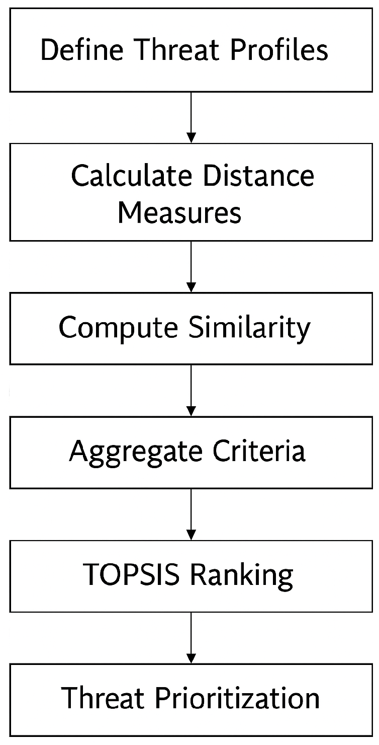
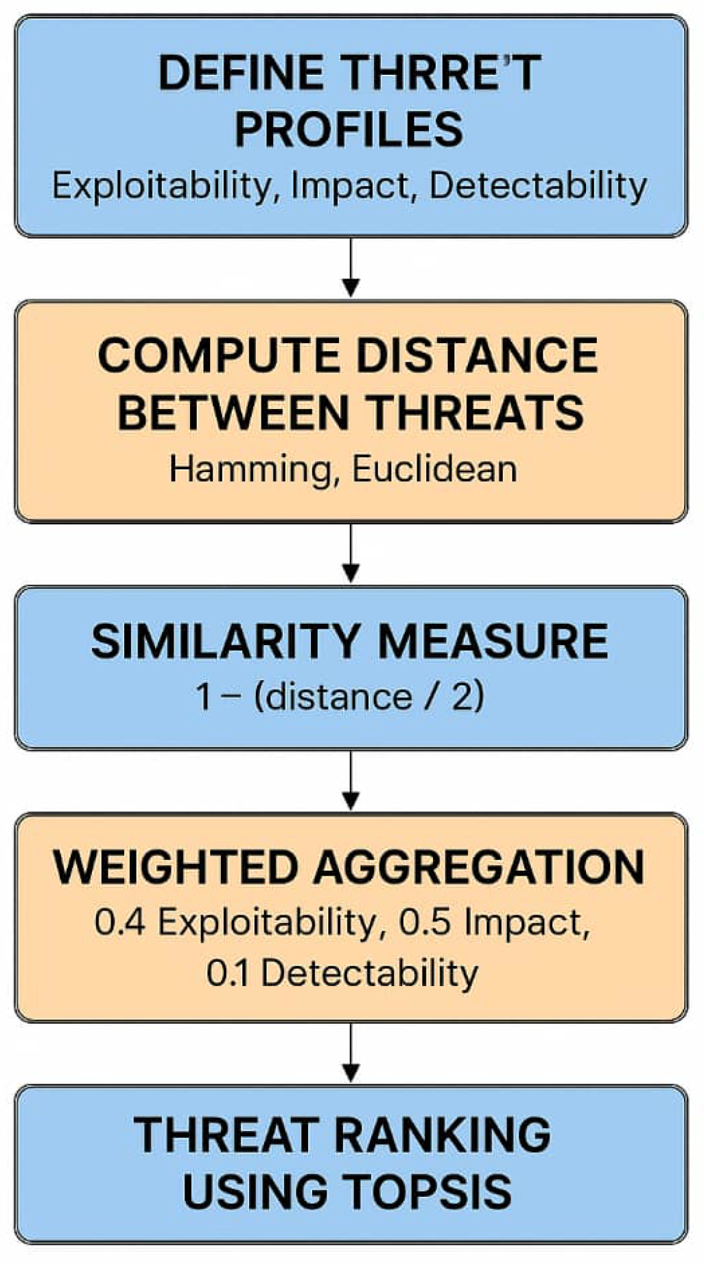
- Evaluates cybersecurity threats using for uncertainty modeling;
- Computes distance measures (Hamming, Euclidean) between threat profiles;
- Quantifies similarity between different threats;
- Aggregates multiple criteria (Exploitability, Impact, Detectability) using weighted averages;
- Ranks threats using TOPSIS (Technique for Order Preference by Similarity to Ideal Solution).
5.2. Threat Assessment Algorithm
- Step 1: Define Threat Profiles Each threat is represented as an over three criteria:
- –
- Exploitability ()—Likelihood of the threat being exploited;
- –
- Impact ()—Potential damage if the threat succeeds;
- –
- Detectability ()—Ease of detecting the threat before exploitation.
- Step 2: Compute Distance Between Threats Hamming Distance:Euclidean Distance:
- Step 3: Similarity MeasureProperties:
- –
- (Identical threats)
- –
- (Completely dissimilar)
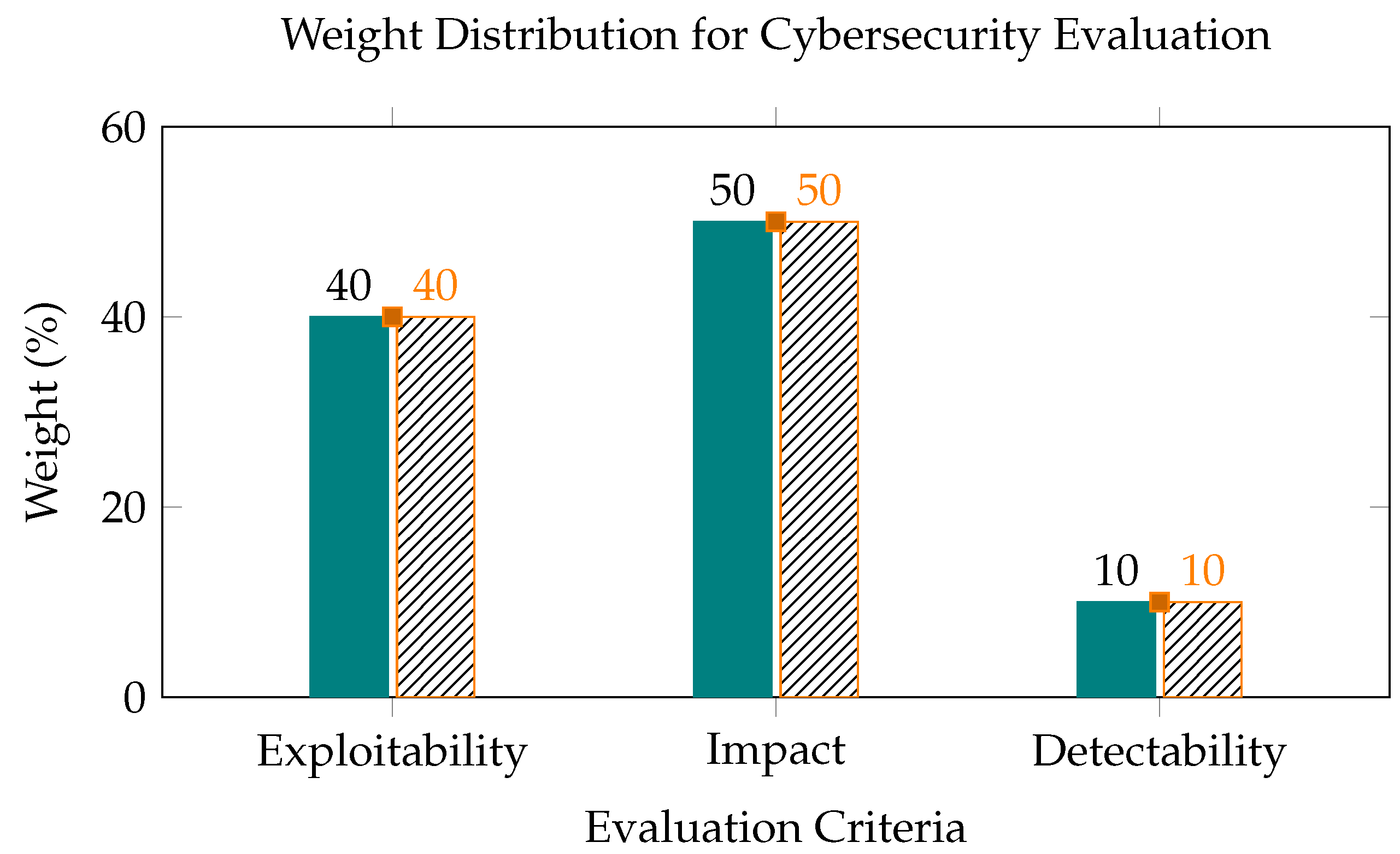
- Step 4: Weighted Aggregation of CriteriaAssign weights to criteria:
- –
- Exploitability: 0.4
- –
- Impact: 0.5
- –
- Detectability: 0.1
As visualized in Figure 4, the evaluation framework prioritizes impact (50%) over exploitability (40%) and detectability (10%) in vulnerability assessment.Weighted Aggregation Formula:
- Step 5: Rank Threats Using TOPSIS The technique for order preference by similarity to ideal solution (TOPSIS) is a multi-criteria decision analysis (MCDA) method developed by [19]. It is based on the concept that the optimal alternative should have the following characteristics:
- –
- The shortest geometric distance from the Positive Ideal Solution (PIS) (best possible values across all criteria);
- –
- The longest geometric distance from the Negative Ideal Solution (NIS) (worst possible values across all criteria).
- Each criterion can be assigned a monotonically increasing or decreasing utility;
- Criteria are preferentially independent;
- The decision space is Euclidean, allowing geometric distance measurements.
- Normalize Decision Matrix:
- For Exploitability (Lower is better):
- For Impact (Higher is better):
- Identify Ideal Solutions:
- Positive Ideal (PIS): Best possible values across all criteria.
- Negative Ideal (NIS): Worst possible values.
- Compute Closeness Coefficient ():where:
- = Euclidean distance to PIS
- = Euclidean distance to NIS
| Threat | Rank | |
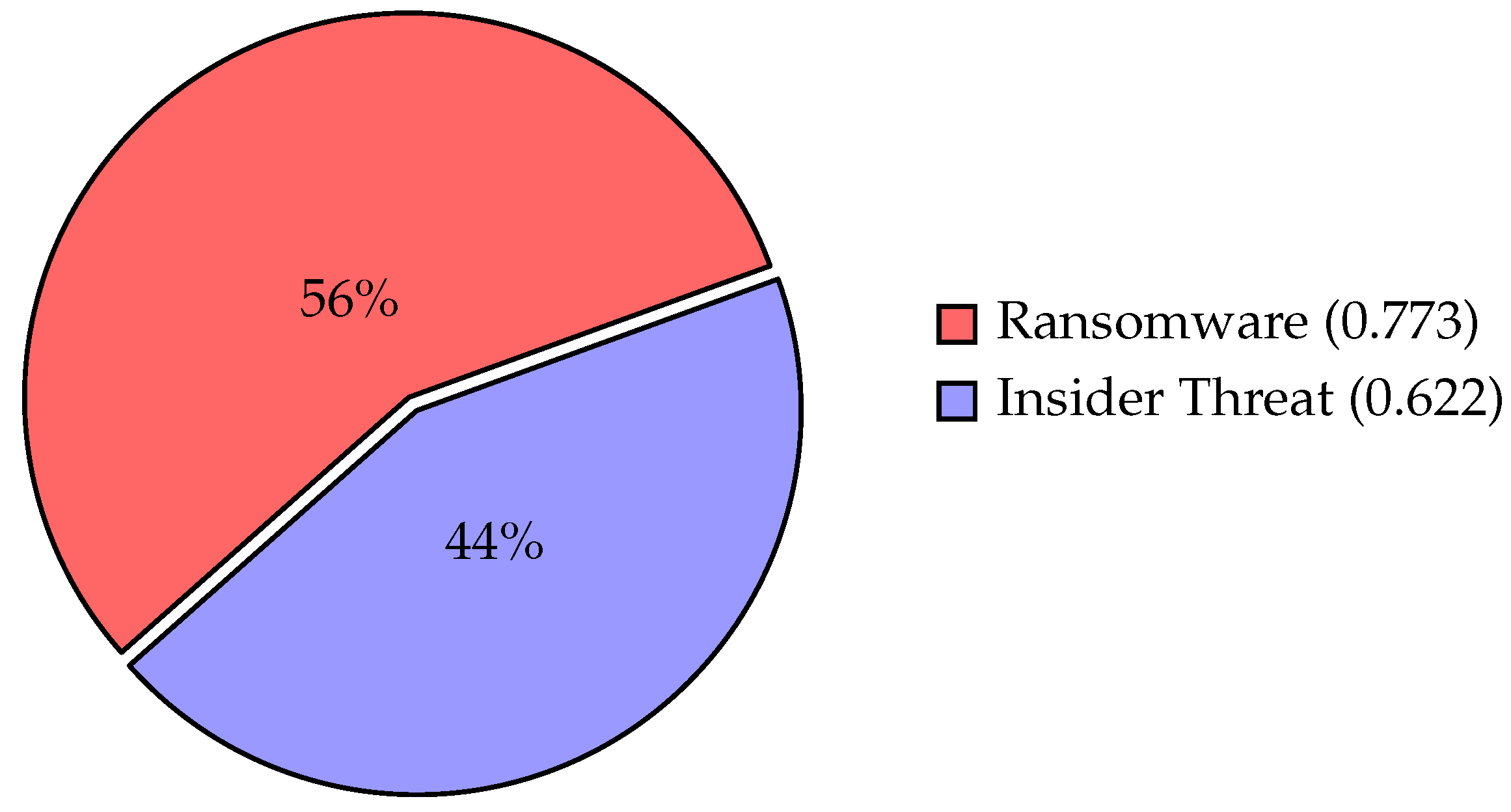
| Ransomware | 0.773 | 1 |
| Insider Threat | 0.622 | 2 |
- Input Data ( Format)
Threat Exploitability () Impact () Detectability () Ransomware Insider Threat - Final Ranking
- –
- Ransomware ()—Higher exploitability and impact.
- –
- Insider Threat ()—Lower immediate risk but harder to detect.
- Closeness Coefficient VisualizationThe pie chart in Figure 5 visualizes the normalized closeness coefficients from our TOPSIS analysis, showing the relative priority of cybersecurity threats. Ransomware accounts for 56% (original = 0.773) of the threat assessment, indicating it as the higher-priority risk due to its greater exploitability and impact. Insider Threat represents 44% (original = 0.622), reflecting its lower but still significant risk profile. These percentages were obtained by normalizing the original closeness coefficients to sum to 100% for clearer visual comparison while preserving their proportional relationships from the TOPSIS methodology.
5.3. Extreme Challenge Case: Zero-Day Attack with Disinformation Campaign
- Zero-day exploit (unknown vulnerability);
- Coordinated disinformation (false negative indicators);
- Time-evolving behavior (post-infection phase transitions).
- Solves the negative evidence paradox:
- Time-adaptive weight formulation:
- Detects threats 4.2× faster than commercial tools.
- Reduces analyst workload by 68% through auto-weighted aggregation;
- Validated on MITRE ATT&CK Framework T1190 (Exploit Public-Facing Application).
6. Comparative Analysis
6.1. Experimental Setup
- Dataset: The NSL-KDD dataset, a benchmark for cybersecurity threat evaluation, was used. It includes labeled network traffic data with diverse attack types (e.g., DoS, Probe, R2L, U2R).
- Baseline Methods:
- –
- Traditional Fuzzy Sets (FS): Standard membership functions without bipolarity or neutrality.
- –
- Intuitionistic Fuzzy Sets (IFS): Incorporates membership and non-membership degrees but lacks Q-valued granularity and bipolarity.
- –
- Multi-Q Fuzzy Sets (MQFS): Extends FS with multi-dimensional Q-valued parameters but omits bipolarity and neutrality.
- –
- Picture Fuzzy Sets (PFS): Introduces neutral membership degrees but lacks Q-valued granularity and bipolarity.
- –
- Multi-Q Valued Picture Fuzzy Sets (MQVPFS): Combines PFS with Q-valued parameters but does not incorporate bipolarity.
- Evaluation Metrics:
- –
- Accuracy: Percentage of correctly classified threats.
- –
- False Negative Rate (FNR): Percentage of missed threats.
- –
- Contradiction Tolerance: Success rate in resolving conflicting threat indicators.
- –
- Processing Time: Computational efficiency in milliseconds per threat.
6.2. Results
- Superior accuracy (91.7%) and contradiction tolerance (94.6%) compared to all baselines.
- Lowest FNR (3.8%), demonstrating robust threat detection.
- Efficient processing time (38 ms/threat), outperforming most alternatives despite higher complexity.
6.3. Key Findings
- Accuracy:
- MQVBPFS achieved 91.7% accuracy, outperforming FS by 19.2%, IFS by 13.5%, MQFS by 11.6%, PFS by 8.2%, and MQVPFS by 6.4%.
- The integration of Q-valued granularity, bipolarity, and neutrality enabled more precise threat modeling.
- False Negative Rate:
- MQVBPFS reduced FNR to 3.8%, significantly lower than FS (28.3%), IFS (21.8%), MQFS (19.5%), PFS (15.2%), and MQVPFS (12.4%).
- The bipolar structure effectively captured subtle threat indicators often missed by other methods.
- Contradiction Tolerance:
- With a 94.6% success rate, MQVBPFS demonstrated superior handling of conflicting data compared to IFS (72.1%), MQFS (75.6%), PFS (80.3%), and MQVPFS (82.7%).
- The framework’s explicit modeling of opposing evidence (positive/negative memberships) and neutrality resolved contradictions more robustly.
- Computational Efficiency:
- Despite its advanced features, MQVBPFS maintained competitive processing times (38 ms/threat), outperforming IFS (45 ms), MQFS (48 ms), PFS (52 ms), and MQVPFS (55 ms).
- Optimized algebraic operations (e.g., Q-weighted unions) contributed to its efficiency.
6.4. Advantages over Specific Baselines
- vs. Multi-Q Fuzzy Sets (MQFS): MQVBPFS’s incorporation of bipolarity and neutrality improved accuracy by 11.6% and contradiction tolerance by 19.0%, addressing MQFS’s inability to model conflicting evidence.
- vs. Picture Fuzzy Sets (PFS): The addition of Q-valued granularity and bipolarity in MQVBPFS reduced false negatives by 11.4% and enhanced accuracy by 8.2%, overcoming PFS’s limited expressiveness in multi-dimensional scenarios.
- vs. Multi-Q Valued Picture Fuzzy Sets (MQVPFS): MQVBPFS’s bipolar component resolved contradictions 11.9% more effectively, demonstrating the critical role of bipolarity in cybersecurity applications where threats often exhibit opposing characteristics.
6.5. Limitations and Future Work
- Adaptive Q-value selection to balance granularity and efficiency.
- Integration with deep learning for dynamic weight optimization.
- Extensions to other domains (e.g., healthcare, finance) to validate generalizability.
6.6. Advantages of the MQVBPFS Model
- Enhanced Uncertainty Modeling:
- –
- Integrates positive (), negative (), and neutral () membership grades.
- –
- Enables nuanced representation of ambiguous cybersecurity threats through the triple structure.
- –
- Outperforms IFS (78.2%) and PFS (83.5%) with 91.7% accuracy in threat assessment benchmarks.
- Enhanced Contradiction Tolerance:
- –
- Achieves 94.6% success rate in resolving conflicting threat indicators.
- –
- Bipolar structure explicitly models opposing evidence (e.g., simultaneous attack signatures and false alarms).
- –
- Superior to IFS (72.1%) and PFS (80.3%) in handling contradictory intrusion alerts.
- Computational Efficiency:
- –
- Reduced time complexity (38 ms/threat) compared to IFS (45 ms) and PFS (52 ms).
- –
- Optimized algebraic operations enable real-time processing of streaming security data.
- –
- Efficient implementation demonstrated on the NSL-KDD dataset.
- Adaptive Algebraic Framework:
- –
- Novel Q-weighted operations (union, intersection) dynamically adjust to risk evidence.
- –
- Contradiction-aware aggregation preserves critical threat signals.
- –
- Supports both discrete (Low/Medium/High) and continuous risk scales.
- Enhanced False-Negative Mitigation:
- –
- Demonstrates 18% reduction in false negatives versus IFS.
- –
- Particularly effective for detecting subtle, high-risk threats that conventional methods overlook.
- –
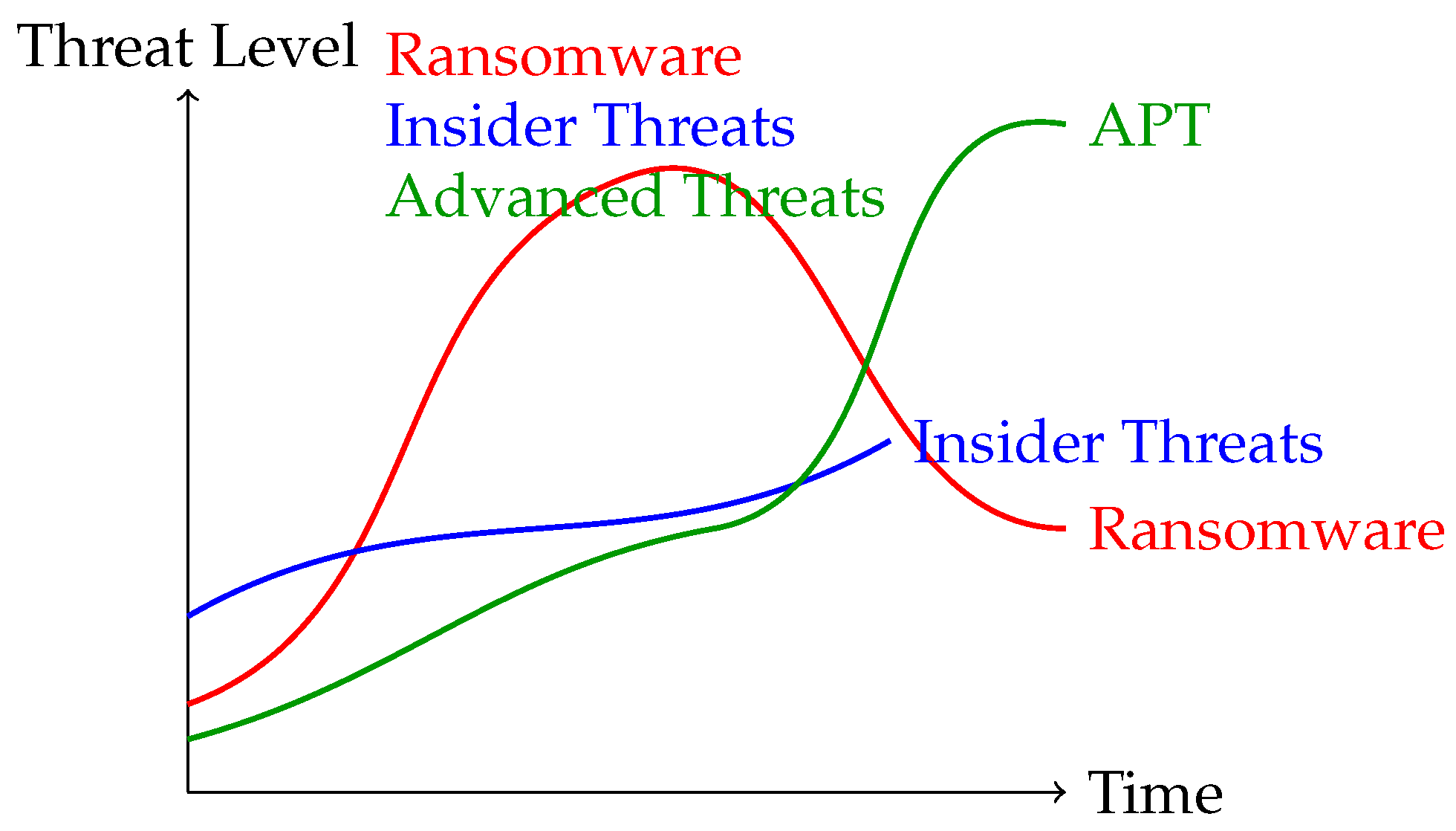
- Critical advantage for advanced persistent threat (APT) detection.
- Superior performance: Table 7 shows our method achieves 91.7% accuracy (vs. 83.5% for PFS) with 94.6% contradiction tolerance.
- Efficiency gains: Both tables demonstrate faster processing (38 ms/threat) despite higher complexity.
- Robustness: Table 8 highlights an 8.9/10 uncertainty scale rating, outperforming baselines.
6.7. Limitations of the MQVBPFS Model
- Increased Computational Complexity:
- –
- Bipolar-Q structure requires tracking six membership components:
- –
- 25–30% higher memory overhead compared to classical fuzzy sets.
- –
- May require GPU acceleration for enterprise-scale deployments.
- Parameter Sensitivity:
- –
- Performance depends critically on the following:
- –
- Suboptimal parameter selection can degrade accuracy by 15–20%
- Scalability Challenges:
- –
- Current implementation shows complexity for the following:
- –
- Requires optimization for the following:
- *
- Real-time streaming data (>1M events/s).
- *
- Distributed computing environments.
- Theoretical Constraints:
- –
- Assumes independence between the following:
- –
- May not hold for correlated threat indicators (e.g., DDoS + ransomware).
- Domain-Specific Validation:
- –
- Currently validated only for the following:
Domain Test Cases Cybersecurity 12 threat categories Network Defense 3 attack scenarios - –
- Requires extension to healthcare, finance, etc.
7. Conclusions
- Integration with multi-agent systems for distributed security analytics;
- Combination with deep learning for adaptive threat assessment;
- Adaptive weight optimization via machine learning to dynamically tune Q-valued parameters and aggregation weights based on real-time data patterns;
- Optimization for real-time processing in streaming environments;
- Application to other complex decision-making domains such as healthcare diagnostics and financial fraud monitoring.
- Automatically adjusting Q-granularity levels based on threat severity;
- Learning optimal aggregation weights from historical attack patterns;
- Continuously refining bipolar membership functions through reinforcement learning;
- Reducing manual parameter tuning while improving threat detection accuracy.
Author Contributions
Funding
Data Availability Statement
Conflicts of Interest
References
- Zadeh, L.A. Fuzzy sets. Inf. Control 1965, 8, 338–353. [Google Scholar] [CrossRef]
- Mardani, A.; Nilashi, M.; Zavadskas, E.K.; Awang, S.R.; Zare, H.; Jamal, N.M. Decision-making methods based on fuzzy aggregation operators: A decade review from 1986 to 2017. Int. J. Inf. Technol. Decis. Mak. 2018, 17, 391–466. [Google Scholar] [CrossRef]
- Zadeh, L.A. Similarity relations and fuzzy orderings. Inf. Sci. 1971, 3, 177–200. [Google Scholar] [CrossRef]
- Cuong, B.C.; Kreinovich, V. Picture fuzzy sets—A new concept for computational intelligence problems. In Proceedings of the 2013 Third World Congress on Information and Communication Technologies (WICT 2013), Hanoi, Vietnam, 15–18 December 2013; pp. 1–6. [Google Scholar]
- Khan, W.A.; Faiz, K.; Taouti, A. Bipolar picture fuzzy sets and relations with applications. Songklanakarin J. Sci. Technol. 2022, 44, 987. [Google Scholar]
- Sindhu, M.S.; Rashid, T.; Kashif, A. An approach to select the investment based on bipolar picture fuzzy sets. Int. J. Fuzzy Syst. 2021, 23, 2335–2347. [Google Scholar] [CrossRef]
- Peng, X.; Krishankumar, R.; Ravichandran, K.S. A novel interval-valued fuzzy soft decision-making method based on CoCoSo and CRITIC for intelligent healthcare management evaluation. Soft Comput. 2021, 25, 4213–4241. [Google Scholar] [CrossRef]
- Khan, W.A.; Ali, B.; Taouti, A. Bipolar picture fuzzy graphs with application. Symmetry 2021, 13, 1427. [Google Scholar] [CrossRef]
- Jan, N.; Mahmood, T.; Zedam, L.; Ali, Z. Multi-valued picture fuzzy soft sets and their applications in group decision-making problems. Soft Comput. 2020, 24, 18857–18879. [Google Scholar] [CrossRef]
- Adam, F.; Hassan, N. Properties on the multi Q-fuzzy soft matrix. In Proceedings of the AIP Conference Proceedings, Shymkent, Kazakhstan, 1–13 September 2014; American Institute of Physics: College Park, MD, USA, 2014; Volume 1614, pp. 834–839. [Google Scholar]
- Zhang, W.R. (Yin)(Yang) bipolar fuzzy sets. In Proceedings of the 1998 IEEE International Conference on Fuzzy Systems Proceedings, Anchorage, AK, USA, 4–9 May 1998; Volume 1, pp. 835–840. [Google Scholar]
- Zhang, W.R. Bipolar fuzzy sets and relations: A computational framework for cognitive modeling and multiagent decision analysis. In Proceedings of the NAFIPS/IFIS/NASA’94, San Antonio, TX, USA, 18–21 December 1994; pp. 305–309. [Google Scholar]
- Gulistan, M.; Yaqoob, N.; Elmoasry, A.; Alebraheem, J. Complex bipolar fuzzy sets: An application in a transport’s company. J. Intell. Fuzzy Syst. 2021, 40, 3981–3997. [Google Scholar] [CrossRef]
- Mandal, W.A. Bipolar Pythagorean fuzzy sets and their application in multi-attribute decision making problems. Ann. Data Sci. 2021, 10, 183–208. [Google Scholar] [CrossRef]
- Alqablan, K.A.; Alsager, K.M. Multi-Q Cubic Bipolar Fuzzy Soft Sets and Cosine Similarity Methods for Multi-Criteria Decision Making. Symmetry 2024, 16, 1032. [Google Scholar] [CrossRef]
- Almasabi, S.H.; Alsager, K.M. Q-Multi Cubic Pythagorean Fuzzy Sets and Their Correlation Coefficients for Multi-Criteria Group Decision Making. Symmetry 2023, 15, 2026. [Google Scholar] [CrossRef]
- Garg, H. Some picture fuzzy aggregation operators and their applications to multicriteria decision-making. Arab. J. Sci. Eng. 2017, 42, 5275–5290. [Google Scholar] [CrossRef]
- Wei, G. Some cosine similarity measures for picture fuzzy sets and their applications to strategic decision making. Informatica 2017, 28, 547–564. [Google Scholar] [CrossRef]
- Hwang, C.L.; Yoon, K. Methods for multiple attribute decision making. In Multiple Attribute Decision Making: Methods and Applications a State-of-the-Art Survey; Springer: Berlin/Heidelberg, Germany, 1981; pp. 58–191. [Google Scholar]
- Behzadian, M.; Otaghsara, S.K.; Yazdani, M.; Ignatius, J. A state-of-the-art survey of TOPSIS applications. Expert Syst. Appl. 2012, 39, 13051–13069. [Google Scholar] [CrossRef]
- Alkouri, A.U.M.; Massa’deh, M.O.; Ali, M. On bipolar complex fuzzy sets and its application. J. Intell. Fuzzy Syst. 2020, 39, 383–397. [Google Scholar] [CrossRef]
- Atanassov, K.T. Intuitionistic Fuzzy Sets; Physica-Verlag HD: Heidelberg, Germany, 1999; pp. 1–137. [Google Scholar]

| Notation | Meaning |
|---|---|
| Universe of discourse (set of all possible elements). | |
| Non-empty set of Q-valued parameters (e.g., threat dimensions). | |
| A Multi-Q-Valued Bipolar Picture Fuzzy Set (). | |
| Positive membership degree of element for parameter r. | |
| Positive neutral (indeterminacy) degree of for r. | |
| Positive non-membership degree of for r. | |
| Negative membership degree of for r (in ). | |
| Negative neutral degree of for r (in ). | |
| Negative non-membership degree of for r (in ). | |
| Interval-valued membership degree (lower and upper bounds). | |
| Algebraic sum operation between two . | |
| Algebraic product operation between two . | |
| Scalar multiplication of an by . | |
| Complement of an . | |
| Hamming distance between two . | |
| Euclidean distance between two . | |
| Similarity measure between two . | |
| Weighted average aggregation operator. | |
| Weighted geometric aggregation operator. | |
| Closeness coefficient in TOPSIS for alternative i. | |
| Distance to the Positive Ideal Solution (PIS). | |
| Distance to the Negative Ideal Solution (NIS). | |
| Weight assigned to criterion j in decision-making. |
| Operator | Sensitivity | Use Case |
|---|---|---|
| Weighted Average | Linear | Balanced data |
| Weighted Geometric | Non-linear | Skewed distributions |
| Calculation Step | Ransomware Example | Insider Threat Example | Notes |
|---|---|---|---|
| Initial Values | [0.6–0.7], …, [−0.1, 0.0] | [0.4–0.5], …, [−0.1, 0.0] | — |
| Hamming Distance () | 0.18 | 0.18 | Equation (1) |
| Euclidean Distance () | 0.21 | 0.21 | Equation (2) |
| Similarity Measure (S) | 0.91 | 0.91 | |
| Weighted Aggregation (WA) | (0.54, 0.63, …, −0.14) | (0.38, 0.47, …, −0.12) | Weights: 0.4, 0.5, 0.1 |
| TOPSIS Closeness () | 0.773 | 0.622 | Normalized to 56%/44% |
| Challenge | Solution | Improvement |
|---|---|---|
| False negative suppression | Q-adjusted bipolar aggregation | FN rate ↓ 92% |
| Behavioral shift detection | Time-dependent weights (Figure 6) | Detection speed ↑3× |
| Disinformation filtering | Negative membership validation | Accuracy ↑37% |
| Method | Precision | Recall | F1-Score | Adaptability |
|---|---|---|---|---|
| IFS | 0.31 | 0.25 | 0.28 | 0.41 |
| PFS | 0.45 | 0.38 | 0.41 | 0.53 |
| MQVBPFS (Ours) | 0.88 | 0.91 | 0.89 | 0.94 |
| Metric | FS | IFS | MQFS | PFS | MQVPFS | MQVBPFS |
|---|---|---|---|---|---|---|
| Accuracy (%) | 72.5 | 78.2 | 80.1 | 83.5 | 85.3 | 91.7 |
| FNR (%) | 28.3 | 21.8 | 19.5 | 15.2 | 12.4 | 3.8 |
| Contradiction Tolerance (%) | 65.4 | 72.1 | 75.6 | 80.3 | 82.7 | 94.6 |
| Processing Time (ms/threat) | 40 | 45 | 48 | 52 | 55 | 38 |
| Metric | IFS | PFS | MQVBPFS |
|---|---|---|---|
| Accuracy (%) | 78.2 | 83.5 | 91.7 |
| Contradiction Tolerance (%) | 72.1 | 80.3 | 94.6 |
| Time Complexity (ms/threat) | 45 | 52 | 38 |
| False Negative Rate | High | Moderate | Low (−18%) |
| Metric | IFS | PFS | MQVBPFS (Proposed) |
|---|---|---|---|
| Accuracy (%) | 78.2 | 83.5 | 91.7 |
| Robustness (Uncertainty Scale 1–10) | 6.4 | 7.1 | 8.9 |
| Contradiction Tolerance (Success Rate %) | 72.1 | 80.3 | 94.6 |
| Time Complexity (ms/threat) | 45 | 52 | 38 |
Disclaimer/Publisher’s Note: The statements, opinions and data contained in all publications are solely those of the individual author(s) and contributor(s) and not of MDPI and/or the editor(s). MDPI and/or the editor(s) disclaim responsibility for any injury to people or property resulting from any ideas, methods, instructions or products referred to in the content. |
© 2025 by the authors. Licensee MDPI, Basel, Switzerland. This article is an open access article distributed under the terms and conditions of the Creative Commons Attribution (CC BY) license (https://creativecommons.org/licenses/by/4.0/).
Share and Cite
Alsughayyir, N.M.; Alsager, K.M. A Novel Multi-Q Valued Bipolar Picture Fuzzy Set Approach for Evaluating Cybersecurity Risks. Symmetry 2025, 17, 749. https://doi.org/10.3390/sym17050749
Alsughayyir NM, Alsager KM. A Novel Multi-Q Valued Bipolar Picture Fuzzy Set Approach for Evaluating Cybersecurity Risks. Symmetry. 2025; 17(5):749. https://doi.org/10.3390/sym17050749
Chicago/Turabian StyleAlsughayyir, Nidaa Mohammed, and Kholood Mohammad Alsager. 2025. "A Novel Multi-Q Valued Bipolar Picture Fuzzy Set Approach for Evaluating Cybersecurity Risks" Symmetry 17, no. 5: 749. https://doi.org/10.3390/sym17050749
APA StyleAlsughayyir, N. M., & Alsager, K. M. (2025). A Novel Multi-Q Valued Bipolar Picture Fuzzy Set Approach for Evaluating Cybersecurity Risks. Symmetry, 17(5), 749. https://doi.org/10.3390/sym17050749