Analytical Properties and Hermite–Hadamard Type Inequalities Derived from Multiplicative Generalized Proportional σ-Riemann–Liouville Fractional Integrals

Abstract

This paper investigates the analytical properties of multiplicative generalized proportional $\sigma$-Riemann–Liouville fractional integrals and the corresponding Hermite–Hadamard-type inequalities. Central to our study are two key notions: multiplicative $\sigma$-convex functions and multiplicative generalized proportional $\sigma$-Riemann–Liouville fractional integrals, both of which serve as the foundational framework for our analysis. We first introduce and examine several fundamental properties of the newly defined fractional integral operator, including continuity, commutativity, semigroup behavior, and boundedness. Building on these results, we derive a novel identity involving this operator, which forms the basis for establishing new Hermite–Hadamard-type inequalities within the multiplicative setting. To validate the theoretical results, we provide multiple illustrative examples and perform graphical visualizations. These examples not only demonstrate the correctness of the derived inequalities but also highlight the practical relevance and potential applications of the proposed framework.

1. Introduction

Fractional calculus extends classical calculus from integer-order to fractional-order and has been widely applied in various fields of science, technology, and engineering, as evidenced by published articles [1,2,3].

Due to the widespread applicability of Riemann–Liouville fractional integrals, researchers have devoted efforts to various generalizations, such as the k-Riemann–Liouville fractional integrals [4], the (k, s)-Riemann–Liouville fractional integrals [5], and many others [6,7,8].

Furthermore, to overcome the limitation of the conformable fractional derivative [9], which fails to return to the original function as the fractional order approaches zero, Anderson et al. proposed a modification by using proportional derivatives in [10] as

$$D^{\rho }f\left(t\right)=k_1(\rho ,t)f\left(t\right)+k_0(\rho ,t)f^{\prime }\left(t\right).$$

Inspired by [10], Jarad et al. redefined a generalized proportional fractional derivative in [11] as

$$D^{\rho }f\left(t\right)=(1-\rho )f\left(t\right)+\rho f^{\prime }\left(t\right).$$

They also defined the proportional integral related to $D^{\rho }f\left(t\right)$ as

$${}_{{\mu }_1}I^{1,\rho }f\left(t\right)={\displaystyle \frac{1}{\rho }}{\int }_{{\mu }_1}^{t}exp\left\{{\displaystyle \frac{\rho -1}{\rho }}(t-s)\right\}f\left(s\right)\mathrm{d}s.$$

This definition incorporates an exponential function in the kernel of the fractional operator.

Moreover, the generalized proportional $\sigma$-Riemann–Liouville fractional integrals introduced by Rashid et al. [12] and Jarad et al. [13] have further advanced the development of proportional derivatives and Riemann–Liouville fractional integrals.

Meanwhile, fractional calculus plays a crucial role in numerical integral estimation. Against this background, Sarikaya et al. [14] were the first to establish Hermite–Hadamard inequalities using Riemann–Liouville fractional integrals as follows:

$$f\left({\displaystyle \frac{{\mu }_1+{\mu }_2}{2}}\right)⩽{\displaystyle \frac{\Gamma \left(\alpha +1\right)}{2{\left({\mu }_2-{\mu }_1\right)}^{\alpha }}}\left[I_{{{\mu }_1}^{+}}^{\alpha }f\left({\mu }_2\right)+I_{{{\mu }_2}^{-}}^{\alpha }f\left({\mu }_1\right)\right]⩽{\displaystyle \frac{f\left({\mu }_1\right)+f\left({\mu }_2\right)}{2}}.$$

Since then, convex analysis related to the concept of symmetry in fractional calculus has been widely applied to the study of Hermite–Hadamard inequalities. Among them, Vivas-Cortez et al. [15] established some new Hermite–Hadamard–Mercer-type inequalities by using the k-Riemann–Liouville fractional integral, which further developed the application of Hermite–Hadamard inequalities in fractional calculus.

Notable examples include those derived using k-Riemann–Liouville fractional integrals [16], ($\sigma$, k)-Riemann–Liouville fractional integrals [17], Riemann–Liouville fractional integrals defined on the plane $R^2$ [18], and generalized proportional Riemann–Liouville fractional integrals [19].

Compared to classical calculus, the multiplicative calculus introduced by Grossman and Katz [20] provides a more natural framework for modeling exponential growth and decay processes commonly observed in nature and socioeconomics. Özcan et al. extended these studies by exploring Hermite–Hadamard type inequalities for various multiplicative convex functions. Specifically, they examined inequalities for multiplicative preinvex function [21], multiplicative p-convex function [22], multiplicative harmonically convex function [23], and exponentially multiplicative convex function [24] within the framework of integer-order calculus.

Furthermore, based on the multiplicative convexity of differentiable functions, researchers have also explored midpoint and trapezoidal inequalities [25], Ostrowski-type inequalities [26], dual Simpson-type inequalities [27], and Newton-type inequalities [28], among others.

With the advancement of fractional calculus, researchers nowadays begin to explore the theory of multiplicative fractional inequalities. In this regard, Budak and Özçelik [29] established Hermite–Hadamard type inequality for multiplicative Riemann–Liouville fractional integrals as follows:

$$f\left({\displaystyle \frac{{\mu }_1+{\mu }_2}{2}}\right)\le {\left[{}_{{\mu }_1}I_{*}^{\alpha }f\left({\mu }_2\right)·{}_{*}I_{{\mu }_2}^{\alpha }f\left({\mu }_1\right)\right]}^{{\displaystyle \frac{\Gamma (\alpha +1)}{2{({\mu }_2-{\mu }_1)}^{\alpha }}}}\le \sqrt{f\left({\mu }_1\right)f\left({\mu }_2\right)}.$$

Furthermore, the generalized multiplicative fractional integral operator introduced by Kashuri et al. [30] can lead to the derivation of interesting fractional integral operators. The Hermite–Hadamard type inequalities obtained within this framework can effectively promote the research progress of inequalities in the context of multiplicative fractional integrals. Similarly, Du and Peng [31] obtained Hermite–Hadamard type inequalities via multiplicative Riemann–Liouville fractional integrals, thus enabling the research on the Hermite–Hadamard inequalities in the realm of multiplicative fractional integrals to reach a new level and achieve further breakthroughs. Moreover, Zhang et al. [32] explored Hermite–Hadamard type inequalities for multiplicative $(p,m)$-convex functions via multiplicative k-Riemann–Liouville fractional integrals. Peng et al. [33] investigated symmetric Hermite–Hadamard inequalities with multiplicative fractional integrals containing an exponential kernel, and Zhou and Du [34] analyzed Hermite–Hadamard inequalities for multiplicative k-Hadamard fractional integrals. These works significantly advance the study of Hermite–Hadamard inequalities in multiplicative fractional integrals.

In conclusion, existing research on Hermite–Hadamard-type inequalities has predominantly concentrated on the additive setting. In contrast, studies focusing on multiplicative fractional integrals, particularly in the context of generalized proportional operators, remain relatively limited.

Motivated by this gap and inspired by the relevant literature—especially references [30,31]—this paper investigates two key aspects:

(i)

The concept of the multiplicative $\sigma$-convex function, which generalizes both classical convexity and multiplicative convexity by incorporating a strictly monotonic transformation function and a geometric mean-based structure. This framework is naturally compatible with applications in information theory and economics, where multiplicative behavior frequently arises. For instance, in information theory, it supports information measurement models involving logarithmic means, while in economics, it provides a theoretical basis for analyzing investment decisions based on geometric mean returns in risk models.

(ii)

The construction of the multiplicative generalized proportional $\sigma$-Riemann–Liouville fractional integral, which leverages logarithmic and exponential functions to define an integration process in a multiplicative setting. This operator is particularly well-suited for positive-valued functions and processes involving proportional transformations. The presence of a scalable parameter $\rho$ and a transformation function $\sigma$ allows flexible control over memory effects and scaling behavior, enabling more accurate modeling of non-local phenomena, heterogeneous media, and adaptive systems.

Within this framework, the generalized Hermite–Hadamard-type inequalities not only offer refined bounds for function median estimations but also effectively capture non-local multiplicative characteristics of functions. Moreover, they serve as powerful analytical tools with potential applications in the estimation of solutions to fractional differential equations, inequality analysis in information theory, entropy and uncertainty quantification, risk assessment and reliability modeling, and distribution fitting in statistical and engineering models, etc.

The paper follows this structure: following the introduction, Section 2 presents the relevant definitions and theorems required for this paper. Section 3 rigorously defines multiplicative $\sigma$-convex functions and elaborates on their analytical properties and some inequalities. Section 4 introduces multiplicative generalized proportional $\sigma$-Riemann–Liouville fractional integrals and establishes their continuity, semigroup properties and integrability criteria, and so on. Building on the fractional operators, Section 5 derives Hermite–Hadamard type inequalities for multiplicative $\sigma$-convex functions. Section 6 proves a fractional Hermite–Hadamard identity, which serves as the foundation for subsequent Hermite–Hadamard type inequalities. Finally, we summarize key contributions and discuss their broader implications.

2. Preliminaries

This section is organized into three parts. First, we present the definition of $\sigma$-convex functions. Second, we introduce the essential concept of fractional integrals. Finally, we revisit the fundamental definitions and theorems of multiplicative calculus.

2.1. The Definition of $\sigma$-Convex Functions

Definition 1

([35]). A function $f:\mathbb{R}\to \mathbb{R}$ is considered as σ-convex function with respect to a strictly monotonic continuous function σ, if

$$f\left({\sigma }^{-1}\left((1-t)\sigma \left({\mu }_1\right)+t\sigma \left({\mu }_2\right)\right)\right)\le (1-t)f\left({\mu }_1\right)+tf\left({\mu }_2\right),\forall {\mu }_1,{\mu }_2\in \mathbb{R},t\in [0,1].$$

Recently, further progress has been made in the study of extensions of $\sigma$-convex function, as seen in [36,37,38,39].

2.2. The Key Definition of Fractional Integrals

Definition 2

([12,13]). Let $f\in L_1({\mu }_1,{\mu }_2)$, suppose σ is an increasing, positive monotone function defined on $({\mu }_1,{\mu }_2]$ with a continuous derivative ${\sigma }^{\prime }$ on $({\mu }_1,{\mu }_2)$. Then, the left-sided and right-sided generalized proportional σ-Riemann–Liouville fractional integrals of order $\alpha >0$, are defined as follows:

$${}^{\rho }I_{{\mu }_1^{+}}^{\alpha ,\sigma }f\left(t\right)={\displaystyle \frac{1}{{\rho }^{\alpha }\Gamma \left(\alpha \right)}}{\int }_{{\mu }_1}^t{\displaystyle \frac{exp\left\{\frac{\rho -1}{\rho }\left(\sigma \left(t\right)-\sigma \left(s\right)\right)\right\}}{{(\sigma \left(t\right)-\sigma \left(s\right))}^{1-\alpha }}}{\sigma }^{\prime }\left(s\right)f\left(s\right)\mathrm{d}s,{\mu }_1\le t<{\mu }_2,$$

$${}^{\rho }I_{{\mu }_2^{-}}^{\alpha ,\sigma }f\left(t\right)={\displaystyle \frac{1}{{\rho }^{\alpha }\Gamma \left(\alpha \right)}}{\int }_t^{{\mu }_2}{\displaystyle \frac{exp\left\{\frac{\rho -1}{\rho }\left(\sigma \left(s\right)-\sigma \left(t\right)\right)\right\}}{{(\sigma \left(s\right)-\sigma \left(t\right))}^{1-\alpha }}}{\sigma }^{\prime }\left(s\right)f\left(s\right)\mathrm{d}s,{\mu }_1<t\le {\mu }_2,$$

where the proportionality index $\rho \in (0,1]$.

2.3. Multiplicative Calculus

In 2008, Bashirov et al. [40] introduced a class of multiplicative integral operators, referred to as the $*$ integral operators.

Definition 3

([40]). Let $f:\mathbb{R}\to {\mathbb{R}}^{+}$ be Riemann integrable on $[{\mu }_1,{\mu }_2]$. Then, it is $*$ integrable on $[{\mu }_1,{\mu }_2]$, and

$${\int }_{{\mu }_1}^{{\mu }_2}{\left[f\left(t\right)\right]}^{\mathrm{d}t}=exp\left\{{\int }_{{\mu }_1}^{{\mu }_2}lnf\left(t\right)\mathrm{d}t\right\}.$$

Bashirov et al. [40] introduced the concept of the multiplicative derivative and defined the class of $*$ differentiable functions, where a function is said to be $*$ differentiable if it satisfies certain conditions related to the multiplicative derivative.

Definition 4

([40]). Let $f:\mathbb{R}\to {\mathbb{R}}^{+}$. The $*$ differentiable function, denoted by $f^{*}$, is defined as

$${\displaystyle \frac{{\mathrm{d}}^{*}f\left(x\right)}{\mathrm{d}x}}=f^{*}\left(x\right)=\underset{h\to 0}{lim}{\left({\displaystyle \frac{f(x+h)}{f\left(x\right)}}\right)}^{{\displaystyle \frac{1}{h}}}.$$

The following expression shows the relationship between $f^{*}$ and the classical derivative $f^{\prime }$,

$$f^{*}\left(x\right)=exp\left\{{[lnf\left(x\right)]}^{\prime }\right\}=exp\left\{{\displaystyle \frac{f^{\prime }\left(x\right)}{f\left(x\right)}}\right\}.$$

The partial integral formula for the $*$ integrable operators was developed by Ali et al. in [41].

Theorem 1

([41]). Let $f:[{\mu }_1,{\mu }_2]\to {\mathbb{R}}^{+}$ be multiplicative differentiable, $g:[{\mu }_1,{\mu }_2]\to \mathbb{R}$, and $h:[{\mu }_1,{\mu }_2]\to \mathbb{R}$ satisfy the differentiability conditions. Then, the following equation holds:

$${\int }_{{\mu }_1}^{{\mu }_2}{\left[{\left[f^{*}\left(h\left(t\right)\right)\right]}^{g\left(t\right)h^{\prime }\left(t\right)}\right]}^{\mathrm{d}t}={\displaystyle \frac{{\left[f\left(h\left({\mu }_2\right)\right)\right]}^{g\left({\mu }_2\right)}}{{\left[f\left(h\left({\mu }_1\right)\right)\right]}^{g\left({\mu }_1\right)}}}·{\displaystyle \frac{1}{{\int }_{{\mu }_1}^{{\mu }_2}{\left[{\left[f\left(h\left(t\right)\right)\right]}^{g^{\prime }\left(t\right)}\right]}^{\mathrm{d}t}}}.$$

Definition 5

([42]). A function $f:\mathbb{R}\to {\mathbb{R}}^{+}$ is called a multiplicatively convex function, if for all ${\mu }_1,{\mu }_2\in \mathbb{R}$, and $t\in [0,1]$, the following inequality holds:

$$f(t{\mu }_1+(1-t){\mu }_2)\le {\left[f\left({\mu }_1\right)\right]}^t{\left[f\left({\mu }_2\right)\right]}^{1-t}.$$

3. Properties of the Multiplicative $\mathbf{\sigma }$-Convex Functions

In this section, we begin by introducing a generalized notion of convexity, namely multiplicative $\sigma$-convexity. We demonstrate that this class not only generalizes several known types of multiplicative convex functions, but also satisfies key structural properties and inequalities that are essential in the context of multiplicative analysis.

Definition 6.

A function $f:\mathbb{R}\to {\mathbb{R}}^{+}$ is said to be a multiplicatively σ-convex function with respect to a strictly monotonic continuous function σ, for all ${\mu }_1,{\mu }_2\in \mathbb{R}$, and $t\in [0,1]$, the following inequality holds:

$$f\left({\sigma }^{-1}(t\sigma \left({\mu }_1\right)+(1-t)\sigma \left({\mu }_2\right))\right)\le {\left[f\left({\mu }_1\right)\right]}^t{\left[f\left({\mu }_2\right)\right]}^{1-t},$$

where ${\sigma }^{-1}$ is monotonic and continuous, and the range of σ corresponds to the domain of ${\sigma }^{-1}$.

Remark 1.

Now, we discuss several special cases.

1.

If $\sigma \left(x\right)=x$, then Definition 6 become a multiplicative convex function given in [42],

2.

If $\sigma \left(x\right)=lnx$, then Definition 6 become a multiplicative geometric convex function given in [42],

3.

If $\sigma \left(x\right)={\displaystyle \frac{1}{x}}$, then Definition 6 can become multiplicative harmonic convexity as considered in [23],

4.

If $\sigma \left(x\right)=x^p$, $(p>0)$, then Definition 6 can become the concept of multiplicatively p-convex function as considered in [22].

Next, we present some properties and inequalities of multiplicative $\sigma$-convex functions.

Proposition 1.

We state the following as true.

1.

If f and g are multiplicative σ-convex functions, then $f·g$ is a multiplicatively σ-convex function,

2.

For any $\lambda >0$, if f is a multiplicative σ-convex function, then $f^{\lambda }$ is also a multiplicatively σ-convex function,

3.

For any $c>0$, if f is a multiplicative σ-convex function, then $cf$ is also a multiplicative σ-convex function,

4.

A function f is a multiplicative σ-convex function, if and only if, $lnf$ is a σ-convex function,

5.

If f is a multiplicative σ-convex function, then for $x=\{x_1,x_2,\dots ,x_n\}$ and weights $p=\{p_1,p_2,\dots ,p_n\}$ with ${\sum }_{i=1}^n{p}_i=1$, the following inequality holds:

$$f\left({\sigma }^{-1}\left(\sum _{i=1}^n{p}_i\sigma \left(x_i\right)\right)\right)\le \prod _{i=1}^n{\left[f\left(x_i\right)\right]}^{p_i}.$$

Proof. 

The proof of the above property is straightforward, so we omit it. □

Proposition 2.

Let $f_i:\mathbb{R}\to {\mathbb{R}}^{+}$ be an arbitrary family of multiplicatively σ-convex functions, where $i=1,2,\dots ,n$. Then, the function ${\prod }_{i=1}^n{f}_i$ is a multiplicative σ-convex function.

Proof. 

For all ${\mu }_1,{\mu }_2\in \mathbb{R}$ and $t\in [0,1]$, we obtain

$$\begin{array}{c}\left(\prod _{i=1}^n{f}_i\right)\left({\sigma }^{-1}(t\sigma \left({\mu }_1\right)+(1-t)\sigma \left({\mu }_2\right))\right)\hfill \\ =\left(f_n\prod _{i=1}^{n-1}{f}_i\right)\left({\sigma }^{-1}(t\sigma \left({\mu }_1\right)+(1-t)\sigma \left({\mu }_2\right))\right)\hfill \\ \le {\left[\left(\prod _{i=1}^n{f}_i\right)\left({\mu }_1\right)\right]}^t{\left[\left(\prod _{i=1}^n{f}_i\right)\left({\mu }_2\right)\right]}^{1-t}.\hfill \end{array}$$

The proof is completed. □

Proposition 3.

Let $f:\mathbb{R}\to \mathbb{R}$ be a σ-convex function, $g:\mathbb{R}\to {\mathbb{R}}^{+}$ is a multiplicatively convex function, then the function $g\circ f$ is a multiplicative σ-convex function.

Proof. 

For all ${\mu }_1,{\mu }_2\in \mathbb{R}$ and $t\in [0,1]$, the following holds:

$$\begin{array}{c}\left(g\circ f\right)\left({\sigma }^{-1}(t\sigma \left({\mu }_1\right)+(1-t)\sigma \left({\mu }_2\right))\right)\hfill \\ \le g(tf\left({\mu }_1\right)+(1-t)f\left({\mu }_2\right))\hfill \\ \le {\left[(g\circ f)\left({\mu }_1\right)\right]}^t{\left[(g\circ f)\left({\mu }_2\right)\right]}^{1-t}.\hfill \end{array}$$

This completes the proof. □

Proposition 4.

If $g:\mathbb{R}\to \mathbb{R}$ is a monotonically increasing convex function and $f:\mathbb{R}\to {\mathbb{R}}^{+}$ is a multiplicative σ-convex function, then $g\circ f$ is also a multiplicative σ-convex function.

Proof. 

By considering the multiplicative $\sigma$-convexity of f, and combining it with the convexity and monotonicity of g, we obtain

$$\begin{array}{c}g\left(f\left({\sigma }^{-1}(t\sigma \left({\mu }_1\right)+(1-t)\sigma \left({\mu }_2\right))\right)\right)\hfill \\ \le g\left({\left[f\left({\mu }_1\right)\right]}^t{\left[f\left({\mu }_2\right)\right]}^{1-t}\right)\hfill \\ \le {\left[g\left(f\left({\mu }_1\right)\right)\right]}^t{\left[g\left(f\left({\mu }_2\right)\right)\right]}^{1-t}.\hfill \end{array}$$

This completes the proof. □

Proposition 5.

Suppose $f:\mathbb{R}\to {\mathbb{R}}^{+}$ is monotonically decreasing and $\left\{{\sigma }_{\lambda }\right\}$ is a family of monotonically increasing bijective mappings parameterized by $\lambda \in (0,1)$, where ${\sigma }_{\lambda }$ is also monotonically increasing with respect to λ. If for ${\lambda }_1\le {\lambda }_2$, f satisfies

$$f\left({\sigma }_{{\lambda }_1}^{-1}(t{\sigma }_{{\lambda }_1}\left({\mu }_1\right)+(1-t){\sigma }_{{\lambda }_1}\left({\mu }_2\right))\right)\le {\left[f\left({\mu }_1\right)\right]}^t{\left[f\left({\mu }_2\right)\right]}^{1-t},$$

then f also satisfies

$$f\left({\sigma }_{{\lambda }_2}^{-1}(t{\sigma }_{{\lambda }_2}\left({\mu }_1\right)+(1-t){\sigma }_{{\lambda }_2}\left({\mu }_2\right))\right)\le {\left[f\left({\mu }_1\right)\right]}^t{\left[f\left({\mu }_2\right)\right]}^{1-t}.$$

Proof. 

Since ${\sigma }_{\lambda }$ is monotonically increasing with respect to $\lambda$ and ${\lambda }_1\le {\lambda }_2$, for any ${\mu }_1,{\mu }_2\in \mathbb{R}$, we have

$$t{\sigma }_{{\lambda }_1}\left({\mu }_1\right)+(1-t){\sigma }_{{\lambda }_1}\left({\mu }_2\right)\le t{\sigma }_{{\lambda }_2}\left({\mu }_1\right)+(1-t){\sigma }_{{\lambda }_2}\left({\mu }_2\right).$$

Also, since ${\sigma }_{\lambda }^{-1}$ is monotonically increasing, we further obtain

$${\sigma }_{{\lambda }_1}^{-1}\left(t{\sigma }_{{\lambda }_1}\left({\mu }_1\right)+(1-t){\sigma }_{{\lambda }_1}\left({\mu }_2\right)\right)\le {\sigma }_{{\lambda }_2}^{-1}\left(t{\sigma }_{{\lambda }_2}\left({\mu }_1\right)+(1-t){\sigma }_{{\lambda }_2}\left({\mu }_2\right)\right).$$

Since f is a monotonically decreasing function, we obtain

$$f\left({\sigma }_{{\lambda }_2}^{-1}(t{\sigma }_{{\lambda }_2}\left({\mu }_1\right)+(1-t){\sigma }_{{\lambda }_2}\left({\mu }_2\right))\right)\le f\left({\sigma }_{{\lambda }_1}^{-1}(t{\sigma }_{{\lambda }_1}\left({\mu }_1\right)+(1-t){\sigma }_{{\lambda }_1}\left({\mu }_2\right))\right).$$

From the given condition, we finally obtain

$$f\left({\sigma }_{{\lambda }_2}^{-1}(t{\sigma }_{{\lambda }_2}\left({\mu }_1\right)+(1-t){\sigma }_{{\lambda }_2}\left({\mu }_2\right))\right)\le {\left[f\left({\mu }_1\right)\right]}^t{\left[f\left({\mu }_2\right)\right]}^{1-t}.$$

The proposition is proved. □

Proposition 6.

Suppose that σ is a strictly monotonic increasing and continuous function. If $f:[0,1]\to {\mathbb{R}}^{+}$ is a multiplicative σ-convex function, with $f\left(0\right)=A$ and $f\left(1\right)=B$, and there exists a positive number m, such that for any $\mu \in [0,1]$, $f\left(\mu \right)⩾m$, then the function f is bounded on the interval $[0,1]$.

Proof. 

For any $\mu \in [0,1]$, since $\sigma$ is a strictly monotonic increasing and continuous function, there exists a unique $t\in [0,1]$, such that

$$\mu ={\sigma }^{-1}\left(t\sigma \left(0\right)+(1-t)\sigma \left(1\right)\right).$$

Due to the multiplicative $\sigma$-convexity of f, when we set $M=max\{A,B\}$, we can obtain

$$\begin{array}{cc}\hfill f\left(\mu \right)& =f\left({\sigma }^{-1}\left(t\sigma \left(0\right)+(1-t)\sigma \left(1\right)\right)\right)\hfill \\ \hfill & ⩽{\left[f\left(0\right)\right]}^t{\left[f\left(1\right)\right]}^{1-t}\hfill \\ \hfill & ⩽M.\hfill \end{array}$$

At the same time, according to the known conditions, we have $f\left(\mu \right)⩾m$; therefore, on the interval $[0,1]$, we have $m⩽f\left(\mu \right)⩽M$. □

Proposition 7.

Let $f:I\subseteq \mathbb{R}\to {\mathbb{R}}^{+}$ be a multiplicative σ-convex function, and $\sigma :J\subseteq \mathbb{R}\to \mathbb{R}$ be a strictly monotonic continuous bijective function. For any $t\in [0,1]$, ${\mu }_1,{\mu }_2\in I$ and $\sigma \left(I\right)\subseteq J$. When we let $x=\sigma \left(\mu \right)$ and $g\left(x\right)=f\left({\sigma }^{-1}\left(x\right)\right)$, then $g\left(x\right)$ is a multiplicative convex function on $\sigma \left(I\right)$.

Proof. 

For any $x_1=\sigma \left({\mu }_1\right)$, $x_2=\sigma \left({\mu }_2\right)$ (${\mu }_1,{\mu }_2\in I$) and $t\in [0,1]$, according to the definition of $g\left(x\right)$, we obtain

$$g(t{x}_1+(1-t)x_2)=f\left({\sigma }^{-1}\left(t\sigma \left({\mu }_1\right)+(1-t)\sigma \left({\mu }_2\right)\right)\right).$$

It is also known that:

$$f\left({\sigma }^{-1}\left(t\sigma \left({\mu }_1\right)+(1-t)\sigma \left({\mu }_2\right)\right)\right)⩽{\left[f\left({\mu }_1\right)\right]}^t{\left[f\left({\mu }_2\right)\right]}^{1-t}.$$

Since $f\left({\mu }_1\right)=g\left(x_1\right)$ and $f\left({\mu }_2\right)=g\left(x_2\right)$, we have $g(t{x}_1+(1-t)x_2)⩽{\left[g\left(x_1\right)\right]}^t{\left[g\left(x_2\right)\right]}^{1-t}$. □

Example 1.

Let $f\left(\mu \right)=exp\left\{g\right(\sigma \left(\mu \right)\left)\right\}$, where $g\left(y\right)$ is a convex function and σ is a strictly monotonic continuous function. When we let $y_1=\sigma \left({\mu }_1\right)$ and $y_2=\sigma \left({\mu }_2\right)$, we obtain

$$\begin{array}{c}f\left({\sigma }^{-1}\left(t\sigma \left({\mu }_1\right)+(1-t)\sigma \left({\mu }_2\right)\right)\right)\hfill \\ =exp\left\{g(t{y}_1+(1-t)y_2)\right\}\hfill \\ ⩽exp\left\{tg\left(y_1\right)+(1-t)g\left(y_2\right)\right\}\hfill \\ ={\left[f\left({\mu }_1\right)\right]}^t{\left[f\left({\mu }_2\right)\right]}^{1-t}.\hfill \end{array}$$

Remark 2.

Let $\sigma \left(\mu \right)=ln\mu$, where $\mu >0$, and $g\left(y\right)=y^2$, where $y\in \mathbb{R}$. Arbitrarily take ${\mu }_1,{\mu }_2>0$ and $t\in [0,1]$. Let $y_1=ln{\mu }_1$ and $y_2=ln{\mu }_2$. Then,

$$\begin{array}{c}f\left({\sigma }^{-1}(t{y}_1+(1-t)y_2)\right)\hfill \\ =exp\left\{{(t{y}_1+(1-t)y_2)}^2\right\}\hfill \\ ⩽exp\left\{t{y}_1^2+(1-t)y_2^2\right\}\hfill \\ ={\left[f\left({\mu }_1\right)\right]}^t{\left[f\left({\mu }_2\right)\right]}^{1-t}.\hfill \end{array}$$

Remark 3.

Let $\sigma \left(\mu \right)={\mu }^3$ for $\mu \in \mathbb{R}$, and $g\left(y\right)=exp\left\{y\right\}$, where $y\in \mathbb{R}$. For any ${\mu }_1$, ${\mu }_1\in \mathbb{R}$, and $t\in [0,1]$, let $y_1={{\mu }_1}^3$, $y_2={{\mu }_2}^3$. Then,

$$\begin{array}{c}f\left({\sigma }^{-1}(t{y}_1+(1-t)y_2)\right)\hfill \\ =exp\left\{exp\{t{y}_1+(1-t)y_2\}\right\}\hfill \\ \le exp\left\{texp\left\{y_1\right\}+(1-t)exp\left\{y_2\right\}\right\}\hfill \\ ={\left[f\left({\mu }_1\right)\right]}^t{\left[f\left({\mu }_2\right)\right]}^{1-t}.\hfill \end{array}$$

Next, for simplicity, we use the following notations to represent the logarithmic means of two non-negative numbers ${\mu }_1,{\mu }_2$ (${\mu }_1<{\mu }_2$).

• Logarithmic mean:

  $$L[{\mu }_1,{\mu }_2]={\displaystyle \frac{{\mu }_2-{\mu }_1}{ln\left({\mu }_2\right)-ln\left({\mu }_1\right)}},{\mu }_1\ne {\mu }_2,{\mu }_1,{\mu }_2\ne 0,{\mu }_1,{\mu }_2\in {\mathbb{R}}^{+}.$$
• Generalized logarithmic mean:

  $$L_n[{\mu }_1,{\mu }_2]={\left[{\displaystyle \frac{{\mu }_2^{n+1}-{\mu }_1^{n+1}}{(n+1)({\mu }_2-{\mu }_1)}}\right]}^{{\displaystyle \frac{1}{n}}},n\in \mathbb{Z}\setminus \{-1,0\},{\mu }_1,{\mu }_2\in {\mathbb{R}}^{+}.$$

Theorem 2.

Assume that f, g: $\mathbb{R}\to {\mathbb{R}}^{+}$ are multiplicative σ-convex functions. Then, for any ${\mu }_1,{\mu }_2\in \mathbb{R}$ $({\mu }_1<{\mu }_2)$, ${\lambda }_1$, ${\lambda }_2>0$ with ${\lambda }_1+{\lambda }_2=1$, we can obtain

$$\begin{array}{c}{\left({\int }_{{\mu }_1}^{{\mu }_2}{\left[{\left(f\left(x\right)g\left(x\right)\right)}^{{\sigma }^{\prime }\left(x\right)}\right]}^{\mathrm{d}x}\right)}^{{\displaystyle \frac{1}{\sigma \left({\mu }_2\right)-\sigma \left({\mu }_1\right)}}}\hfill \\ ⩽{\lambda }_1{\displaystyle \frac{f\left({\mu }_1\right)+f\left({\mu }_2\right)}{2}}{\left[L_{{\displaystyle \frac{1}{{\lambda }_1}}-1}(f\left({\mu }_2\right),f\left({\mu }_1\right))\right]}^{{\displaystyle \frac{1}{{\lambda }_1}}-1}\hfill \\ +{\lambda }_2{\displaystyle \frac{f\left({\mu }_1\right)+f\left({\mu }_2\right)}{2}}{\left[L_{{\displaystyle \frac{1}{{\lambda }_2}}-1}(g\left({\mu }_2\right),g\left({\mu }_1\right))\right]}^{{\displaystyle \frac{1}{{\lambda }_2}}-1}.\hfill \end{array}$$

Proof. 

When ${\lambda }_1$, ${\lambda }_2>0$ and ${\lambda }_1+{\lambda }_2=1$, the following inequality holds:

$$xy⩽{\lambda }_1{x}^{{\displaystyle \frac{1}{{\lambda }_1}}}+{\lambda }_2{y}^{{\displaystyle \frac{1}{{\lambda }_2}}}.$$

Therefore, based on the multiplicative $\sigma$-convexity of f and g, we can use the above-mentioned inequality to obtain

$$\begin{array}{c}{\left({\int }_{{\mu }_1}^{{\mu }_2}{\left[{\left(f\left(x\right)g\left(x\right)\right)}^{{\sigma }^{\prime }\left(x\right)}\right]}^{\mathrm{d}x}\right)}^{{\displaystyle \frac{1}{\sigma \left({\mu }_2\right)-\sigma \left({\mu }_1\right)}}}\hfill \\ =exp\left\{{\int }_0^{1}lnf\left({\sigma }^{-1}((1-t)\sigma \left({\mu }_1\right)+t\sigma \left({\mu }_2\right))\right)\mathrm{d}t\right\}\hfill \\ \times exp\left\{{\int }_0^{1}lng\left({\sigma }^{-1}((1-t)\sigma \left({\mu }_1\right)+t\sigma \left({\mu }_2\right))\right)\mathrm{d}t\right\}\hfill \\ ⩽{\int }_0^1\left[{\lambda }_1{\left[f{\left({\mu }_1\right)}^{1-t}f{\left({\mu }_2\right)}^t\right]}^{{\displaystyle \frac{1}{{\lambda }_1}}}+{\lambda }_2{\left[g{\left({\mu }_1\right)}^{1-t}g{\left({\mu }_2\right)}^t\right]}^{{\displaystyle \frac{1}{{\lambda }_2}}}\right]\mathrm{d}t\hfill \\ ⩽{\lambda }_1{\displaystyle \frac{f\left({\mu }_1\right)+f\left({\mu }_2\right)}{2}}{\left[L_{{\displaystyle \frac{1}{{\lambda }_1}}-1}\left(f\left({\mu }_2\right),f\left({\mu }_1\right)\right)\right]}^{{\displaystyle \frac{1}{{\lambda }_1}}-1}\hfill \\ +{\lambda }_2{\displaystyle \frac{f\left({\mu }_1\right)+f\left({\mu }_2\right)}{2}}{\left[L_{{\displaystyle \frac{1}{{\lambda }_2}}-1}\left(g\left({\mu }_2\right),g\left({\mu }_1\right)\right)\right]}^{{\displaystyle \frac{1}{{\lambda }_2}}-1}.\hfill \end{array}$$

This completes the proof. □

Theorem 3.

Assume that f, g: $\mathbb{R}\to {\mathbb{R}}^{+}$ are monotonically increasing multiplicative σ-convex functions. For any ${\mu }_1,{\mu }_2\in I$ with ${\mu }_1<{\mu }_2$, we can obtain the following inequality:

$$\begin{array}{c}\sqrt{f\left({\mu }_1\right)f\left({\mu }_2\right)g\left({\mu }_1\right)g\left({\mu }_2\right)}\hfill \\ \times \left[{\left({\int }_{{\mu }_1}^{{\mu }_2}{\left[f{\left(x\right)}^{{\sigma }^{\prime }\left(x\right)}\right]}^{\mathrm{d}x}\right)}^{{\displaystyle \frac{1}{\sigma \left({\mu }_2\right)-\sigma \left({\mu }_1\right)}}}·{\left({\int }_{{\mu }_1}^{{\mu }_2}{\left[g{\left(x\right)}^{{\sigma }^{\prime }\left(x\right)}\right]}^{\mathrm{d}x}\right)}^{{\displaystyle \frac{1}{\sigma \left({\mu }_2\right)-\sigma \left({\mu }_1\right)}}}\right]\hfill \\ ⩽2L[f\left({\mu }_2\right)g\left({\mu }_2\right),f\left({\mu }_1\right)g\left({\mu }_1\right)].\hfill \end{array}$$

Proof. 

Since f and g are monotonically increasing multiplicative $\sigma$-convex functions, we know that:

$$f\left({\sigma }^{-1}((1-t)\sigma \left({\mu }_1\right)+t\sigma \left({\mu }_2\right))\right)⩽{\left[f\left({\mu }_1\right)\right]}^{1-t}{\left[f\left({\mu }_2\right)\right]}^t,$$

$$g\left({\sigma }^{-1}((1-t)\sigma \left({\mu }_1\right)+t\sigma \left({\mu }_2\right))\right)⩽{\left[g\left({\mu }_1\right)\right]}^{1-t}{\left[g\left({\mu }_2\right)\right]}^t.$$

Using the rearrangement inequality, we can obtain

$$\begin{array}{c}f\left({\sigma }^{-1}((1-t)\sigma \left({\mu }_1\right)+t\sigma \left({\mu }_2\right))\right)\left({\left[g\left({\mu }_1\right)\right]}^{1-t}{\left[g\left({\mu }_2\right)\right]}^t\right)\hfill \\ +g\left({\sigma }^{-1}((1-t)\sigma \left({\mu }_1\right)+t\sigma \left({\mu }_2\right))\right)\left({\left[f\left({\mu }_1\right)\right]}^{1-t}{\left[f\left({\mu }_2\right)\right]}^t\right)\hfill \\ ⩽f\left({\sigma }^{-1}((1-t)\sigma \left({\mu }_1\right)+t\sigma \left({\mu }_2\right))\right)g\left({\sigma }^{-1}((1-t)\sigma \left({\mu }_1\right)+t\sigma \left({\mu }_2\right))\right)\hfill \\ +\left({\left[f\left({\mu }_1\right)\right]}^{1-t}{\left[f\left({\mu }_2\right)\right]}^t\right)\left({\left[g\left({\mu }_1\right)\right]}^{1-t}{\left[g\left({\mu }_2\right)\right]}^t\right)\hfill \\ ⩽2\left({\left[f\left({\mu }_1\right)\right]}^{1-t}{\left[f\left({\mu }_2\right)\right]}^t\right)\left({\left[g\left({\mu }_1\right)\right]}^{1-t}{\left[g\left({\mu }_2\right)\right]}^t\right).\hfill \end{array}$$

Taking the natural logarithm of both sides of the above inequality and integrating with respect to t over the interval $[0,1]$, we have

$$\begin{array}{c}{\int }_0^{1}ln\left[f\left({\sigma }^{-1}((1-t)\sigma \left({\mu }_1\right)+t\sigma \left({\mu }_2\right))\right)\left({\left[g\left({\mu }_1\right)\right]}^{1-t}{\left[g\left({\mu }_2\right)\right]}^t\right)\right]\mathrm{d}t\hfill \\ +{\int }_0^{1}ln\left[g\left({\sigma }^{-1}((1-t)\sigma \left({\mu }_1\right)+t\sigma \left({\mu }_2\right))\right)\left({\left[f\left({\mu }_1\right)\right]}^{1-t}{\left[f\left({\mu }_2\right)\right]}^t\right)\right]\mathrm{d}t\hfill \\ ⩽{\int }_0^{1}ln\left[2\left({\left[f\left({\mu }_1\right)\right]}^{1-t}{\left[f\left({\mu }_2\right)\right]}^t\right)\left({\left[g\left({\mu }_1\right)\right]}^{1-t}{\left[g\left({\mu }_2\right)\right]}^t\right)\right]\mathrm{d}t.\hfill \end{array}$$

Now, taking the exponential of both sides of the inequality, we can obtain

$$\begin{array}{c}\sqrt{f\left({\mu }_1\right)f\left({\mu }_2\right)g\left({\mu }_1\right)g\left({\mu }_2\right)}\hfill \\ \times \left[{\left({\int }_{{\mu }_1}^{{\mu }_2}{\left[f{\left(x\right)}^{{\sigma }^{\prime }\left(x\right)}\right]}^{\mathrm{d}x}\right)}^{{\displaystyle \frac{1}{\sigma \left({\mu }_2\right)-\sigma \left({\mu }_1\right)}}}·{\left({\int }_{{\mu }_1}^{{\mu }_2}{\left[g{\left(x\right)}^{{\sigma }^{\prime }\left(x\right)}\right]}^{\mathrm{d}x}\right)}^{{\displaystyle \frac{1}{\sigma \left({\mu }_2\right)-\sigma \left({\mu }_1\right)}}}\right]\hfill \\ ⩽2L[f\left({\mu }_2\right)g\left({\mu }_2\right),f\left({\mu }_1\right)g\left({\mu }_1\right)].\hfill \end{array}$$

This completes the proof. □

4. Multiplicative Generalized Proportional $\mathbf{\sigma }$-Riemann–Liouville Fractional Calculus

The multiplicative generalized proportional $\sigma$-Riemann–Liouville fractional integral operator proposed in this study effectively unifies and extends existing integral forms. By introducing a proportional parameter and a monotonic function $\sigma$, it provides greater flexibility and adaptability in analyzing multiplicative nonlocal behaviors. This operator not only enriches the theoretical framework of multiplicative fractional calculus but also offers practical potential in various applied contexts.

Definition 7.

Suppose that $[{\mu }_1,{\mu }_2]$ is a finite interval of the real line ${\mathbb{R}}^{+}$. Let $f\in L_1\left({\mu }_1,{\mu }_2\right)$ be a function that is positive on $[{\mu }_1,{\mu }_2]$, and let σ be an increasing and positive monotonic function on $[{\mu }_1,{\mu }_2]$ with a continuous derivative ${\sigma }^{\prime }$ on $({\mu }_1,{\mu }_2)$. The multiplicative left-sided and right-sided generalized proportional σ-Riemann–Liouville fractional integrals of order $\alpha \in \mathbb{C}$ with $\mathrm{Re}\left(\alpha \right)>0$, and the proportionality index $\rho \in (0,1]$, are defined as follows:

$$\begin{array}{cc}\hfill {}_{*}{}^{\rho }I_{{\mu }_1}^{\alpha ,\sigma }f\left(t\right)& =exp\left\{{\displaystyle \frac{1}{{\rho }^{\alpha }\Gamma \left(\alpha \right)}}{\int }_{{\mu }_1}^t{\displaystyle \frac{exp\left\{\frac{\rho -1}{\rho }(\sigma \left(t\right)-\sigma \left(s\right))\right\}}{{(\sigma \left(t\right)-\sigma \left(s\right))}^{1-\alpha }}}{\sigma }^{\prime }\left(s\right)lnf\left(s\right)\mathrm{d}s\right\},0<{\mu }_1<t\le {\mu }_2,\hfill \end{array}$$

$$\begin{array}{cc}\hfill {}_{{\mu }_2}I_{*}^{\alpha ,\sigma ,\rho }f\left(t\right)& =exp\left\{{\displaystyle \frac{1}{{\rho }^{\alpha }\Gamma \left(\alpha \right)}}{\int }_t^{{\mu }_2}{\displaystyle \frac{exp\left\{\frac{\rho -1}{\rho }(\sigma \left(s\right)-\sigma \left(t\right))\right\}}{{(\sigma \left(s\right)-\sigma \left(t\right))}^{1-\alpha }}}{\sigma }^{\prime }\left(s\right)lnf\left(s\right)\mathrm{d}s\right\},0<{\mu }_1\le t<{\mu }_2.\hfill \end{array}$$

Remark 4.

Now, we discuss several special cases.

1.

If $\rho =1$, $\sigma \left(x\right)=x$, then Definition 7 become multiplicative Riemann–Liouville fractional integrals given in [43],

2.

If $\rho =1$, $\sigma \left(x\right)=lnx$, then Definition 7 become multiplicative Hadamard fractional integrals given in [34].

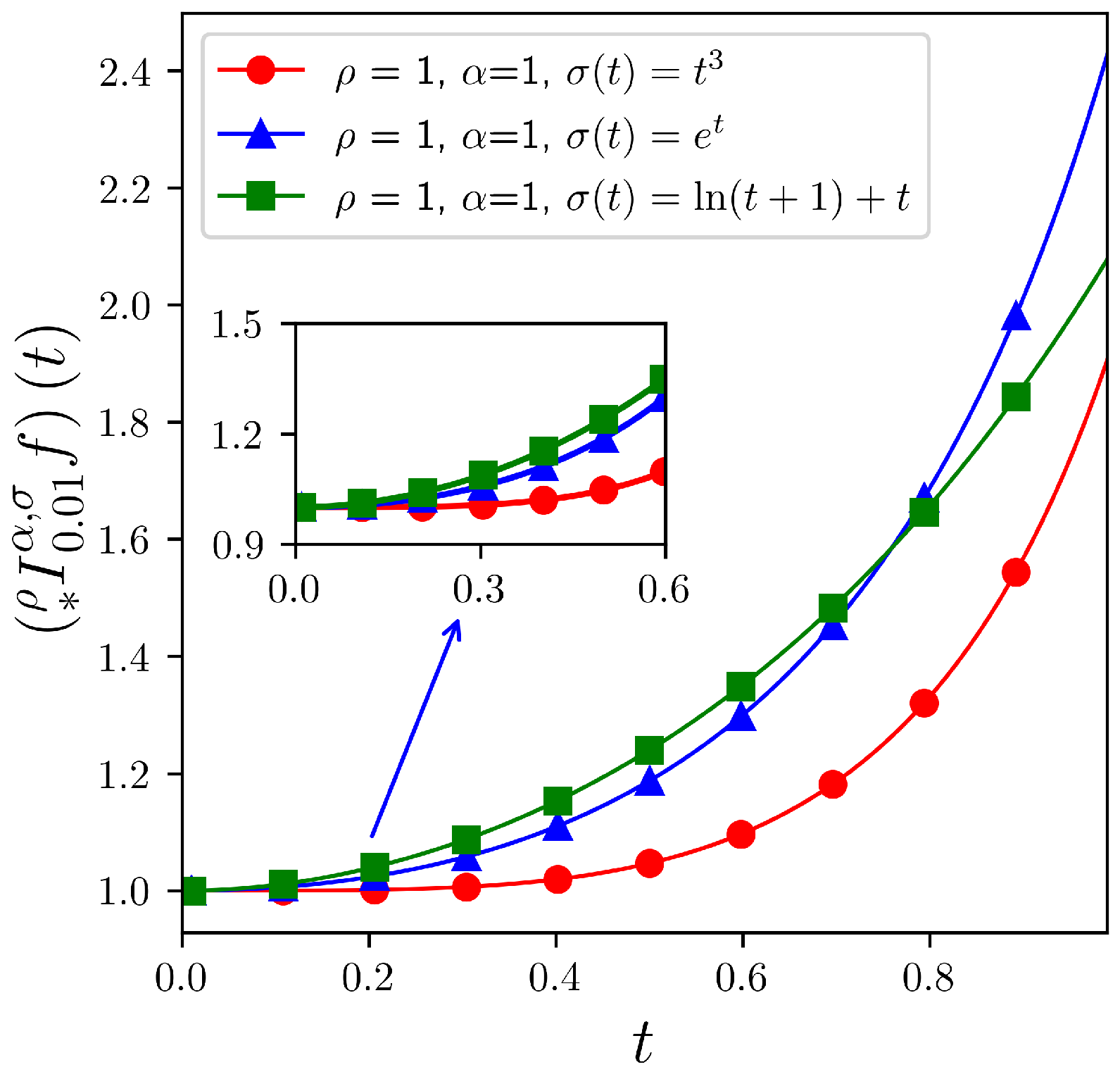
Remark 5.

For the convenience of expression below, the quantities are defined as follows:

$$\begin{array}{c}\hfill \Lambda (\rho ,\alpha ,t,s):={\displaystyle \frac{exp\left\{\frac{\rho -1}{\rho }(\sigma \left(t\right)-\sigma \left(s\right))\right\}}{{(\sigma \left(t\right)-\sigma \left(s\right))}^{1-\alpha }}},\Lambda (\rho ,\alpha ,s,t):={\displaystyle \frac{exp\left\{\frac{\rho -1}{\rho }(\sigma \left(s\right)-\sigma \left(t\right))\right\}}{{(\sigma \left(s\right)-\sigma \left(t\right))}^{1-\alpha }}}.\end{array}$$

Example 2.

Next, the performance of the left-sided operator ${}_{*}{}^{\rho }I_{{\mu }_1}^{\alpha ,\sigma }$ as formulated in Definition 7, focusing on its behavior when applied to separate functions $f\left(t\right)=exp\left\{\pi t\right\}$ on the interval $[0.01,0.99]$. Taking ${\mu }_1=0.01$, the following holds:

$$\left({}_{*}{}^{\rho }I_{0.01}^{\alpha ,\sigma }f\right)\left(t\right)=exp\left\{{\displaystyle \frac{1}{{\rho }^{\alpha }\Gamma \left(\alpha \right)}}{\int }_{0.01}^t\Lambda \left(\rho ,\alpha ,t,s\right){\sigma }^{\prime }\left(s\right)lnf\left(s\right)\mathrm{d}s\right\}.$$

Using graphical visualization, the simulation results presented in Figure 1, Figure 2 and Figure 3 indicate that the core parameters $\alpha$, $\rho$, and the specific forms of the function $\sigma$ exert a significant influence on the behavior of the left-sided operator ${}_{*}{}^{\rho }I_{{\mu }_1}^{\alpha ,\sigma }$. In particular, under the given conditions, smaller values of $\alpha$ and $\rho$ correspond to a faster growth rate of the integral of the function f with respect to the variable t. Furthermore, among the considered cases, when $\sigma$ is taken as an exponential function, the growth of the integral is the most rapid, highlighting the sensitivity of the operator’s behavior to the choice of transformation function $\sigma$.

Next, we conduct a deeper examination of the properties of the integral operator ${}_{*}{}^{\rho }I_{{\mu }_1}^{\alpha ,\sigma }$.

Theorem 4.

Suppose that the function $f:[{\mu }_1,{\mu }_2]\to {\mathbb{R}}^{+}$ with $0<{\mu }_1<{\mu }_2$ is continuous and $*$ integrable. Then, for any $\alpha >0$ and $\rho \in (0,1]$, the function $ln\left({}_{*}{}^{\rho }I_{{\mu }_1}^{\alpha ,\sigma }f\left(t\right)\right)$ is continuously defined on $[{\mu }_1,{\mu }_2]$.

Proof. 

Assume $x,y\in [{\mu }_1,{\mu }_2]$ with $x⩽y$, we have

$$\begin{array}{cc}\hfill & \left|ln\left({}_{*}{}^{\rho }I_{{\mu }_1}^{\alpha ,\sigma }f\left(y\right)\right)-ln\left({}_{*}{}^{\rho }I_{{\mu }_1}^{\alpha ,\sigma }f\left(x\right)\right)\right|\hfill \\ \hfill =& \left|{\displaystyle \frac{1}{{\rho }^{\alpha }\Gamma \left(\alpha \right)}}\left(\begin{array}{cc}\hfill & {\int }_{{\mu }_1}^x\Lambda \left(\rho ,\alpha ,y,s\right){\sigma }^{\prime }\left(s\right)lnf\left(s\right)\mathrm{d}s\hfill \\ \hfill & +{\int }_x^y\Lambda \left(\rho ,\alpha ,y,s\right){\sigma }^{\prime }\left(s\right)lnf\left(s\right)\mathrm{d}s\hfill \\ \hfill & -{\int }_{{\mu }_1}^x\Lambda \left(\rho ,\alpha ,x,s\right){\sigma }^{\prime }\left(s\right)lnf\left(s\right)\mathrm{d}s\hfill \end{array}\right)\right|\hfill \\ \hfill ⩽& \left|{\displaystyle \frac{1}{{\rho }^{\alpha }\Gamma \left(\alpha \right)}}{\int }_{{\mu }_1}^x\left[\Lambda \left(\rho ,\alpha ,y,s\right)-\Lambda \left(\rho ,\alpha ,x,s\right)\right]{\sigma }^{\prime }\left(s\right)lnf\left(s\right)\mathrm{d}s\right|\hfill \\ \hfill & +\left|{\displaystyle \frac{1}{{\rho }^{\alpha }\Gamma \left(\alpha \right)}}{\int }_x^y\Lambda \left(\rho ,\alpha ,y,s\right){\sigma }^{\prime }\left(s\right)lnf\left(s\right)\mathrm{d}s\right|\hfill \\ \hfill ⩽& {\displaystyle \frac{{\int }_{{\mu }_1}^x\left|\Lambda \left(\rho ,\alpha ,y,s\right)-\Lambda \left(\rho ,\alpha ,x,s\right)\right|\left|lnf\left(s\right)\right|{\sigma }^{\prime }\left(s\right)\mathrm{d}s+\left|\Lambda \left(\rho ,\alpha ,y,x\right)\right|{\int }_x^y\left|lnf\left(s\right)\right|{\sigma }^{\prime }\left(s\right)\mathrm{d}s}{{\rho }^{\alpha }\Gamma \left(\alpha \right)}}.\hfill \end{array}$$

Note that for a fixed $s\in [{\mu }_1,x]$, the function $\Lambda (\rho ,\alpha ,t,s)$ is continuous with respect to t, and when $x\to y$, we have

$$\begin{array}{c}\hfill \left|\Lambda (\rho ,\alpha ,y,s)-\Lambda (\rho ,\alpha ,x,s)\right|\to 0.\end{array}$$

Moreover, since $lnf\left(s\right){\sigma }^{\prime }\left(s\right)$ is continuously integrable, by the Dominated Convergence Theorem, we obtain

$$\begin{array}{c}\hfill {\int }_{{\mu }_1}^x\left|\Lambda (\rho ,\alpha ,y,s)-\Lambda (\rho ,\alpha ,x,s)\right|\left|lnf\left(s\right)\right|{\sigma }^{\prime }\left(s\right)\mathrm{d}s\to 0.\end{array}$$

Similarly, because f is continuous (so $lnf$ is bounded), ${\int }_x^y{\sigma }^{\prime }\left(s\right)\mathrm{d}s\to 0$, and $\Lambda (\rho ,\alpha ,y,s)$ is bounded on the compact set, we have

$$\begin{array}{c}\hfill {\int }_x^y\left|\Lambda (\rho ,\alpha ,y,s)\right|\left|lnf\left(s\right)\right|{\sigma }^{\prime }\left(s\right)\mathrm{d}s\to 0.\end{array}$$

Therefore, the overall estimated term tends to zero, indicating that:

$$\begin{array}{c}\hfill \underset{x\to y}{lim}\left|ln\left({}_{*}{}^{\rho }I_{{\mu }_1}^{\alpha ,\sigma }f\left(y\right)\right)-ln\left({}_{*}{}^{\rho }I_{{\mu }_1}^{\alpha ,\sigma }f\left(x\right)\right)\right|=0,\end{array}$$

that is, the conclusion holds. □

Theorem 5.

Let $f:[{\mu }_1,{\mu }_2]\to {\mathbb{R}}^{+}$ be a continuous function, where $0<{\mu }_1<{\mu }_2$. Also, let α, $\beta >0$ and $\rho \in (0,1]$. Then, for all $t\in [{\mu }_1,{\mu }_2]$, the following equality holds:

$$\begin{array}{cc}{}_{*}{}^{\rho }I_{{\mu }_1}^{\alpha ,\sigma }\left({}_{*}{}^{\rho }I_{{\mu }_1}^{\beta ,\sigma }f\right)\left(t\right)\hfill & =\left({}_{*}{}^{\rho }I_{{\mu }_1}^{\alpha +\beta ,\sigma }f\right)\left(t\right)={}_{*}{}^{\rho }I_{{\mu }_1}^{\beta ,\sigma }\left({}_{*}{}^{\rho }I_{{\mu }_1}^{\alpha ,\sigma }f\right)\left(t\right).\hfill \end{array}$$

Proof. 

By adopting the definition of the operator ${}_{*}{}^{\rho }I_{{\mu }_1}^{\alpha ,\sigma }$, while leveraging the continuity of the function f and Dirichlet’s formula, we can obtain

$$\begin{array}{c}{}_{*}{}^{\rho }I_{{\mu }_1}^{\alpha ,\sigma }\left({}_{*}{}^{\rho }I_{{\mu }_1}^{\beta ,\sigma }f\right)\left(t\right)\hfill \\ =exp\left\{{}^{\rho }I_{{{\mu }_1}^{+}}^{\alpha ,\sigma }ln\left({}_{*}{}^{\rho }I_{{\mu }_1}^{\beta ,\sigma }f\left(t\right)\right)\right\}\hfill \\ =exp\left\{{\displaystyle \frac{1}{{\rho }^{\alpha }\Gamma \left(\alpha \right)}}{\int }_{{\mu }_1}^t\Lambda (\rho ,\alpha ,t,s){\sigma }^{\prime }\left(s\right)ln\left({}_{*}{}^{\rho }I_{{\mu }_1}^{\beta ,\sigma }f\left(s\right)\right)\mathrm{d}s\right\}\hfill \\ =exp\left\{{\displaystyle \frac{{\int }_{{\mu }_1}^t\left({\int }_{{\mu }_1}^s\Lambda (\rho ,\beta ,s,u)lnf\left(u\right){\sigma }^{\prime }\left(u\right)\mathrm{d}u\right)\Lambda (\rho ,\alpha ,t,s){\sigma }^{\prime }\left(s\right)\mathrm{d}s}{{\rho }^{\alpha +\beta }\Gamma \left(\alpha \right)\Gamma \left(\beta \right)}}\right\}\hfill \\ =exp\left\{{\displaystyle \frac{{\int }_{{\mu }_1}^t\left({\int }_u^t\left[\Lambda (1,\alpha ,t,s)\Lambda (1,\beta ,s,u)\right]{\sigma }^{\prime }\left(s\right)\mathrm{d}s\right)\Lambda (\rho ,1,t,u)lnf\left(u\right){\sigma }^{\prime }\left(u\right)\mathrm{d}u}{{\rho }^{\alpha +\beta }\Gamma \left(\alpha \right)\Gamma \left(\beta \right)}}\right\}.\hfill \end{array}$$

(1)

Through the substitution of variable $y={\displaystyle \frac{\sigma \left(s\right)-\sigma \left(u\right)}{\sigma \left(t\right)-\sigma \left(u\right)}}$, we obtain

$$\begin{array}{c}{\int }_u^t[\Lambda (1,\alpha ,t,s)·\Lambda (1,\beta ,s,u)]{\sigma }^{\prime }\left(s\right)\mathrm{d}s\hfill \\ =\Lambda (1,\alpha +\beta ,t,u){\int }_0^1{(1-y)}^{\alpha -1}{y}^{\beta -1}\mathrm{d}y\hfill \\ ={\displaystyle \frac{\Gamma \left(\alpha \right)\Gamma \left(\beta \right)}{\Gamma (\alpha +\beta )}}\Lambda (1,\alpha +\beta ,t,u).\hfill \end{array}$$

(2)

Substituting Equation (2) into Equation (1), we have

$$\begin{array}{c}{}_{*}{}^{\rho }I_{{\mu }_1}^{\alpha ,\sigma }\left({}_{*}{}^{\rho }I_{{\mu }_1}^{\beta ,\sigma }f\right)\left(t\right)\hfill \\ =exp\left\{{\displaystyle \frac{1}{{\rho }^{\alpha +\beta }\Gamma (\alpha +\beta )}}{\int }_{{\mu }_1}^t\Lambda \left(\rho ,\alpha +\beta ,t,u\right)lnf\left(u\right){\sigma }^{\prime }\left(u\right)\mathrm{d}u\right\}\hfill \\ =\left({}_{*}{}^{\rho }I_{{\mu }_1}^{\alpha +\beta ,\sigma }f\right)\left(t\right).\hfill \end{array}$$

(3)

By reversing the values of $\alpha$ and $\beta$ in Equation (3), the second equation can be proven. □

Theorem 6.

Suppose that ${\mu }_1>0$, $\alpha >0$, $\beta >0$ and $\rho \in (0,1]$. Then, for all $t>{\mu }_1$, the following equation holds:

$$\begin{array}{c}\hfill {}_{*}{}^{\rho }I_{{\mu }_1}^{\alpha ,\sigma }\left[exp\left\{\Lambda \left(\rho ,\beta ,t,{\mu }_1\right)\right\}\right]=exp\left\{{\displaystyle \frac{\Gamma \left(\beta \right)\Lambda \left(\rho ,\alpha +\beta ,t,{\mu }_1\right)}{{\rho }^{\alpha }\Gamma (\alpha +\beta )}}\right\}.\end{array}$$

Proof. 

Through the substitution of variable $y={\displaystyle \frac{\sigma \left(t\right)-\sigma \left(s\right)}{\sigma \left(t\right)-\sigma \left({\mu }_1\right)}}$, we can obtain

$$\begin{array}{c}{}_{*}{}^{\rho }I_{{\mu }_1}^{\alpha ,\sigma }\left[exp\left\{\Lambda \left(\rho ,\beta ,t,{\mu }_1\right)\right\}\right]\hfill \\ =exp\left\{{\displaystyle \frac{1}{{\rho }^{\alpha }\Gamma \left(\alpha \right)}}{\int }_{{\mu }_1}^t\left[\Lambda \left(\rho ,\alpha ,t,s\right)·\Lambda \left(\rho ,\beta ,s,{\mu }_1\right)\right]{\sigma }^{\prime }\left(s\right)\mathrm{d}s\right\}\hfill \\ =exp\left\{{\displaystyle \frac{\Lambda \left(\rho ,\alpha +\beta ,t,{\mu }_1\right)}{{\rho }^{\alpha }\Gamma \left(\alpha \right)}}{\int }_0^1{(1-y)}^{\alpha -1}{y}^{\beta -1}\mathrm{d}y\right\}\hfill \\ =exp\left\{{\displaystyle \frac{\Gamma \left(\beta \right)\Lambda \left(\rho ,\alpha +\beta ,t,{\mu }_1\right)}{{\rho }^{\alpha }\Gamma (\alpha +\beta )}}\right\}.\hfill \end{array}$$

This completes the proof. □

Theorem 7.

Let f, $g:[{\mu }_1,{\mu }_2]\to {\mathbb{R}}^{+}$ be integrable functions, where $0<{\mu }_1<{\mu }_2$. For $\alpha >0$ and $\rho \in (0,1]$, the operator ${}_{*}{}^{\rho }I_{{\mu }_1}^{\alpha ,\sigma }$ has multiplicative linearity.

$$\begin{array}{c}\hfill {}_{*}{}^{\rho }I_{{\mu }_1}^{\alpha ,\sigma }\left(f^a·g^b\right)\left(t\right)={\left[{}_{*}{}^{\rho }I_{{\mu }_1}^{\alpha ,\sigma }f\left(t\right)\right]}^a{\left[{}_{*}{}^{\rho }I_{{\mu }_1}^{\alpha ,\sigma }g\left(t\right)\right]}^b.\end{array}$$

Proof. 

By leveraging the continuity of functions f and g, we obtain

$$\begin{array}{cc}\hfill {}_{*}{}^{\rho }I_{{\mu }_1}^{\alpha ,\sigma }\left(f^a·g^b\right)\left(t\right)& =exp\left\{{}^{\rho }I_{{{\mu }_1}^{+}}^{\alpha ,\sigma }ln\left(f^a·g^b\right)\left(t\right)\right\}\hfill \\ \hfill & =exp\left\{{\displaystyle \frac{1}{{\rho }^{\alpha }\Gamma \left(\alpha \right)}}{\int }_{{\mu }_1}^t\Lambda \left(\rho ,\alpha ,t,s\right)ln\left(f^a·g^b\right)\left(s\right){\sigma }^{\prime }\left(s\right)\mathrm{d}s\right\}\hfill \\ \hfill & =exp\left\{\begin{array}{c}{\displaystyle \frac{a}{{\rho }^{\alpha }\Gamma \left(\alpha \right)}}{\int }_{{\mu }_1}^t\Lambda \left(\rho ,\alpha ,t,s\right){\sigma }^{\prime }\left(s\right)lnf\left(s\right)\mathrm{d}s\hfill \\ +{\displaystyle \frac{b}{{\rho }^{\alpha }\Gamma \left(\alpha \right)}}{\int }_{{\mu }_1}^t\Lambda \left(\rho ,\alpha ,t,s\right){\sigma }^{\prime }\left(s\right)lng\left(s\right)\mathrm{d}s\hfill \end{array}\right\}\hfill \\ \hfill & ={\left[{}_{*}{}^{\rho }I_{{\mu }_1}^{\alpha ,\sigma }f\left(t\right)\right]}^a{\left[{}_{*}{}^{\rho }I_{{\mu }_1}^{\alpha ,\sigma }g\left(t\right)\right]}^b.\hfill \end{array}$$

This completes the proof. □

Theorem 8.

Assume that the function $f:[{\mu }_1,{\mu }_2]\to {\mathbb{R}}^{+}$ is integrable on $[{\mu }_1,{\mu }_2]$, where $0<{\mu }_1<{\mu }_2$ and $lnf$ is a bounded mapping on $[{\mu }_1,{\mu }_2]$. σ is a Lipschitz mapping and a monotonically increasing positive function on $[{\mu }_1,{\mu }_2]$, and has a continuous derivative ${\sigma }^{\prime }$ on $({\mu }_1,{\mu }_2)$. Then, for any $\alpha >0$, $\rho \in (0,1]$, $ln\left({}_{*}{}^{\rho }I_{{\mu }_1}^{\alpha ,\sigma }f\left(t\right)\right)$ is also a Lipschitz mapping on $[{\mu }_1,{\mu }_2]$.

Proof. 

Since $lnf$ is a bounded function, there exists a constant M, such that $|lnf(t\left)\right|\le M$. Assume that ${\mu }_1\le s\le u\le t\le {\mu }_2$. Using the monotonic increasing property of $\sigma$, we know that $0\le \left|exp\left\{{\displaystyle \frac{\rho -1}{\rho }}(\sigma \left(t\right)-\sigma \left(s\right))\right\}\right|\le 1$; therefore, we have

$$\begin{array}{c}\left|ln\left({}_{*}{}^{\rho }I_{{\mu }_1}^{\alpha ,\sigma }f\left(t\right)\right)-ln\left({}_{*}{}^{\rho }I_{{\mu }_1}^{\alpha ,\sigma }f\left(u\right)\right)\right|\hfill \\ \le {\displaystyle \frac{1}{{\rho }^{\alpha }\Gamma \left(\alpha \right)}}\left[\begin{array}{c}{\int }_{{\mu }_1}^t{\displaystyle \frac{\left|exp\left\{\frac{\rho -1}{\rho }(\sigma \left(t\right)-\sigma \left(s\right))\right\}\right|}{{(\sigma \left(t\right)-\sigma \left(s\right))}^{1-\alpha }}}|lnf\left(s\right)|{\sigma }^{\prime }\left(s\right)\mathrm{d}s\hfill \\ -{\int }_{{\mu }_1}^u{\displaystyle \frac{\left|exp\left\{\frac{\rho -1}{\rho }(\sigma \left(u\right)-\sigma \left(s\right))\right\}\right|}{{(\sigma \left(u\right)-\sigma \left(s\right))}^{1-\alpha }}}|lnf\left(s\right)|{\sigma }^{\prime }\left(s\right)\mathrm{d}s\hfill \end{array}\right]\hfill \\ \le {\displaystyle \frac{M}{{\rho }^{\alpha }\Gamma \left(\alpha \right)}}\left[\begin{array}{c}{\int }_{{\mu }_1}^u\left[{(\sigma \left(t\right)-\sigma \left(s\right))}^{\alpha -1}-{(\sigma \left(u\right)-\sigma \left(s\right))}^{\alpha -1}\right]{\sigma }^{\prime }\left(s\right)\mathrm{d}s\hfill \\ +{\int }_u^t{(\sigma \left(t\right)-\sigma \left(s\right))}^{\alpha -1}{\sigma }^{\prime }\left(s\right)\mathrm{d}s\hfill \\ +{\int }_{{\mu }_1}^u{\left(\sigma \left(u\right)-\sigma \left(s\right)\right)}^{\alpha -1}\left|\varphi \left({\Delta }_t\right)-\varphi \left({\Delta }_u\right)\right|{\sigma }^{\prime }\left(s\right)\mathrm{d}s\hfill \end{array}\right]\hfill \\ \le {\displaystyle \frac{M}{{\rho }^{\alpha }\Gamma (\alpha +1)}}\left[\begin{array}{c}\left({(\sigma \left(t\right)-\sigma \left({\mu }_1\right))}^{\alpha }-{(\sigma \left(u\right)-\sigma \left({\mu }_1\right))}^{\alpha }\right)\hfill \\ +{\displaystyle \frac{1-\rho }{\rho }}(\sigma \left(t\right)-\sigma \left(u\right)){(\sigma \left(u\right)-\sigma \left({\mu }_1\right))}^{\alpha }\hfill \end{array}\right],\hfill \end{array}$$

where

$$\left|\varphi \left({\Delta }_t\right)-\varphi \left({\Delta }_u\right)\right|=\left|exp\left\{{\displaystyle \frac{\rho -1}{\rho }}\left(\sigma \left(t\right)-\sigma \left(s\right)\right)\right\}-exp\left\{{\displaystyle \frac{\rho -1}{\rho }}\left(\sigma \left(u\right)-\sigma \left(s\right)\right)\right\}\right|.$$

Since $\sigma$ is a monotonically increasing positive function on $[{\mu }_1,{\mu }_2]$ and has a continuous derivative ${\sigma }^{\prime }$ on $({\mu }_1,{\mu }_2)$, we know that $\sigma \left(t\right)-\sigma \left({\mu }_1\right)>0$ and $\sigma \left(u\right)-\sigma \left({\mu }_1\right)>0$. For any $\alpha >0$, let $h\left(x\right)=x^{\alpha }$ on $[\sigma \left(u\right)-\sigma \left({\mu }_1\right),\sigma \left(t\right)-\sigma \left({\mu }_1\right)]$. Then, $h\left(x\right)$ satisfies the conditions of the Lagrange mean value theorem, that is, we obtain

$${(\sigma \left(t\right)-\sigma \left({\mu }_1\right))}^{\alpha }-{(\sigma \left(u\right)-\sigma \left({\mu }_1\right))}^{\alpha }=\alpha {(\sigma \left(\xi \right)-\sigma \left({\mu }_1\right))}^{\alpha -1}(\sigma \left(t\right)-\sigma \left(u\right)).$$

Since $\sigma$ is a Lipschitz function on $[{\mu }_1,{\mu }_2]$, for $\forall t,u\in [{\mu }_1,{\mu }_2]$, There exist positive constants $L_1$, $L_2$, and L such that $L⩾{\displaystyle \frac{1-\rho }{\rho }}{L}_1{\left(L_2\right)}^{\alpha }$ and $L⩾L_1$. Then $\left|\sigma \left(t\right)-\sigma \left(u\right)\right|⩽L_1\left|t-u\right|$ and $\left|\sigma \left(u\right)-\sigma \left({\mu }_1\right)\right|⩽L_2\left|u-{\mu }_1\right|$; therefore, we obtain

$$\begin{array}{c}\left|ln\left({}_{*}{}^{\rho }I_{{\mu }_1}^{\alpha ,\sigma }f\left(t\right)\right)-ln\left({}_{*}{}^{\rho }I_{{\mu }_1}^{\alpha ,\sigma }f\left(u\right)\right)\right|\hfill \\ ⩽{\displaystyle \frac{M}{{\rho }^{\alpha }\Gamma \left(\alpha \right)}}\left[\begin{array}{c}{L}_1{\left(\sigma \left(\xi \right)-\sigma \left({\mu }_1\right)\right)}^{\alpha -1}\left|t-u\right|\\ +{\displaystyle \frac{1-\rho }{\rho }}{L}_1{\left(L_2\right)}^{\alpha }\left|t-u\right|{\left|u-{\mu }_1\right|}^{\alpha }\end{array}\right]\hfill \\ ⩽{\displaystyle \frac{ML}{{\rho }^{\alpha }\Gamma \left(\alpha \right)}}\left({\left(\sigma \left({\mu }_2\right)-\sigma \left({\mu }_1\right)\right)}^{\alpha -1}+{\left(u-{\mu }_1\right)}^{\alpha }\right)\left|t-u\right|.\hfill \end{array}$$

This establishes the desired result and the proof is complete. □

To prove the boundedness of $ln\left({}_{*}{}^{\rho }I_{{\mu }_1}^{\alpha ,\sigma }f\right)$ in the space $X_{\sigma }^p({\mu }_1,{\mu }_2)$ for $1\le p\le \infty$, it is essential to re-examine the definition of the norm ${\parallel ·\parallel }_{X_{\sigma }^p}$.

Definition 8

([44]). Let $f\in L_1[{\mu }_1,{\mu }_2]$ and let σ be an increasing, positive and monotone function on $[{\mu }_1,{\mu }_2]$ with a continuous derivative ${\sigma }^{\prime }$ for $0<{\mu }_1\le s\le {\mu }_2<\infty$. For $1\le p<\infty$, the space $X_{\sigma }^p({\mu }_1,{\mu }_2)$ is defined as the set of all real-valued, Lebesgue measurable functions f on $[{\mu }_1,{\mu }_2]$ and its norm is given by

$${\parallel f\parallel }_{X_{\sigma }^p}={\left({\int }_{{\mu }_1}^{{\mu }_2}{\left|f\left(s\right)\right|}^p{\sigma }^{\prime }\left(s\right)\mathrm{d}s\right)}^{{\displaystyle \frac{1}{p}}}<\infty .$$

Theorem 9.

Suppose that the function $f:[{\mu }_1,{\mu }_2]\to {\mathbb{R}}^{+}$ is integrable. Given $\alpha >0$, $\rho \in (0,1]$, $1\le p<\infty$ and $f\in X_{\sigma }^p({\mu }_1,{\mu }_2)$. Then $ln\left({}_{*}{}^{\rho }I_{{\mu }_1}^{\alpha ,\sigma }f\right)$ is bounded in $X_{\sigma }^p({\mu }_1,{\mu }_2)$, and

$${∥ln\left({}_{*}{}^{\rho }I_{{\mu }_1}^{\alpha ,\sigma }f\right)∥}_{X_{\sigma }^p}\le {\left({\displaystyle \frac{q\alpha }{p(\alpha -1)+1}}\right)}^{{\displaystyle \frac{1}{p}}}{\displaystyle \frac{{(\sigma \left({\mu }_2\right)-\sigma \left({\mu }_1\right))}^{\alpha }{∥lnf∥}_{X_{\sigma }^p}}{q{\rho }^{\alpha }\Gamma (\alpha +1)}}.$$

Proof. 

For $1<p<\infty$ and $t_2>t_1$, we have

$$\begin{array}{cc}\hfill {∥ln\left({}_{*}{}^{\rho }I_{{\mu }_1}^{\alpha ,\sigma }f\right)∥}_{X_{\sigma }^p}& ={\left({\int }_{{\mu }_1}^{{\mu }_2}{\left|ln\left({}_{*}{}^{\rho }I_{{\mu }_1}^{\alpha ,\sigma }f\right)\right|}^p{\sigma }^{\prime }\left(t\right)\mathrm{d}t\right)}^{{\displaystyle \frac{1}{p}}}\hfill \\ \hfill & ={\displaystyle \frac{1}{{\rho }^{\alpha }\Gamma \left(\alpha \right)}}{\left({\int }_{{\mu }_1}^{{\mu }_2}{\left|{\int }_{{\mu }_1}^t\Lambda \left(\rho ,\alpha ,t,s\right)lnf\left(s\right){\sigma }^{\prime }\left(s\right)\mathrm{d}s\right|}^p{\sigma }^{\prime }\left(t\right)\mathrm{d}t\right)}^{{\displaystyle \frac{1}{p}}}\hfill \\ \hfill & ={\displaystyle \frac{1}{{\rho }^{\alpha }\Gamma \left(\alpha \right)}}{\left({\int }_{\sigma \left({\mu }_1\right)}^{\sigma \left({\mu }_2\right)}{\left|{\int }_{\sigma \left({\mu }_1\right)}^{t_2}{\displaystyle \frac{exp\left\{\frac{\rho -1}{\rho }(t_2-t_1)\right\}}{{(t_2-t_1)}^{1-\alpha }}}lnf\left({\sigma }^{-1}\left(t_1\right)\right)\mathrm{d}{t}_1\right|}^p\mathrm{d}{t}_2\right)}^{{\displaystyle \frac{1}{p}}}.\hfill \end{array}$$

Using the fact that $0\le \left|exp\left\{{\displaystyle \frac{\rho -1}{\rho }}(t_2-t_1)\right\}\right|\le 1$ and taking into account the generalized Minkowski inequality ([45]), we have

$$\begin{array}{cc}\hfill {∥ln\left({}_{*}{}^{\rho }I_{{\mu }_1}^{\alpha ,\sigma }f\right)∥}_{X_{\sigma }^p}& \le {\displaystyle \frac{1}{{\rho }^{\alpha }\Gamma \left(\alpha \right)}}{\int }_{\sigma \left({\mu }_1\right)}^{\sigma \left({\mu }_2\right)}{\left({\left|lnf\left({\sigma }^{-1}\left(t_1\right)\right)\right|}^p{\int }_{t_1}^{\sigma \left({\mu }_2\right)}{(t_2-t_1)}^{p(\alpha -1)}d{t}_2\right)}^{{\displaystyle \frac{1}{p}}}\mathrm{d}{t}_1\hfill \\ \hfill & ={\displaystyle \frac{1}{{\rho }^{\alpha }\Gamma \left(\alpha \right)}}{\int }_{\sigma \left({\mu }_1\right)}^{\sigma \left({\mu }_2\right)}\left|lnf\left({\sigma }^{-1}\left(t_1\right)\right)\right|{\left({\displaystyle \frac{{(\sigma \left({\mu }_2\right)-t_1)}^{p(\alpha -1)+1}}{p(\alpha -1)+1}}\right)}^{{\displaystyle \frac{1}{p}}}\mathrm{d}{t}_1.\hfill \end{array}$$

By employing the well-known Hölder inequality with ${\displaystyle \frac{1}{p}}+{\displaystyle \frac{1}{q}}=1$, we can obtain

$$\begin{array}{cc}\hfill {∥ln\left({}_{*}{}^{\rho }I_{{\mu }_1}^{\alpha ,\sigma }f\right)∥}_{X_{\sigma }^p}& \le {\displaystyle \frac{1}{{\rho }^{\alpha }\Gamma \left(\alpha \right)}}{\left({\int }_{\sigma \left({\mu }_1\right)}^{\sigma \left({\mu }_2\right)}{\left|lnf\left({\sigma }^{-1}\left(t_1\right)\right)\right|}^p\mathrm{d}{t}_1\right)}^{{\displaystyle \frac{1}{p}}}\hfill \\ \hfill & \times {\left({\int }_{\sigma \left({\mu }_1\right)}^{\sigma \left({\mu }_2\right)}{\left({\displaystyle \frac{{(\sigma \left({\mu }_2\right)-t_1)}^{p(\alpha -1)+1}}{p(\alpha -1)+1}}\right)}^{{\displaystyle \frac{q}{p}}}\mathrm{d}{t}_1\right)}^{{\displaystyle \frac{1}{q}}}\hfill \\ \hfill & ={\left({\displaystyle \frac{q\alpha }{p(\alpha -1)+1}}\right)}^{{\displaystyle \frac{1}{p}}}{\displaystyle \frac{{(\sigma \left({\mu }_2\right)-\sigma \left({\mu }_1\right))}^{\alpha }{∥lnf∥}_{X_{\sigma }^p}}{q{\rho }^{\alpha }\Gamma (\alpha +1)}}.\hfill \end{array}$$

This completes the proof. □

Remark 6.

The operator ${}_{{\mu }_2}I_{*}^{\alpha ,\sigma ,\rho }$ yields results that are similar to those presented above.

5. The Hermite–Hadamard Inequality of the Multiplicative Fractional Integrals

The following presents the derivation of Hermite–Hadamard type inequalities for multiplicative generalized proportional $\sigma$-Riemann–Liouville fractional integrals via multiplicative $\sigma$-convex functions. Compared with the classical multiplicative Riemann–Liouville operator, the generalized form introduced here provides broader generality and greater applicability, thereby extending the scope and flexibility of related integral inequalities.

Definition 9

([19]). For $\vartheta >\theta >0$, the confluent hypergeometric function admits an integral representation given by

$${}_{1}F_1(\theta ,\vartheta ,x)={\displaystyle \frac{\Gamma \left(\vartheta \right)}{\Gamma (\vartheta -\theta )\Gamma \left(\theta \right)}}{\int }_0^1\exp \left\{xt\right\}{t}^{\theta -1}{(1-t)}^{\vartheta -\theta -1}\mathrm{d}t.$$

Theorem 10.

Let f be a positive function that is multiplicatively σ-convex on $[{\mu }_1,{\mu }_2]$ with $0<{\mu }_1<{\mu }_2$, σ is a monotonically increasing positive function on $[{\mu }_1,{\mu }_2]$, and has a continuous derivative ${\sigma }^{\prime }$ on $({\mu }_1,{\mu }_2)$. For $\alpha >0$ and $\rho \in (0,1]$, the following Hermite–Hadamard inequality for multiplicative generalized proportional σ-Riemann–Liouville fractional integrals holds:

$$\begin{array}{c}f\left({\sigma }^{-1}\left({\displaystyle \frac{\sigma \left({\mu }_1\right)+\sigma \left({\mu }_2\right)}{2}}\right)\right)\hfill \\ \le {\left[{}_{{\mu }_2}I_{*}^{\alpha ,\sigma ,\rho }f\left({\mu }_1\right)·{}_{*}{}^{\rho }I_{{\mu }_1}^{\alpha ,\sigma }f\left({\mu }_2\right)\right]}^{{\displaystyle \frac{{\rho }^{\alpha }\Gamma (\alpha +1)}{2{(\sigma \left({\mu }_2\right)-\sigma \left({\mu }_1\right))}^{\alpha }{}_{1}F_1\left(\alpha ,\alpha +1,\frac{\rho -1}{\rho }(\sigma \left({\mu }_2\right)-\sigma \left({\mu }_1\right))\right)}}}\hfill \\ \le \sqrt{f\left({\mu }_1\right)f\left({\mu }_2\right)}.\hfill \end{array}$$

Proof. 

Since f is a positive and multiplicatively $\sigma$-convex function on $[{\mu }_1,{\mu }_2]$, we can obtain

$$\begin{array}{cc}\hfill lnf\left({\sigma }^{-1}\left({\displaystyle \frac{\sigma \left({\mu }_1\right)+\sigma \left({\mu }_2\right)}{2}}\right)\right)& \le {\displaystyle \frac{1}{2}}\left[\begin{array}{c}lnf\left({\sigma }^{-1}\left((1-t)\sigma \left({\mu }_1\right)+t\sigma \left({\mu }_2\right)\right)\right)\hfill \\ +lnf\left({\sigma }^{-1}\left(t\sigma \left({\mu }_1\right)+(1-t)\sigma \left({\mu }_2\right)\right)\right)\hfill \end{array}\right].\hfill \end{array}$$

(4)

After the inequality (4) is multiplied by ${\displaystyle \frac{t^{\alpha -1}}{{\rho }^{\alpha }\Gamma \left(\alpha \right)}}exp\left\{{\displaystyle \frac{\rho -1}{\rho }}t(\sigma \left({\mu }_2\right)-\sigma \left({\mu }_1\right))\right\}$ and the resulting inequality is integrated with respect to t over the interval $[0,1]$, we obtain

$$\begin{array}{c}{\displaystyle \frac{2}{{\rho }^{\alpha }\Gamma \left(\alpha \right)}}lnf\left({\sigma }^{-1}\left({\displaystyle \frac{\sigma \left({\mu }_1\right)+\sigma \left({\mu }_2\right)}{2}}\right)\right){\int }_0^1{t}^{\alpha -1}exp\left\{{\displaystyle \frac{\rho -1}{\rho }}t(\sigma \left({\mu }_2\right)-\sigma \left({\mu }_1\right))\right\}\mathrm{d}t\hfill \\ \le {\displaystyle \frac{1}{{\rho }^{\alpha }\Gamma \left(\alpha \right)}}{\int }_0^1{t}^{\alpha -1}exp\left\{{\displaystyle \frac{\rho -1}{\rho }}t(\sigma \left({\mu }_2\right)-\sigma \left({\mu }_1\right))\right\}lnf\left({\sigma }^{-1}\left((1-t)\sigma \left({\mu }_1\right)+t\sigma \left({\mu }_2\right)\right)\right)\mathrm{d}t\hfill \\ +{\displaystyle \frac{1}{{\rho }^{\alpha }\Gamma \left(\alpha \right)}}{\int }_0^1{t}^{\alpha -1}exp\left\{{\displaystyle \frac{\rho -1}{\rho }}t(\sigma \left({\mu }_2\right)-\sigma \left({\mu }_1\right))\right\}lnf\left({\sigma }^{-1}\left(t\sigma \left({\mu }_1\right)+(1-t)\sigma \left({\mu }_2\right)\right)\right)\mathrm{d}t\hfill \\ ={\displaystyle \frac{1}{{(\sigma \left({\mu }_2\right)-\sigma \left({\mu }_1\right))}^{\alpha }}}\left[{}^{\rho }I_{{{\mu }_1}^{+}}^{\alpha ,\sigma }lnf\left({\mu }_2\right)+{}^{\rho }I_{{{\mu }_2}^{-}}^{\alpha ,\sigma }lnf\left({\mu }_1\right)\right].\hfill \end{array}$$

Moreover, because

$$\begin{array}{cc}\hfill \alpha {\int }_0^1{t}^{\alpha -1}exp\left\{{\displaystyle \frac{\rho -1}{\rho }}t(\sigma \left({\mu }_2\right)-\sigma \left({\mu }_1\right))\right\}\mathrm{d}t& ={}_{1}F_1\left(\alpha ,\alpha +1,{\displaystyle \frac{\rho -1}{\rho }}(\sigma \left({\mu }_2\right)-\sigma \left({\mu }_1\right))\right).\hfill \end{array}$$

Therefore, we have

$$\begin{array}{cc}\hfill lnf\left({\sigma }^{-1}\left({\displaystyle \frac{\sigma \left({\mu }_1\right)+\sigma \left({\mu }_2\right)}{2}}\right)\right)& \le {\displaystyle \frac{{\rho }^{\alpha }\Gamma (\alpha +1)\left[{}^{\rho }I_{{{\mu }_1}^{+}}^{\alpha ,\sigma }lnf\left({\mu }_2\right)+{}^{\rho }I_{{{\mu }_2}^{-}}^{\alpha ,\sigma }lnf\left({\mu }_1\right)\right]}{2{(\sigma \left({\mu }_2\right)-\sigma \left({\mu }_1\right))}^{\alpha }{}_{1}F_1\left(\alpha ,\alpha +1,\frac{\rho -1}{\rho }(\sigma \left({\mu }_2\right)-\sigma \left({\mu }_1\right))\right)}}.\hfill \end{array}$$

Thus, we can obtain

$$\begin{array}{cc}\hfill f\left({\sigma }^{-1}\left({\displaystyle \frac{\sigma \left({\mu }_1\right)+\sigma \left({\mu }_2\right)}{2}}\right)\right)& \le {\left[{}_{{\mu }_2}I_{*}^{\alpha ,\sigma ,\rho }f\left({\mu }_1\right)·{}_{*}{}^{\rho }I_{{\mu }_1}^{\alpha ,\sigma }f\left({\mu }_2\right)\right]}^{{\displaystyle \frac{{\rho }^{\alpha }\Gamma (\alpha +1)}{2{(\sigma \left({\mu }_2\right)-\sigma \left({\mu }_1\right))}^{\alpha }{}_{1}F_1\left(\alpha ,\alpha +1,\frac{\rho -1}{\rho }(\sigma \left({\mu }_2\right)-\sigma \left({\mu }_1\right))\right)}}}.\hfill \end{array}$$

Since f is a multiplicatively $\sigma$-convex function on the interval $[{\mu }_1,{\mu }_2]$, we obtain

$$\begin{array}{cc}\hfill f\left({\sigma }^{-1}\left((1-t)\sigma \left({\mu }_1\right)+t\sigma \left({\mu }_2\right)\right)\right)& \le {\left[f\left({\mu }_2\right)\right]}^t{\left[f\left({\mu }_1\right)\right]}^{1-t},\hfill \\ \hfill f\left({\sigma }^{-1}\left(t\sigma \left({\mu }_1\right)+(1-t)\sigma \left({\mu }_2\right)\right)\right)& \le {\left[f\left({\mu }_1\right)\right]}^t{\left[f\left({\mu }_2\right)\right]}^{1-t}.\hfill \end{array}$$

As a consequence, the following inequality holds:

$$\begin{array}{cc}\hfill & lnf\left({\sigma }^{-1}\left(\left(1-t\right)\sigma \left({\mu }_1\right)+t\sigma \left({\mu }_2\right)\right)\right)+lnf\left({\sigma }^{-1}\left(t\sigma \left({\mu }_1\right)+\left(1-t\right)\sigma \left({\mu }_2\right)\right)\right)\hfill \\ \hfill & \le lnf\left({\mu }_1\right)+lnf\left({\mu }_2\right).\hfill \end{array}$$

(5)

After the inequality (5) is multiplied on both sides by ${\displaystyle \frac{t^{\alpha -1}}{{\rho }^{\alpha }\Gamma \left(\alpha \right)}}exp\left\{{\displaystyle \frac{\rho -1}{\rho }}t(\sigma \left({\mu }_2\right)-\sigma \left({\mu }_1\right))\right\}$ and the resulting inequality is integrated with respect to t over the interval $[0,1]$, we have

$$\begin{array}{c}{\displaystyle \frac{1}{{(\sigma \left({\mu }_2\right)-\sigma \left({\mu }_1\right))}^{\alpha }}}\left[{}^{\rho }I_{{{\mu }_1}^{+}}^{\alpha ,\sigma }lnf\left({\mu }_2\right)+{}^{\rho }I_{{{\mu }_2}^{-}}^{\alpha ,\sigma }lnf\left({\mu }_1\right)\right]\hfill \\ \le {\displaystyle \frac{lnf\left({\mu }_1\right)+lnf\left({\mu }_2\right)}{{\rho }^{\alpha }\Gamma \left(\alpha \right)}}{\int }_0^1{t}^{\alpha -1}exp\left\{{\displaystyle \frac{\rho -1}{\rho }}t(\sigma \left({\mu }_2\right)-\sigma \left({\mu }_1\right))\right\}\mathrm{d}t\hfill \\ ={\displaystyle \frac{lnf\left({\mu }_1\right)+lnf\left({\mu }_2\right)}{{\rho }^{\alpha }\Gamma (\alpha +1)}}{}_{1}F_1\left(\alpha ,\alpha +1,{\displaystyle \frac{\rho -1}{\rho }}(\sigma \left({\mu }_2\right)-\sigma \left({\mu }_1\right))\right).\hfill \end{array}$$

Therefore, we can obtain

$${\left[{}_{{\mu }_2}I_{*}^{\alpha ,\sigma ,\rho }f\left({\mu }_1\right)·{}_{*}{}^{\rho }I_{{\mu }_1}^{\alpha ,\sigma }f\left({\mu }_2\right)\right]}^{{\displaystyle \frac{{\rho }^{\alpha }\Gamma (\alpha +1)}{2{(\sigma \left({\mu }_2\right)-\sigma \left({\mu }_1\right))}^{\alpha }{}_{1}F_1\left(\alpha ,\alpha +1,\frac{\rho -1}{\rho }(\sigma \left({\mu }_2\right)-\sigma \left({\mu }_1\right))\right)}}}\le \sqrt{f\left({\mu }_1\right)f\left({\mu }_2\right)}.$$

Thus, the desired assertion is proven, completing the proof. □

Corollary 1.

Taking into account Theorem 10, when $\sigma \left(x\right)=x,\rho =1$, Budak and Özçelik [29] establish the Hermite–Hadamard inequality for multiplicatively convex functions as follows:

$$f\left({\displaystyle \frac{{\mu }_1+{\mu }_2}{2}}\right)\le {\left[{}_{{\mu }_1}I_{*}^{\alpha }f\left({\mu }_2\right)·{}_{*}I_{{\mu }_2}^{\alpha }f\left({\mu }_1\right)\right]}^{{\displaystyle \frac{\Gamma (\alpha +1)}{2{({\mu }_2-{\mu }_1)}^{\alpha }}}}\le \sqrt{f\left({\mu }_1\right)f\left({\mu }_2\right)}.$$

Corollary 2.

Taking into account Theorem 10, when $\rho =1$, $\sigma \left(x\right)=lnx$, Zhou and Du [34] examined the multiplicative Hadamard fractional integrals related to Hermite–Hadamard inequalities as follows:

$$f\left(\sqrt{{\mu }_1{\mu }_2}\right)⩽{\left[{}_{{\mu }_1}I_{*}^{\alpha }f\left({\mu }_2\right)·{}_{*}I_{{\mu }_2}^{\alpha }f\left({\mu }_1\right)\right]}^{{\displaystyle \frac{\Gamma \left(\alpha +1\right)}{2{\left(ln{\mu }_2-ln{\mu }_1\right)}^{\alpha }}}}⩽\sqrt{f\left({\mu }_1\right)f\left({\mu }_2\right)}.$$

Corollary 3.

Taking into account Theorem 10, when $\alpha =1,\rho =1$, we establish the Hermite–Hadamard inequality for integer-order integrals of multiplicative σ-convex functions.

$$f\left({\sigma }^{-1}\left({\displaystyle \frac{\sigma \left({\mu }_1\right)+\sigma \left({\mu }_2\right)}{2}}\right)\right)\le {\left({\int }_{{\mu }_1}^{{\mu }_2}{\left[f{\left(x\right)}^{{\sigma }^{\prime }\left(x\right)}\right]}^{\mathrm{d}x}\right)}^{{\displaystyle \frac{1}{\sigma \left({\mu }_2\right)-\sigma \left({\mu }_1\right)}}}\le \sqrt{f\left({\mu }_1\right)f\left({\mu }_2\right)}.$$

Corollary 4.

Suppose that for $i=1,2,\dots ,n$, the functions $f_i$ are positive and multiplicatively σ-convex on $[{\mu }_1,{\mu }_2]$, where $0<{\mu }_1<{\mu }_2$. Then,

$$\begin{array}{c}\prod _{i=1}^n{f}_i\left({\sigma }^{-1}\left({\displaystyle \frac{\sigma \left({\mu }_1\right)+\sigma \left({\mu }_2\right)}{2}}\right)\right)\hfill \\ \le {\left[{}_{{\mu }_2}I_{*}^{\alpha ,\sigma ,\rho }\left(\prod _{i=1}^n{f}_i\left({\mu }_1\right)\right)·{}_{*}{}^{\rho }I_{{\mu }_1}^{\alpha ,\sigma }\left(\prod _{i=1}^n{f}_i\left({\mu }_2\right)\right)\right]}^{{\displaystyle \frac{{\rho }^{\alpha }\Gamma (\alpha +1)}{2{(\sigma \left({\mu }_2\right)-\sigma \left({\mu }_1\right))}^{\alpha }{}_{1}F_1\left(\alpha ,\alpha +1,\frac{\rho -1}{\rho }(\sigma \left({\mu }_2\right)-\sigma \left({\mu }_1\right))\right)}}}\hfill \\ \le \prod _{i=1}^n\sqrt{f_i\left({\mu }_1\right)f_i\left({\mu }_2\right)}.\hfill \end{array}$$

Proof. 

Since the functions $f_i$ ($i=1,2,\dots ,n$) are positive and multiplicatively $\sigma$-convex on the interval $[{\mu }_1,{\mu }_2]$ with $0<{\mu }_1<{\mu }_2$, their product ${\prod }_{i=1}^n{f}_i$ is also positive and multiplicatively $\sigma$-convex. Therefore, by applying Theorem 10 to the function ${\prod }_{i=1}^n{f}_i$, we obtain the desired result. □

As illustrated in Example 1, a function of the form $f\left(x\right)=exp\left\{g\right(\sigma \left(x\right)\left)\right\}$, where $g\left(x\right)$ is convex and $\sigma$ is a strictly monotonic and continuous function, qualifies as a multiplicative $\sigma$-convex function. Building upon this foundation, we employ the numerical examples presented in Remarks 2 and 3 to provide a numerical verification of the validity of Theorem 10.

Example 3.

Let $\sigma \left(x\right)=lnx$, $x>1$, $g\left(y\right)=y^2$, $y\in \mathbb{R}$. Then $f\left(x\right)=exp\left\{{(lnx)}^2\right\}$. Also, assume ${\mu }_1=2$, ${\mu }_2=3$. Here, Theorem 10 is equivalent to

$$\begin{array}{c}exp\left\{{\left(ln\sqrt{6}\right)}^2\right\}\hfill \\ \le exp\left\{{\displaystyle \frac{\begin{array}{c}{\int }_2^3\frac{1}{s}{(lns)}^2{\left(ln\frac{s}{2}\right)}^{\alpha -1}{\left(\frac{s}{2}\right)}^{\left(\frac{\rho -1}{\rho }\right)}\mathrm{d}s\hfill \\ +{\int }_2^3\frac{1}{s}{(lns)}^2{\left(ln\frac{3}{s}\right)}^{\alpha -1}{\left(\frac{3}{s}\right)}^{\left(\frac{\rho -1}{\rho }\right)}\mathrm{d}s\hfill \end{array}}{2{\left(ln\frac{3}{2}\right)}^{\alpha }{\int }_0^1{t}^{\alpha -1}{\left(\frac{3}{2}\right)}^{\left(\frac{\rho -1}{\rho }\right)t}\mathrm{d}t}}\right\}\hfill \\ \le \sqrt{exp\left\{{(ln2)}^2+{(ln3)}^2\right\}}.\hfill \end{array}$$

(6)

Based on Example 3, we consider the parameter ranges $\alpha \in [0.1,0.99]$ and $\rho \in [0.1,0.99]$. Using graphical visualization techniques, we present Figure 4, which illustrates the plots of three functions corresponding to the left-hand side, middle term, and right-hand side of inequality (6). From Figure 4, it is evident that variations in the parameters $\alpha$ and $\rho$ result in distinct changes in the shapes and trajectories of the graphs. These changes highlight the significant impact of the parameters on the behavior of the inequality, emphasizing their essential role in shaping the underlying functional relationships.

Remark 7.

In Example 3, when assuming $\rho =1$, then the fractional integral in Theorem 10 becomes the Hadamard fractional integral. Here, Example 3 is tantamount to

$$\begin{array}{c}exp\left\{{\left(ln\sqrt{6}\right)}^2\right\}\hfill \\ \le exp\left\{{\displaystyle \frac{\alpha }{2}}{\left(ln{\displaystyle \frac{3}{2}}\right)}^{-\alpha }\left({\int }_2^3{\displaystyle \frac{1}{s}}{(lns)}^2{\left(ln{\displaystyle \frac{s}{2}}\right)}^{\alpha -1}\mathrm{d}s+{\int }_2^3{\displaystyle \frac{1}{s}}{(lns)}^2{\left(ln{\displaystyle \frac{3}{s}}\right)}^{\alpha -1}\mathrm{d}s\right)\right\}\hfill \\ \le \sqrt{exp\left\{{(ln2)}^2+{(ln3)}^2\right\}}.\hfill \end{array}$$

(7)

In contrast to Example 3, we now disregard the influence of the proportional parameter $\rho$ as discussed in Remark 7, and consider the variable $\alpha \in [0.1,0.99]$. Using graphical visualization, Figure 5 illustrates the graphs of the three functions corresponding to the left-hand side, middle, and right-hand side of inequality (7). This comparison highlights the significant regulatory role of the parameter $\rho$. As previously illustrated in Figure 4, incorporating $\rho$ introduces increased complexity and variability in the functional behavior. In contrast, omitting $\rho$ results in a simplified relationship among the functions, revealing its pivotal influence on the dynamic structure of the inequality.

Remark 8.

In Example 3, when we assume $\alpha =1$, the fractional integral in Theorem 10 is transformed into the proportional integral, and consequently, Example 3 is changed into

$$\begin{array}{c}exp\left\{{\left(ln\sqrt{6}\right)}^2\right\}\hfill \\ \le exp\left\{{\displaystyle \frac{\rho -1}{2\rho \left({\left(\frac{3}{2}\right)}^{\frac{\rho -1}{\rho }}-1\right)}}\left({\int }_2^3{\displaystyle \frac{1}{s}}{(lns)}^2{\left({\displaystyle \frac{s}{2}}\right)}^{{\displaystyle \frac{\rho -1}{\rho }}}\mathrm{d}s+{\int }_2^3{\displaystyle \frac{1}{s}}{(lns)}^2{\left({\displaystyle \frac{3}{s}}\right)}^{{\displaystyle \frac{\rho -1}{\rho }}}\mathrm{d}s\right)\right\}\hfill \\ \le \sqrt{exp\left\{{(ln2)}^2+{(ln3)}^2\right\}}.\hfill \end{array}$$

(8)

To further investigate the isolated influence of the proportional parameter $\rho$, we fix all other variables and allow $\rho$ to vary within the interval $[0.1,0.99]$. Utilizing graphical visualization, Figure 6 presents the plots of the three functions derived from inequality (8). As observed from Figure 6, when the effect of the fractional order $\alpha$ is disregarded, the relationships among the three functions exhibit a trend toward stabilization as $\rho$ increases. This behavior indirectly highlights the underlying influence that the parameter $\alpha$ exerts on the dynamics of the system. A comparison with Figure 4 further reveals that the joint modulation of $\alpha$ and $\rho$ plays a crucial role in shaping the functional behavior, demonstrating that their combined effects contribute significantly to the regulation and complexity of the system.

Example 4.

Let $\sigma \left(x\right)=x^3$, $x>0$, $g\left(y\right)=exp\left\{y\right\}$, $y\in \mathbb{R}$. Then $f\left(x\right)=exp\{exp\left\{x^3\right\}\}$. Let ${\mu }_1=1$, ${\mu }_2=2$. Then, Theorem 10 becomes:

$$\begin{array}{c}exp\left\{exp\left\{{\displaystyle \frac{9}{2}}\right\}\right\}\hfill \\ \le exp\left\{{\displaystyle \frac{3\left({\int }_1^2\frac{exp\left\{\frac{\rho -1}{\rho }(s^3-1)\right\}}{{(s^3-1)}^{1-\alpha }}{s}^{2}exp\left\{s^3\right\}\mathrm{d}s+{\int }_1^2\frac{exp\left\{\frac{\rho -1}{\rho }(8-s^3)\right\}}{{(8-s^3)}^{1-\alpha }}{s}^{2}exp\left\{s^3\right\}\mathrm{d}s\right)}{2\times 7^{\alpha }{\int }_0^1{t}^{\alpha -1}exp\left\{\frac{7(\rho -1)}{\rho }t\right\}\mathrm{d}t}}\right\}\hfill \\ \le \sqrt{exp\left\{exp\left\{8\right\}+exp\left\{1\right\}\right\}}.\hfill \end{array}$$

According to the above results, we can obtain

$$\begin{array}{c}exp\left\{{\displaystyle \frac{9}{2}}\right\}\hfill \\ \le {\displaystyle \frac{3\left({\int }_1^2\frac{exp\left\{\frac{\rho -1}{\rho }(s^3-1)\right\}}{{(s^3-1)}^{1-\alpha }}{s}^{2}exp\left\{s^3\right\}\mathrm{d}s+{\int }_1^2\frac{exp\left\{\frac{\rho -1}{\rho }(8-s^3)\right\}}{{(8-s^3)}^{1-\alpha }}{s}^{2}exp\left\{s^3\right\}\mathrm{d}s\right)}{2\times 7^{\alpha }{\int }_0^1{t}^{\alpha -1}exp\left\{\frac{7(\rho -1)}{\rho }t\right\}\mathrm{d}t}}\hfill \\ \le {\displaystyle \frac{exp\left\{8\right\}+exp\left\{1\right\}}{2}}.\hfill \end{array}$$

(9)

Following the same approach as in Example 4, we perform an additional graphical analysis to further explore the behavior of the Hermite–Hadamard-type inequality given in Equation (9). In this case, we allow the fractional order $\alpha \in [0.1,0.99]$ and the proportional parameter $\rho \in [0.1,0.99]$ to vary simultaneously. As shown in Figure 7, the plots represent the three components of inequality (9), corresponding respectively to the left-hand side, middle term, and right-hand side. The visualization illustrates how different combinations of $\alpha$ and $\rho$ affect the shapes and relative positions of the function curves. This example reaffirms the significant role played by the parameters $\alpha$ and $\rho$ in regulating the inequality bounds. The observed changes in the trend and dispersion of the graphs indicate the flexibility and applicability of the proposed integral operator and function class in capturing multiplicative non-local behaviors under varying parameter regimes.

From Examples 3 and 4, it is evident that both the fractional order $\alpha$ and the proportional parameter $\rho$ play a crucial role in regulating the behavior of the integral operator. Specifically, the integral value consistently remains bounded between the left-hand and right-hand sides of the inequality, in alignment with the theoretical predictions established in Theorem 10. This empirical observation provides strong numerical support for the validity and robustness of the derived Hermite–Hadamard-type inequality under the proposed integral framework.

6. Identities and the Associated Hermite–Hadamard-Type Inequalities

This section is primarily divided into two parts. In the first part, we establish a Hermite–Hadamard-type identity for the proposed multiplicative generalized proportional fractional integral. Building upon this foundation, the second part derives a Hermite–Hadamard-type inequality for multiplicative fractional integrals by thoroughly investigating the multiplicative $\sigma$-convexity of functions. These results not only generalize the classical Hermite–Hadamard inequality but also extend its applicability within the framework of multiplicative fractional calculus.

To simplify the subsequent results, we introduce the following definition.

Definition 10

([46]). For any real numbers $\alpha >0$ and t, $\lambda ⩾0$, the λ-incomplete gamma function is defined as follows:

$${\gamma }_{\lambda }(\alpha ,x)={\int }_0^x{t}^{\alpha -1}\exp \{-\lambda t\}\mathrm{d}t.$$

where

$${\int }_0^1{\gamma }_{\lambda }(\alpha ,t)\mathrm{d}t={\gamma }_{\lambda }(\alpha ,1)-{\gamma }_{\lambda }(\alpha +1,1),$$

when $x=1$, we obtain

$${\gamma }_{\lambda }(\alpha ,1)={\int }_0^1{t}^{\alpha -1}\exp \{-\lambda t\}\mathrm{d}t.$$

The following is the multiplicative generalized proportional fractional Hermite–Hadamard type identity, which is a key tool for deriving the subsequent results.

Lemma 1.

Assume that $f:[{\mu }_1,{\mu }_2]\to {\mathbb{R}}^{+}$ is a multiplicative differentiable function on $({\mu }_1,{\mu }_2)$ with ${\mu }_1<{\mu }_2$, such that $f^{*}\in L_1[{\mu }_1,{\mu }_2]$. If $f^{*}$ is multiplicative integrable on $[{\mu }_1,{\mu }_2]$, then the following identity holds:

$$\begin{array}{cc}\hfill {}_{*}\zeta _f(\alpha ,\rho ,\sigma ;{\mu }_1,{\mu }_2)& ={\left({\int }_0^1{\left({\varphi }_1{\left(t;{\mu }_1{\mu }_2\right)}^{{\gamma }_{\lambda }(\alpha ,t)}\right)}^{\mathrm{d}t}\right)}^{{\displaystyle \frac{({\mu }_2-{\mu }_1)}{16{\gamma }_{\lambda }(\alpha ,1)}}}\hfill \\ \hfill & \times {\left({\int }_0^1{\left({\varphi }_2{\left(t;{\mu }_1{\mu }_2\right)}^{{\gamma }_{\lambda }(\alpha ,t)-{\gamma }_{\lambda }(\alpha ,1)}\right)}^{\mathrm{d}t}\right)}^{{\displaystyle \frac{({\mu }_2-{\mu }_1)}{16{\gamma }_{\lambda }(\alpha ,1)}}}\hfill \\ \hfill & \times {\left({\int }_0^1{\left({\varphi }_3{\left(t;{\mu }_1{\mu }_2\right)}^{{\gamma }_{\lambda }(\alpha ,t)}\right)}^{\mathrm{d}t}\right)}^{{\displaystyle \frac{({\mu }_2-{\mu }_1)}{16{\gamma }_{\lambda }(\alpha ,1)}}}\hfill \\ \hfill & \times {\left({\int }_0^1{\left({\varphi }_4{\left(t;{\mu }_1{\mu }_2\right)}^{{\gamma }_{\lambda }(\alpha ,t)-{\gamma }_{\lambda }(\alpha ,1)}\right)}^{\mathrm{d}t}\right)}^{{\displaystyle \frac{({\mu }_2-{\mu }_1)}{16{\gamma }_{\lambda }(\alpha ,1)}}}.\hfill \end{array}$$

where

$$\lambda ={\displaystyle \frac{1-\rho }{4\rho }}({\mu }_2-{\mu }_1),$$

$$\begin{array}{cc}\hfill {\varphi }_1(t;{\mu }_1{\mu }_2)& :=f^{*}\left((1-t){\mu }_1+t\left({\displaystyle \frac{3{\mu }_1+{\mu }_2}{4}}\right)\right),\hfill \\ \hfill {\varphi }_2(t;{\mu }_1{\mu }_2)& :=f^{*}\left((1-t)\left({\displaystyle \frac{3{\mu }_1+{\mu }_2}{4}}\right)+t\left({\displaystyle \frac{{\mu }_1+{\mu }_2}{2}}\right)\right),\hfill \\ \hfill {\varphi }_3(t;{\mu }_1{\mu }_2)& :=f^{*}\left((1-t)\left({\displaystyle \frac{{\mu }_1+{\mu }_2}{2}}\right)+t\left({\displaystyle \frac{{\mu }_1+3{\mu }_2}{4}}\right)\right),\hfill \\ \hfill {\varphi }_4(t;{\mu }_1{\mu }_2)& :=f^{*}\left((1-t)\left({\displaystyle \frac{{\mu }_1+3{\mu }_2}{4}}\right)+t{\mu }_2\right),\hfill \end{array}$$

and

$${}_{*}\zeta _f(\alpha ,\rho ,\sigma ;{\mu }_1,{\mu }_2):={\displaystyle \frac{\sqrt{f\left(\frac{3{\mu }_1+{\mu }_2}{4}\right)f\left(\frac{{\mu }_1+3{\mu }_2}{4}\right)}}{{\left[\begin{array}{c}{}_{*}{}^{\rho }I_{{\sigma }^{-1}\left(\frac{3{\mu }_1+{\mu }_2}{4}\right)}^{\alpha ,\sigma }f\left({\mu }_1\right)·{}_{*}{}^{\rho }I_{{\sigma }^{-1}\left(\frac{{\mu }_1+{\mu }_2}{2}\right)}^{\alpha ,\sigma }f\left(\frac{3{\mu }_1+{\mu }_2}{4}\right)·\\ {}_{*}{}^{\rho }I_{{\sigma }^{-1}\left(\frac{{\mu }_1+3{\mu }_2}{4}\right)}^{\alpha ,\sigma }f\left(\frac{{\mu }_1+{\mu }_2}{2}\right)·{}_{*}{}^{\rho }I_{{\sigma }^{-1}\left({\mu }_2\right)}^{\alpha ,\sigma }f\left(\frac{{\mu }_1+3{\mu }_2}{4}\right)\end{array}\right]}^{\frac{4^{\alpha -1}{\rho }^{\alpha }\Gamma \left(\alpha \right)}{{({\mu }_2-{\mu }_1)}^{\alpha }{\gamma }_{\lambda }(\alpha ,1)}}}}.$$

Proof. 

Let $\lambda ={\displaystyle \frac{1-\rho }{4\rho }}({\mu }_2-{\mu }_1)$ and $\sigma \left(s\right)=(1-t){\mu }_1+t\left({\displaystyle \frac{3{\mu }_1+{\mu }_2}{4}}\right)$, we can obtain

$$\begin{array}{cc}\hfill I_1:& ={\left({\int }_0^1{\left({\varphi }_1{\left(t;{\mu }_1{\mu }_2\right)}^{{\gamma }_{\lambda }(\alpha ,t)}\right)}^{\mathrm{d}t}\right)}^{{\displaystyle \frac{{\mu }_2-{\mu }_1}{16{\gamma }_{\lambda }(\alpha ,1)}}}\hfill \\ \hfill & ={\displaystyle \frac{{\left[f\left(\frac{3{\mu }_1+{\mu }_2}{4}\right)\right]}^{\frac{1}{4}}}{{\left[f\left({\mu }_1\right)\right]}^0}}·{\displaystyle \frac{1}{{\int }_0^1{\left(f{\left((1-t){\mu }_1+t\left(\frac{3{\mu }_1+{\mu }_2}{4}\right)\right)}^{\frac{t^{\alpha -1}\exp \{-\lambda t\}}{4{\gamma }_{\lambda }(\alpha ,1)}}\right)}^{\mathrm{d}t}}}\hfill \\ \hfill & ={\displaystyle \frac{{\left[f\left(\frac{3{\mu }_1+{\mu }_2}{4}\right)\right]}^{\frac{1}{4}}}{exp\left\{{\int }_{{\sigma }^{-1}\left({\mu }_1\right)}^{{\sigma }^{-1}\left(\frac{3{\mu }_1+{\mu }_2}{4}\right)}\Lambda \left(\rho ,\alpha ,s,{\sigma }^{-1}\left({\mu }_1\right)\right)\frac{4^{\alpha -1}}{{\gamma }_{\lambda }(\alpha ,1){({\mu }_2-{\mu }_1)}^{\alpha }}ln\left(f\circ \sigma \right)\left(s\right){\sigma }^{\prime }\left(s\right)\mathrm{d}s\right\}}}\hfill \\ \hfill & ={\displaystyle \frac{{\left[f\left(\frac{3{\mu }_1+{\mu }_2}{4}\right)\right]}^{\frac{1}{4}}}{exp\left\{\frac{4^{\alpha -1}{\rho }^{\alpha }\Gamma \left(\alpha \right)}{{({\mu }_2-{\mu }_1)}^{\alpha }{\gamma }_{\lambda }(\alpha ,1)}{}^{\rho }I_{{\left({\sigma }^{-1}\left(\frac{3{\mu }_1+{\mu }_2}{4}\right)\right)}^{-}}^{\alpha ,\sigma }(lnf)\left({\mu }_1\right)\right\}}}\hfill \\ \hfill & ={\displaystyle \frac{{\left[f\left(\frac{3{\mu }_1+{\mu }_2}{4}\right)\right]}^{\frac{1}{4}}}{{\left[{}_{*}{}^{\rho }I_{{\sigma }^{-1}\left(\frac{3{\mu }_1+{\mu }_2}{4}\right)}^{\alpha ,\sigma }f\left({\mu }_1\right)\right]}^{\frac{4^{\alpha -1}{\rho }^{\alpha }\Gamma \left(\alpha \right)}{{({\mu }_2-{\mu }_1)}^{\alpha }{\gamma }_{\lambda }(\alpha ,1)}}}}.\hfill \end{array}$$

Similarly, we obtain

$$\begin{array}{cc}\hfill I_2:& ={\left({\int }_0^1{\left({\varphi }_2{\left(t;{\mu }_1{\mu }_2\right)}^{{\gamma }_{\lambda }(\alpha ,t)-{\gamma }_{\lambda }(\alpha ,1)}\right)}^{\mathrm{d}t}\right)}^{{\displaystyle \frac{({\mu }_2-{\mu }_1)}{16{\gamma }_{\lambda }(\alpha ,1)}}}\hfill \\ \hfill & ={\displaystyle \frac{{\left[f\left(\frac{3{\mu }_1+{\mu }_2}{4}\right)\right]}^{\frac{1}{4}}}{{\left[{}_{*}{}^{\rho }I_{{\sigma }^{-1}\left(\frac{{\mu }_1+{\mu }_2}{2}\right)}^{\alpha ,\sigma }f\left(\frac{3{\mu }_1+{\mu }_2}{4}\right)\right]}^{\frac{4^{\alpha -1}{\rho }^{\alpha }\Gamma \left(\alpha \right)}{{({\mu }_2-{\mu }_1)}^{\alpha }{\gamma }_{\lambda }(\alpha ,1)}}}},\hfill \end{array}$$

$$\begin{array}{cc}\hfill I_3:& ={\left({\int }_0^1{\left({\varphi }_3{\left(t;{\mu }_1{\mu }_2\right)}^{{\gamma }_{\lambda }(\alpha ,t)}\right)}^{\mathrm{d}t}\right)}^{{\displaystyle \frac{({\mu }_2-{\mu }_1)}{16{\gamma }_{\lambda }(\alpha ,1)}}}\hfill \\ \hfill & ={\displaystyle \frac{{\left[f\left(\frac{{\mu }_1+3{\mu }_2}{4}\right)\right]}^{\frac{1}{4}}}{{\left[{}_{*}{}^{\rho }I_{{\sigma }^{-1}\left(\frac{{\mu }_1+3{\mu }_2}{4}\right)}^{\alpha ,\sigma }f\left(\frac{{\mu }_1+{\mu }_2}{2}\right)\right]}^{\frac{4^{\alpha -1}{\rho }^{\alpha }\Gamma \left(\alpha \right)}{{({\mu }_2-{\mu }_1)}^{\alpha }{\gamma }_{\lambda }(\alpha ,1)}}}},\hfill \\ \hfill I_4:& ={\left({\int }_0^1{\left({\varphi }_4{\left(t;{\mu }_1{\mu }_2\right)}^{{\gamma }_{\lambda }(\alpha ,t)-{\gamma }_{\lambda }(\alpha ,1)}\right)}^{\mathrm{d}t}\right)}^{{\displaystyle \frac{({\mu }_2-{\mu }_1)}{16{\gamma }_{\lambda }(\alpha ,1)}}}\hfill \\ \hfill & ={\displaystyle \frac{{\left[f\left(\frac{{\mu }_1+3{\mu }_2}{4}\right)\right]}^{\frac{1}{4}}}{{\left[{}_{*}{}^{\rho }I_{{\sigma }^{-1}\left({\mu }_2\right)}^{\alpha ,\sigma }f\left(\frac{{\mu }_1+3{\mu }_2}{4}\right)\right]}^{\frac{4^{\alpha -1}{\rho }^{\alpha }\Gamma \left(\alpha \right)}{{({\mu }_2-{\mu }_1)}^{\alpha }{\gamma }_{\lambda }(\alpha ,1)}}}}.\hfill \end{array}$$

Multiplying the four equalities ($I_1,I_2,I_3,I_4$), we have

$$I_1\times I_2\times I_3\times I_4={}_{*}\zeta _f(\alpha ,\rho ,\sigma ;{\mu }_1,{\mu }_2).$$

The proof is completed. □

Theorem 11.

Let $f:[{\mu }_1,{\mu }_2]\to {\mathbb{R}}^{+}$ be an increasing multiplicative differentiable function on $({\mu }_1,{\mu }_2)$ with ${\mu }_1<{\mu }_2$. And let $h:I\subseteq \mathbb{R}\to {\mathbb{R}}^{+}$ be a multiplicative σ-convex function, where $\sigma :J\subseteq \mathbb{R}\to {\mathbb{R}}^{+}$ is a monotonically increasing positive function and has a continuous derivative on J. If we assume $f^{*}\left(x\right)=h\left({\sigma }^{-1}\left(x\right)\right)$, $x=\sigma \left(u\right)$, then by Proposition 7, $f^{*}\left(x\right)$ is a multiplicative convex function on $\sigma \left(I\right)\subseteq J$. Therefore, ${(ln{f}^{*}\left(x\right))}^q$ is a convex function on $\sigma \left(I\right)$, where $q⩾1$. Then, the following inequality holds:

$$\left|{}_{*}\zeta _f(\alpha ,\rho ,\sigma ;{\mu }_1,{\mu }_2)\right|⩽\left[\begin{array}{c}{\left(f^{*}\left({\mu }_1\right)\right)}^{{\Delta }_1(\alpha ,q){\left({\mathsf{\Phi }}_1\left(\alpha \right)\right)}^{{\displaystyle \frac{1}{q}}}}\times {\left(f^{*}\left({\mu }_2\right)\right)}^{{\Delta }_2(\alpha ,q){\left({\mathsf{\Phi }}_4\left(\alpha \right)\right)}^{{\displaystyle \frac{1}{q}}}}\\ \times {\left(f^{*}\left({\displaystyle \frac{3{\mu }_1+{\mu }_2}{4}}\right)\right)}^{{\Delta }_1(\alpha ,q){\left({\mathsf{\Phi }}_2\left(\alpha \right)\right)}^{{\displaystyle \frac{1}{q}}}+{\Delta }_2(\alpha ,q){\left({\mathsf{\Phi }}_3\left(\alpha \right)\right)}^{{\displaystyle \frac{1}{q}}}}\\ \times {\left(f^{*}\left({\displaystyle \frac{{\mu }_1+{\mu }_2}{2}}\right)\right)}^{{\Delta }_2(\alpha ,q){\left({\mathsf{\Phi }}_4\left(\alpha \right)\right)}^{{\displaystyle \frac{1}{q}}}+{\Delta }_1(\alpha ,q){\left({\mathsf{\Phi }}_1\left(\alpha \right)\right)}^{{\displaystyle \frac{1}{q}}}}\\ \times {\left(f^{*}\left({\displaystyle \frac{{\mu }_1+3{\mu }_2}{4}}\right)\right)}^{{\Delta }_1(\alpha ,q){\left({\mathsf{\Phi }}_2\left(\alpha \right)\right)}^{{\displaystyle \frac{1}{q}}}+{\Delta }_2(\alpha ,q){\left({\mathsf{\Phi }}_3\left(\alpha \right)\right)}^{{\displaystyle \frac{1}{q}}}}\end{array}\right].$$

Proof. 

Taking advantage of Lemma 1, we can obtain

$$\begin{array}{c}\left|{}_{*}\zeta _f(\alpha ,\rho ,\sigma ;{\mu }_1,{\mu }_2)\right|\hfill \\ ⩽exp\left\{{\displaystyle \frac{({\mu }_2-{\mu }_1)}{16{\gamma }_{\lambda }(\alpha ,1)}}{\int }_0^1{\gamma }_{\lambda }(\alpha ,t)·\left|ln{\varphi }_1\left(t;{\mu }_1{\mu }_2\right)\right|\mathrm{d}t\right\}\hfill \\ \times exp\left\{{\displaystyle \frac{({\mu }_2-{\mu }_1)}{16{\gamma }_{\lambda }(\alpha ,1)}}{\int }_0^1\left({\gamma }_{\lambda }(\alpha ,1)-{\gamma }_{\lambda }(\alpha ,t)\right)·\left|ln{\varphi }_2\left(t;{\mu }_1{\mu }_2\right)\right|\mathrm{d}t\right\}\hfill \\ \times exp\left\{{\displaystyle \frac{({\mu }_2-{\mu }_1)}{16{\gamma }_{\lambda }(\alpha ,1)}}{\int }_0^1{\gamma }_{\lambda }(\alpha ,t)·\left|ln{\varphi }_3\left(t;{\mu }_1{\mu }_2\right)\right|\mathrm{d}t\right\}\hfill \\ \times exp\left\{{\displaystyle \frac{({\mu }_2-{\mu }_1)}{16{\gamma }_{\lambda }(\alpha ,1)}}{\int }_0^1\left({\gamma }_{\lambda }(\alpha ,1)-{\gamma }_{\lambda }(\alpha ,t)\right)·\left|ln{\varphi }_4\left(t;{\mu }_1{\mu }_2\right)\right|\mathrm{d}t\right\}.\hfill \end{array}$$

In terms of the power-mean inequality, we obtain

$$\begin{array}{cc}\hfill \left|{}_{*}\zeta _f(\alpha ,\rho ,\sigma ;{\mu }_1,{\mu }_2)\right|⩽& exp\left\{\begin{array}{c}{\displaystyle \frac{({\mu }_2-{\mu }_1)}{16{\gamma }_{\lambda }(\alpha ,1)}}{\left({\int }_0^1{\gamma }_{\lambda }(\alpha ,t)\mathrm{d}t\right)}^{1-{\displaystyle \frac{1}{q}}}\hfill \\ \times {\left({\int }_0^1{\gamma }_{\lambda }(\alpha ,t)·{\left|ln{\varphi }_1\left(t;{\mu }_1{\mu }_2\right)\right|}^q\mathrm{d}t\right)}^{{\displaystyle \frac{1}{q}}}\hfill \end{array}\right\}\hfill \\ \hfill & \times exp\left\{\begin{array}{c}{\displaystyle \frac{({\mu }_2-{\mu }_1)}{16{\gamma }_{\lambda }(\alpha ,1)}}{\left({\int }_0^1\left({\gamma }_{\lambda }(\alpha ,1)-{\gamma }_{\lambda }(\alpha ,t)\right)\mathrm{d}t\right)}^{1-{\displaystyle \frac{1}{q}}}\hfill \\ \times {\left({\int }_0^1\left({\gamma }_{\lambda }(\alpha ,1)-{\gamma }_{\lambda }(\alpha ,t)\right)·{\left|ln{\varphi }_2\left(t;{\mu }_1{\mu }_2\right)\right|}^q\mathrm{d}t\right)}^{{\displaystyle \frac{1}{q}}}\hfill \end{array}\right\}\hfill \\ \hfill & \times exp\left\{\begin{array}{c}{\displaystyle \frac{({\mu }_2-{\mu }_1)}{16{\gamma }_{\lambda }(\alpha ,1)}}{\left({\int }_0^1{\gamma }_{\lambda }(\alpha ,t)\mathrm{d}t\right)}^{1-{\displaystyle \frac{1}{q}}}\hfill \\ \times {\left({\int }_0^1{\gamma }_{\lambda }(\alpha ,t)·{\left|ln{\varphi }_3\left(t;{\mu }_1{\mu }_2\right)\right|}^q\mathrm{d}t\right)}^{{\displaystyle \frac{1}{q}}}\hfill \end{array}\right\}\hfill \\ \hfill & \times exp\left\{\begin{array}{c}{\displaystyle \frac{({\mu }_2-{\mu }_1)}{16{\gamma }_{\lambda }(\alpha ,1)}}{\left({\int }_0^1\left({\gamma }_{\lambda }(\alpha ,1)-{\gamma }_{\lambda }(\alpha ,t)\right)\mathrm{d}t\right)}^{1-{\displaystyle \frac{1}{q}}}\hfill \\ \times {\left({\int }_0^1\left({\gamma }_{\lambda }(\alpha ,1)-{\gamma }_{\lambda }(\alpha ,t)\right)·{\left|ln{\varphi }_4\left(t;{\mu }_1{\mu }_2\right)\right|}^q\mathrm{d}t\right)}^{{\displaystyle \frac{1}{q}}}\hfill \end{array}\right\}.\hfill \end{array}$$

(10)

Using the convexity of ${\left(ln{f}^{*}\right)}^q$ and the monotonic increase of f, we have

$$\begin{array}{c}{\int }_0^1{\gamma }_{\lambda }(\alpha ,t)·{\left|ln{\varphi }_1\left(t;{\mu }_1{\mu }_2\right)\right|}^q\mathrm{d}t\hfill \\ ⩽{\int }_0^1\left[{\gamma }_{\lambda }(\alpha ,t)(1-t){\left(ln{f}^{*}\left({\mu }_1\right)\right)}^q+{\gamma }_{\lambda }(\alpha ,t)t{\left(ln{f}^{*}\left({\displaystyle \frac{3{\mu }_1+{\mu }_2}{4}}\right)\right)}^q\right]\mathrm{d}t\hfill \\ =\left({\displaystyle \frac{1}{2}}\left({\gamma }_{\lambda }(\alpha ,1)+{\gamma }_{\lambda }(\alpha +2,1)\right)-{\gamma }_{\lambda }(\alpha +1,1)\right){\left(ln{f}^{*}\left({\mu }_1\right)\right)}^q\hfill \\ +{\displaystyle \frac{1}{2}}\left({\gamma }_{\lambda }(\alpha ,1)-{\gamma }_{\lambda }(\alpha +2,1)\right){\left(ln{f}^{*}\left({\displaystyle \frac{3{\mu }_1+{\mu }_2}{4}}\right)\right)}^q.\hfill \end{array}$$

(11)

Similarly, we obtain

$$\begin{array}{c}{\int }_0^1\left({\gamma }_{\lambda }(\alpha ,1)-{\gamma }_{\lambda }(\alpha ,t)\right)·{\left|ln{\varphi }_2\left(t;{\mu }_1{\mu }_2\right)\right|}^q\mathrm{d}t\hfill \\ ⩽\left({\gamma }_{\lambda }(\alpha +1,1)-{\displaystyle \frac{1}{2}}{\gamma }_{\lambda }(\alpha +2,1)\right){\left(ln{f}^{*}\left({\displaystyle \frac{3{\mu }_1+{\mu }_2}{4}}\right)\right)}^q\hfill \\ +{\displaystyle \frac{1}{2}}{\gamma }_{\lambda }(\alpha +2,1){\left(ln{f}^{*}\left({\displaystyle \frac{{\mu }_1+{\mu }_2}{2}}\right)\right)}^q,\hfill \end{array}$$

(12)

and

$$\begin{array}{c}{\int }_0^1{\gamma }_{\lambda }(\alpha ,t)·{\left|ln{\varphi }_3\left(t;{\mu }_1{\mu }_2\right)\right|}^q\mathrm{d}t\hfill \\ \le \left({\displaystyle \frac{1}{2}}\left({\gamma }_{\lambda }(\alpha ,1)+{\gamma }_{\lambda }(\alpha +2,1)\right)-{\gamma }_{\lambda }(\alpha +1,1)\right){\left(ln{f}^{*}\left({\displaystyle \frac{{\mu }_1+{\mu }_2}{2}}\right)\right)}^q\hfill \\ +{\displaystyle \frac{1}{2}}\left({\gamma }_{\lambda }(\alpha ,1)-{\gamma }_{\lambda }(\alpha +2,1)\right){\left(ln{f}^{*}\left({\displaystyle \frac{{\mu }_1+3{\mu }_2}{4}}\right)\right)}^q,\hfill \end{array}$$

(13)

and

$$\begin{array}{cc}\hfill & {\int }_0^1\left({\gamma }_{\lambda }(\alpha ,1)-{\gamma }_{\lambda }(\alpha ,t)\right)·{\left|ln{\varphi }_4\left(t;{\mu }_1{\mu }_2\right)\right|}^q\mathrm{d}t\hfill \\ \hfill & \le \left({\gamma }_{\lambda }(\alpha +1,1)-{\displaystyle \frac{1}{2}}{\gamma }_{\lambda }(\alpha +2,1)\right){\left(ln{f}^{*}\left({\displaystyle \frac{{\mu }_1+3{\mu }_2}{4}}\right)\right)}^q\hfill \\ \hfill & +{\displaystyle \frac{1}{2}}{\gamma }_{\lambda }(\alpha +2,1){\left(ln{f}^{*}\left({\mu }_2\right)\right)}^q.\hfill \end{array}$$

(14)

Also, it follows that:

$${\int }_0^1{\gamma }_{\lambda }(\alpha ,t)\mathrm{d}t={\gamma }_{\lambda }(\alpha ,1)-{\gamma }_{\lambda }(\alpha +1,1),$$

(15)

$${\int }_0^1\left({\gamma }_{\lambda }(\alpha ,1)-{\gamma }_{\lambda }(\alpha ,t)\right)\mathrm{d}t={\gamma }_{\lambda }(\alpha +1,1).$$

(16)

For the convenience of expression below, the quantities are defined as follows:

$$\begin{array}{cc}\hfill {\Delta }_1(\alpha ,q)& :={\displaystyle \frac{({\mu }_2-{\mu }_1)}{16{\gamma }_{\lambda }(\alpha ,1)}}{\left({\gamma }_{\lambda }(\alpha ,1)-{\gamma }_{\lambda }(\alpha +1,1)\right)}^{1-{\displaystyle \frac{1}{q}}},\hfill \\ \hfill {\Delta }_2(\alpha ,q)& :={\displaystyle \frac{({\mu }_2-{\mu }_1)}{16{\gamma }_{\lambda }(\alpha ,1)}}{\left({\gamma }_{\lambda }(\alpha +1,1)\right)}^{1-{\displaystyle \frac{1}{q}}},\hfill \\ \hfill {\mathsf{\Phi }}_1\left(\alpha \right)& :={\displaystyle \frac{1}{2}}\left({\gamma }_{\lambda }(\alpha ,1)+{\gamma }_{\lambda }(\alpha +2,1)\right)-{\gamma }_{\lambda }(\alpha +1,1),\hfill \\ \hfill {\mathsf{\Phi }}_2\left(\alpha \right)& :={\displaystyle \frac{1}{2}}\left({\gamma }_{\lambda }(\alpha ,1)-{\gamma }_{\lambda }(\alpha +2,1)\right),\hfill \\ \hfill {\mathsf{\Phi }}_3\left(\alpha \right)& :={\gamma }_{\lambda }(\alpha +1,1)-{\displaystyle \frac{1}{2}}{\gamma }_{\lambda }(\alpha +2,1),\hfill \\ \hfill {\mathsf{\Phi }}_4\left(\alpha \right)& :={\displaystyle \frac{1}{2}}{\gamma }_{\lambda }(\alpha +2,1).\hfill \end{array}$$

If the formulas from Equations (11)–(16) are applied to the inequality (10), we can obtain

$$\begin{array}{c}\left|{}_{*}\zeta _f(\alpha ,\rho ,\sigma ;{\mu }_1,{\mu }_2)\right|\hfill \\ ⩽exp\left\{{\Delta }_1(\alpha ,q){\left({\mathsf{\Phi }}_1\left(\alpha \right){\left(ln{f}^{*}\left({\mu }_1\right)\right)}^q+{\mathsf{\Phi }}_2\left(\alpha \right){\left(ln{f}^{*}\left({\displaystyle \frac{3{\mu }_1+{\mu }_2}{4}}\right)\right)}^q\right)}^{{\displaystyle \frac{1}{q}}}\right\}\hfill \\ \times exp\left\{{\Delta }_2(\alpha ,q){\left({\mathsf{\Phi }}_3\left(\alpha \right){\left(ln{f}^{*}\left({\displaystyle \frac{3{\mu }_1+{\mu }_2}{4}}\right)\right)}^q+{\mathsf{\Phi }}_4\left(\alpha \right){\left(ln{f}^{*}\left({\displaystyle \frac{{\mu }_1+{\mu }_2}{2}}\right)\right)}^q\right)}^{{\displaystyle \frac{1}{q}}}\right\}\hfill \\ \times exp\left\{{\Delta }_1(\alpha ,q){\left({\mathsf{\Phi }}_1\left(\alpha \right){\left(ln{f}^{*}\left({\displaystyle \frac{{\mu }_1+{\mu }_2}{2}}\right)\right)}^q+{\mathsf{\Phi }}_2\left(\alpha \right){\left(ln{f}^{*}\left({\displaystyle \frac{{\mu }_1+3{\mu }_2}{4}}\right)\right)}^q\right)}^{{\displaystyle \frac{1}{q}}}\right\}\hfill \\ \times exp\left\{{\Delta }_2(\alpha ,q){\left({\mathsf{\Phi }}_3\left(\alpha \right){\left(ln{f}^{*}\left({\displaystyle \frac{{\mu }_1+3{\mu }_2}{4}}\right)\right)}^q+{\mathsf{\Phi }}_4\left(\alpha \right){\left(ln{f}^{*}\left({\mu }_2\right)\right)}^q\right)}^{{\displaystyle \frac{1}{q}}}\right\}.\hfill \end{array}$$

Using the fact that $x^q+y^q⩽{(x+y)}^q$ for $x⩾0,y⩾0$ with $q⩾1$, we have

$$\begin{array}{cc}\hfill & \left|{}_{*}\zeta _f(\alpha ,\rho ,\sigma ;{\mu }_1,{\mu }_2)\right|\hfill \\ \hfill & ⩽exp\left\{{\Delta }_1(\alpha ,q)\left({\left({\mathsf{\Phi }}_1\left(\alpha \right)\right)}^{{\displaystyle \frac{1}{q}}}ln{f}^{*}\left({\mu }_1\right)+{\left({\mathsf{\Phi }}_2\left(\alpha \right)\right)}^{{\displaystyle \frac{1}{q}}}ln{f}^{*}\left({\displaystyle \frac{3{\mu }_1+{\mu }_2}{4}}\right)\right)\right\}\hfill \\ \hfill & \times exp\left\{{\Delta }_2(\alpha ,q)\left({\left({\mathsf{\Phi }}_3\left(\alpha \right)\right)}^{{\displaystyle \frac{1}{q}}}ln{f}^{*}\left({\displaystyle \frac{3{\mu }_1+{\mu }_2}{4}}\right)+{\left({\mathsf{\Phi }}_4\left(\alpha \right)\right)}^{{\displaystyle \frac{1}{q}}}ln{f}^{*}\left({\displaystyle \frac{{\mu }_1+{\mu }_2}{2}}\right)\right)\right\}\hfill \\ \hfill & \times exp\left\{{\Delta }_1(\alpha ,q)\left({\left({\mathsf{\Phi }}_1\left(\alpha \right)\right)}^{{\displaystyle \frac{1}{q}}}ln{f}^{*}\left({\displaystyle \frac{{\mu }_1+{\mu }_2}{2}}\right)+{\left({\mathsf{\Phi }}_2\left(\alpha \right)\right)}^{{\displaystyle \frac{1}{q}}}ln{f}^{*}\left({\displaystyle \frac{{\mu }_1+3{\mu }_2}{4}}\right)\right)\right\}\hfill \\ \hfill & \times exp\left\{{\Delta }_2(\alpha ,q)\left({\left({\mathsf{\Phi }}_3\left(\alpha \right)\right)}^{{\displaystyle \frac{1}{q}}}ln{f}^{*}\left({\displaystyle \frac{{\mu }_1+3{\mu }_2}{4}}\right)+{\left({\mathsf{\Phi }}_4\left(\alpha \right)\right)}^{{\displaystyle \frac{1}{q}}}ln{f}^{*}\left({\mu }_2\right)\right)\right\}\hfill \\ \hfill & =\left[\begin{array}{c}{\left(f^{*}\left({\mu }_1\right)\right)}^{{\Delta }_1(\alpha ,q){\left({\mathsf{\Phi }}_1\left(\alpha \right)\right)}^{{\displaystyle \frac{1}{q}}}}\times {\left(f^{*}\left({\mu }_2\right)\right)}^{{\Delta }_2(\alpha ,q){\left({\mathsf{\Phi }}_4\left(\alpha \right)\right)}^{{\displaystyle \frac{1}{q}}}}\\ \times {\left(f^{*}\left({\displaystyle \frac{3{\mu }_1+{\mu }_2}{4}}\right)\right)}^{{\Delta }_1(\alpha ,q){\left({\mathsf{\Phi }}_2\left(\alpha \right)\right)}^{{\displaystyle \frac{1}{q}}}+{\Delta }_2(\alpha ,q){\left({\mathsf{\Phi }}_3\left(\alpha \right)\right)}^{{\displaystyle \frac{1}{q}}}}\\ \times {\left(f^{*}\left({\displaystyle \frac{{\mu }_1+{\mu }_2}{2}}\right)\right)}^{{\Delta }_2(\alpha ,q){\left({\mathsf{\Phi }}_4\left(\alpha \right)\right)}^{{\displaystyle \frac{1}{q}}}+{\Delta }_1(\alpha ,q){\left({\mathsf{\Phi }}_1\left(\alpha \right)\right)}^{{\displaystyle \frac{1}{q}}}}\\ \times {\left(f^{*}\left({\displaystyle \frac{{\mu }_1+3{\mu }_2}{4}}\right)\right)}^{{\Delta }_1(\alpha ,q){\left({\mathsf{\Phi }}_2\left(\alpha \right)\right)}^{{\displaystyle \frac{1}{q}}}+{\Delta }_2(\alpha ,q){\left({\mathsf{\Phi }}_3\left(\alpha \right)\right)}^{{\displaystyle \frac{1}{q}}}}\end{array}\right].\hfill \end{array}$$

This ends the proof. □

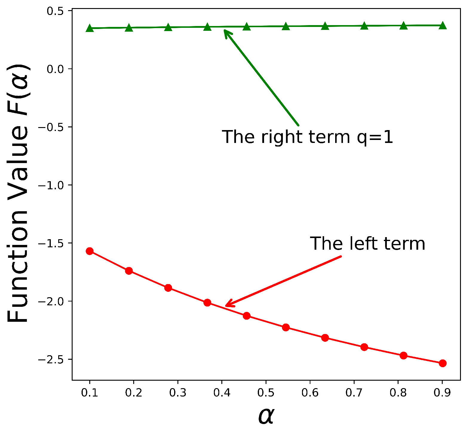
Corollary 5.

When $\sigma \left(x\right)=x,\rho =1$ in Theorem 11, Du and Peng [31] obtain Hermite–Hadamard type inequalities via multiplicative Riemann–Liouville fractional integrals.

Remark 9.

When we take $\sigma \left(x\right)=x$, $\alpha =1$, $\rho =1$ in Theorem 11, it yields the following inequality

$$\begin{array}{cc}\hfill \left|{}_{*}\zeta _f({\mu }_1,{\mu }_2)\right|& ⩽{\left[{\left(f^{*}\left({\mu }_1\right)f^{*}\left({\mu }_2\right)\right)}^{{\left({\displaystyle \frac{1}{2}}\right)}^{{\displaystyle \frac{1}{q}}}}{\left[\begin{array}{c}{f}^{*}\left({\displaystyle \frac{3{\mu }_1+{\mu }_2}{4}}\right)\\ f^{*}\left({\displaystyle \frac{{\mu }_1+3{\mu }_2}{4}}\right)\end{array}\right]}^2{f}^{*}{\left({\displaystyle \frac{{\mu }_1+{\mu }_2}{2}}\right)}^{2^{1-{\displaystyle \frac{1}{q}}}}\right]}^{{\displaystyle \frac{({\mu }_2-{\mu }_1)}{32}}{\left({\displaystyle \frac{2}{3}}\right)}^{{\displaystyle \frac{1}{q}}}},\hfill \end{array}$$

which is presented by Du and Peng in [31].

Example 5.

Let $f\left(t\right)=exp\left\{t^2\right\}$, $t\in (0,\infty )$, the function ${(ln{f}^{*}\left(t\right))}^q={\left(2t\right)}^q$ is convex with $q⩾1$. Thus, all the requirements of Theorem 11 are met. If letting $\rho =1$, ${\mu }_1=1$, ${\mu }_2=2$ and taking $\sigma \left(t\right)=t$ for all $0<\alpha <1$, then, we can obtain the left-hand side of the inequality stated in Theorem 11:

$$\begin{array}{c}exp\left\{{\displaystyle \frac{37}{16}}-\left(\alpha 4^{\alpha -1}\left[\begin{array}{c}{\int }_1^{{\displaystyle \frac{5}{4}}}{(s-1)}^{\alpha -1}{s}^2\mathrm{d}s+{\int }_{{\displaystyle \frac{5}{4}}}^{{\displaystyle \frac{3}{2}}}{\left(s-{\displaystyle \frac{5}{4}}\right)}^{\alpha -1}{s}^2\mathrm{d}s\hfill \\ +{\int }_{{\displaystyle \frac{3}{2}}}^{{\displaystyle \frac{7}{4}}}{\left(s-{\displaystyle \frac{3}{2}}\right)}^{\alpha -1}{s}^2\mathrm{d}s+{\int }_{{\displaystyle \frac{7}{4}}}^2{\left(s-{\displaystyle \frac{7}{4}}\right)}^{\alpha -1}{s}^2\mathrm{d}s\hfill \end{array}\right]\right)\right\}\hfill \\ =exp\left\{{\displaystyle \frac{-252{\alpha }^2-575\alpha -172}{64(\alpha +1)(\alpha +2)}}\right\},\hfill \end{array}$$

and the right portion is equivalent to

$$\begin{array}{c}{\left[\begin{array}{c}{\left(f^{*}\left({\mu }_1\right)\right)}^{{\left({\displaystyle \frac{1}{\alpha +1}}\right)}^{{\displaystyle \frac{1}{q}}}}{f}^{*}{\left({\mu }_2\right)}^{\alpha {\left({\displaystyle \frac{1}{2}}\right)}^{{\displaystyle \frac{1}{q}}}}{f}^{*}{\left({\displaystyle \frac{3{\mu }_1+{\mu }_2}{4}}\right)}^{\left(1+\alpha {\left({\displaystyle \frac{1}{2}}\right)}^{{\displaystyle \frac{1}{q}}}{\left({\displaystyle \frac{\alpha +3}{\alpha +1}}\right)}^{{\displaystyle \frac{1}{q}}}\right)}\hfill \\ f^{*}{\left({\displaystyle \frac{{\mu }_1+{\mu }_2}{2}}\right)}^{\left({\left({\displaystyle \frac{1}{\alpha +1}}\right)}^{{\displaystyle \frac{1}{q}}}+\alpha {\left({\displaystyle \frac{1}{2}}\right)}^{{\displaystyle \frac{1}{q}}}\right)}{f}^{*}{\left({\displaystyle \frac{{\mu }_1+3{\mu }_2}{4}}\right)}^{\left(1+\alpha {\left({\displaystyle \frac{1}{2}}\right)}^{{\displaystyle \frac{1}{q}}}{\left({\displaystyle \frac{\alpha +3}{\alpha +1}}\right)}^{{\displaystyle \frac{1}{q}}}\right)}\hfill \end{array}\right]}^{{\displaystyle \frac{1}{16}}{\left({\displaystyle \frac{1}{\alpha +1}}\right)}^{1-{\displaystyle \frac{1}{q}}}{\left({\displaystyle \frac{1}{\alpha +2}}\right)}^{{\displaystyle \frac{1}{q}}}}\hfill \\ =exp\left\{{\displaystyle \frac{1}{16}}{\left({\displaystyle \frac{1}{\alpha +1}}\right)}^{1-{\displaystyle \frac{1}{q}}}{\left({\displaystyle \frac{1}{\alpha +2}}\right)}^{{\displaystyle \frac{1}{q}}}\left(5{\left({\displaystyle \frac{1}{\alpha +1}}\right)}^{{\displaystyle \frac{1}{q}}}+7\alpha {\left({\displaystyle \frac{1}{2}}\right)}^{{\displaystyle \frac{1}{q}}}+6\alpha {\left({\displaystyle \frac{\alpha +3}{2\alpha +2}}\right)}^{{\displaystyle \frac{1}{q}}}+6\right)\right\}.\hfill \end{array}$$

From the above result, the following inequality can be further established:

$$\begin{array}{c}{\displaystyle \frac{1}{16}}{\left({\displaystyle \frac{1}{\alpha +1}}\right)}^{1-{\displaystyle \frac{1}{q}}}{\left({\displaystyle \frac{1}{\alpha +2}}\right)}^{{\displaystyle \frac{1}{q}}}\hfill \\ \times \left(5{\left({\displaystyle \frac{1}{\alpha +1}}\right)}^{{\displaystyle \frac{1}{q}}}+7\alpha {\left({\displaystyle \frac{1}{2}}\right)}^{{\displaystyle \frac{1}{q}}}+6\alpha {\left({\displaystyle \frac{\alpha +3}{2\alpha +2}}\right)}^{{\displaystyle \frac{1}{q}}}+6\right)\hfill \\ ⩾{\displaystyle \frac{-252{\alpha }^2-575\alpha -172}{64(\alpha +1)(\alpha +2)}}.\hfill \end{array}$$

(17)

By employing numerical estimation and graphical visualization techniques, the results presented in

Table 1. Numerical estimations of (17).

Values $\mathit{\alpha }$	Values of the Left Term	Values of the Right Term
		$\mathit{q}=\mathbf{1}$	$\mathit{q}=\mathbf{5}$
0.1	−1.569399	0.349432	0.606972
0.2	−1.758286	0.354167	0.614122
0.3	−1.918792	0.358173	0.620243
0.4	−2.056920	0.361607	0.625546
0.5	−2.177083	0.364583	0.630188
0.6	−2.282602	0.367187	0.634287
0.7	−2.376021	0.369485	0.637934
0.8	−2.459325	0.371528	0.641202
0.9	−2.534086	0.373355	0.644148

, Figure 8 and Figure 9 demonstrate notable disparities between the left- and right-hand sides of the inequality. Specifically, the left-hand term remains negative and exhibits a continuous decline as $\alpha$ increases, indicating a monotonic downward trend. In contrast, the right-hand term increases with $\alpha$, showing an opposing trend that suggests the possibility of equilibrium under certain parameter conditions. Furthermore, as the parameter q increases, the right-hand term consistently remains positive and continues to grow. These numerical findings are in strong agreement with the theoretical predictions outlined in Theorem 11, thereby reinforcing the validity of the proposed inequality.

Remark 10.

Considering the estimation of bound on the multiplicative right-sided fractional integrals defined as

$$\begin{array}{cc}\hfill {}_f\zeta _{*}(\alpha ,\rho ,\sigma ;{\mu }_1,{\mu }_2)& :={\displaystyle \frac{{\left[f\left({\mu }_1\right)f\left({\mu }_2\right)f\left(\frac{{\mu }_1+{\mu }_2}{2}\right)\right]}^{\frac{1}{4}}}{{\left[\begin{array}{c}{}_{{\mu }_1}I_{*}^{\alpha ,\sigma ,\rho }f\left(\frac{3{\mu }_1+{\mu }_2}{4}\right){·}_{{\sigma }^{-1}\left(\frac{3{\mu }_1+{\mu }_2}{4}\right)}{I}_{*}^{\alpha ,\sigma ,\rho }f\left(\frac{{\mu }_1+{\mu }_2}{2}\right)·\\ {}_{{\sigma }^{-1}\left(\frac{{\mu }_1+{\mu }_2}{2}\right)}I_{*}^{\alpha ,\sigma ,\rho }f\left(\frac{{\mu }_1+3{\mu }_2}{4}\right){·}_{{\sigma }^{-1}\left(\frac{{\mu }_1+3{\mu }_2}{4}\right)}{I}_{*}^{\alpha ,\sigma ,\rho }f\left({\mu }_2\right)\end{array}\right]}^{\frac{4^{\alpha -1}{\rho }^{\alpha }\Gamma \left(\alpha \right)}{{({\mu }_2-{\mu }_1)}^{\alpha }{\gamma }_{\lambda }(\alpha ,1)}}}}.\hfill \end{array}$$

By making use of Remark 10, we can obtain similar results, which will be omitted here.

7. Conclusions

This study investigates multiplicative $\sigma$-convex functions and their interactions with multiplicative generalized proportional $\sigma$-Riemann–Liouville fractional integrals, where $\sigma$ denotes a strictly monotonic and continuous function. Within this framework, we systematically establish Hermite–Hadamard-type inequalities, rigorously validating their analytical soundness and operational domain.

To substantiate the theoretical results, several illustrative examples are provided, demonstrating their practical relevance and applicability. By flexibly adjusting the monotonic function $\sigma$, fine-tuning the proportionality parameter $\rho$, and appropriately selecting the fractional order $\alpha$, we explore the proposed mathematical constructs from multiple perspectives. This parametric flexibility yields a wide range of meaningful and insightful outcomes.

However, due to the exponential kernel structure inherent in the multiplicative fractional integral, the associated analytical expressions become relatively intricate. As such, this paper does not yet include more refined estimations of the function median in the derived Hermite–Hadamard inequalities.

Despite this limitation, the study offers important insights for the continued development of integral inequalities in the setting of multiplicative calculus, particularly those involving multiplicative fractional operators. The methodologies and findings presented herein are expected to foster further research in this direction. As a natural extension, we propose the exploration of broader classes of multiplicative fractional inequalities and their potential applications.

References

1. Nail, B.; Atoussi, M.A.; Saadi, S.; Tibermacine, I.E.; Napoli, C. Real-time synchronisation of multiple fractional-order chaotic systems: An application study in secure communication. Fractal Fract. 2024, 8, 104. [Google Scholar] [CrossRef]
2. Jayaraj, A.P.; Gounder, K.N.; Rajagopal, J. Optimizing signal smoothing using HERS algorithm and time fractional diffusion equation. Expert Syst. Appl. 2024, 238, 122250. [Google Scholar] [CrossRef]
3. Joshi, H.; Yavuz, M.; Townley, S.; Jha, B.K. Stability analysis of a non-singular fractional-order covid-19 model with nonlinear incidence and treatment rate. Phys. Scr. 2023, 98, 045216. [Google Scholar] [CrossRef]
4. Mubeen, S.; Habibullah, G.M. k-Fractional integrals and application. Int. J. Contemp. Math. Sci. 2012, 7, 89–94. [Google Scholar]
5. Sarikaya, M.Z.; Dahmani, Z.; Kiris, M.E.; Ahmad, F. (k, s)-Riemann–Liouville fractional integral and applications. Hacet. J. Math. Stat. 2016, 45, 77–89. [Google Scholar] [CrossRef]
6. Samraiz, M.; Umer, M.; Kashuri, A.; Abdeljawad, T.; Iqbal, S.; Mlaiki, N. On weighted (k, s)-Riemann–Liouville fractional operators and solution of fractional kinetic equation. Fractal Fract. 2021, 5, 118. [Google Scholar] [CrossRef]
7. Jarad, F.; Abdeljawad, T.; Shah, K. On the weighted fractional operators of a function with respect to another function. Fractals 2020, 28, 2040011. [Google Scholar] [CrossRef]
8. Samraiz, M.; Umer, M.; Abdeljawad, T.; Naheed, S.; Rahman, G.; Shah, K. On Riemann-type weighted fractional operators and solutions to cauchy problems. Comp. Model. Eng. 2023, 136, 024029. [Google Scholar] [CrossRef]
9. Khalil, R.; Al Horani, M.; Yousef, A.; Sababheh, M. A new definition of fractional derivative. J. Comput. Appl. Math. 2014, 264, 65–70. [Google Scholar] [CrossRef]
10. Anderson, D.R.; Ulness, D.J. Newly defined Conformable derivatives. Adv. Dyn. Syst. Appl. 2015, 10, 109–137. [Google Scholar]
11. Jarad, F.; Abdeljawad, T.; Alzabut, J. Generalized fractional derivatives generated by a class of local proportional derivatives. Eur. Phys. J. Spec. Top. 2018, 226, 3457–3471. [Google Scholar] [CrossRef]
12. Rashid, S.; Jarad, F.; Noor, M.A.; Kalsoom, H.; Chu, Y.M. Inequalities by means of generalized proportional fractional integral operators with respect to another function. Mathematics 2019, 7, 1225. [Google Scholar] [CrossRef]
13. Jarad, F.; Alqudah, M.A.; Abdeljawad, T. On more general forms of proportional fractional operators. Open Math. 2020, 18, 167–176. [Google Scholar] [CrossRef]
14. Sarikaya, M.Z.; Set, E.; Yaldiz, H.; Başak, N. Hermite–Hadamard’s inequalities for fractional integrals and related fractional inequalities. Math. Comput. Model. 2013, 57, 2403–2407. [Google Scholar] [CrossRef]
15. Vivas-Cortez, M.; Awan, M.U.; Javed, M.Z.; Kashuri, A.; Noor, M.A.; Noor, K.I. Some new generalized κ-fractional Hermite–Hadamard–Mercer type integral inequalities and their applications. AIMS Math. 2021, 7, 3203–3220. [Google Scholar] [CrossRef]
16. Zafar, F.; Mehmood, S.; Asiri, A. Weighted Hermite–Hadamard inequalities for r-times differentiable preinvex functions for k-fractional integrals. Demonstr. Math. 2023, 56, 20220254. [Google Scholar] [CrossRef]
17. Chen, J.; Luo, C. Certain generalized Riemann–Liouville fractional integrals inequalities based on exponentially (h, m)-preinvexity. J. Math. Anal. Appl. 2024, 530, 127731. [Google Scholar] [CrossRef]
18. Saleh, W.; Lakhdari, A.; Kiliçman, A.; Frioui, A.; Meftah, B. Some new fractional Hermite–Hadamard type inequalities for functions with co-ordinated extended (s, m)-prequasiinvex mixed partial derivatives. Alex. Eng. J. 2023, 72, 261–267. [Google Scholar] [CrossRef]
19. Mumcu, İ.; Set, E.; Akdemir, A.O.; Jarad, F. New extensions of Hermite–Hadamard inequalities via generalized proportional fractional integral. Numer. Methods Partial. Differ. Equ. 2021, 40, 22767. [Google Scholar] [CrossRef]
20. Grossman, M.; Katz, R. Non-Newtonian Calculus: A Self-Contained, Elementary Exposition of the Authors’ Investigations; Lee Press: Pigeon Cove, MA, USA, 1972. [Google Scholar]
21. Özcan, S. Some integral inequalities of Hermite–Hadamard type for multiplicatively preinvex functions. AIMS Math. 2020, 5, 1505–1518. [Google Scholar] [CrossRef]
22. Özcan, S. Hermite–Hadamard type inequalities for multiplicatively p-convex functions. J. Inequal. Appl. 2023, 2023, 121. [Google Scholar] [CrossRef]
23. Özcan, S.; Butt, S.I. Hermite–Hadamard type inequalities for multiplicatively harmonic convex functions. J. Inequal. Appl. 2023, 2023, 120. [Google Scholar] [CrossRef]
24. Özcan, S. Hermite–Hadamard type inequalities for exponential type multiplicatively convex functions. Filomat 2023, 37, 9777–9789. [Google Scholar] [CrossRef]
25. Xie, J.; Ali, M.A.; Thanin, S. Some new midpoint and trapezoidal type inequalities in multiplicative calculus with applications. Filomat 2023, 37, 6665–6675. [Google Scholar] [CrossRef]
26. Meftah, B.; Lakhdari, A.; Saleh, W.; Benchettah, D.C. Companion of Ostrowski inequality for multiplicatively convex functions. Sahand Commun. Math. Anal. 2024, 21, 289–304. [Google Scholar] [CrossRef]
27. Meftah, B.; Lakhdari, A. Dual Simpson type inequalities for multiplicatively convex functions. Filomat 2023, 37, 7673–7683. [Google Scholar] [CrossRef]
28. Chasreechai, S.; Ali, M.A.; Naowarat, S.; Sitthiwirattham, T.; Nonlaopon, K. On some Simpson’s and Newton’s type of inequalities in multiplicative calculus with applications. AIMS Math. 2023, 8, 3885–3896. [Google Scholar] [CrossRef]
29. Budak, H.; Özçelik, K. On Hermite–Hadamard type inequalities for multiplicative fractional integrals. Miskolc Math. Notes 2020, 21, 91–98. [Google Scholar] [CrossRef]
30. Kashuri, A.; Sahoo, S.K.; Aljuaid, M.; Tariq, M.; Sen, M.D.L. Some new Hermite–Hadamard type inequalities pertaining to generalized multiplicative fractional integrals. Symmetry 2023, 15, 868. [Google Scholar] [CrossRef]
31. Du, T.; Peng, Y. Hermite–Hadamard type inequalities for multiplicative Riemann–Liouville fractional integrals. J. Comput. Appl. Math. 2024, 440, 115582. [Google Scholar] [CrossRef]
32. Zhang, L.; Peng, Y.; Du, T. On multiplicative Hermite–Hadamard and Newton-type inequalities for multiplicatively (P, m)-convex functions. J. Math. Anal. Appl. 2024, 534, 128117. [Google Scholar] [CrossRef]
33. Peng, Y.; Özcan, S.; Du, T. Symmetrical Hermite–Hadamard type inequalities stemming from multiplicative fractional integrals. Chaos Solitons Fractals 2024, 183, 114960. [Google Scholar] [CrossRef]
34. Zhou, Z.; Du, T. Analytical properties and related inequalities derived from multiplicative Hadamard k-fractional integrals. Chaos Solitons Fractals 2024, 189, 115715. [Google Scholar] [CrossRef]
35. Wu, S.; Awan, M.U.; Noor, M.A.; Noor, K.I.; Iftikhar, S. On a new class of convex functions and integral inequalities. J. Inequal. Appl. 2019, 2019, 131. [Google Scholar] [CrossRef]
36. Bin-Mohsin, B.; Javed, M.Z.; Awan, M.U.; Kashuri, A. On some new AB-fractional inclusion relations. Fractal Fract. 2023, 7, 725. [Google Scholar] [CrossRef]
37. Javed, M.Z.; Awan, M.U.; Ciurdariu, L.; Dragomir, S.S.; Almalki, Y. On extended class of totally ordered interval-valued convex stochastic processes and applications. Fractal Fract. 2024, 8, 577. [Google Scholar] [CrossRef]
38. Bin-Mohsin, B.; Javed, M.Z.; Awan, M.U.; Meftah, B.; Kashuri, A. Fractional reverse inequalities involving generic interval-valued convex functions and applications. Fractal Fract. 2024, 8, 587. [Google Scholar] [CrossRef]
39. Sahoo, S.K.; Tariq, M.; Ahmad, H.; Kodamasingh, B.; Shaikh, A.A.; Botmart, T.; El-Shorbagy, M.A. Some novel fractional integral inequalities over a new class of generalized convex functions. Fractal Fract. 2022, 6, 42. [Google Scholar] [CrossRef]
40. Bashirov, A.E.; Kurpınar, E.M.; Özyapıcı, A. Multiplicative calculus and its applications. J. Math. Anal. Appl. 2008, 337, 36–48. [Google Scholar] [CrossRef]
41. Ali, M.A.; Budak, H.; Sarikaya, M.Z.; Zhang, Z. Ostrowski and Simpson type inequalities for multiplicative integrals. Proyecciones 2021, 40, 743–763. [Google Scholar] [CrossRef]
42. Niculescu, C.P. Convexity according to the geometric mean. Math. Inequal. Appl. 2000, 3, 155–167. [Google Scholar] [CrossRef]
43. Abdeljawad, T.; Grossman, M. On geometric fractional calculus. J. Semigroup Theory Appl. 2016, 2016, 2. [Google Scholar]
44. Kacar, E.; Kacar, Z.; Yildirim, H. Integral inequalities for Riemann–Liouville fractional integrals of a function with respect to another function. Iranian J. Math. Sci. Inform. 2018, 13, 1–13. [Google Scholar] [CrossRef]
45. Zhou, S.-S.; Rashid, S.; Rauf, A.; Jarad, F.; Hamed, Y.S.; Abualnaja, K.M. Efficient computations for weighted generalized proportional fractional operators with respect to a monotone function. AIMS Math. 2021, 6, 8001–8029. [Google Scholar] [CrossRef]
46. Mohammed, P.O.; Sarikaya, M.Z.; Baleanu, D. On the generalized Hermite–Hadamard inequalities via the tempered fractional integrals. Symmetry 2020, 12, 595. [Google Scholar] [CrossRef]
Figure 1. Curves of I 0.01 α , σ * ρ f ( t ) for different α .
Symmetry 17 00702 g001
Figure 2. Curves of I 0.01 α , σ * ρ f ( t ) for different ρ .
Symmetry 17 00702 g002
Figure 3. Curves of I 0.01 α , σ * ρ f ( t ) for different σ .
Symmetry 17 00702 g003
Figure 4. Visual for α [ 0.1 , 0.99 ] , ρ [ 0.1 , 0.99 ] .
Symmetry 17 00702 g004
Figure 5. Visual for α [ 0.1 , 0.99 ] , ρ = 1 .
Symmetry 17 00702 g005
Figure 6. Visual for ρ [ 0.1 , 0.99 ] , α = 1 .
Symmetry 17 00702 g006
Figure 7. Visual for α [ 0.1 , 0.99 ] , ρ [ 0.1 , 0.99 ] .
Symmetry 17 00702 g007
Figure 8. The visual of (17), when q = 1 .
Symmetry 17 00702 g008
Figure 9. The visual of (17), when q = 5 .
Symmetry 17 00702 g009