Abstract
A significant challenge in probabilistic seismic demand analysis lies in selecting appropriate intensity measures and investigating their relationships with demand parameters to ensure accurate seismic fragility predictions. A single ground motion intensity measure is insufficient to capture the complex characteristics of ground motion, leading researchers to focus on compound intensity measures. It is essential to investigate the selection of ground motion features and the number of features included in the construction of compound intensity measures, as these measures cannot comprise an unlimited set of ground motion features. This study focused on machine learning feature selection methods to select ground motion features for compound intensity measures, utilizing mutual information for feature selection. Considering the symmetry and asymmetry requirements of this process, optimized features were selected. Based on the selected features, the compound ground motion intensity measure was constructed to evaluate structural seismic fragility. The compound ground motion intensity measure was evaluated against scalar intensity measure in terms of correlation, efficiency, practicality, proficiency, and sufficiency. A comprehensive comparative analysis demonstrates the applicability of the compound intensity measure. The study’s findings support fragility analysis and performance evaluation using compound intensity measures. The corresponding results can be applied in the risk analysis aspect of performance-based earthquake engineering.
1. Introduction
Asymmetric models break through the limitations of traditional symmetric models (e.g., normal distributions) on symmetry assumptions by introducing asymmetric structures (e.g., bias, tail differences, or parameter designs), enabling them to more flexibly describe biased data, extreme events, and tail risks prevalent in the real world. As an important representative of asymmetric models, the lognormal distribution is widely used in the fields of reliability analysis, risk assessment, and signal processing.
Performance-based earthquake engineering (PBEE) is primarily used to assist in the completion of seismic design and performance evaluation tasks pertaining to structure. In the PBEE framework, precise earthquake damage estimation and prediction are essential for the seismic performance of structures [1]. Seismic fragility analysis serves as the core step in PBEE. It mainly estimates the conditional probability that structural damage reaches or exceeds at a certain failure state under given ground motion intensity conditions [2,3]. The probabilistic seismic demand model (PSDM) effectively characterizes the relationship between ground motion intensity measures (IMs) and seismic engineering demand parameters (EDPs) within the framework of seismic fragility analysis.
The appropriate intensity measure (IM) shows a good correlation with EDPs to establish the relationship between IMs and EDPs. The accuracy of structural damage prediction with high confidence in the PSDM and seismic fragility analysis is improved by a suitable IM. An important aspect of the PSDM is the selection of a suitable IM to ensure accurate prediction of EDPs [4,5]. Hence, choosing preferable IMs for ground motions (GMs) has received widespread attention.
To determine optimal ground motion IMs, a large number of prior studies have been conducted in recent years about correlations between EDPs (obtained with nonlinear structural analysis) and IMs [6,7,8]. Numerous IMs have been proposed by researchers. These IMs can be classified into structure-specific and non-specific ones. Structure-related IMs uses structure-specific parameters to capture ground motion characteristics, while non-structure-specific IMs are obtained through direct time history recording [9], such as Peak Ground Acceleration (PGA), Peak Ground Velocity (PGV), and so on. PGA and PGV are commonly employed as available IMs owing to their ease of use and accessibility for seismic design and structural damage estimation [10]. Yet, PGA is not always the optimal ground motion IM, particularly in medium- and long-period structures, which may not adequately represent structural seismic performance [11]. In general, spectral acceleration at the fundamental period is more efficient than PGA, since it can better capture the features of ground motion for evaluating structural responses [12].
However, some studies have shown that may not be an especially effective or appropriate predictor in some situations, such as near-fault ground motions or long-period structures [13]. Eads et al. [14] investigated the use of the geometric mean of spectral acceleration over a certain period interval () as an intensity measure (IM) to estimate structural collapse risk. It was shown that computed using an appropriate period range usually obtains more efficient and stable risk estimation results compared to . Similarly, Adam et al. [15] revealed that dispersion is minimized or nearly minimized when using to estimate collapse risk.
Only considering a single ground motion IM may not encapsulate sufficient information of ground motions due to the complexity of earthquake ground motions, leading to biased estimation [16,17]. In order to more comprehensively capture the characteristics of ground motion, researchers have developed vector IMs. Single-parameter IMs are referred to as scaler IMs, whereas vector IMs are IMs with several parameters that represent various characteristics of ground motions [18,19].
Previous research has demonstrated that vector IM can decrease uncertainty in probabilistic seismic demand analysis and increase the efficiency of structure response estimation [20,21]. Kohrangi et al. [22] employed vector and scalar IMs in the response assessment and the selection of seismic records using conditional spectrum selection, concluding that the risk estimation and fragility analysis for vector IM is more accurate. Bojórquez et al. [23] examined the seismic fragility of steel frame structures using vector parameters. The outcome demonstrated that the vector value IM-based spectral shape is the most representative parameter in the estimation of response and demand. More ground motion features are captured and structural response is more precisely estimated by vector-valued IMs with two parameters than by scalar-valued IMs.
Although researchers have proposed vector IMs to facilitate more accurate structural demand analysis, there are still a lot of works to propose more novel IMs to capture more features of ground motion within the seismic performance assessment framework [24]. In recent years, researchers have developed a large number of compound IMs to comprehensively reflect more ground motion features, some of which incorporate the contribution of higher modes [13,17]. Pinzón et al. [25] proposed a new IM based on PGV and significant duration (between 5 and 95% of the Arias intensity) as variables, which are highly correlated with the maximum inter-story drift ratio (MIDR) in steel frame buildings. Furthermore, Liu et al. [26] proposed a compound IM by using the typical correlation analysis CCA method to evaluate the structural performance. Liu et al. [27] developed a compound IM for assessing structural damage by extracting the main factors and linearly combining them using the exploratory factor analysis (EFA) approach. Liu et al. [28] developed a compound IM to perform probabilistic seismic demand analysis by establishing a multiple regression model employing the partial least squares method. Similarly, Sun [29] et al. and Chen et al. [30] also developed a compound IM using the least squares approach to evaluate the seismic performance of cross-fault hydraulic tunnels and obtain the severest design ground motion of underground buildings, respectively. Wang et al. [31] applied a machine learning approach to establish a probabilistic demand model considering multiple IMs for fragility assessment of nuclear power plants. In summary, these investigations collectively demonstrate that the compound IM effectively integrates various aspects of ground motion features, exhibits a strong correlation with EDPs, and is well suited for fragility analysis.
It is essential to investigate the selection of ground motion features and determine the appropriate number of features to be included in the construction of a compound intensity measure, as the measure cannot indefinitely incorporate ground motion features. In this paper, we refer to the feature selection method of machine learning to select ground motion feature parameters for compound IMs. Firstly, a structural model is established, the ground motion record set is chosen as the input, and a series of nonlinear time history analyses are carried out to obtain the structural response. Then, feature selection using the mutual information method is performed to construct a compound IM of ground motion for evaluating structural performance. Finally, the compound IM of ground motion is compared and evaluated from the perspective of efficiency, proficiency, and adequacy. The common single IM and the proposed compound IM are compared and analyzed in many aspects to further reveal the applicability of the compound IM. The results of this study contribute to seismic fragility analysis and performance evaluation based on compound IMs.
2. Compound IM Construction of Ground Motion
2.1. Candidate IMs
Optimal intensity measures should capture ground motion features and have a strong correlation with structural damage. Therefore, the selection of optimal intensity measures is crucial to reduce the estimation bias of EDPs and improve seismic fragility analysis and performance evaluation. Each single IM provides a part of the ground motion features. Structural seismic damage can be precisely and efficiently assessed by combining a number of useful features of ground motions. In order to make the compound IM capture the features of ground motion as comprehensively as possible, it is necessary to propose sufficient ground motion intensity measures. A considerable number of intensity measures have been proposed, which can be used as candidate parameters for the compound IM. According to the features of ground motion, these candidate intensity measures can be classified into four categories: duration, spectrum, amplitude, and integral type. Integration-type IMs are time integrations over one or more of the preceding intensity measure categories, such as CAV MIV, etc. Information about these candidate intensity measures is shown in Table 1.

Table 1.
Candidate IMs in the present study.
2.2. Mutual Information Theory
The ground motion information provided by different ground motion IMs may overlap, so it is necessary to select available IMs to construct the compound IM. Feature selection aims to select features containing rich target information from an extensive array of features to address regression and classification problems. Generally, feature selection algorithms can be typically classified into three categories: filter model, wrapper model, and embedding model [43,44,45]. The wrapper model incurs significant computational expenses and poses a danger of overfitting. The embedded model selects features in the training process of the learning machine. And it is difficult to construct an objective function optimization model. Compared to the wrapper model and the embedded model, the filter model exhibits superior generalization ability and reduced computational cost [44,46]. Numerous indicators are employed in filtering procedures, including consistency, distance, and mutual information. Methods based on information theory are widely applied in filter models, because information theory can effectively evaluate linear and nonlinear correlations between variables [47,48]. In this paper, a filter model based on information theory is employed for feature selection.
This section presents fundamental concepts of information theory. Entropy is a fundamental term in the information theory utilized to evaluate the uncertainty associated with random data. Designate X, Y, and Z as random variables. The definition of entropy is shown in Equation (1).
where is the probability distribution of variable x, and is the entropy of variable x.
Conditional entropy quantifies the uncertainty of one variable given the state of another variable. Given a random variable X, the conditional entropy of Y given the X condition is shown in Equation (2).
where denotes conditional entropy, is a joint probability distribution function of random variables X and Y, and is the conditional probability distribution function of the random variable Y given X.
Mutual information can be employed to measure the shared information of two variables. The specific definition of mutual information is shown in Equation (3).
where is the mutual information of X and Y.
Supplementing the information of one variable may reduce the uncertainty of the other. Therefore, mutual information can indicate the independence and correlation between two variables. Mutual information satisfies symmetry, i.e., I(X; Y) = I(Y; X), indicating that MI is direction-independent between X and Y. Whether measured from X to Y or vice versa, the value remains identical.
Feature selection aims to identify features with the highest predictive value for a target variable, such as a classification label or regression output. Although mutual information is inherently symmetric, feature selection imposes an asymmetric demand. Specifically, feature selection focuses on the amount of information that the feature provides about the target variable, rather than the reverse. While high mutual information may reflect strong associations between variables, feature selection requires a goal-oriented asymmetry to identify the most relevant features. In high-dimensional data, redundant features, those with high mutual information among themselves but low relevance to the target variable, must be excluded. In high-dimensional datasets, it is essential to exclude redundant features—those exhibiting high mutual information among themselves but demonstrating low relevance to the target variable. A distinction must be made between the symmetry among features and the asymmetry of features concerning the target variable.
When , it reflects the correlation between the two variables. The relationship between mutual information and entropy is shown in Equation (4).
Conditional mutual information represents the amount of information between X and Y, when Z is given. The conditional mutual information is represented by Equation (5).
Joint mutual information is also an important concept in information theory. Joint mutual information denotes the mutual information between (X, Y) and Z.
The interaction information represents the mutual information among three random variables, which is frequently utilized to indicate feature redundancy information in feature selection. The relationship between interactive information and conditional mutual information is illustrated in Formula (7).
Interaction information has a relationship with joint mutual information and mutual information , , as expressed in Equation (8).
The random variable Z is set as the dependent variable, and the random variables X and Y are independent variables, which are the features to be selected. According to Equation (8), it can be found that when , i.e., , the sum of information provided by random variables X and Y alone exceeds the information provided by the combination of the two. When , the information provided by the combination of random variables X and Y exceeds the cumulative information provided by each variable independently. This shows that the combination of random variables X and Y provides information that cannot be provided when the two are alone. This means that when , the selected feature can provide more information.
Minimum Redundancy Maximum Relevance (mRMR) is a feature selection technique based on mutual information, designed to identify a subset of features that exhibit a high correlation with the target variable while maintaining low redundancy among themselves. The mRMR achieves this by simultaneously considering maximum correlation and minimum redundancy. “The calculation formula of mRMR [49] evaluation criteria is as follows”.
The Conditional Infomax Feature Extraction (CIFE) [50] aims to obtain the most informative features. This feature extraction method considers correlation, interactivity, and redundancy indexes at the same time. The calculation formula is as follows:
Gao et al. [51] proposed a feature selection method called the Combination of Feature Relevance (CFR). The definition of CFR is shown as Equation (11).
where represents the candidate feature, is the selected feature, and Y is the dependent variable.
According to the aforementioned concepts related to information theory, the derivation of the CFR can yield Formula (12).
In the process of selecting features, it is essential to evaluate not only the correlation between the features and the dependent variables but also the interrelationship among the selected features and their combined effect on the estimation of the dependent variables. The CFR approach emphasizes the link between the features to be selected and the dependent variable, while ensuring that the inclusion of features enhances the relevance of the overall selection and minimizes redundant information.
2.3. Construction of Compound Ground Motion IM
The compound IM exhibits various ground motion features, and a probabilistic demand model can be developed using multiple IMs. Probabilistic demand models typically employ regression analysis to establish the relationship between IMs and EDPs. In addition to ordinary least squares regression, numerous regression approaches have been proposed for evaluating structural damage, including principal component analysis [52], exploratory factor analysis [27], canonical correlation analysis [26], and partial least squares [28]. This paper initially conducted feature selection using the mutual information method to determine the ground motion IMs. Subsequently, ordinary least squares regression and a partial least squares approach were employed for multiple linear regression to formulate the compound IM and develop the probability demand model. When ordinary least squares regression was utilized, the selected features were assessed for multicollinearity due to the potential linear correlation among various IMs. The candidate features exhibiting a variance inflation factor exceeding 10 were eliminated to avoid the detrimental impact of multicollinearity on regression results.
Figure 1 shows the flow of the feature selection method. The specific method steps are described as follows:
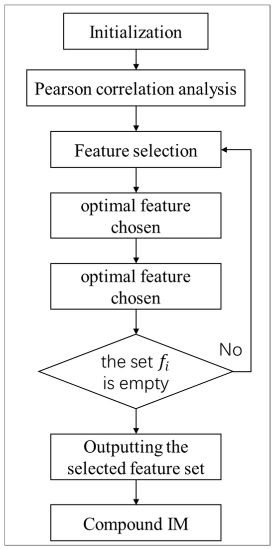
Figure 1.
Flowchart of feature selection method.
First step, initialization: The original feature set of ground motion is obtained as the candidate feature set , and is an empty set.
Step 2, Pearson correlation analysis: Pearson correlation analysis is performed on the features of the original feature set of the alternate features. If the Pearson correlation coefficient between the two feature parameters exceeds 0.85, a strong linear relationship is indicated, potentially resulting in multicollinearity. Pearson correlation analysis is conducted on these features alongside the seismic demand value of the target variable to identify the most pertinent features. If the correlation coefficient of two candidate IMs is higher than 0.85, the feature that is more relevant to the target variable is retained and the other one is excluded. The retained feature is used as the preliminary selection of features.
Step 3, feature selection procedure: The initially selected features serve as the candidate feature set for calculating the mutual information index between each candidate feature and the target variable. The mutual information is computed between the selected features and the candidate features, between the selected features and the target variable Y, and the joint mutual information among the candidate features, selected features, and target variables to derive the mutual information results of the used mRMR, CIFE, or CFR algorithm.
Step 4, optimal feature selection: By computing the mutual information between each candidate feature and the target variable, the features that optimize the mRMR, CIFE, or CFR are chosen for inclusion in feature set S. The chosen features are evaluated for multicollinearity, which will eliminate any feature set S that could result in significant multicollinearity issues.
Step 5, iteration: The preceding two steps are repeated until the quantity of selected features attains the specified target or all alternative features are evaluated and the candidate feature set is exhausted.
Step 6, analysis and comparison: The specified feature set is output and ordinary least squares regression is employed for multiple linear regression analysis. The results are used for comparison to the outcomes of partial least squares regression following Pearson correlation analysis.
A compound IM is ultimately produced and assessed against the evaluation index of a singular parameter to ascertain the ideal parameters.
The compound IM derived from the mutual information method can be expressed according to Equation (11).
By applying logarithms to both sides of the equation, the compound IM can be represented as a log-linear combination of the selected feature parameters with the following expression in Equation (12).
where are regression coefficients, and are selected IMs based on mutual information method.
3. Seismic Record Set and Structural Model
3.1. Selection of Ground Motion Record Set
Ground motion records were selected from the PEER strong ground motion database to establish the ground motion record set and to derive the seismic fragility curve. The earthquake magnitude M and epicentral distance R were constrained to the intervals 5.8 ≤ M ≤ 8 and 10 km ≤ R ≤ 60 km. A total of 1724 pairs of horizontal ground motion records were selected within this range. The ground motion records in one direction were used as training dataset, while those in the other direction were used as test dataset. Figure 2 illustrates the earthquake magnitude and epicentral distance distribution for ground motion records utilized in seismic fragility analysis.
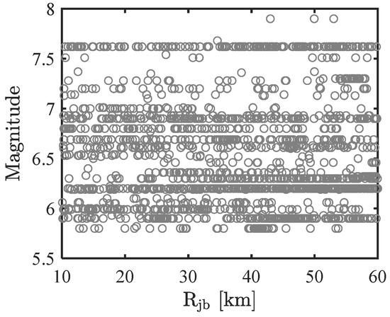
Figure 2.
Scatter plot of magnitude and source to site distance corresponding to the selected ground motion records.
3.2. Structural Model
In this paper, structural models of four reinforced concrete frame structures with different numbers of stories [53] were constructed according to the Chinese seismic design code for nonlinear dynamic analysis. The four constructions consisted of three, five, eight, and ten stories, with the first floor measuring 4.4 m in height and the subsequent stories each measuring 3.3 m. The side span measured 6 m, while the central span measured 2.4 m. The distance between frames in the perpendicular direction was 6.0 m. In this paper, the middle one-bay planar frame was selected as the research object and the structural response was obtained by modeling and analyzing using finite element software OpenSees (version 3.2.2) [54]. The beams and columns of the structure were made of C30 concrete and the longitudinal reinforcement was made of HRB335. The influence of infill walls and slabs was not considered and the beam-column joints were not specially defined, but were treated as solid joints. Using the five-story reinforced concrete frame construction as a case study, Figure 3 shows the dimension information and cross-section reinforcement of the application case. The distinction between the other structures and the five-story structure was in the number of stories, regarding building dimensional specifications.
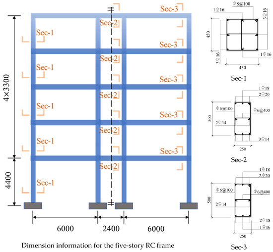
Figure 3.
The dimensional information and section reinforcement of the applied five-story structure (Sec-1 shows the column cross-section reinforcement, and Sec-2 and Sec-3 show the beam cross-section reinforcement for the five-story structure).
4. Feature Parameter Selection
4.1. Pearson Correlation Coefficient
Applying too many features of ground motions directly to regression analysis may lead to model complexity and diminished predictive performance, hence necessitating feature selection. The Pearson correlation coefficient is a prevalent metric for assessing the strength and direction of linear correlations between two continuous variables, commonly utilized in feature selection. The coefficient (designated as R) ranges from −1 to +1: values approaching +1 signify a robust positive correlation (i.e., both variables increase concurrently), whereas values nearing −1 denote a strong negative correlation (i.e., one variable ascends as the other descends). An R value of 0 indicates the absence of a linear correlation between variables.
Given two sets of data and , the Pearson correlation coefficients are calculated as follows:
where and are the ith observation of the input feature variables X and Y, respectively; and are the mean values of X and Y, respectively.
Taking the maximum inter-story drift ratio as the seismic demand parameter, Figure 4 illustrates the Pearson correlation coefficients between candidate seismic ground motion features and the seismic demand parameters of the four structures. The ranking of these coefficients for the three-story structure is extended to other structures. Among positively correlated features, those with coefficients below 0.2 are deemed to indicate a weak correlation. The logarithmic results of Bracketed_Dur (bracketed duration) and Uniform_Dur (uniform duration) exhibit weak linear positive correlations with structural demand variables. If Pearson correlation analysis is employed for feature selection, these features with weak correlations are excluded from the candidate set. A heatmap depicting the associations among the 25 features and structural seismic demand parameters is shown in Figure 5 for future investigation.
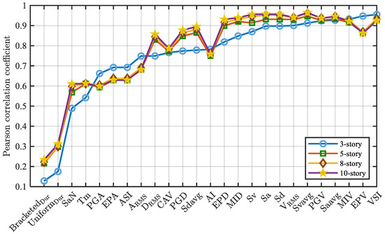
Figure 4.
Analysis of Pearson correlation using logarithmic features.
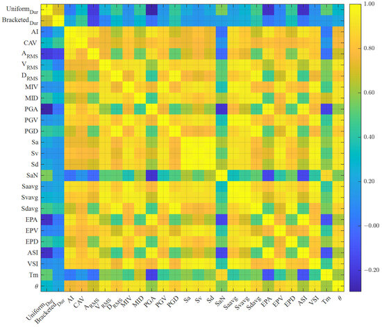
Figure 5.
Pearson correlation heatmap.
Heatmaps can be used to explore the correlation between each of the two parameters for the twenty-five feature parameters and structural seismic demand parameters. In this heatmap, warmer hues indicate higher correlation coefficients, while cooler hues represent diminished values. The Pearson correlation heatmap indicates that the spectral acceleration, velocity, and displacement parameters demonstrate exceptionally high correlations (exceeding 0.96). Additionally, average spectral acceleration (Saavg), average spectral velocity (Svavg), and peak ground velocity (PGV) and velocity spectrum intensity (VSI) show high correlations (exceeding 0.9) with maximum incremental displacement (MIV). Elevated inter-feature correlations suggest substantial linear interactions, potentially resulting in multicollinearity problems. Multicollinearity can lead to unstable regression coefficient estimates, diminished variable significance, and elevated standard errors, thus undermining model interpretability and predictive efficacy.
Consequently, when several candidate features have significant linear correlations, it is advisable to keep only one feature that is strongly correlated with the response variable to reduce the hazards of multicollinearity. In this paper, to balance feature retention and correlation with seismic demand parameters, non-core features with weak associations were identified, and they would be excluded in the analysis of the compound ground motion intensity measure to minimize computational workload and enhance feature selection efficiency.
4.2. Multiple Regression Prediction
After employing the CFR mutual information method for feature selection, subsets of features were determined for four structures based on mutual information indices. Based on the results of each structure’s feature selection, a set of 1724 ground motion records in a certain horizontal direction was selected as the training set to construct a multiple linear regression (MLR) model, while another set of 1724 records served as the testing set to compare regression errors. Figure 6 presents scatter plots of predicted versus observed values in the test sets for three-story, five-story, eight-story, and ten-story structures, with the x-axis indicating actual values and the y-axis representing predicted values. Additionally, Figure 7 displays the R2 results for the MLR model, assessing the predictive accuracy of logarithmic seismic demand parameters.
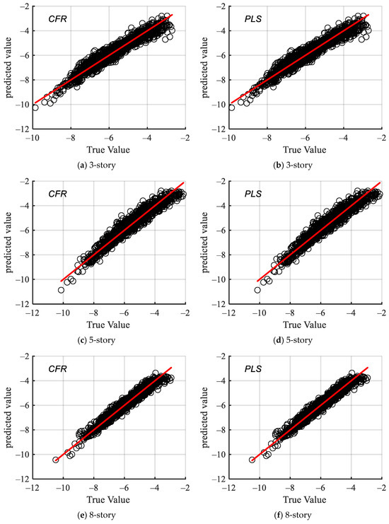
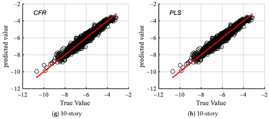
Figure 6.
Scatter of seismic demand distribution graph of 3-story structure for Combination of Feature Relevance (CFR) method and Partial Least Squares (PLS) regression method.
Figure 7.
Comparison of coefficients of determination .
The scatter plot analysis indicates that features selected based on the mutual information criterion enhanced MLR prediction performance, closely approximating the fit of the partial least squares (PLS) regression. To further assess model performance, the coefficient of determination (R2) was employed, a critical statistic in regression analysis that quantifies the proportion of variance in the dependent variable (response variable) explained by the independent variables (predictors). Figure 7 illustrates that both the MLR and PLS models exhibit exceptional data fit, with R2 values surpassing 0.9, signifying the strong explanatory capacity of the predictors. This discovery highlights the efficacy of mutual information-based feature selection for seismic demand parameter analysis and fragility assessment. Ultimately, the optimal feature subset identified via mutual information was adopted to construct the compound ground motion intensity measure.
5. Probabilistic Seismic Fragility Analysis
5.1. Analysis Method
Fragility reflects the conditional probability that the structural damage measure (DM) reaches or exceeds a certain limit state at a specific IM level. Fragility analysis, an important part of PBEE, is employed to quantify the seismic reliability and risk of structures. Probabilistic seismic demand analysis (PSDA) serves fragility analysis by establishing appropriate probabilistic seismic demand models and obtaining the relationship between structural DMs and ground motion IMs.
In this paper, the cloud diagram method is used to model probabilistic seismic demand [55]. This method utilizes unscaled ground motion records to establish a demand model, and the structural probabilistic seismic demand model based on the lognormal distribution assumption is shown in following formula.
where IM denotes the ground motion intensity measure, EDP signifies the seismic engineering demand parameter, edp indicates the seismic demand limit, and represent the median and logarithmic standard deviation of the seismic demand of the structure under the action of the specific ground motion intensity measure, and Φ(·) is the standard normal cumulative distribution function.
The linear regression model of EDP and IM in the logarithmic space is as follows.
where a and b represent the coefficients of linear regression. Traditionally, when using the cloud analysis method, the values of coefficients a and b can be derived using the least squares approach.
Then, can be computed using Equation (16):
where N is the quantity of input ground motion records, and is the ith engineering demand parameter.
5.2. Probabilistic Seismic Demand Model
This paper constructs the compound ground motion intensity measure corresponding to four structures, following the methodology outlined in Section 2.3. Taking the three-story structure as an example, the constructed compound IM is shown in Equation (17).
Selecting a compound IM can enhance the prediction of structural EDPs. In order to further investigate the applicability of the compound IM, probabilistic demand analysis is performed on the nonlinear response results of the three-story structure. According to Equation (17), a linear regression analysis of the compound IM and EDPs is performed to establish a probabilistic demand model. Simultaneously, as a comparison, the probability demand models of other scalar IMs are also established. These scalar IMs include the scalar IMs that constitute the compound IM, as well as other commonly used scalar IMs such as PGA and Sa. The scatter plots and fitted straight lines of the EDP and the corresponding multiple IMs are depicted in Figure 8 and Figure 9. In addition, the regression line equation and the 95% confidence interval are shown in the bottom right of the figure, while the goodness-of-fit value is presented in the top left corner. The goodness-of-fit is a crucial index for evaluating the efficacy of a linear regression model, which measures the degree of fitting of the model to the data. The coefficient of determination serves as the indicator of quality of fit in this context. The coefficient of determination indicates that the fitting quality of derived from the mutual information approach is better than that of the other IMs. Specifically, performs marginally better than the best scalar IM, the VSI, which has the highest fitting performance among all scalar intensity measures.
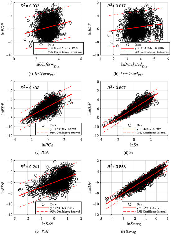
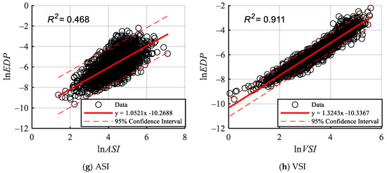
Figure 8.
Seismic demand in the regression coefficient with the different IMs based on the PSDM.
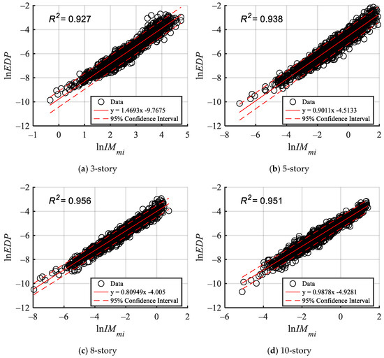
Figure 9.
Seismic demand in the regression coefficient with based on the PSDM.
5.3. Evaluation Criteria
The performance of the IM is evaluated according to a certain criterion to determine the optimal IM for the probabilistic demand model. This paper employs correlation, efficiency, practicality, and proficiency as the evaluation criteria of the IM.
5.3.1. Correlation
Correlation is a significant term in statistics that describes the relationship between the IM and DM. It measures the strength and direction of the linear relationship between variables. Correlation does not denote causation; it merely indicates that there is some connection between the variables. Pearson’s correlation coefficient is a statistical measure that quantifies the correlation between variables. The value range is from −1 to 1. A value closer to 1 indicates a stronger positive correlation, whereas a value closer to 0 signifies a weaker correlation.
The correlation coefficients between each IM and EDP are illustrated in Figure 10. Figure 10 depicts the Pearson correlation coefficients between various IMs (Sa, Savag, VSI, and ) and seismic demand parameters (EDPs) across different structures. For the three-story structure, the Pearson correlation coefficients of Sa, Savag, VSI, and with EDPs all exceed 0.85, with exhibiting the highest correlation. Similarly, in five-story, eight-story, and ten-story structures, the correlation coefficients of Sa, Savag, Svvag, VSI, and with EDPs exceed 0.9, where consistently demonstrates the strongest correlation. Significantly, it has the strongest correlation among all IMs across various structures, highlighting its strong association with EDPs. The primary reason lies in the compound nature of , which encapsulates more effective information relevant to structural demands, therefore forming a robust and durable association with EDP across four distinct structures.
Figure 10.
Correlation of and other scalar parameters with engineering demand parameters (maximum inter-story drift ratio, ; The red dotted line represents the value of ).
5.3.2. Efficiency
Efficiency is a frequently employed criterion for selecting an optimal IM. An efficient IM can decrease variation and dispersion in demand estimations for a given IM value [56]. The standard deviation of structural demand in IM-DM log-linear regression is employed to investigate IM efficiency, which is calculated according to Equation (16). A reduced standard deviation indicates increased effectiveness of the IM.
Figure 11 presents the dispersion parameters of structural engineering demand parameters under seismic excitations for four different structures. The efficacy of Sa, Savag, Svvag, VSI, and other variables is similarly illustrated by correlation analysis. Notably, the standard deviation of is minimal across all IMs for each structure, indicating its optimal efficacy in minimizing the dispersion of structural response estimates. In other words, can significantly diminish the estimation error of structural demand consequences.

Figure 11.
Efficiency of and other scalar parameters (The red dotted line represents the value of ).
5.3.3. Practicality
The practicality of a seismic intensity measure (IM) is measured by its impact on engineering demand parameters (EDPs), with increased practicality implying greater sensitivity of EDPs to variations in the IM. This is typically denoted by the slope of the logarithmic linear regression model. As illustrated in Figure 12, the slope of the logarithmic-linear regression for in three-story structures is the largest among all IMs, indicating its pronounced influence on EDPs. Although the practicality of decreases in taller structures, it still outperforms several scalar IMs, underscoring its utility.
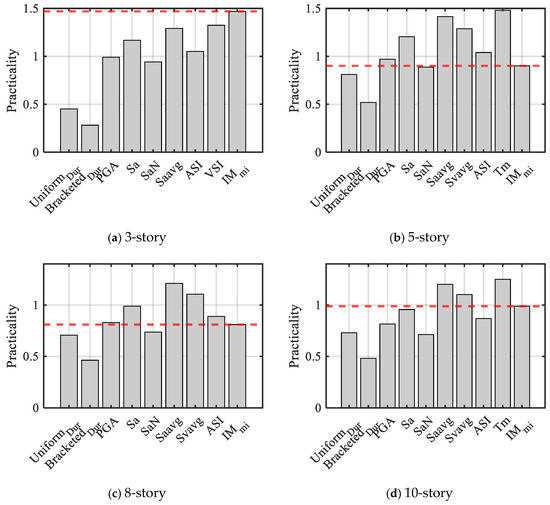
Figure 12.
Practicality of and other scalar parameters (The red dotted line represents the value of ).
5.3.4. Proficiency
To mitigate potential biases or contradictions from evaluating effectiveness and practicality separately, proficiency has been proposed as an evaluation criterion that combines the advantages of efficiency and practicality [57]. Proficiency is defined as the ratio of efficiency to practicality b, according to Equation (18). Typically, a more proficient IM indicates a reduced modified dispersion, which represents the degree of EDP’s uncertainty.
As a comprehensive indicator for IM evaluation, Figure 13 demonstrates that Sa, Saavg, Svavg, VSI, and exhibit superior proficiency. Notably, and Svvag exhibit optimal benefit ratio performance for different structures. Similarly to compound IMs in formulation, Svavg can also be considered a compound IM. The superior performance of these two IMs indicates that employing compound IMs for structural demand estimation enhances the reliability of fragility and risk assessments. In accordance with correlation and effectiveness measures, Sa, Saavg, Svavg, and VSI exhibit reduced ζ values and enhanced proficiency. Considering all structural seismic demand model evaluation parameters, emerges as a potentially superior intensity measure, since compound IMs enable more comprehensive consideration of ground motion features.
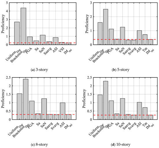
Figure 13.
Proficiency of and other scalar parameters (The red dotted line represents the value of ).
5.3.5. Sufficiency
In linear regression analysis, sufficiency typically refers to whether a model fully utilizes available data information for optimal prediction. For the seismic demand models in this study, particular attention should be paid to potential omission of significant explanatory variables such as seismic characteristics (magnitude M and epicentral distance R). A sufficient IM should exhibit independence from M and R. Residual analysis was conducted to investigate the sufficiency of the compound intensity measure with respect to M and R, where residuals are defined as differences between predicted values from fitted curves and actual demand values.
Linear regression analysis of the residual results versus the magnitude M was performed for each of the four structures, and the linear regression results are shown in Figure 14. The goodness of fit for the four structural residuals relative to the fitted straight line of magnitude M is below 0.01, whereas the goodness of fit for the residuals of the three-story and eight-story structures is approximately 0.001. The absolute values of the slopes of the fitted straight lines are minimal, measuring at 0.001, 0.002, 0.001, and 0.002, and are nearly zero, indicating that the variations in magnitude M exert relatively minor impacts on residual outcomes.
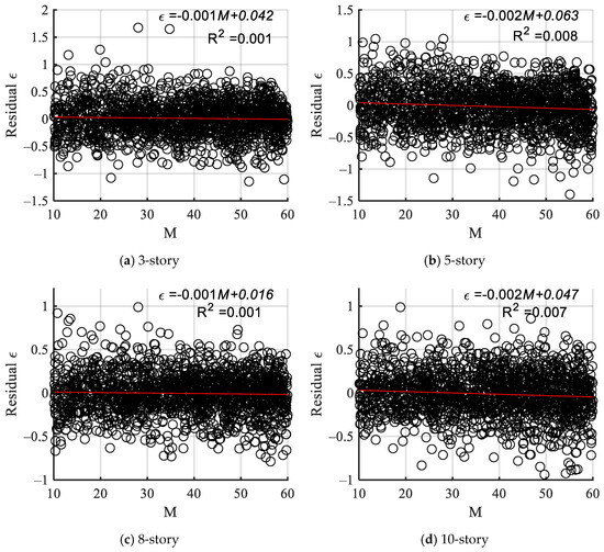
Figure 14.
Linear regression analysis of residuals ε and magnitude M.
Linear regression of residuals of the four structures with respect to the epicenter distance R was performed, and the linear regression results are shown in Figure 15. The goodness-of-fit for the fitted lines of the residuals of the four structures in relation to the epicentral distance R is below 0.01, indicating a lack of significance, whereas the goodness-of-fit for the fitted line of the five-story structure approaches 0. The absolute values of the slopes of the fitted lines of the residuals for the four structures with respect to the epicentral distance R are close to 0, which indicates that variations in the epicentral distance R have a minimal impact on the residuals’ results. The results indicate that the magnitude M and the epicenter distance R exert minimal influence on the residuals, suggesting that is independent of both the magnitude and epicenter distance with satisfactory sufficiency.
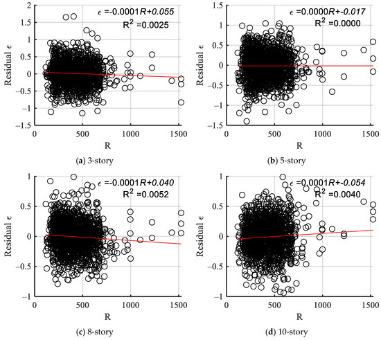
Figure 15.
Linear regression analysis of residuals ε and fault distance R.
6. Conclusions
This study employs a feature selection method to determine the optimal subset of features for fragility analysis and seismic demand modeling. Pearson correlation analysis is employed for the preliminary selection of features, followed by a mutually informative feature selection algorithm that accounts for correlation, redundancy, and complementarity to determine the subset of ground motion features for the construction of compound intensity measures. Four multi-story RC frame structures are studied to demonstrate and discuss the proposed method. The following conclusions are obtained:
- The coefficient of determination for the multivariate linear regression model, as determined by several mutual information feature selection procedures, surpasses 0.9, indicating a strong match to the data. Comparison with the partial least squares regression model demonstrates that the features identified using mutual information metrics possess a robust capaci.y to explain seismic demand factor parameters and are suitable for analyzing structural seismic fragility.
- The probabilistic demand model was examined with linear regression analysis, utilizing compound intensity measures and various scalar intensity measures with engineering demand parameters. The goodness-of-fit results indicate that the derived from the mutual information method exceeds the other IMs, demonstrating superior fit.
- The compound IM was compared with other scalar IMs using correlation, efficiency, proficiency, and sufficiency as evaluation criteria. In general, the evaluation results indicate that the compound IM is more suitable as a ground motion intensity measure compared to other scalar IMs. The compound IM can analyze ground motion parameters more comprehensively, diminish data dispersion, and enhance predictive accuracy.
- The goodness of fit of the four structural residual results with the fitted straight line of magnitude M indicates that both magnitude M and epicenter distance R exert minimal influence on the residuals. It indicates that the compound IM is independent of magnitude and epicenter distance with good sufficiency.
The method proposed in this paper is not only applicable to reinforced concrete frame structures but can also be used for fragility analysis and the selection of feature parameters for other structures.
Author Contributions
Conceptualization, Z.S. and X.L.; methodology, Z.S.; software, Z.S.; validation, X.L., Y.W., Z.S. and B.Z.; formal analysis, Z.S.; investigation, Z.S.; resources, X.L. and B.Z.; data curation, Z.S.; writing—original draft preparation, Z.S.; writing—review and editing, X.L. and Y.W.; visualization, Z.S.; supervision, X.L. and Y.W.; project administration, X.L.; funding acquisition, X.L. and B.Z. All authors have read and agreed to the published version of the manuscript.
Funding
This research was funded by National Key R&D Program of China (2023YFC3007400); Shanghai Science and Technology Plan Project, China (Grant Nos. 22dz1200200 and 22dz1201400).
Data Availability Statement
The data and original contributions presented in the study are included in the article, further inquiries can be directed to the corresponding author.
Conflicts of Interest
Author Bochang Zhou was employed by the company Shanghai Earthquake Administration. The remaining authors declare that the research was conducted in the absence of any commercial or financial relationships that could be construed as a potential conflict of interest.
References
- Meral, E. Relationships between ground motion parameters and energy demands for regular low-rise RC frame buildings. Bull. Earthq. Eng. 2024, 22, 2829–2865. [Google Scholar] [CrossRef]
- Vamvatsikos, D.; Cornell, C.A. Incremental dynamic analysis. Earthq. Eng. Struct. Dyn. 2002, 31, 491–514. [Google Scholar] [CrossRef]
- Baker, J.W. Efficient Analytical Fragility Function Fitting Using Dynamic Structural Analysis. Earthq. Spectra 2015, 31, 579–599. [Google Scholar] [CrossRef]
- Eslamnia, H.; Malekzadeh, H.; Jalali, S.A.; Moghadam, A.S. Seismic energy demands and optimal intensity measures for continuous concrete box-girder bridges. Soil Dyn. Earthq. Eng. 2023, 165, 107657. [Google Scholar] [CrossRef]
- Du, M.; Zhang, S.R.; Wang, C.; Li, Z.; Yao, J.; Lu, T. Development of the compound intensity measure and seismic performance assessment for aqueduct structures considering fluid-structure interaction. Ocean. Eng. 2024, 311, 118838. [Google Scholar] [CrossRef]
- Yan, Y.; Xia, Y.; Yang, J.; Sun, L. Optimal selection of scalar and vector-valued seismic intensity measures based on Gaussian Process Regression. Soil Dyn. Earthq. Eng. 2022, 152, 106961. [Google Scholar] [CrossRef]
- Li, B.; Cai, Z. Effectiveness of vector intensity measures in probabilistic seismic demand assessment. Soil Dyn. Earthq. Eng. 2022, 155, 107201. [Google Scholar] [CrossRef]
- Kiani, J.; Camp, C.; Pezeshk, S. The importance of non-spectral intensity measures on the risk-based structural responses. Soil Dyn. Earthq. Eng. 2019, 120, 97–112. [Google Scholar] [CrossRef]
- Elenas, A.; Meskouris, K. Correlation study between seismic acceleration parameters and damage indices of structures. Eng. Struct. 2001, 23, 698–704. [Google Scholar] [CrossRef]
- Akkar, S.; Ozen, O. Effect of peak ground velocity on deformation demands for SDOF systems. Earthq. Eng. Struct. Dyn. 2005, 34, 1551–1571. [Google Scholar] [CrossRef]
- Sun, B.B.; Deng, M.J.; Zhang, S.R.; Wang, C.; Cui, W.; Li, Q.; Xu, J.; Zhao, X.H.; Yan, H.H. Optimal selection of scalar and vector-valued intensity measures for improved fragility analysis in cross-fault hydraulic tunnels. Tunn. Undergr. Space Technol. 2023, 132, 104857. [Google Scholar] [CrossRef]
- Shome, N.; Cornell, C.A.; Bazzurro, P.; Carballo, J.E. Earthquakes, Records, and Nonlinear Responses. Earthq. Spectra 1998, 14, 469–500. [Google Scholar] [CrossRef]
- Luco, N.; Cornell, C.A. Structure-specific scalar intensity measures for near-source and ordinary earthquake ground motions. Earthq. Spectra 2007, 23, 357–392. [Google Scholar] [CrossRef]
- Eads, L.; Miranda, E.; Lignos, D.G. Average spectral acceleration as an intensity measure for collapse risk assessment. Earthq. Eng. Struct. Dyn. 2015, 44, 2057–2073. [Google Scholar] [CrossRef]
- Adam, C.; Kampenhuber, D.; Ibarra, L.F.; Tsantaki, S. Optimal Spectral Acceleration-based Intensity Measure for Seismic Collapse Assessment of P-Delta Vulnerable Frame Structures. J. Earthq. Eng. 2017, 21, 1189–1195. [Google Scholar] [CrossRef]
- Baker, J.W. Probabilistic structural response assessment using vector-valued intensity measures. Earthq. Eng. Struct. Dyn. 2007, 36, 1861–1883. [Google Scholar] [CrossRef]
- Vamvatsikos, D.; Cornell, C.A. Developing efficient scalar and vector intensity measures for IDA capacity estimation by incorporating elastic spectral shape information. Earthq. Eng. Struct. Dyn. 2005, 34, 1573–1600. [Google Scholar] [CrossRef]
- Vargas-Alzate, Y.F.; Hurtado, J.E.; Pujades, L.G. New insights into the relationship between seismic intensity measures and nonlinear structural response. Bull. Earthq. Eng. 2022, 20, 2329–2365. [Google Scholar] [CrossRef]
- Baker, J.W.; Cornell, C.A. A vector-valued ground motion intensity measure consisting of spectral acceleration and epsilon. Earthq. Eng. Struct. Dyn. 2005, 34, 1193–1217. [Google Scholar] [CrossRef]
- Modica, A.; Stafford, P.J. Vector fragility surfaces for reinforced concrete frames in Europe. Bull. Earthq. Eng. 2014, 12, 1725–1753. [Google Scholar] [CrossRef]
- Marco, F.; André, R.B.; Joel, P.C.; Enrico, S.; José, I.R. Probabilistic seismic response analysis of a 3-D reinforced concrete building. Struct. Saf. 2013, 44, 11–27. [Google Scholar] [CrossRef]
- Kohrangi, M.; Bazzurro, P.; Vamvatsikos, D. Conditional spectrum bidirectional record selection for risk assessment of 3D structures using scalar and vector IMs. Earthq. Eng. Struct. Dyn. 2019, 48, 1066–1082. [Google Scholar] [CrossRef]
- Bojorquez, E.; Iervolino, I.; Reyes-Salazar, A.; Ruiz, S.E. Comparing vector-valued intensity measures for fragility analysis of steel frames in the case of narrow-band ground motions. Eng. Struct. 2012, 45, 472–480. [Google Scholar] [CrossRef]
- Kohrangi, M.; Bazzurro, P.; Vamvatsikos, D. Vector and Scalar IMs in Structural Response Estimation: Part II—Building Demand Assessment. Earthq. Spectra 2016, 32, 1525–1543. [Google Scholar] [CrossRef]
- Luis, A.P.; Yeudy, F.V.-A.; Luis, G.P.; Sergio, A.D. A drift-correlated ground motion intensity measure: Application to steel frame buildings. Soil Dyn. Earthq. Eng. 2020, 132, 106096. [Google Scholar] [CrossRef]
- Liu, T.T.; Yu, X.H.; Lu, D.G. An Approach to Develop Compound Intensity Measures for Prediction of Damage Potential of Earthquake Records Using Canonical Correlation Analysis. J. Earthq. Eng. 2020, 24, 1747–1770. [Google Scholar] [CrossRef]
- Liu, B.; Hu, J.; Xie, L. Exploratory factor analysis-based method to develop compound intensity measures for predicting potential structural damage of ground motion. Bull. Earthq. Eng. 2022, 20, 7107–7135. [Google Scholar] [CrossRef]
- Liu, T.-T.; Lu, D.-G.; Yu, X.-H. Development of a compound intensity measure using partial least-squares regression and its statistical evaluation based on probabilistic seismic demand analysis. Soil Dyn. Earthq. Eng. 2019, 125, 105725. [Google Scholar] [CrossRef]
- Sun, B.B.; Liu, W.Y.; Deng, M.J.; Zhang, S.R.; Wang, C.; Guo, J.J.; Wang, J.; Wang, J.Y. Compound intensity measures for improved seismic performance assessment in cross-fault hydraulic tunnels using partial least-squares methodology. Tunn. Undergr. Space Technol. 2023, 132, 104890. [Google Scholar] [CrossRef]
- Chen, Z.; Yu, W.; Zhu, H.; Xie, L. Ranking method of the severest input ground motion for underground structures based on composite ground motion intensity measures. Soil Dyn. Earthq. Eng. 2023, 168, 107828. [Google Scholar] [CrossRef]
- Yong, W.; Zhi, Z.; Duofa, J.; Xiaolan, P.; Aonan, T. Machine learning-driven probabilistic seismic demand model with multiple intensity measures and applicability in seismic fragility analysis for nuclear power plants. Soil Dyn. Earthq. Eng. 2023, 171, 107966. [Google Scholar] [CrossRef]
- Bommer, J.J.; Martínez-Pereira, A. The effective duration of earthquake strong motion. J. Earthq. Eng. 1999, 3, 127–172. [Google Scholar] [CrossRef]
- Hansen, R.J. Seismic Design for Nuclear Power Plants; MIT Press: Cambridge, MA, USA, 1970. [Google Scholar]
- Pu, W.; Wu, M.; Huang, B.; Zhang, H. Quantification of response spectra of pulse-like near-fault ground motions. Soil Dyn. Earthq. Eng. 2018, 104, 117–130. [Google Scholar] [CrossRef]
- Kramer, S.L. Geotechnical Earthquake Engineering; Prentice Hall: Hoboken, NJ, USA, 1996. [Google Scholar]
- Mackie, K.R. Fragility-Based Seismic Decision Making for Highway Overpass Bridges. Ph.D. Thesis, University of California, Berkeley, Berkeley, CA, USA, 2004. [Google Scholar]
- Applied Technology Council. Tentative Provisions for the Development of Seismic Regulations for Buildings; ATC-3-06; Applied Technology Council: Redwood City, CA, USA, 1978. [Google Scholar]
- Anderson, J.C.; Bertero, V.V. Uncertainties in Establishing Design Earthquakes. J. Struct. Eng.-Asce 1987, 113, 1709–1724. [Google Scholar] [CrossRef]
- Wu, Z.-N.; Li, Z.-Q.; Dong, Y.; Han, X.-L.; Zhang, G.; Feng, R.; Zhu, K. Seismic intensity measure selection incorporating interaction effects for damage assessment across different structural sensitive regions. Structures 2024, 67, 106917. [Google Scholar] [CrossRef]
- Thun, J.L.V.; Roehm, L.H.; Scott, G.A.; Wilson, J.A. Earthquake ground motions for design and analysis of dams. Geotech. Spec. Publ. 1988, 20, 463–481. [Google Scholar]
- Housner, G.W. Behavior of Structures During Earthquakes. J. Eng. Mech. Div. 1959, 85, 109–129. [Google Scholar] [CrossRef]
- Rathje, E.M.; Abrahamson, N.A.; Bray, J.D. Simplified Frequency Content Estimates of Earthquake Ground Motions. J. Geotech. Geoenvironmental Eng. 1998, 124, 150–159. [Google Scholar] [CrossRef]
- Chen, R.; Sun, N.; Chen, X.; Yang, M.; Wu, Q. Supervised Feature Selection With a Stratified Feature Weighting Method. IEEE Access 2018, 6, 15087–15098. [Google Scholar] [CrossRef]
- Gao, W.; Hu, L.; Zhang, P. Class-specific mutual information variation for feature selection. Pattern Recognit. 2018, 79, 328–339. [Google Scholar] [CrossRef]
- Singh, D.; Singh, B. Hybridization of feature selection and feature weighting for high dimensional data. Appl. Intell. 2019, 49, 1580–1596. [Google Scholar] [CrossRef]
- Gao, W.; Hu, L.; Zhang, P. Feature redundancy term variation for mutual information-based feature selection. Appl. Intell. 2020, 50, 1272–1288. [Google Scholar] [CrossRef]
- Zhao, J.; Zhou, Y.; Zhang, X.; Chen, L. Part mutual information for quantifying direct associations in networks. Proc. Natl. Acad. Sci. USA 2016, 113, 5130–5135. [Google Scholar] [CrossRef] [PubMed]
- Dionisio, A.; Menezes, R.; Mendes, D.A. Mutual information: A measure of dependency for nonlinear time series. Phys. A Stat. Mech. Its Appl. 2004, 344, 326–329. [Google Scholar] [CrossRef]
- Hanchuan, P.; Fuhui, L.; Ding, C. Feature selection based on mutual information criteria of max-dependency, max-relevance, and min-redundancy. IEEE Trans. Pattern Anal. Mach. Intell. 2005, 27, 1226–1238. [Google Scholar] [CrossRef] [PubMed]
- Lin, D.; Tang, X. Conditional Infomax Learning: An Integrated Framework for Feature Extraction and Fusion. In Proceedings of the Computer Vision—ECCV 2006, Graz, Austria, 7–13 May 2006; Springer: Berlin/Heidelberg, Germany, 2006; pp. 68–82. [Google Scholar]
- Gao, W.; Hu, L.; Zhang, P.; He, J. Feature selection considering the composition of feature relevancy. Pattern Recognit. Lett. 2018, 112, 70–74. [Google Scholar] [CrossRef]
- Lai, Q.H.; Hu, J.J.; Xu, L.J.; Xie, L.L.; Lin, S.B. Method for Ranking Pulse-like Ground Motions According to Damage Potential for Reinforced Concrete Frame Structures. Buildings 2022, 12, 754. [Google Scholar] [CrossRef]
- Song, Z.; Li, X.; Wang, Y.; Zhou, B. Amplitude-Scaling Bias Analysis of Ground Motion Record Set in Strip Method for Structural Seismic Fragility Assessment. Buildings 2025, 15, 401. [Google Scholar] [CrossRef]
- McKenna, F.; Fenves, G.; Scott, M.; Jeremic, B. Open System for Earthquake Engineering Simulation (OpenSees); Pacific Earthquake Engineering Research Center, University of California: Berkeley, CA, USA, 2000. [Google Scholar]
- Cornell, C.A.; Jalayer, F.; Hamburger, R.O.; Foutch, D.A. Probabilistic basis for 2000 SAC Federal Emergency Management Agency steel moment frame guidelines. J. Struct. Eng. 2002, 128, 526–533. [Google Scholar] [CrossRef]
- Giovenale, P.; Cornell, C.A.; Esteva, L. Comparing the adequacy of alternative ground motion intensity measures for the estimation of structural responses. Earthq. Eng. Struct. Dyn. 2004, 33, 951–979. [Google Scholar] [CrossRef]
- Padgett, J.E.; Nielson, B.G.; DesRoches, R. Selection of optimal intensity measures in probabilistic seismic demand models of highway bridge portfolios. Earthq. Eng. Struct. Dyn. 2008, 37, 711–725. [Google Scholar] [CrossRef]
Disclaimer/Publisher’s Note: The statements, opinions and data contained in all publications are solely those of the individual author(s) and contributor(s) and not of MDPI and/or the editor(s). MDPI and/or the editor(s) disclaim responsibility for any injury to people or property resulting from any ideas, methods, instructions or products referred to in the content. |
© 2025 by the authors. Licensee MDPI, Basel, Switzerland. This article is an open access article distributed under the terms and conditions of the Creative Commons Attribution (CC BY) license (https://creativecommons.org/licenses/by/4.0/).