
Optimization of Actuator Arrangement of Cable–Strut Tension Structures Based on Multi-Population Genetic Algorithm

Abstract
1. Introduction
2. Materials and Methods
2.1. Structural Controllability Optimization via Weighted Sensitivity
2.1.1. Fundamental Assumptions
- (1)
- All nodes are idealized as frictionless hinged nodes.
- (2)
- Cable elements sustain axial tension only while strut elements sustain axial compression only.
- (3)
- The structure is subjected exclusively to nodal loads.
- (4)
- The cross-sectional area of each member remains constant throughout the calculation.
- (5)
- Cable and strut materials are idealized elastic bodies, and their constitutive relationships obey Hooke’s Law.
- (6)
- For active members embedded with actuators (as shown in Figure 1), the axial stiffness k is determined as follows.
2.1.2. Weighted Sensitivity Index Formulation
2.1.3. Governing Equation Derivation and Actuator Quantity Analysis
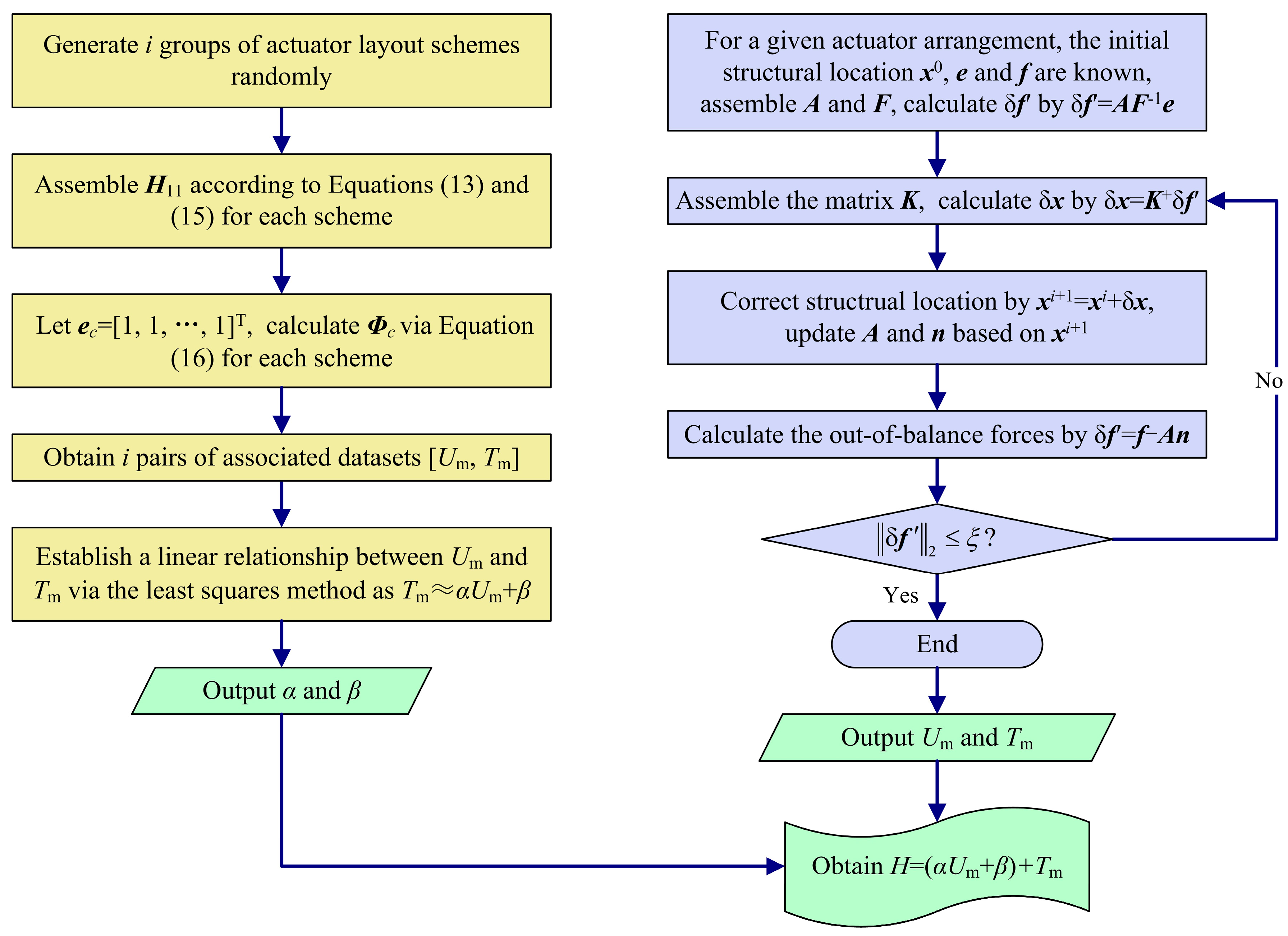
2.1.4. Nonlinear Iterative Refinement of Sensitivity Indices
2.2. Structural Controllability Optimization via System Strain Energy Criterion
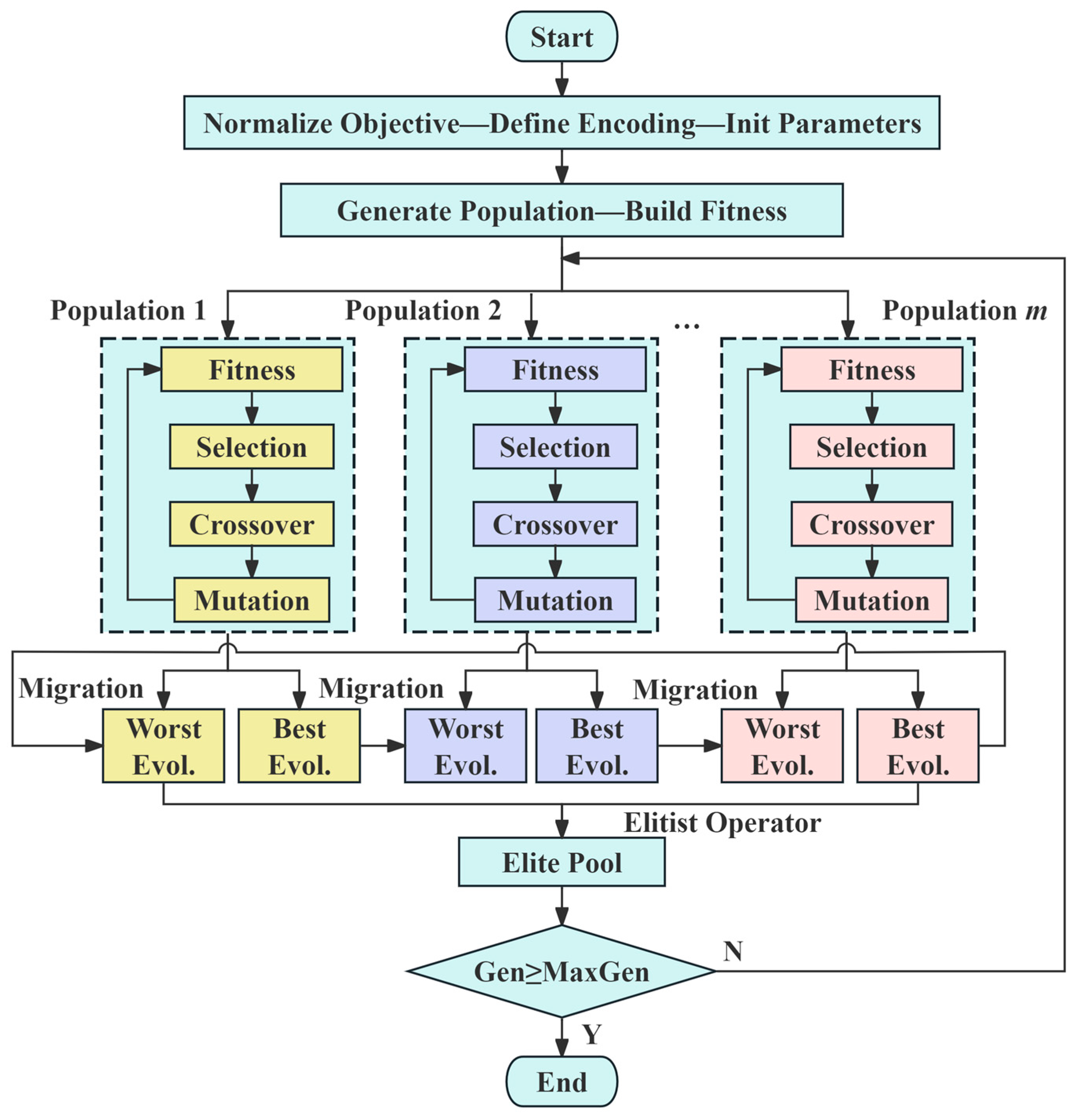
2.3. Multiple Population Genetic Algorithms
3. Results and Examples
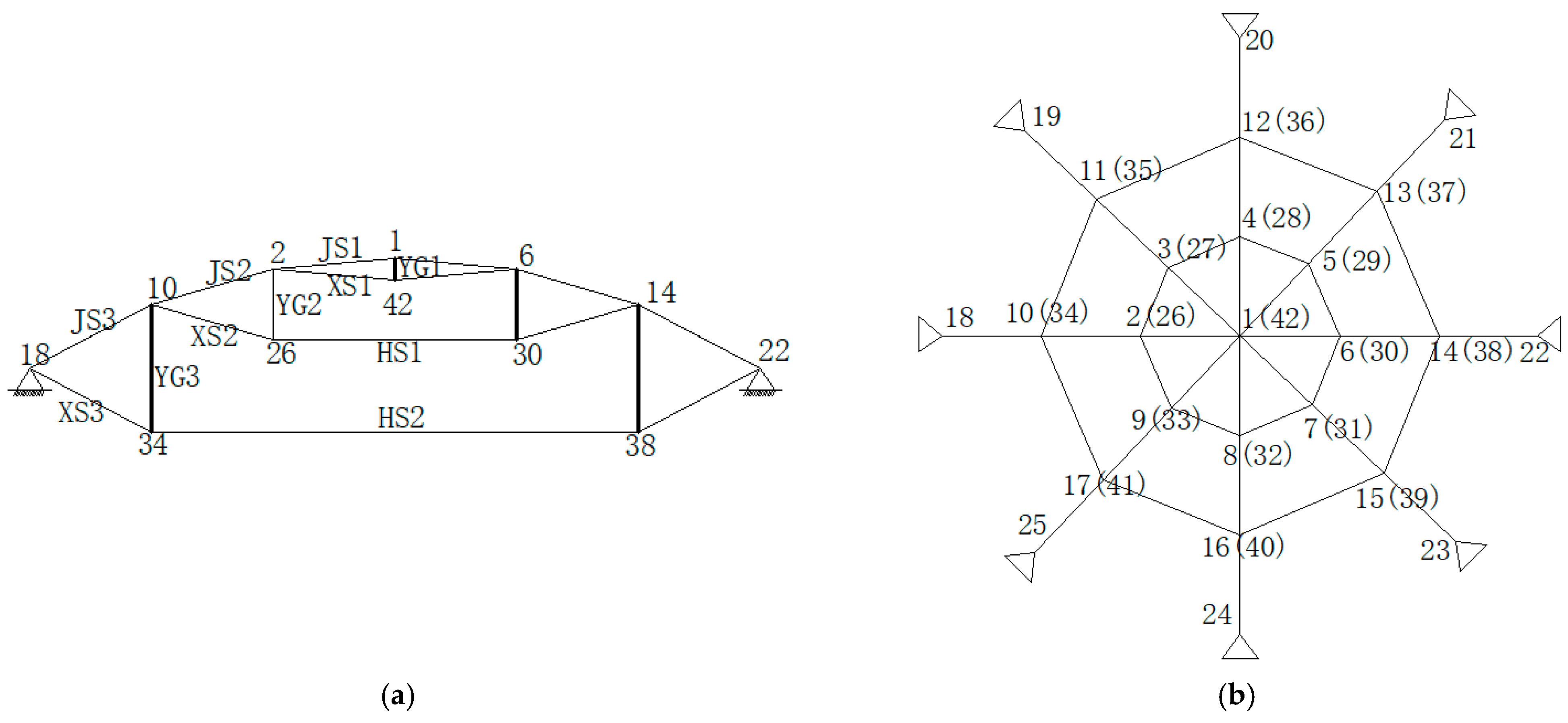
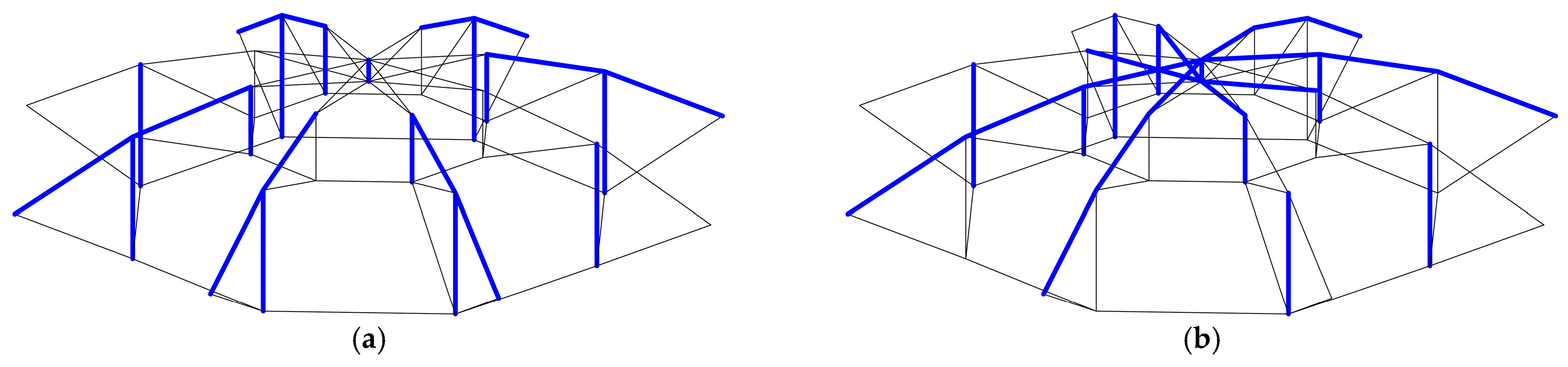
3.1. Geiger Cable Dome
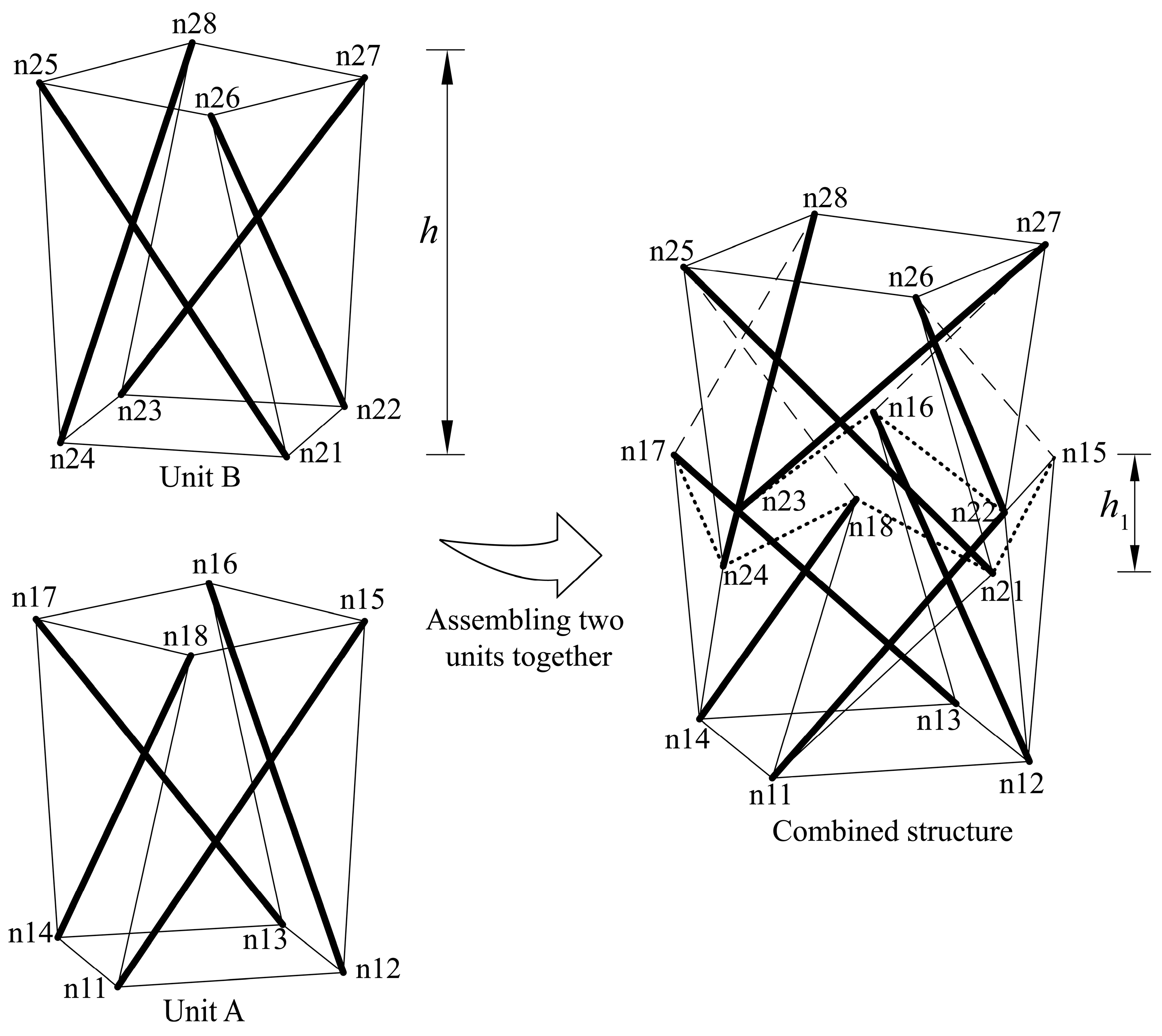
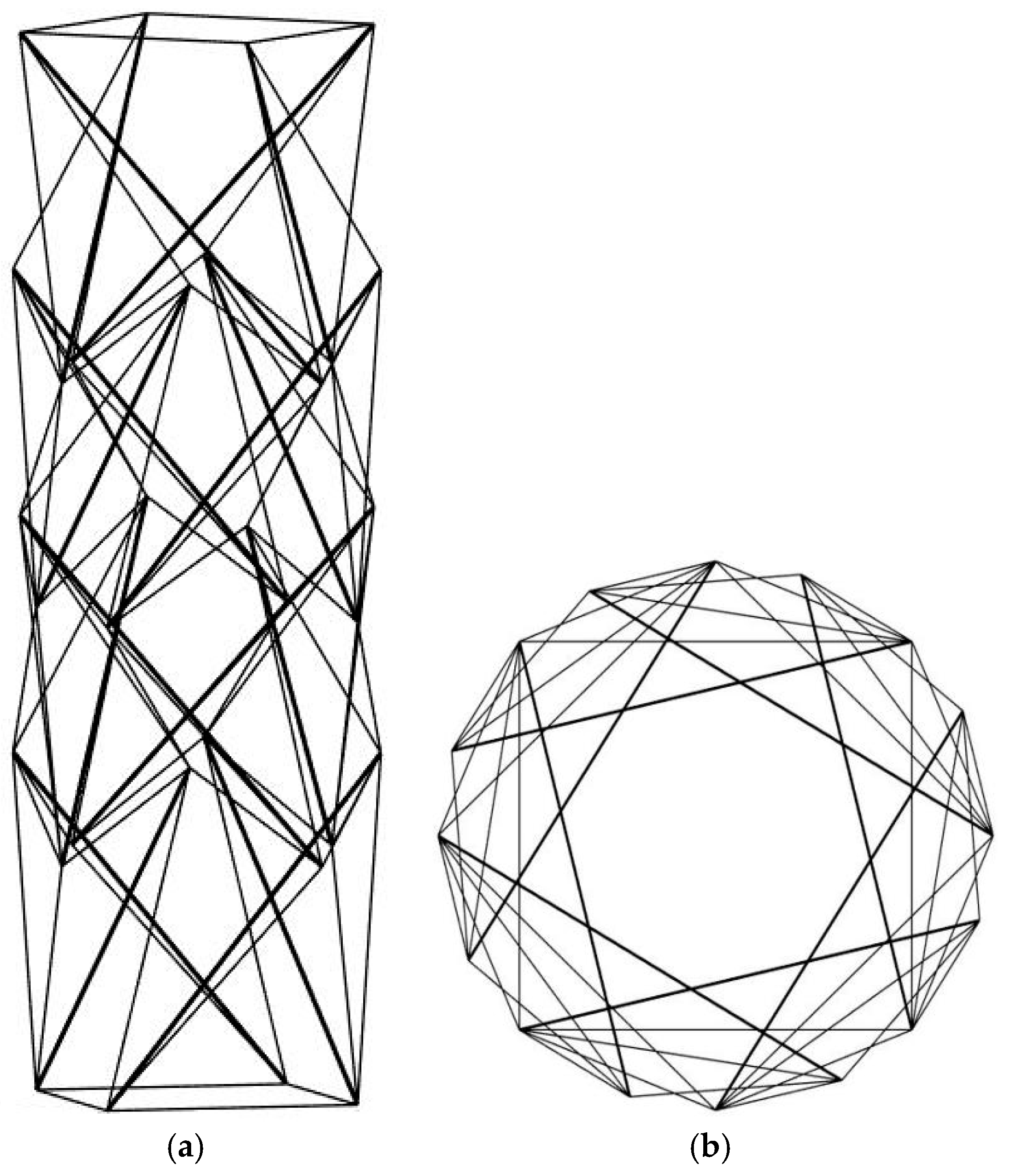
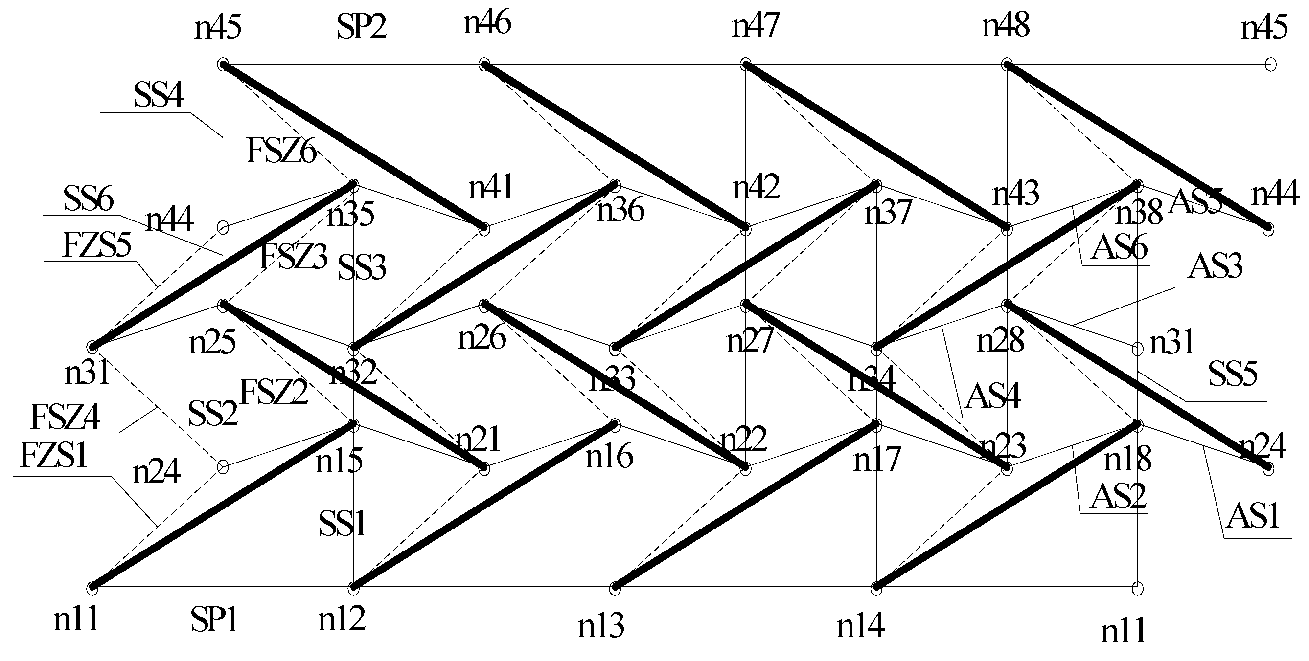
3.2. Tensegrity Structure
4. Conclusions
Author Contributions
Funding
Data Availability Statement
Conflicts of Interest
References
- Guest, S. The stiffness of prestressed frameworks: A unifying approach. Int. J. Solids Struct. 2006, 43, 842–854. [Google Scholar] [CrossRef]
- Obara, P.; Tomasik, J. Active control of stiffness of tensegrity plate-like structures built with simplex modules. Materials 2021, 14, 7888. [Google Scholar] [CrossRef] [PubMed]
- Lin, F.; Chen, J.; Chen, C.; Chen, M.; Dong, Z.; Zhou, J. Deployment accuracy analysis of cable-strut deployable mechanism with joint clearances and forces constrained. J. Vibroengineering 2018, 20, 2085–2098. [Google Scholar] [CrossRef]
- Rezaiee-Pajand, M.; Masoodi, A.R.; Arabi, E. Geometric and Material Nonlinear Analyses of Trusses Subjected to Thermomechanical Loads. Struct. Eng. Int. 2022, 33, 302–313. [Google Scholar] [CrossRef]
- Moored, K.W.; Bart-Smith, H. Investigation of clustered actuation in tensegrity structures. Int. J. Solids Struct. 2009, 46, 3272–3281. [Google Scholar] [CrossRef]
- Zhang, P.; Feng, J. Initial prestress design and optimization of tensegrity systems based on symmetry and stiffness. Int. J. Solids Struct. 2017, 106–107, 68–90. [Google Scholar] [CrossRef]
- Zhang, H.; Lu, J.; Gong, P.; Li, N. Mechanical properties and shape-control abilities of a cable dome under asymmetrical loads. J. Constr. Steel Res. 2023, 208, 108021. [Google Scholar] [CrossRef]
- Raja, M.G.; Narayanan, S. Vibration control of tensegrity structures using different active control strategies. J. Vib. Control 2015, 21, 3–20. [Google Scholar] [CrossRef]
- Hrabaka, M.; Bulin, R.; Hajman, M. New actuation planning method for the analysis and design of active tensegrity structures. Eng. Struct. 2023, 293, 116597. [Google Scholar] [CrossRef]
- Li, S.; Xiao, N.; Dong, S. Sensitivity analysis on responses of adaptive cable-struttensile structure with length changeable elements. J. Huazhong Univ. Sci. Technol. (Nat. Sci. Ed.) 2014, 42, 119–123. [Google Scholar]
- Goyal, R.; Majji, M.; Skelton, R.E. Integrating structure, information architecture and control design: Application to tensegrity systems. Mech. Syst. Signal Process. 2021, 161, 107913. [Google Scholar] [CrossRef]
- Zou, J.; Lu, J.; Li, N.; Zhang, H.; Sha, Z.; Xu, Z. Control accuracy and sensitivity of a double rhombic-strut adaptive beam string structure. J. Constr. Steel Res. 2025, 224, 109166. [Google Scholar] [CrossRef]
- Lu, R.; Zhang, H.; Zhang, Q.; Jiang, H.; Feng, J.; Meloni, M.; Cai, J. Machine learning-based active control for lightweight antenna with force density method and nested genetic algorithm. Thin-Walled Struct. 2024, 203, 112212. [Google Scholar] [CrossRef]
- Sui, Y.; Shao, J. Research on strength control for adaptive structure under multi-loading cases. Chin. J. Theor. Appl. Mech. 2002, 34, 223–228. [Google Scholar]
- Veuve, N.; Dalil Safaei, S.; Smith, I.F.C. Active control for mid-span connection of a deployable tensegrity footbridge. Eng. Struct. 2016, 112, 245–255. [Google Scholar] [CrossRef]
- Feng, X.; Fan, Y.; Peng, H.; Chen, Y.; Zheng, Y. Optimal Active Vibration Control of Tensegrity Structures Using Fast Model Predictive Control Strategy. Struct. Control Health Monit. 2023, 2023, 2076738. [Google Scholar] [CrossRef]
- Kripakaran, P.; Smith, I.F.C. Configuring and enhancing measurement systems for damage identification. Adv. Eng. Inform. 2009, 23, 424–432. [Google Scholar] [CrossRef]
- Hieu, Q.B.; Kawabata, M.; Nguyen, C.V. A combination of genetic algorithm and dynamic relaxation method for practical form-finding of tensegrity structures. Adv. Struct. Eng. 2022, 25, 2237–2254. [Google Scholar]
- Zhang, P.; Kawaguchi, K.; Feng, J. Prismatic tensegrity structures with additional cables: Integral symmetric states of self-stress and cable-controlled reconfiguration procedure. Int. J. Solids Struct. 2014, 51, 4294–4306. [Google Scholar] [CrossRef]
- Feng, X.; Ou, Y.; Miah, M.S. Energy-based comparative analysis of optimal active control schemes for clustered tensegrity structures. Struct. Control Health Monit. 2018, 25, e2215. [Google Scholar] [CrossRef]
- Ma, S.; Chen, M.; Skelton, R.E. Dynamics and control of clustered tensegrity systems. Eng. Struct. 2022, 264, 114391. [Google Scholar] [CrossRef]
- Chen, Y.; Zhou, H.; Gao, J.; Shen, Z.; Xie, T.; Sareh, P. Accurate force evaluation in prestressed cable-strut structures: A robust sparse Bayesian learning method with feedback-driven error optimization. Eng. Struct. 2025, 330, 119878. [Google Scholar] [CrossRef]
- Zhang, P.; Xiong, H.T.; Chen, J.S. Unified Fundamental Formulas for Static Analysis of Pin-Jointed Bar Assemblies. Symmetry 2020, 12, 994. [Google Scholar] [CrossRef]
- Zhang, P.; Zhou, J.K.; Chen, J.S. Form-finding of complex tensegrity structures using constrained optimization method. Compos. Struct. 2021, 268, 113971. [Google Scholar] [CrossRef]
- Pellegrino, S. Structural computations with the singular value decomposition of the equilibrium matrix. Int. J. Solids Struct. 1993, 30, 3025–3035. [Google Scholar] [CrossRef]
- Chen, Y.; Yan, J.; Chen, Y.; Sareh, P.; Feng, J. Feasible prestress modes for cable-strut structures with multiple self-stress states using Particle Swarm Optimization. J. Comput. Civ. Eng. 2020, 34, 04020003. [Google Scholar] [CrossRef]
- Zhang, P.; Fan, W.; Chen, Y.; Feng, J.; Sareh, P. Structural symmetry recognition in planar structures using Convolutional Neural Networks. Eng. Struct. 2022, 260, 114227. [Google Scholar] [CrossRef]


| Existing Techniques | Proposed Approach |
|---|---|
| Single controllability metrics | Dual-criteria framework: Combine weighted sensitivity (local control) and system strain energy (global stiffness balance) |
| Risk of actuator over-concentration | Variance-constrained sensitivity: Avoid actuator over-concentration through displacement/internal force variance thresholds |
| Standard GA/PSO algorithms | MPGA algorithm: Adaptive crossover/mutation probabilities and migration operators enhance exploration–exploitation balance |
| Limited validation scope | Comprehensive validation: Tested on Geiger cable dome and multi-layer tensegrity structure, demonstrating scalability and robustness |
| Member Group | Prestress | Member Group | Prestress | Member Group | Prestress |
|---|---|---|---|---|---|
| JS1 | 9.3752 | XS1 | 9.3752 | YG1 | −5.8994 |
| JS2 | 19.4234 | XS2 | 19.3115 | YG2 | −5.3538 |
| JS3 | 41.9695 | XS3 | 41.9695 | YG3 | −19.3832 |
| HS1 | 24.2426 | HS2 | 48.6374 |
| Parameter Name | Parameter Value | Parameter Name | Parameter Value |
|---|---|---|---|
| Number of populations (s) | 4 | Size of Single Population (m) | 40 |
| Minimum Retained Generations | 15 | Baseline crossover probability (Pa) | 0.9 |
| Mutation Probability in later stage (Pm) | 0.1 | Penalty factor | 0.6 |
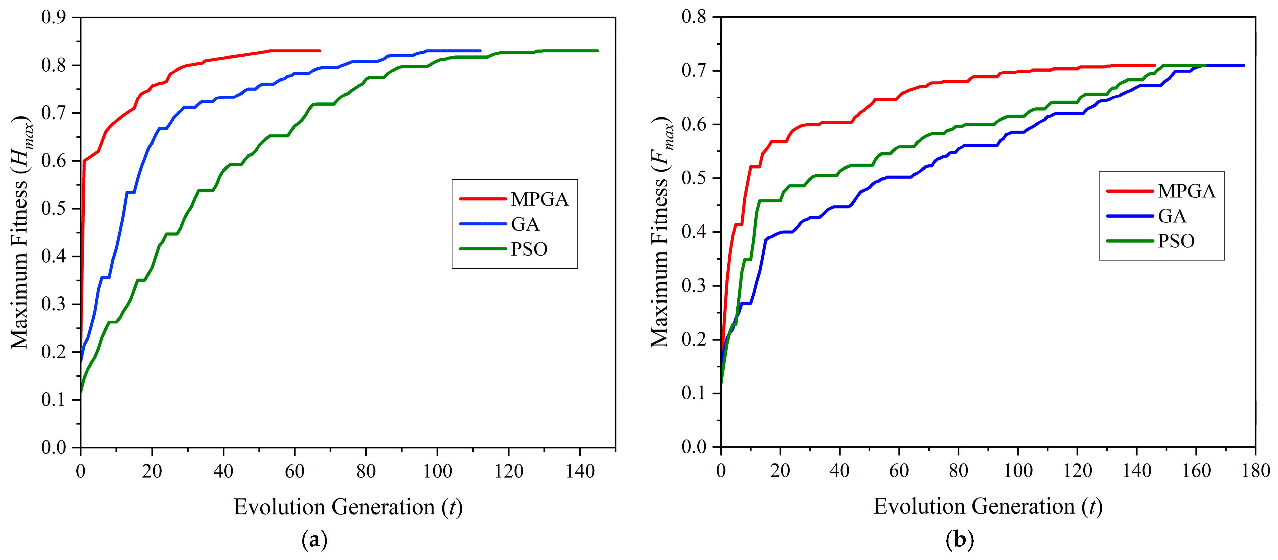
| Model | Algorithm | Convergence Count/100 Runs | Average Convergence Generation | Fastest Convergence Generation |
|---|---|---|---|---|
| Model 1 | MPGA | 72 | 68 | 53 |
| GA | 37 | 131 | 97 | |
| PSO | 18 | 172 | 130 | |
| Model 2 | MPGA | 78 | 151 | 132 |
| GA | 28 | 186 | 162 | |
| PSO | 18 | 176 | 149 |
| Model Number | 1 | 2 | 3 | 4 | 5 | 6 | 7 | 8 | 9 |
| Model 1 | 3.77 | 4.00 | 1.37 | 4.00 | 3.71 | 4.00 | 1.37 | 4.00 | 3.71 |
| Model 2 | 3.57 | 2.10 | −1.75 | −4.16 | 4.52 | 2.10 | −1.75 | −4.16 | 4.52 |
| Model Number | 10 | 11 | 12 | 13 | 14 | 15 | 16 | 17 | |
| Model 1 | 2.53 | −1.27 | 2.53 | 3.07 | 2.53 | −1.27 | 2.53 | 3.07 | |
| Model 2 | 5.12 | −3.52 | 1.95 | 2.44 | 5.12 | −3.52 | 1.95 | 2.44 |
| Model Number | JS1 Group | |||||||
| 1–2 | 1–3 | 1–4 | 1–5 | 1–6 | 1–7 | 1–8 | 1–9 | |
| Model 1 | −5.72 | 6.09 | −5.72 | −5.16 | −5.72 | 6.09 | −5.72 | −5.16 |
| Model 2 | −3.04 | −3.23 | 4.01 | 3.54 | −3.04 | −3.23 | 4.01 | 3.54 |
| Model Number | XS1 Group | |||||||
| 2–42 | 3–42 | 4–42 | 5–42 | 6–42 | 7–42 | 8–42 | 9–42 | |
| Model 1 | 0.22 | −1.75 | 0.22 | −0.01 | 0.22 | −1.75 | 0.22 | −0.01 |
| Model 2 | −1.47 | 2.65 | −1.47 | −1.04 | −1.47 | 2.65 | −1.47 | −1.04 |
| Model Number | HS1 Group | |||||||
| 26–27 | 27–28 | 28–29 | 29–30 | 30–31 | 31–32 | 32–33 | 33–26 | |
| Model 1 | −0.72 | −0.72 | −0.73 | −0.73 | −0.72 | −0.72 | −0.73 | −0.73 |
| Model 2 | 1.74 | 2.70 | 0.86 | 2.70 | 1.74 | 2.70 | 0.86 | 2.70 |
| Model Number | YG2 Group | |||||||
| 2–26 | 3–27 | 4–28 | 5–29 | 6–30 | 7–31 | 8–32 | 9–33 | |
| Model 1 | 0.17 | 0.14 | 0.17 | 0.49 | 0.17 | 0.14 | 0.17 | 0.49 |
| Model 2 | −0.49 | 2.56 | −1.32 | −2.33 | −0.49 | 2.56 | −1.32 | −2.33 |
| Member Group | Prestress | Member Group | Prestress | Member Group | Prestress |
|---|---|---|---|---|---|
| YG1, YG4 | −212.55 | AS5, AS6 | 159.94 | SS1, SS4 | 73.81 |
| YG2, YG3 | −253.61 | FZS1, FZS6 | 101.75 | SS1, SS4 | 62.35 |
| AS1, AS2 | 181.53 | FZS2, FZS5 | 1.73 | SS1, SS4 | 128.15 |
| AS3, AS4 | 209.47 | FZS3, FZS4 | 4.15 | SPS2 | 62.49 |
| Parameter Name | Parameter Value | Parameter Name | Parameter Value |
|---|---|---|---|
| Number of populations (s) | 4 | Size of Single Population (m) | 60 |
| Minimum Retained Generations | 15 | Baseline crossover probability (Pa) | 0.8 |
| Mutation Probability in later stage (Pm) | 0.08 | Penalty factor | 0.6 |
| Model Number | Actuator Arrangement | ||||
|---|---|---|---|---|---|
| Model 1 | YG3 | SS1 | SS4 | SS5 | SS6 |
| Model 2 | YG3 | YG4 | AS1 | AS3 | SS6 |
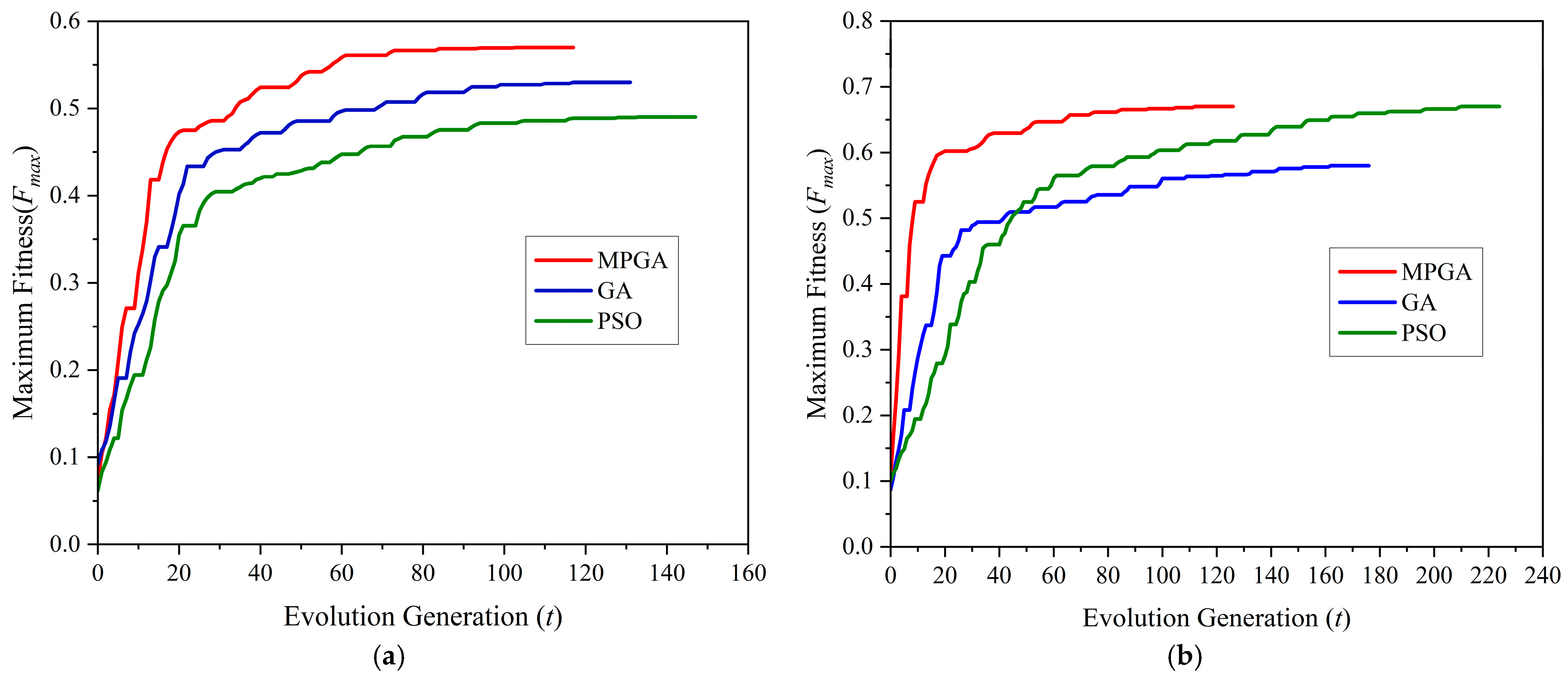
| Model | Algorithm | Convergence Count/100 Runs | Maximum Fitness | Fastest Convergence Generation |
|---|---|---|---|---|
| Model 1 | MPGA | 64 | 0.57 | 103 |
| GA | / | 0.53 | / | |
| PSO | / | 0.49 | / | |
| Model 2 | MPGA | 64 | 0.67 | 112 |
| GA | / | 0.58 | 162 | |
| PSO | 9 | 0.67 | 210 |
| Model Number | 15 to 18 | 21 to 24 | 25 to 28 | 31 to 34 | 35 to 38 | 41 to 44 | 45 to 48 |
|---|---|---|---|---|---|---|---|
| Model 1 | −0.55 | −1.27 | −0.97 | −0.13 | 1.71 | 2.25 | −7.26 |
| Model 2 | −1.95 | −2.84 | −3.29 | −3.99 | −4.37 | −4.12 | 5.18 |
| Model Number | YG1 | YG2 | YG3 | YG4 | AS1 | AS2 | AS3 | AS4 |
| Model 1 | −9.79 | −1.41 | 8.65 | 0.93 | 11.10 | 7.45 | −1.28 | 4.32 |
| Model 2 | −13.53 | −11.24 | 4.28 | 13.05 | 8.98 | −6.10 | −6.91 | 7.82 |
| Model Number | AS5 | AS6 | FZS1 | FZS2 | FZS3 | FZS4 | FZS5 | FZS6 |
| Model 1 | 4.04 | 5.86 | 16.24 | 18.73 | −15.53 | −13.41 | 15.66 | −2.59 |
| Model 2 | −2.26 | −16.83 | 10.12 | 14.32 | 11.59 | −9.62 | 11.33 | −3.42 |
| Model Number | SS1 | SS2 | SS3 | SS4 | SS5 | SS6 | SP1 | |
| Model 1 | 5.23 | 0.84 | −3.22 | 1.23 | 12.34 | 16.86 | 0.26 | |
| Model 2 | 6.37 | 2.45 | −1.48 | −6.80 | −3.35 | −20.59 | −4.37 |
Disclaimer/Publisher’s Note: The statements, opinions and data contained in all publications are solely those of the individual author(s) and contributor(s) and not of MDPI and/or the editor(s). MDPI and/or the editor(s) disclaim responsibility for any injury to people or property resulting from any ideas, methods, instructions or products referred to in the content. |
© 2025 by the authors. Licensee MDPI, Basel, Switzerland. This article is an open access article distributed under the terms and conditions of the Creative Commons Attribution (CC BY) license (https://creativecommons.org/licenses/by/4.0/).
Share and Cite
Xiong, H.; Zhou, T.; Zhang, P.; Shang, Z.; Biswas, M.; Li, H.; Zhu, H. Optimization of Actuator Arrangement of Cable–Strut Tension Structures Based on Multi-Population Genetic Algorithm. Symmetry 2025, 17, 695. https://doi.org/10.3390/sym17050695
Xiong H, Zhou T, Zhang P, Shang Z, Biswas M, Li H, Zhu H. Optimization of Actuator Arrangement of Cable–Strut Tension Structures Based on Multi-Population Genetic Algorithm. Symmetry. 2025; 17(5):695. https://doi.org/10.3390/sym17050695
Chicago/Turabian StyleXiong, Huiting, Tingmei Zhou, Pei Zhang, Zhibing Shang, Mithun Biswas, Hao Li, and Huayang Zhu. 2025. "Optimization of Actuator Arrangement of Cable–Strut Tension Structures Based on Multi-Population Genetic Algorithm" Symmetry 17, no. 5: 695. https://doi.org/10.3390/sym17050695
APA StyleXiong, H., Zhou, T., Zhang, P., Shang, Z., Biswas, M., Li, H., & Zhu, H. (2025). Optimization of Actuator Arrangement of Cable–Strut Tension Structures Based on Multi-Population Genetic Algorithm. Symmetry, 17(5), 695. https://doi.org/10.3390/sym17050695