Iterative Learning Control with Forgetting Factor for MIMO Nonlinear Systems with Randomly Varying Iteration Lengths and Disturbances

Abstract

In this paper, a PD-type iterative learning control algorithm with a forgetting factor is developed for MIMO nonlinear systems with randomly varying iteration lengths, initial state shifts and disturbances. Firstly, considering the randomly varying iteration lengths, a modified tracking error is designed. Secondly, for the initial state shift and disturbances, a PD-type iterative learning control algorithm with a forgetting factor (PDILCFF) method is proposed. A contraction mapping method is exploited to obtain the convergence property of the proposed control scheme, which can guarantee that the tracking error is bounded. Considering the iteration-varying trial lengths, the proposed PDILCFF algorithm is closely related to symmetry. Symmetry can provide prior information about the system’s structure and characteristics for the proposed PDILCFF method, which is helpful for designing more efficient control algorithms. On the other hand, the proposed PDILCFF method exploits system symmetries across different intervals through iterative processes to achieve accurate control and performance optimization of MIMO unknown nonlinear systems. Finally, two simulations are presented, one with a subway train tracking control system and the other with a two-degree-of-freedom robot manipulator system, to verify the effectiveness of the theoretical studies.

1. Introduction

Iterative learning control (ILC) [1,2,3,4], proposed by Arimoto, is an effective control for repetitive systems to achieve perfect tracking control. After 40 years of development, ILC has developed rapidly both in theory, including traditional ILC [5,6], adaptive ILC [7,8], data-driven ILC [9,10,11], point-to-point ILC [12,13,14], and iterative learning fault-tolerant control [15] and in practical applications, such as robot control [16,17], industrial systems [13,18], train systems [19,20], and transportation systems [21,22].

In most ILC methods, identical trial length is a basic assumption, meaning the operation time is the same for each iteration. However, due to the complexity and uncertainty of the actual system, this assumption does not hold. In other words, the duration of each experiment may vary in the iteration domain. For instance, based on foot strike times, the gait issue of humanoid robots [23] is divided into phases. In the learning process, the duration of each phase usually varies across iterations. Due to the influence of various uncertainties, disturbances and emergencies, trains [24] usually arrive earlier or later than their scheduled times in daily operation, which results in random changes in running length. ILC has been applied to functional electrical stimulation of upper limb movement and gait assistance [25]. When stroke patients walk on a treadmill relying on their own strength and ability, they usually shorten the number of steps by suddenly lowering their feet, resulting in different trial lengths. In [26], ILC was used for lab-scale gantry crane trajectory tracking, and the duration of each iteration ended when the constraint conditions were violated. These applications clearly demonstrate a violation of the standard experimental length assumption typically used in ILC.

In recent years, the problem of iteration-varying trial lengths for ILC has received a lot of attention. For linear time-invariant systems and nonlinear continuous-time systems, an iteration-average-operator-based ILC in [27,28] was proposed to address information loss caused by randomly varying iteration lengths. Based on the lifted method, a classic P-type ILC with almost sure and mean-square convergence was presented for a linear time-varying system with varying iteration lengths in [29]. In [30], for discrete-time linear systems with randomly varying trial lengths, two novel improved ILC methods with a searching mechanism were designed to improve learning speed. In [31], for nonlinear systems with iteration-varying trial lengths, a sampled-data ILC was investigated. All the references reviewed above are contraction-mapping-based ILC algorithms. In addition, composite-energy-function-based ILC schemes have been developed. In [32], a robust adaptive ILC method was presented for uncertain nonlinear systems with varying trial lengths. In [33], an adaptive ILC method with a one-link robotic manipulator simulation was proposed for nonlinear systems with randomly varying iteration lengths. In [34], for state-constrained nonlinear systems with randomly varying iteration lengths subjected to actuator faults, an adaptive iterative learning fault-tolerant control scheme was designed to achieve tracking error convergence. In [35], to address the problems of the modeling difficulties and varying iteration lengths of nonlinear systems, a model-free adaptive ILC was investigated. In [36], for discrete-time multi-agent systems with randomly varying trials, a model-free predictive iterative learning control method was also investigated.

All the works summarized above are based on the ILC method designed under the identical initial condition, but initial conditions are not the same in practice due to various factors. In [37], a P-type ILC with initial state shift error and randomly varying iteration lengths for nonlinear systems was presented, and strict convergence in the pointwise sense was guaranteed by using a modified supremum norm technique. In [38], a robust higher-order ILC was also investigated to address initial state shifts and varying iteration lengths for nonlinear discrete-time systems, which can insure that tracking errors are bounded in mathematical expectation. For the formation control of discrete-time multi-agent systems with iteration-varying initial conditions and nonuniform actual trial lengths, a P-type iterative learning protocol was proposed in [39]. In [40], a robust anti-windup (AW) controller was proposed for a nonlinear delayed system with exogenous perturbations. However, these ILC methods do not take into account the effect of disturbances on the system. In an ILC system, there are not only initial state shifts, but also various disturbances, such as state disturbances, measurement noise and input disturbances, which will affect the convergence of the system.

For randomly varying iteration lengths, existing ILC methods do not have the ability to address the issues of initial state shifts and disturbances. Inspired by these observations, finding a way to tackle these problems simultaneously in actual systems has important theoretical significance and practical value. The contributions of this paper are summarized as follows.

(1)

Randomly varying iteration lengths, initial state shifts and disturbances are dealt with simultaneously for MIMO nonlinear systems using the proposed method.

(2)

For randomly varying iteration lengths, a modified tracking error is designed. For the initial state shifts, state disturbances and measurement disturbances, a PD-type iterative learning control method with a forgetting factor, utilizing the modified tracking error, is proposed. The boundedness of errors is demonstrated using the contraction mapping method.

(3)

Two simulations, one with a subway train tracking control system and the other with a two-degree-of-freedom robot manipulator system are shown to verify the effectiveness of the theoretical studies.

The paper is organized as follows. Section 2 presents the problem formulation. The design and analysis of the control method for MIMO nonlinear systems with randomly varying iteration lengths, initial state shifts and disturbances are developed in Section 3. In Section 4, two simulations are used to verify the effectiveness of the proposed control algorithm. Section 5 concludes this paper.

In this paper, for notational convenience, the time argument t is omitted when no confusion arises.

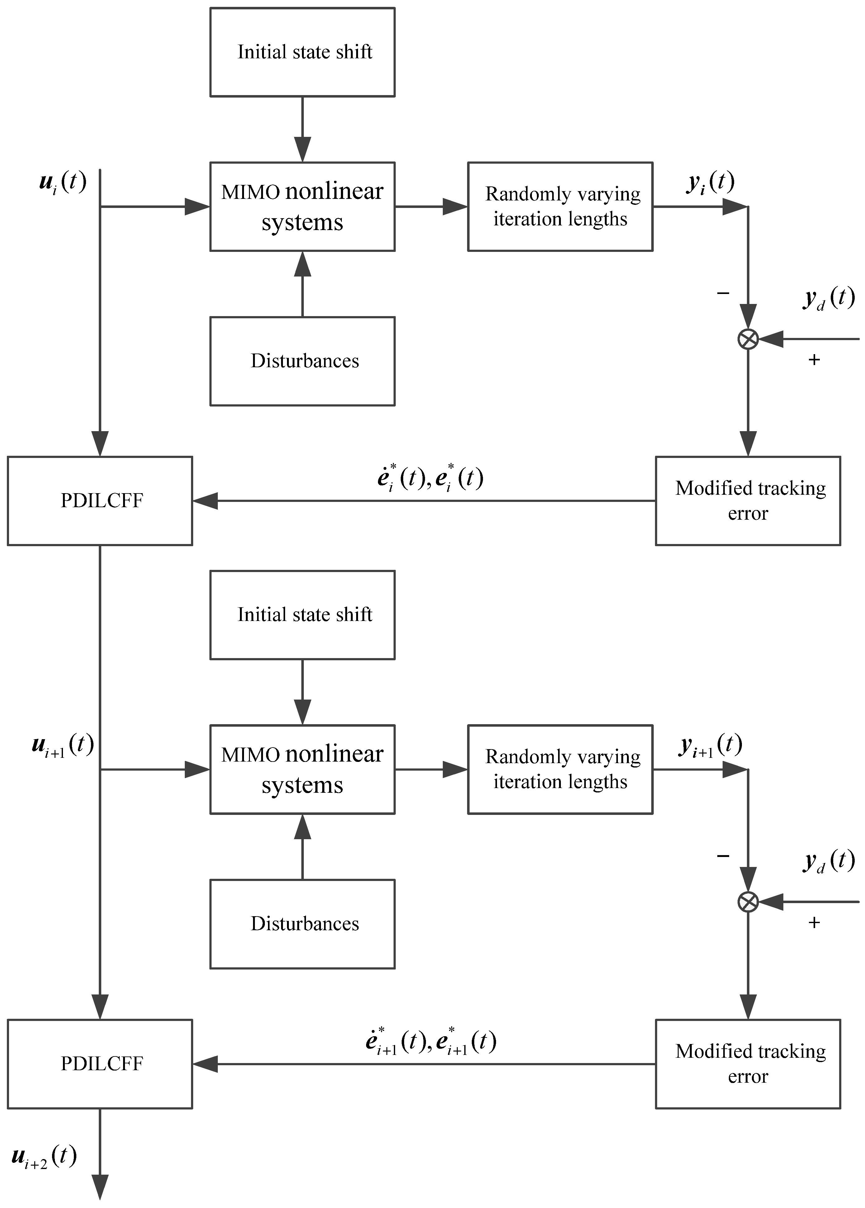
2. Problem Formulation

Consider the following MIMO continuous-time nonlinear system.

$$\begin{array}{l}{\stackrel{.}{\mathit{x}}}_i(t)=\mathit{f}({\mathit{x}}_i(t),t)+\mathit{B}{\mathit{u}}_i(t)+{\mathit{w}}_i(t)\\ {\mathit{y}}_i(t)=\mathit{C}{\mathit{x}}_i(t)+{\mathit{v}}_i(t)\end{array}$$

(1)

where i is the iteration index, $t\in [0,T_i]$ is time, and $T_i$ is the actual operation length. ${\mathit{x}}_i(t)\in {\mathit{R}}^n$, ${\mathit{u}}_i(t)\in {\mathit{R}}^r$, ${\mathit{y}}_i(t)\in {\mathit{R}}^m$. $\mathit{B}\in {\mathit{R}}^{n\times r}$, $\mathit{C}\in {\mathit{R}}^{m\times n}$. $w_i(t)\in {\mathit{R}}^n$ represents state disturbances, and ${\mathit{v}}_i(t)\in {\mathit{R}}^m$ represents measurement disturbances. $\Vert {\mathit{w}}_i(t)\Vert \le b_w$, $\Vert {\mathit{v}}_i(t)\Vert \le b_{v1}$, $\Vert {\stackrel{.}{\mathit{v}}}_i(t)\Vert \le b_{v2}$. $\mathit{f}(\cdot ,\cdot )$ is globally Lipschitz with respect to x. That is, $\Vert \mathit{f}(x_1,t)-\mathit{f}(x_2,t)\Vert \le k_f\Vert {\mathit{x}}_1(t)-{\mathit{x}}_2(t)\Vert ,t\in [0,T_i]$ where $k_f$ is the bounded Lipschitz constant.

Assume that for the desired output trajectory ${\mathit{y}}_d(t)$, $t\in [0,T_r]$ and initial state ${\mathit{x}}_d(0)$, there exists a unique input ${\mathit{u}}_d(t)$ such that

$$\begin{array}{l}{\stackrel{.}{\mathit{x}}}_d(t)=\mathit{f}({\mathit{x}}_d(t),t)+\mathit{B}{\mathit{u}}_d(t)\\ {\mathit{y}}_d(t)=\mathit{C}{\mathit{x}}_d(t)\end{array}$$

(2)

where $T_r$ is the desired operation length. The tracking error is defined as ${\mathit{e}}_i(t)={\mathit{y}}_d(t)-{\mathit{y}}_i(t)$.

3. Controller Design and Convergence Analysis

3.1. Randomly Varying Iteration Lengths

The primary difficulty in the design of the ILC system (1) is that the actual trial length is iteration varying, which is different from the desired operation length.

In practical applications, the actual operation length $T_i$ may be smaller or greater than the desired operation length $T_r$. Assume that the minimum iteration length is $T_{\min }$ and the maximal iteration length is $T_{\max }$. $T_i\in [T_{\min },T_{\max }]$ is a stochastic variable, which denotes the actual length at the i-th iteration.

For the first case, $T_i<t<T_r$, the system output data information is missing and cannot be utilized for control input updating. For the second case, $T_r<t<T_{\max }$, the system output data after the desired length are redundant and can be discarded because they have no use for learning control. In the second case, the full desired iteration length information is available. Hence, the second case can be considered a normal learning process.

Definition 1.

$E\{\mu \}$ is the mathematical expectation of the stochastic variable $\mu$. $P[T_i\le t]$ is the occurrence probability of the event $\mu \le t$.

Let the probability of a stochastic variable $T_i$ occurring at time t be q(t). Its probability distribution function is given as follows:

$${\Theta }_{T_i}(t)=P[T_i\le t]=\{\begin{array}{ll}0& t\in [0,T_{\min }]\\ q(t)& t\in [T_{\min },T_{\max }]\\ 1& t\in [T_{\max },\infty ]\end{array}$$

(3)

where $0\le q(t)\le 1$ is a known function.

To state the randomness of iteration length, a stochastic variable ${\upsilon }_i(t)\in R,t\in [0,T_{\max }]$ is given, which satisfies Bernoulli distribution by taking binary values of 0 and 1. The event ${\upsilon }_i(t)=1$ indicates that the learning process can operate at or after the time instant t with a probability of $p(t)$ satisfying $0<p(t)\le 1$. The event ${\upsilon }_i(t)=0$ indicates that the learning process cannot operate at the time instant k with a probability of $1-p(t)$. It is clear that the system output data are always available for any iteration in the time interval $[0,T_{\min }]$. Because the event ${\upsilon }_i(t)=1$, $t\in [0,T_{\min }]$ holds at any iteration, the probability is $p(t)=1$. For $t\in [T_{\min },T_{\max }]$, the event ${\upsilon }_i(t)=1$ indicates that the learning process stops at or after the time instant t, i.e., $T_i\ge t$.

Therefore, it yields

$$\begin{array}{l}P[{\upsilon }_i(t)=1]\\ =P[T_i\ge t]\\ =1-P[T_i<t]\\ =1-P[T_i<t]-P[T_i=t]\\ =1-P[T_i\le t]\\ =1-F_{T_i}(t)\end{array}$$

(4)

where $P[T_i=t]=0$.

Hence, we have

$$p(t)=1-{\Theta }_{T_i}(t)=\{\begin{array}{ll}1& t\in [0,T_{\min }]\\ 1-q(t)& t\in [T_{\min },T_{\max }]\\ 0& t\in [T_{\max },\infty ]\end{array}.$$

(5)

Because ${\upsilon }_i(t)$ satisfies Bernoulli distribution, the mathematical expectation of ${\upsilon }_i(t)$ is

$$E\{{\upsilon }_i(t)\}=1\cdot p(t)+0\cdot (1-p(t))=p(t).$$

(6)

Define the modified tracking error as ${\mathit{e}}_i^{\ast }(t)={\upsilon }_i(t){\mathit{e}}_i(t),t\in [0,T_r]$.

If $T_i<T_r$, we have

$${\mathit{e}}_i^{\ast }(t)=\{\begin{array}{ll}{\mathit{e}}_i(t)& t\in [0,T_i]\\ 0& t\in [T_i+1,T_r]\end{array}.$$

(7)

If $T_i\ge T_r$, it yields

$${\mathit{e}}_i^{\ast }(t)={\mathit{e}}_i(t)\hspace{1em}\hspace{1em}t\in [0,T_r].$$

(8)

3.2. Controller Design

According to the modified tracking error, the PD-type iterative learning control law with the forgetting factor (PDILCFF) is designed as follows.

$${\mathit{u}}_{i+1}(t)=(1-\beta ){\mathit{u}}_i(t)+\beta {\mathit{u}}_0(t)+\mathit{H}{\stackrel{.}{\mathit{e}}}_i^{\ast }(t)+\mathit{K}{\mathit{e}}_i^{\ast }(t)$$

(9)

where $0\le \beta <1$, $\beta$ is the forgetting factor. The initial input correction item $\beta u_0(t)$ can avoid the large oscillation of the iterative trajectory and accelerate the rate of convergence. $\mathit{H}$ and $\mathit{K}$ are the gain matrices of appropriate dimensions.

Figure 1 is a block diagram of the proposed PDILCFF method with randomly varying iteration lengths, the initial state shift and disturbances. In this paper, considering iteration-varying trial lengths, the proposed PDILCFF algorithm is closely related to symmetry. Symmetry can provide prior information about the system structure and characteristics of the proposed PDILCFF method, which is helpful for designing more efficient control algorithms. On the other hand, the proposed PDILCFF method exploits system symmetries in different intervals through iterative processes to achieve accurate control and performance optimization of MIMO unknown nonlinear systems.

3.3. Convergence Analysis

Definition 2.

Define the $\lambda$ norm for a function $\mathit{F}:[0,T]\to {\mathit{R}}^n$ by ${\Vert \mathit{F}(\cdot )\Vert }_{\lambda }=\underset{t\in [0,T_i]}{\sup }{e}^{-\lambda t}\Vert \mathit{F}(\cdot )\Vert$.

Assumption 1.

The initial state error is bounded, i.e., $\Vert {\mathit{x}}_d(0)-{\mathit{x}}_i(0)\Vert \le b_{x0}$, where $b_{x0}$ is a positive constant.

Lemma 1.

If the sequence $c_p\in R$, satisfies $\left|c_{p+1}\right|\le \alpha \left|c_p\right|+\epsilon ,0\le \alpha <1$, where $\epsilon \in R$, $p\in Z^{+}$, the following inequation is held.

$$\underset{p\to \infty }{\lim \sup }\left|c_p\right|\le {\displaystyle \frac{1}{1-\alpha }}\epsilon .$$

Proof: 

According to $\left|c_{p+1}\right|\le \alpha \left|c_p\right|+\epsilon$, we have

$$\begin{array}{l}\left|c_1\right|\le \alpha \left|c_0\right|+\epsilon \\ \left|c_2\right|\le {\alpha }^2\left|c_0\right|+(1+\alpha )\epsilon \\ \hspace{1em}⋮\\ \left|c_p\right|\le {\alpha }^p\left|c_0\right|+{\displaystyle \sum _{j=1}^p{\alpha }^{p-j}\epsilon }={\alpha }^p\left|c_0\right|+{\displaystyle \frac{1-{\alpha }^p}{1-\alpha }}\epsilon \end{array}.$$

Due to $0\le \alpha <1$, we obtain $\left|c_p\right|\le \left|c_0\right|+{\displaystyle \frac{1}{1-\alpha }}\epsilon$.

Therefore, when $p\to \infty$, it leads to $\underset{p\to \infty }{\lim \sup }\left|c_p\right|\le {\displaystyle \frac{1}{1-\alpha }}\epsilon$. □

Lemma 2 (Gronwall’s lemma).

 Let $x(t)$ and $y(t)$ be real-valued continuous functions defined on the interval [0, T], $a\ge 0$. If $x(t)\le c+{\displaystyle {\int }_0^t(ax(\tau )+by(\tau ))d\tau }$, then $x(t)\le c+{\displaystyle {\int }_0^t(ax(\tau )+by(\tau ))d\tau }$.

Theorem 1.

For nonlinear system (1), if $\Vert (1-\beta )\mathit{I}-\mathit{HCB}\Vert \le \alpha <1$ and assumption 1 are satisfied, the PDILCFF algorithm (9) can ensure that the tracking error is uniformly ultimately bounded as the iteration number i approaches infinity.

Proof: 

The proof consists of two parts. Part A demonstrates that the error between ${\mathit{u}}_d(t)$ and ${\mathit{u}}_i(t)$ is bounded. Part B shows that the state and output errors are bounded.

Part A:

According to (2) and (9), we have

$$\begin{array}{l}{\mathit{u}}_d-{\mathit{u}}_{i+1}\\ ={\mathit{u}}_d-[(1-\beta ){\mathit{u}}_i+\beta {\mathit{u}}_0+\mathit{H}{\upsilon }_i({\stackrel{.}{\mathit{y}}}_d-{\stackrel{.}{\mathit{y}}}_i)+\mathit{K}{\upsilon }_i({\mathit{y}}_d-{\mathit{y}}_i)]\\ =(1-\beta )({\mathit{u}}_d-{\mathit{u}}_i)+\beta ({\mathit{u}}_d-{\mathit{u}}_0)\\ \hspace{1em}-\mathit{H}{\upsilon }_i[\mathit{C}({\mathit{f}}_d+\mathit{B}{\mathit{u}}_d)-\mathit{C}({\mathit{f}}_i+\mathit{B}{\mathit{u}}_i+{\mathit{w}}_i)-{\stackrel{.}{\mathit{v}}}_i]\\ \hspace{1em}-\mathit{K}{\upsilon }_i(\mathit{C}{\mathit{x}}_d-\mathit{C}{\mathit{x}}_i-{\mathit{v}}_i)\\ =[(1-\beta )\mathit{I}-\mathit{H}{\upsilon }_i\mathit{CB}]({\mathit{u}}_d-{\mathit{u}}_i)+\beta ({\mathit{u}}_d-{\mathit{u}}_0)\\ \hspace{1em}-\mathit{H}{\upsilon }_i\mathit{C}[({\mathit{f}}_d+\mathit{B}{\mathit{u}}_d)-({\mathit{f}}_i+\mathit{B}{\mathit{u}}_d+{\mathit{w}}_i)]+\mathit{H}{\upsilon }_i{\stackrel{.}{\mathit{v}}}_i\\ \hspace{1em}-\mathit{K}{\upsilon }_i\mathit{C}({\mathit{x}}_d-{\mathit{x}}_i)+\mathit{K}{\upsilon }_i{\mathit{v}}_i\end{array}.$$

(10)

Taking the norm of both sides of (10), we have

$$\begin{array}{l}\Vert {\mathit{u}}_d-{\mathit{u}}_{i+1}\Vert \\ \le \Vert (1-\beta )\mathit{I}-\mathit{H}{\upsilon }_i\mathit{CB}\Vert \Vert {\mathit{u}}_d-{\mathit{u}}_i\Vert +\beta \Vert {\mathit{u}}_d-{\mathit{u}}_0\Vert \\ \hspace{1em}+\Vert \mathit{H}{\upsilon }_i\mathit{C}\Vert \left[k_f\Vert {\mathit{x}}_d-{\mathit{x}}_i\Vert \right]+\Vert \mathit{H}{\upsilon }_i\mathit{C}\Vert \Vert {\mathit{w}}_i\Vert +\Vert \mathit{H}{\upsilon }_i\Vert \Vert {\stackrel{.}{\mathit{v}}}_i\Vert \\ \hspace{1em}+\Vert \mathit{K}{\upsilon }_i\mathit{C}\Vert \Vert {\mathit{x}}_d-{\mathit{x}}_i\Vert +\Vert \mathit{K}{\upsilon }_i\Vert \Vert {\mathit{v}}_i\Vert \\ \le \Vert (1-\beta )\mathit{I}-\mathit{H}{\upsilon }_i\mathit{CB}\Vert \Vert {\mathit{u}}_d-{\mathit{u}}_i\Vert +\beta \Vert {\mathit{u}}_d-{\mathit{u}}_0\Vert \\ \hspace{1em}+\left(\Vert \mathit{H}{\upsilon }_i\mathit{C}\Vert k_f+\Vert \mathit{K}{\upsilon }_i\mathit{C}\Vert \right)\Vert {\mathit{x}}_d-{\mathit{x}}_i\Vert \\ \hspace{1em}+\Vert \mathit{H}{\upsilon }_i\mathit{C}\Vert b_w+\Vert \mathit{H}{\upsilon }_i\Vert b_{v2}+\Vert \mathit{K}{\upsilon }_i\Vert b_{v1}\end{array}.$$

(11)

According to system (1) and the globally Lipschitz condition for $\mathit{f}(\cdot ,\cdot )$, the following can be obtained:

$$\begin{array}{l}\Vert {\mathit{x}}_d-{\mathit{x}}_i\Vert \\ =\Vert {\mathit{x}}_d(0)-{\mathit{x}}_i(0)+{\displaystyle {\int }_0^t\left(({\mathit{f}}_d+\mathit{B}{\mathit{u}}_d)-({\mathit{f}}_i+\mathit{B}{\mathit{u}}_i+{\mathit{w}}_i)\right)d\tau }\Vert \\ =\Vert {\mathit{x}}_d(0)-{\mathit{x}}_i(0)+{\displaystyle {\int }_0^t\left({\mathit{f}}_d-{\mathit{f}}_i+\mathit{B}({\mathit{u}}_d-{\mathit{u}}_i)-{\mathit{w}}_i\right)d\tau }\Vert \\ \le \Vert {\mathit{x}}_d(0)-{\mathit{x}}_i(0)\Vert +{\displaystyle {\int }_0^t\left(\Vert {\mathit{f}}_d-{\mathit{f}}_i\Vert +\Vert \mathit{B}\Vert \Vert {\mathit{u}}_d-{\mathit{u}}_i\Vert +\Vert {\mathit{w}}_i\Vert \right)d\tau }\\ \le \Vert {\mathit{x}}_d(0)-{\mathit{x}}_i(0)\Vert +{\displaystyle {\int }_0^t\left(k_f\Vert {\mathit{x}}_d-{\mathit{x}}_i\Vert +b_B\Vert {\mathit{u}}_d-{\mathit{u}}_i\Vert +b_w\right)d\tau }\end{array}$$

(12)

where $\Vert \mathit{B}\Vert \le b_B$.

Define $\Delta {\mathit{x}}_i={\mathit{x}}_d-{\mathit{x}}_i$ and $\Delta {\mathit{u}}_i={\mathit{u}}_d-{\mathit{u}}_i$. According to Gronwall’s lemma, we have

$$\begin{array}{l}\Vert \Delta {\mathit{x}}_i\Vert \\ \le \Vert \Delta {\mathit{x}}_i(0)\Vert +{\displaystyle {\int }_0^t\left(k_f\Vert \Delta {\mathit{x}}_i\Vert +b_B\Vert \Delta {\mathit{u}}_i\Vert +b_w\right)d\tau }\\ \le \Vert \Delta {\mathit{x}}_i(0)\Vert e^{k_{f}t}+{\displaystyle {\int }_0^t{e}^{k_f(t-\tau )}\left(b_B\Vert \Delta {\mathit{u}}_i(\tau )\Vert +b_w\right)d\tau }\\ =\Vert \Delta {\mathit{x}}_i(0)\Vert e^{k_{f}t}+b_B{\displaystyle {\int }_0^t{e}^{k_f(t-\tau )}\Vert \Delta {\mathit{u}}_i(\tau )\Vert d\tau }+b_w{\displaystyle {\int }_0^t{e}^{k_f(t-\tau )}d\tau }\end{array}.$$

(13)

Substituting (13) into (11) yields the following:

$$\begin{array}{l}\Vert \Delta {\mathit{u}}_{i+1}\Vert \\ \le \Vert (1-\beta )\mathit{I}-\mathit{H}{\upsilon }_i\mathit{CB}\Vert \Vert \Delta {\mathit{u}}_i\Vert +\beta \Vert \Delta {\mathit{u}}_0\Vert \\ \hspace{1em}+\left(\Vert \mathit{H}{\upsilon }_i\mathit{C}\Vert k_f+\Vert \mathit{K}{\upsilon }_i\mathit{C}\Vert \right)\Vert \Delta {\mathit{x}}_i\Vert \\ \hspace{1em}+\Vert \mathit{H}{\upsilon }_i\mathit{C}\Vert b_w+\Vert \mathit{H}{\upsilon }_i\Vert b_{v2}+\Vert \mathit{K}{\upsilon }_i\Vert b_{v1}\\ \le \Vert (1-\beta )\mathit{I}-\mathit{H}{\upsilon }_i\mathit{CB}\Vert \Vert \Delta {\mathit{u}}_i\Vert +\beta \Vert \Delta {\mathit{u}}_0\Vert \\ \hspace{1em}+\left(\Vert \mathit{H}{\upsilon }_i\mathit{C}\Vert k_f+\Vert \mathit{K}{\upsilon }_i\mathit{C}\Vert \right)\\ \times \left(\Vert \Delta {\mathit{x}}_i(0)\Vert e^{k_{f}t}+b_B{\displaystyle {\int }_0^t{e}^{k_f(t-\tau )}\Vert \Delta {\mathit{u}}_i(\tau )\Vert d\tau }+b_w{\displaystyle {\int }_0^t{e}^{k_f(t-\tau )}d\tau }\right)\\ \hspace{1em}+\Vert \mathit{H}{\upsilon }_i\mathit{C}\Vert b_w+\Vert \mathit{H}{\upsilon }_i\Vert b_{v2}+\Vert \mathit{K}{\upsilon }_i\Vert b_{v1}\\ =\Vert (1-\beta )\mathit{I}-\mathit{H}{\upsilon }_i\mathit{CB}\Vert \Vert \Delta {\mathit{u}}_i\Vert +\beta \Vert \Delta {\mathit{u}}_0\Vert \\ \hspace{1em}+\left(\Vert \mathit{H}{\upsilon }_i\mathit{C}\Vert k_f+\Vert \mathit{H}{\upsilon }_i\mathit{C}\Vert \right)\Vert \Delta {\mathit{x}}_i(0)\Vert e^{k_{f}t}\\ \hspace{1em}+\left(\Vert \mathit{H}{\upsilon }_i\mathit{C}\Vert k_f+\Vert \mathit{H}{\upsilon }_i\mathit{C}\Vert \right)b_B{\displaystyle {\int }_0^t{e}^{k_f(t-\tau )}\Vert \Delta {\mathit{u}}_i(\tau )\Vert d\tau }\\ \hspace{1em}+\left(\Vert \mathit{H}{\upsilon }_i\mathit{C}\Vert k_f+\Vert \mathit{H}{\upsilon }_i\mathit{C}\Vert \right)b_w{\displaystyle {\int }_0^t{e}^{k_f(t-\tau )}d\tau }\\ \hspace{1em}+\Vert \mathit{H}{\upsilon }_i\mathit{C}\Vert b_w+\Vert \mathit{H}{\upsilon }_i\Vert b_{v2}+\Vert \mathit{K}{\upsilon }_i\Vert b_{v1}\end{array}.$$

(14)

Multiplying (14) by $e^{-\lambda t}$, leads to

$$\begin{array}{l}{e}^{-\lambda t}\Vert \Delta {\mathit{u}}_{i+1}\Vert \\ \le \Vert (1-\beta )\mathit{I}-\mathit{H}{\upsilon }_i\mathit{CB}\Vert e^{-\lambda t}\Vert \Delta {\mathit{u}}_i\Vert +\beta e^{-\lambda t}\Vert \Delta {\mathit{u}}_0\Vert \\ \hspace{1em}+\left(\Vert \mathit{H}{\upsilon }_i\mathit{C}\Vert k_f+\Vert \mathit{K}{\upsilon }_i\mathit{C}\Vert \right)\Vert \Delta {\mathit{x}}_i(0)\Vert e^{(k_f-\lambda )t}\\ \hspace{1em}+\left(\Vert \mathit{H}{\upsilon }_i\mathit{C}\Vert k_f+\Vert \mathit{K}{\upsilon }_i\mathit{C}\Vert \right)b_B{\displaystyle {\int }_0^t{e}^{-\lambda \tau }{e}^{(k_f-\lambda )(t-\tau )}\Vert \Delta {\mathit{u}}_i(\tau )\Vert d\tau }\\ \hspace{1em}+\left(\Vert \mathit{H}{\upsilon }_i\mathit{C}\Vert k_f+\Vert \mathit{K}{\upsilon }_i\mathit{C}\Vert \right)b_w{\displaystyle {\int }_0^t{e}^{-\lambda \tau }{e}^{(k_f-\lambda )(t-\tau )}d\tau }\\ \hspace{1em}+\Vert \mathit{H}{\upsilon }_i\mathit{C}\Vert b_w{e}^{-\lambda t}+\Vert \mathit{H}{\upsilon }_i\Vert b_{v2}{e}^{-\lambda t}+\Vert \mathit{K}{\upsilon }_i\Vert b_{v1}{e}^{-\lambda t}\end{array}.$$

(15)

Therefore, we obtain

$$\begin{array}{l}{\Vert \Delta {\mathit{u}}_{i+1}\Vert }_{\lambda }\\ \le \Vert (1-\beta )\mathit{I}-\mathit{H}{\upsilon }_i\mathit{CB}\Vert {\Vert \Delta {\mathit{u}}_i\Vert }_{\lambda }\\ \hspace{1em}+\left(\Vert \mathit{H}{\upsilon }_i\mathit{C}\Vert k_f+\Vert \mathit{K}{\upsilon }_i\mathit{C}\Vert \right)b_B{\displaystyle {\int }_0^t{e}^{(k_f-\lambda )(t-\tau )}d\tau }{\Vert \Delta {\mathit{u}}_i\Vert }_{\lambda }\\ \hspace{1em}+\beta {\Vert \Delta {\mathit{u}}_0\Vert }_{\lambda }+\left(\Vert \mathit{H}{\upsilon }_i\mathit{C}\Vert k_f+\Vert \mathit{K}{\upsilon }_i\mathit{C}\Vert \right)\Vert \Delta {\mathit{x}}_i(0)\Vert e^{(k_f-\lambda )t}\\ \hspace{1em}+\left(\Vert \mathit{H}{\upsilon }_i\mathit{C}\Vert k_f+\Vert \mathit{K}{\upsilon }_i\mathit{C}\Vert \right)b_w{\displaystyle {\int }_0^t{e}^{(k_f-\lambda )(t-\tau )}d\tau }\\ \hspace{1em}+\Vert \mathit{H}{\upsilon }_i\mathit{C}\Vert b_w+\Vert \mathit{H}{\upsilon }_i\Vert b_{v2}+\Vert \mathit{K}{\upsilon }_i\Vert b_{v1}\end{array}.$$

(16)

Taking mathematical expectation of both sides of (16) and noting that ${\upsilon }_i$ is the only stochastic variable leads to

$$\begin{array}{l}{\Vert \Delta {\mathit{u}}_{i+1}\Vert }_{\lambda }\\ \le E\{\Vert (1-\beta )\mathit{I}-\mathit{H}{\upsilon }_i\mathit{CB}\Vert \}{\Vert \Delta {\mathit{u}}_i\Vert }_{\lambda }\\ \hspace{1em}+E\{\left(\Vert \mathit{H}{\upsilon }_i\mathit{C}\Vert k_f+\Vert \mathit{K}{\upsilon }_i\mathit{C}\Vert \right)\}{b}_B{\displaystyle {\int }_0^t{e}^{(k_f-\lambda )(t-\tau )}d\tau }{\Vert \Delta {\mathit{u}}_i\Vert }_{\lambda }\\ \hspace{1em}+\beta {\Vert \Delta {\mathit{u}}_0\Vert }_{\lambda }+E\{\left(\Vert \mathit{H}{\upsilon }_i\mathit{C}\Vert k_f+\Vert \mathit{K}{\upsilon }_i\mathit{C}\Vert \right)\}\Vert \Delta {\mathit{x}}_i(0)\Vert e^{(k_f-\lambda )t}\\ \hspace{1em}+E\{\left(\Vert \mathit{H}{\upsilon }_i\mathit{C}\Vert k_f+\Vert \mathit{K}{\upsilon }_i\mathit{C}\Vert \right)\}{b}_w{\displaystyle {\int }_0^t{e}^{(k_f-\lambda )(t-\tau )}d\tau }\\ \hspace{1em}+E\{\Vert \mathit{H}{\upsilon }_i\mathit{C}\Vert \}{b}_w+E\{\Vert \mathit{H}{\upsilon }_i\Vert \}{b}_{v2}+E\{\Vert \mathit{K}{\upsilon }_i\Vert \}{b}_{v1}\\ =\Vert (1-\beta )\mathit{I}-\mathit{H}p\mathit{CB}\Vert {\Vert \Delta {\mathit{u}}_i\Vert }_{\lambda }\\ \hspace{1em}+\left(\Vert \mathit{H}p\mathit{C}\Vert k_f+\Vert \mathit{K}p\mathit{C}\Vert \right)b_B{\displaystyle {\int }_0^t{e}^{(k_f-\lambda )(t-\tau )}d\tau }{\Vert \Delta {\mathit{u}}_i\Vert }_{\lambda }\\ \hspace{1em}+\beta {\Vert \Delta {\mathit{u}}_0\Vert }_{\lambda }+\left(\Vert \mathit{H}p\mathit{C}\Vert k_f+\Vert \mathit{K}p\mathit{C}\Vert \right)\Vert \Delta {\mathit{x}}_i(0)\Vert e^{(k_f-\lambda )t}\\ \hspace{1em}+\left(\Vert \mathit{H}p\mathit{C}\Vert k_f+\Vert \mathit{K}p\mathit{C}\Vert \right)b_w{\displaystyle {\int }_0^t{e}^{(k_f-\lambda )(t-\tau )}d\tau }\\ \hspace{1em}+\Vert \mathit{H}p\mathit{C}\Vert b_w+\Vert \mathit{H}p\Vert b_{v2}+\Vert \mathit{K}p\Vert b_{v1}\\ ={\mathit{ħ}}_1{\Vert \Delta {\mathit{u}}_i\Vert }_{\lambda }+{\mathit{ħ}}_2{b}_B{\displaystyle {\int }_0^t{e}^{(k_f-\lambda )(t-\tau )}d\tau }{\Vert \Delta {\mathit{u}}_i\Vert }_{\lambda }\\ \hspace{1em}+\beta {\Vert \Delta {\mathit{u}}_0\Vert }_{\lambda }+{\mathit{ħ}}_2\Vert \Delta {\mathit{x}}_i(0)\Vert e^{(k_f-\lambda )t}+{\mathit{ħ}}_3{b}_w{\displaystyle {\int }_0^t{e}^{(k_f-\lambda )(t-\tau )}d\tau }\\ \hspace{1em}+\Vert \mathit{H}p\mathit{C}\Vert b_w+\Vert \mathit{H}p\Vert b_{v2}+\Vert \mathit{K}p\Vert b_{v1}\end{array}$$

(17)

where ${\mathit{ħ}}_1=(1-\beta )\mathit{I}-\mathit{H}p\mathit{CB}$, ${\mathit{ħ}}_2=\Vert \mathit{H}p\mathit{C}\Vert k_f+\Vert \mathit{K}p\mathit{C}\Vert$, ${\mathit{ħ}}_3=\Vert \mathit{H}p\mathit{C}\Vert k_f+\Vert \mathit{K}p\mathit{C}\Vert$.

Define $\mathit{ħ}=\max \{{\mathit{ħ}}_2{b}_B,k_f\}$. Assume that $\lambda >\mathit{ħ}$. It yields

$$\begin{array}{l}{\Vert \Delta {\mathit{u}}_{i+1}\Vert }_{\lambda }\\ \le {\mathit{ħ}}_1{\Vert \Delta {\mathit{u}}_i\Vert }_{\lambda }+\mathit{ħ}{\displaystyle {\int }_0^t{e}^{(\mathit{ħ}-\lambda )(t-\tau )}d\tau }{\Vert \Delta {\mathit{u}}_i\Vert }_{\lambda }+\beta {\Vert \Delta {\mathit{u}}_0\Vert }_{\lambda }+{\mathit{ħ}}_2\Vert \Delta {\mathit{x}}_i(0)\Vert e^{(k_f-\lambda )t}\\ \hspace{1em}+{\mathit{ħ}}_3{b}_w{\displaystyle {\int }_0^t{e}^{(k_f-\lambda )(t-\tau )}d\tau }+\Vert \mathit{H}p\mathit{C}\Vert b_w+\Vert \mathit{H}p\Vert b_{v2}+\Vert \mathit{K}p\Vert b_{v1}\\ \le \left({\mathit{ħ}}_1+{\displaystyle \frac{\mathit{ħ}}{\lambda -\mathit{ħ}}}(1-e^{(\mathit{ħ}-\lambda )T_i})\right){\Vert \Delta {\mathit{u}}_i\Vert }_{\lambda }\\ \hspace{1em}+\beta {\Vert \Delta {\mathit{u}}_0\Vert }_{\lambda }+{\mathit{ħ}}_2\Vert \Delta {\mathit{x}}_i(0)\Vert +{\displaystyle \frac{{\mathit{ħ}}_3{b}_w}{1-k_f}}(1-e^{(k_f-\lambda )T_i})\\ \hspace{1em}+\Vert \mathit{H}p\mathit{C}\Vert b_w+\Vert \mathit{H}p\Vert b_{v2}+\Vert \mathit{K}p\Vert b_{v1}\\ =\left({\mathit{ħ}}_1+{\displaystyle \frac{\mathit{ħ}}{\lambda -\mathit{ħ}}}(1-e^{(\mathit{ħ}-\lambda )T_i})\right){\Vert \Delta {\mathit{u}}_i\Vert }_{\lambda }+\beta {\Vert \Delta {\mathit{u}}_0\Vert }_{\lambda }+{\mathit{ħ}}_2\Vert \Delta {\mathit{x}}_i(0)\Vert \\ \hspace{1em}+\left(\Vert \mathit{H}p\mathit{C}\Vert +{\displaystyle \frac{{\mathit{ħ}}_3}{1-k_f}}(1-e^{(k_f-\lambda )T_i})\right)b_w+\Vert \mathit{H}p\Vert b_{v2}+\Vert \mathit{K}p\Vert b_{v1}\end{array}$$

(18)

Defining ${\mathit{ħ}}_3={\mathit{ħ}}_1+{\displaystyle \frac{\mathit{ħ}}{\lambda -\mathit{ħ}}}(1-e^{(\mathit{ħ}-\lambda )T_i})$ and ${\mathit{ħ}}_4=\Vert \mathit{H}p\mathit{C}\Vert +{\displaystyle \frac{{\mathit{ħ}}_3}{1-k_f}}(1-e^{(k_f-\lambda )T_i})$, we obtain

$$\begin{array}{l}{\Vert \Delta {\mathit{u}}_{i+1}\Vert }_{\lambda }\\ \le {\mathit{ħ}}_3{\Vert \Delta {\mathit{u}}_i\Vert }_{\lambda }+\beta {\Vert \Delta {\mathit{u}}_0\Vert }_{\lambda }+{\mathit{ħ}}_2\Vert \Delta {\mathit{x}}_i(0)\Vert \\ \hspace{1em}+{\mathit{ħ}}_4{b}_w+\Vert \mathit{H}p\Vert b_{v2}+\Vert \mathit{K}p\Vert b_{v1}\end{array}.$$

(19)

Further, it yields

$${\Vert \Delta {\mathit{u}}_{i+1}\Vert }_{\lambda }\le {\mathit{ħ}}_3{\Vert \Delta {\mathit{u}}_i\Vert }_{\lambda }+\sigma$$

(20)

where $\sigma =\beta {\Vert \Delta {\mathit{u}}_0\Vert }_{\lambda }+{\mathit{ħ}}_2\Vert \Delta {\mathit{x}}_i(0)\Vert +{\mathit{ħ}}_4{b}_w+\Vert \mathit{H}p\Vert b_{v2}+\Vert \mathit{K}p\Vert b_{v1}$, which includes the norm bounds of the initial state errors, state disturbances, and bias contribution.

Due to $0<p\le 1$, we have ${\mathit{ħ}}_1<1$. There must exist a sufficiently large $\lambda$ such that $\lambda >\mathit{ħ}$. Therefore, we have ${\mathit{ħ}}_3<1$. In terms of (20) and lemma 1, we obtain

$$\underset{i\to \infty }{\lim }\sup {\Vert \Delta {\mathit{u}}_{i+1}\Vert }_{\lambda }\le {\displaystyle \frac{1}{1-{\mathit{ħ}}_3}}\sigma .$$

(21)

Part B:

According to (13), we obtain

$$\begin{array}{l}{\Vert \Delta {\mathit{x}}_i\Vert }_{\lambda }\\ \le \Vert \Delta {\mathit{x}}_i(0)\Vert +{\displaystyle {\int }_0^t{e}^{k_f(t-\tau )}\left(b_B\Vert \Delta {\mathit{u}}_i(\tau )\Vert +b_w\right)d\tau }\\ \le \Vert \Delta {\mathit{x}}_i(0)\Vert +{\displaystyle {\int }_0^t{e}^{(k_f-\lambda )(t-\tau )}\left(b_B{\Vert \Delta {\mathit{u}}_i\Vert }_{\lambda }+b_w\right)d\tau }\\ \le b_{x0}+{\displaystyle \frac{1}{\lambda -k_f}}(1-e^{(k_f-\lambda )T_i})\left(b_B{\Vert \Delta {\mathit{u}}_i\Vert }_{\lambda }+b_w\right)\end{array}.$$

(22)

From (21) and (22), we obtain

$$\underset{i\to \infty }{\lim }\sup {\Vert \Delta {\mathit{x}}_i\Vert }_{\lambda }\le b_{x0}+{\displaystyle \frac{1}{\lambda -k_f}}(1-e^{(k_f-\lambda )T_i})\left({\displaystyle \frac{b_B}{1-{\mathit{ħ}}_3}}\sigma +b_w\right).$$

(23)

Because ${\mathit{e}}_i={\mathit{y}}_d-{\mathit{y}}_i=\mathit{C}\Delta {\mathit{x}}_i(t)-{\mathit{v}}_i(t)$, we have

$${\Vert {\mathit{e}}_i\Vert }_{\lambda }\le \Vert \mathit{C}\Vert \Vert \Delta {\mathit{x}}_i(t)\Vert +\Vert {\mathit{v}}_i(t)\Vert \le c{\Vert \Delta {\mathit{x}}_i\Vert }_{\lambda }+b_{v1}$$

(24)

where $\Vert \mathit{C}\Vert \le c$, c is a constant.

According to (24), ${\Vert {\mathit{e}}_i\Vert }_{\lambda }$ is bounded.

According to (21), (23) and (24), it is clear that the initial state error, state disturbance and bias term influence the errors. If $\sigma =0$ $b_{x0}=0$, $b_w=0$ and $b_{v1}=0$, the tracking errors can converge to zero.

The proof of Theorem 1 is complete. □

Remark 1.

In this paper, the forgetting factor can enable the system to maintain stability and good performance when factors such as external interference and initial state shifts occur. When the system is disturbed, the forgetting factor enables the algorithm to remove the influence of the interference on the information of past iterations more quickly and readjust the control input to deal with the new situation, thereby enhancing the robustness and anti-interference ability of the system.

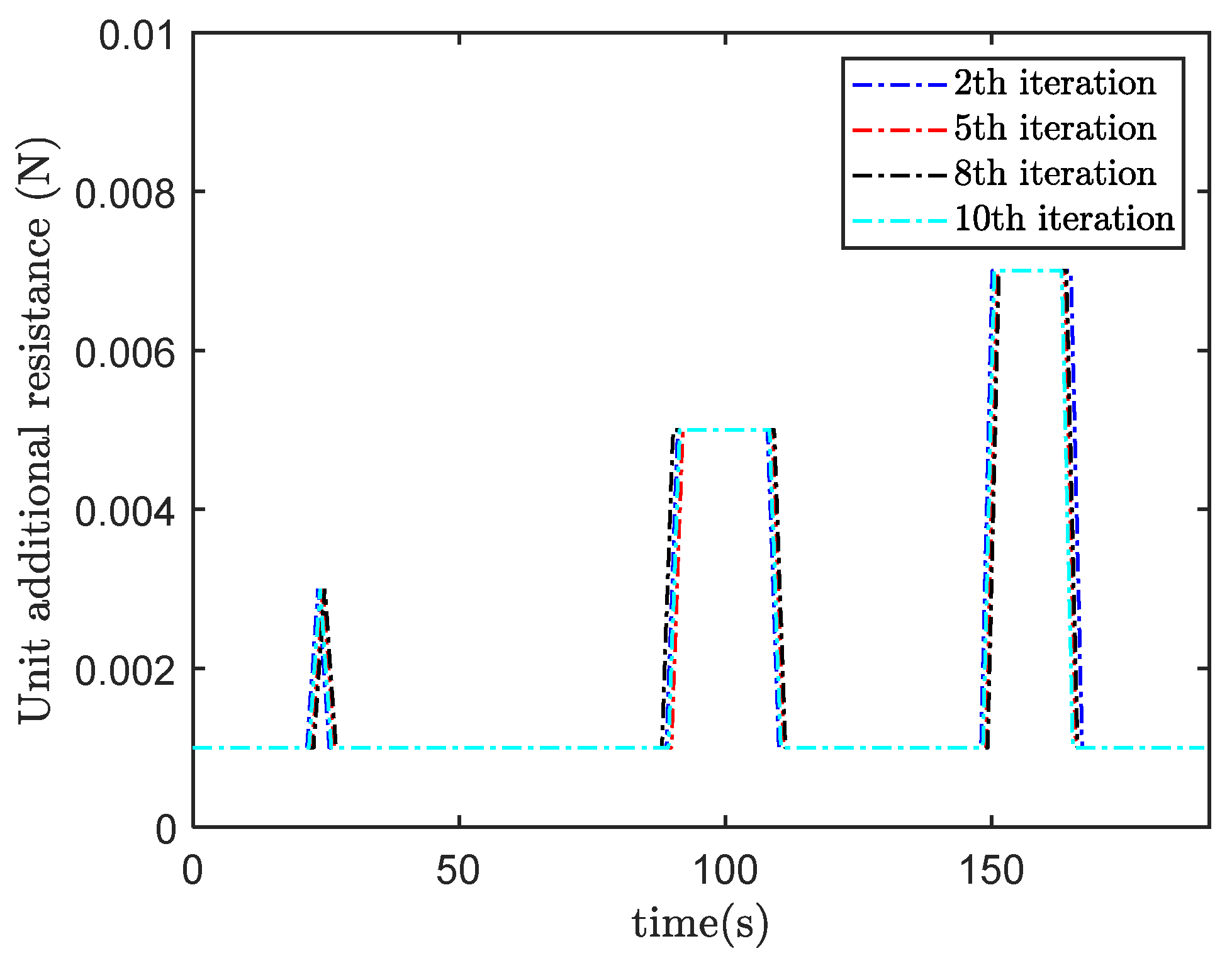
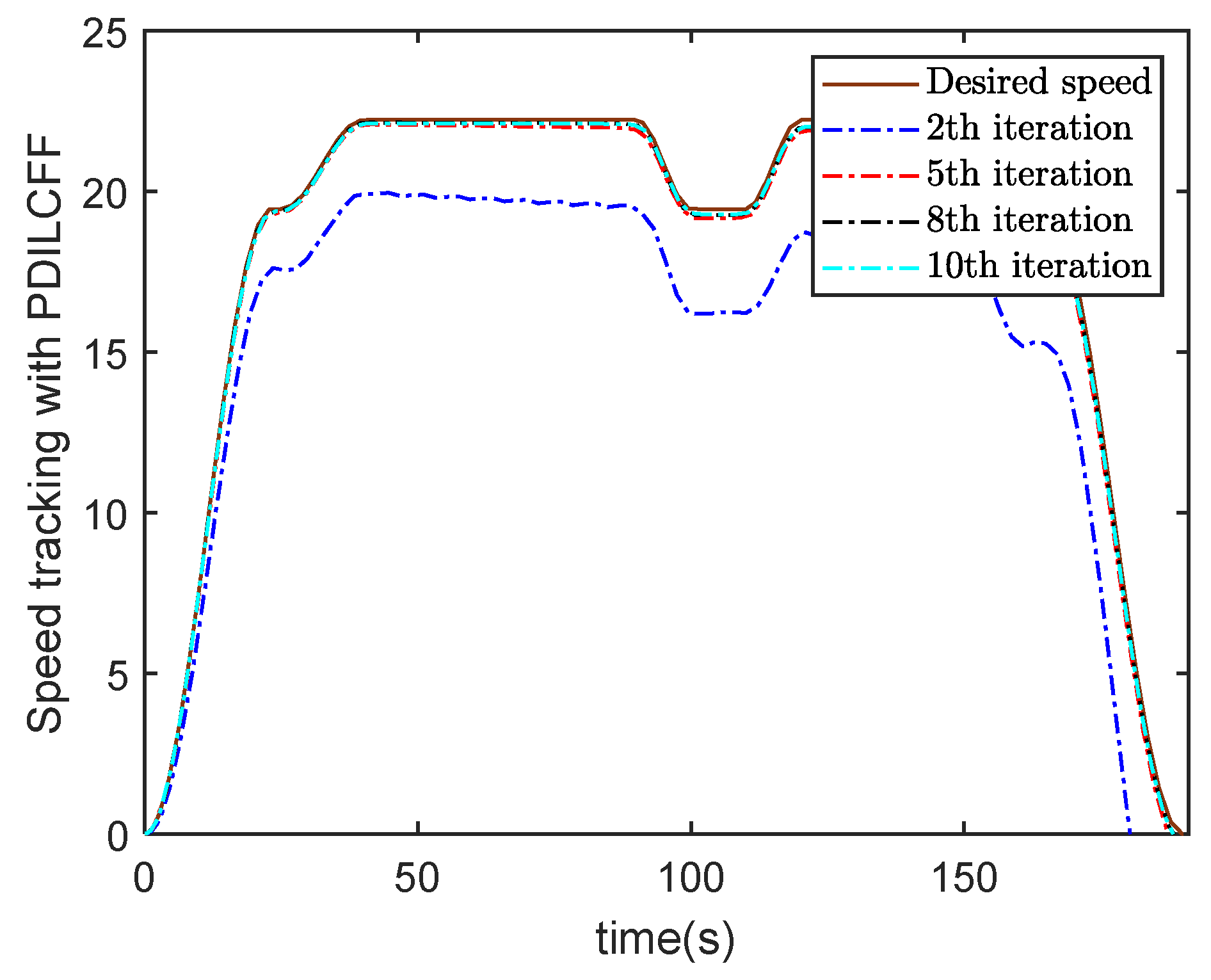
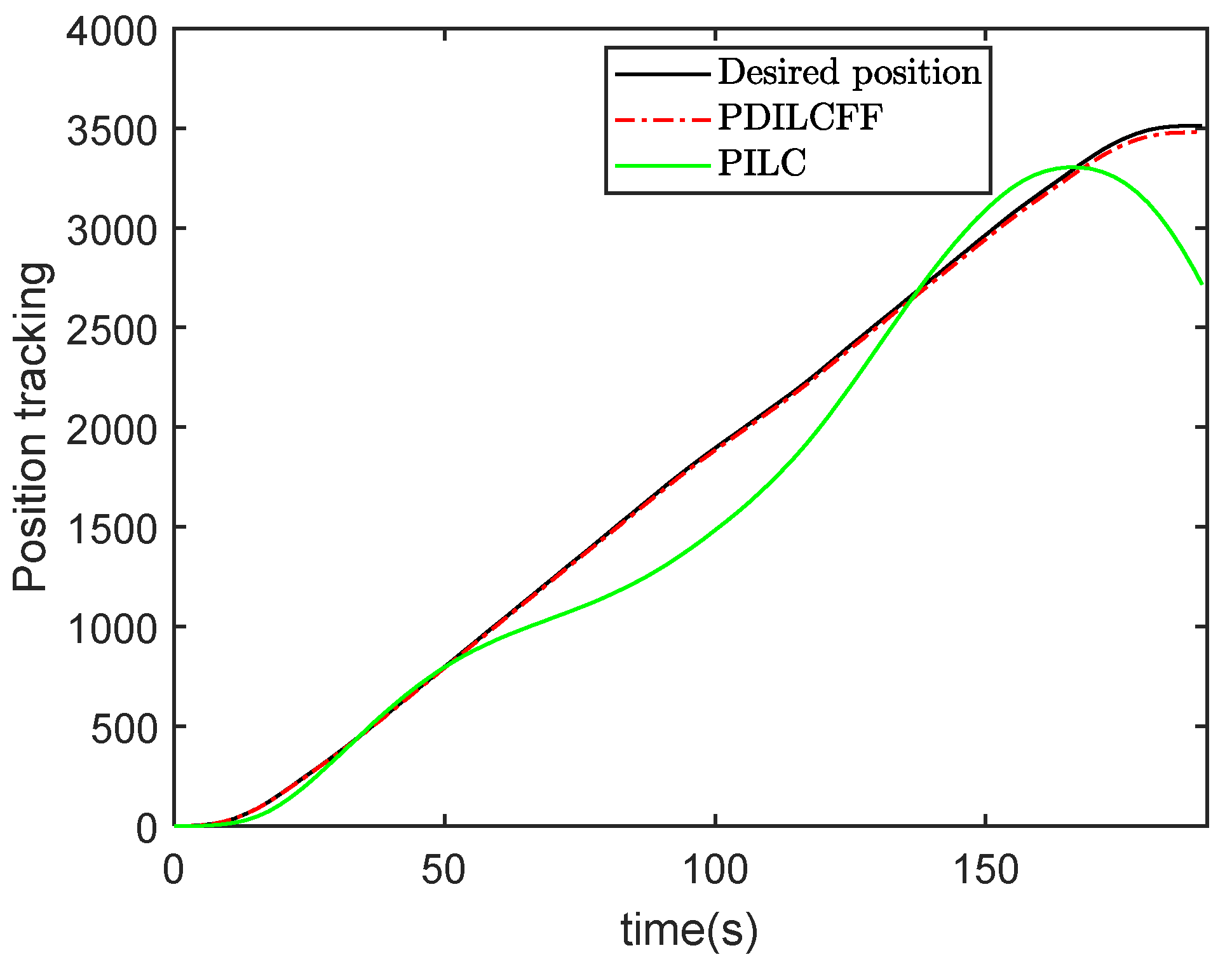
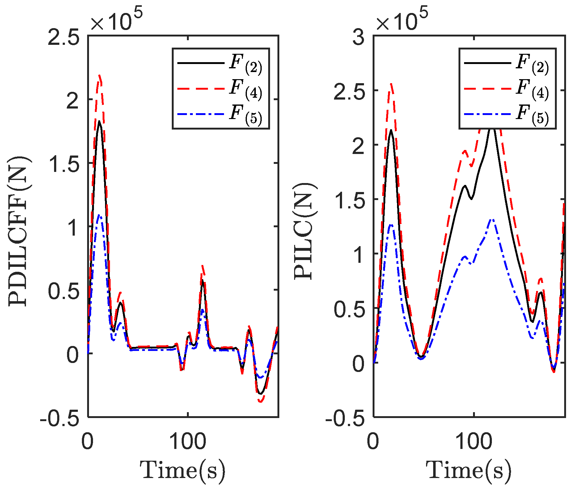
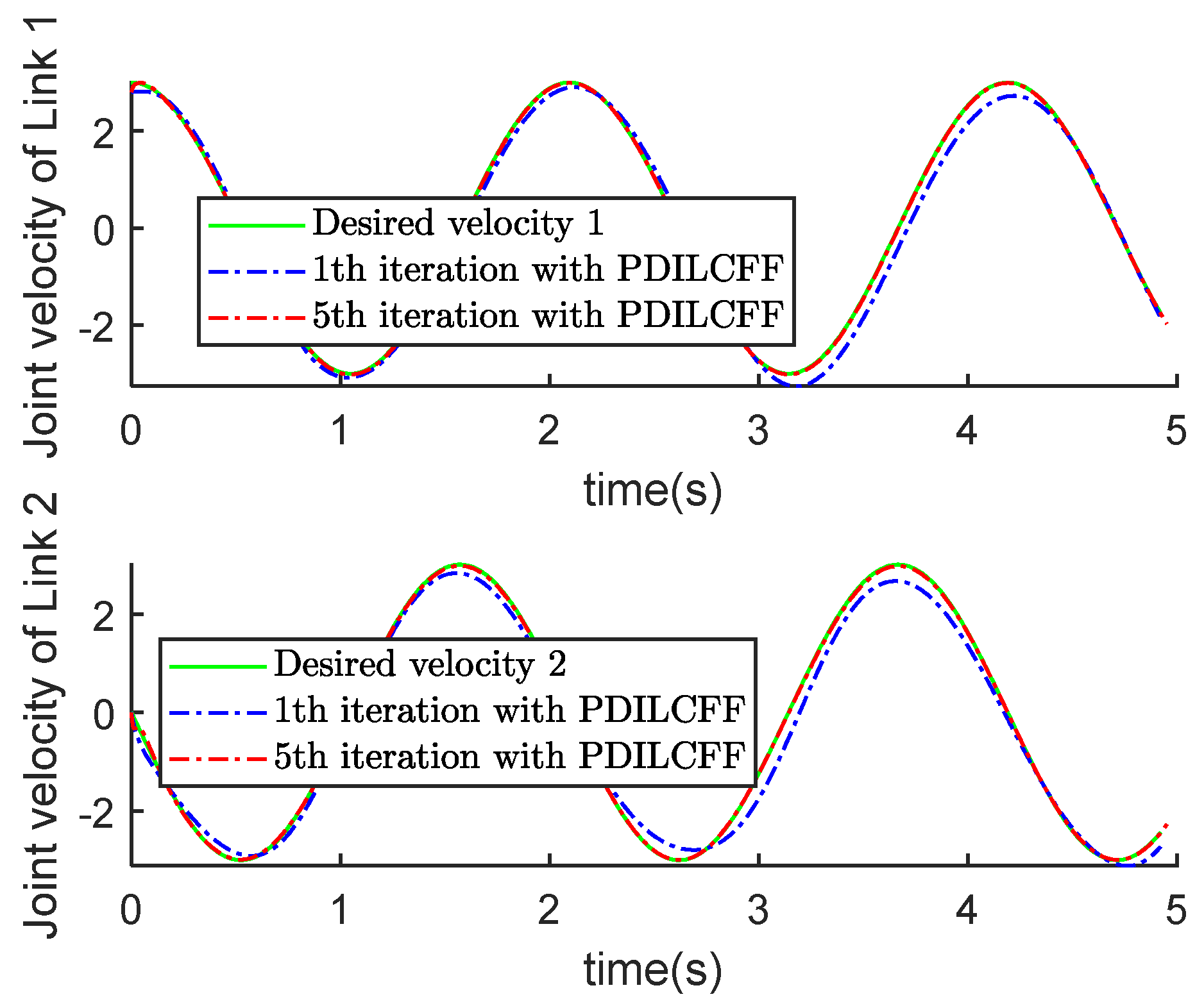
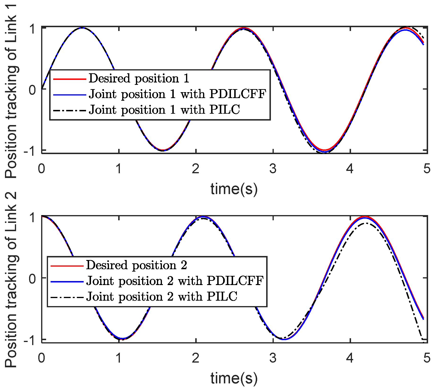
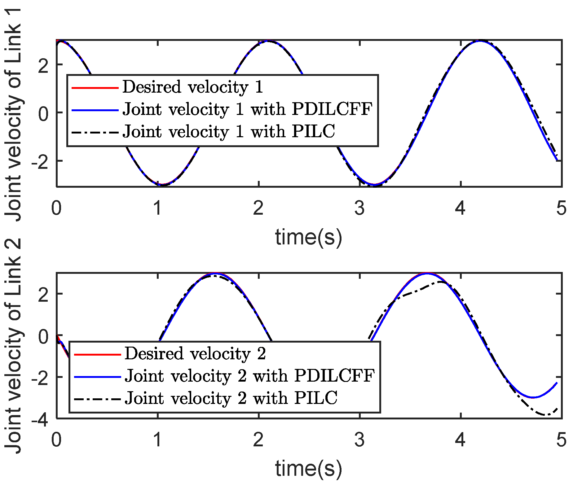
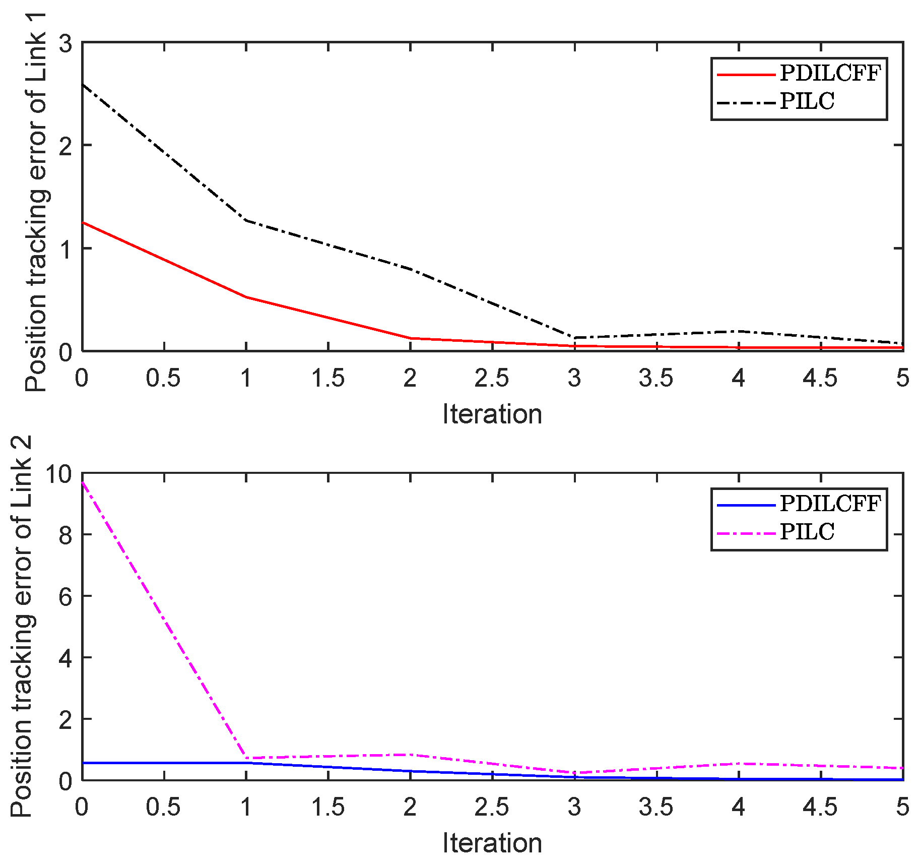
4. Simulation Study

Two simulation examples are provided to illustrate the effectiveness of the proposed PDILCFF scheme in this section. The PILC algorithm (25) is considered for comparison.

$${\mathit{u}}_{i+1}(t)={\mathit{u}}_i(t)+{\mathsf{\lambda }}_p{\mathit{e}}_i^{\ast }(t)$$

(25)

where ${\mathsf{\lambda }}_p$ is the gain matrix of the appropriate dimension.

Example 1.

Subway train tracking control

The parameters of the subway train dynamic model in [41], such as basic resistance coefficients and the mass and distribution constant for each vehicle, are given and omitted here for the sake of simplification. The disturbance is given by $\mathit{w}(t)=0.1Msin\left(t\right)e^{-3it}$. The initial values are $u_i(0)=0.01$, $x_i(0)=0.01$, and ${\dot{x}}_i(0)=0$. $T_{\min }=185\mathit{s}$, $T_{\min }=191\mathit{s}$.

The parameters of the proposed PDILCFF algorithm (9) and PILC algorithm (25) are $\beta =0.001$, $\mathit{H}=11$, $\mathit{K}=1.9\times {10}^5$, and ${\mathsf{\lambda }}_p=4600$. $\Vert (1-\beta )\mathit{I}-\mathit{HCB}\Vert =0<1$ satisfies the condition in Theorem 1.

Figure 2 shows the unit additional resistance profiles of the subway train system at the 2nd, 5th, 8th and 10th iterations. The additional resistance includes tunnel resistance, gradient resistance, and curve resistance.

Figure 3 and Figure 4 plot the speed tracking profiles with PDILCFF and PILC at the 2nd, 5th, 8th and 10th iterations in the time domain. Figure 5 and Figure 6 show the speed and position tracking profiles at the 10th iteration. Figure 7 and Figure 8 exhibit the maximum speed and position tracking error profiles in the iteration domain. Figure 9 and Figure 10 show the force contribution profiles for PDILCFF and PILC. From Figure 3, Figure 4, Figure 5, Figure 6, Figure 7 and Figure 8, we can see that the presented PDILCFF method has better convergence and control performance than the PILC method under the randomly varying iteration lengths for different iterations and disturbances.

Table 1 and Table 2 show a comparison of the maximum speed and position errors of the different algorithms in Example 1. It is clear that the proposed control algorithm has better tracking performance and convergence.

Table 1. Comparison of the maximum speed errors of different algorithms in Example 1.

Control Algorithm	The Maximum Speed Tracking Error of Different Iterations
	1	2	3	4	5	6	7	8	9	10
PDILCFF	22.23	7.58	2.78	1.43	0.60	0.73	0.51	0.38	0.50	0.42
PILC	58.58	32.04	57.46	35.00	28.49	29.70	29.71	23.73	38.02	51.19

Table 1. Comparison of the maximum speed errors of different algorithms in Example 1.

Control Algorithm	The Maximum Speed Tracking Error of Different Iterations
	1	2	3	4	5	6	7	8	9	10
PDILCFF	22.23	7.58	2.78	1.43	0.60	0.73	0.51	0.38	0.50	0.42
PILC	58.58	32.04	57.46	35.00	28.49	29.70	29.71	23.73	38.02	51.19

Table 2. Comparison of the maximum position errors of different algorithms in Example 1.

Control Algorithm	The Maximum Position Tracking Error of Different Iterations
	1	2	3	4	5	6	7	8	9	10
PDILCFF	1687	641	242	125	56	67	43	33	45	34
PILC	2014	641	2239	2538	1727	1188	883	676	514	796

Table 2. Comparison of the maximum position errors of different algorithms in Example 1.

Control Algorithm	The Maximum Position Tracking Error of Different Iterations
	1	2	3	4	5	6	7	8	9	10
PDILCFF	1687	641	242	125	56	67	43	33	45	34
PILC	2014	641	2239	2538	1727	1188	883	676	514	796

Example 2.

Two-degree-of-freedom robot manipulator [42].

$$\mathit{D}({\mathit{x}}_1){\dot{\mathit{x}}}_2+\mathit{C}({\mathit{x}}_1,{\mathit{x}}_2){\mathit{x}}_2+\mathit{G}({\mathit{x}}_1)+\mathit{w}(t)=\mathsf{\tau }$$

(26)

where ${\mathit{x}}_1=[x_{11},x_{12}]$ is the joint position vector. ${\mathit{x}}_2=[x_{21},x_{22}]$ is the velocity vector.$\mathsf{\tau }=[{\tau }_1,{\tau }_2]$ is the control input vector of two joint links. $\mathit{D}({\mathit{x}}_1)=\left[\begin{array}{cc}{d}_{11}& d_{12}\\ d_{21}& d_{22}\end{array}\right]$ is the inertia matrix.

$$\begin{gathered} d_{11}=m_1{l}_{c1}^2+m_2(l_1^2+l_{c2}^2+2l_1{l}_{c2}\cos (x_{12}))+I_1+I_2 \\ {d}_{12}=d_{21}=m_2(l_{c2}^2+l_1{l}_{c2}\cos (x_{12}))+I_2,d_{22}=m_2{l}_{c2}^2+I_2. \end{gathered}$$

$\mathit{C}({\mathit{x}}_1,{\mathit{x}}_2)=\left[\begin{array}{cc}{c}_{11}& c_{12}\\ c_{21}& c_{22}\end{array}\right]$ is the Coriolis–centripetal matrix.

$c_{11}=-m_2{l}_1{l}_{c2}{x}_{22}\sin (x_{12})$, $c_{21}=m_2{l}_1{l}_{c2}{x}_{21}\sin (x_{12})$

$c_{12}=-m_2{l}_1{l}_{c2}{x}_{22}\sin (x_{12})(x_{21}+x_{22})$, $c_{22}=0$.

$\mathit{G}({\mathit{x}}_1)={[G_1,G_2]}^T$ is gravity.

$G_1=(m_1{l}_{c2}+m_2{l}_1)g\cos (x_{11})+m_2{l}_{c2}g\cos (x_{11}+x_{12})$

$G_2=m_2{l}_{c2}g\cos (x_{11}+x_{12})$.

The parameters of the robot manipulator are $l_1=l_2=1 \mathrm{m}$, $l_{c1}=l_{c2}=0.5 \mathrm{m}$, $I_1=I_2=0.2 \mathrm{kg}\cdot {\mathrm{m}}^2$, and $g=9.81 {\mathrm{m}/\mathrm{s}}^2$. $m_1=0.9 \mathrm{kg}$ and $m_2=1 \mathrm{kg}$ represent the mass. The disturbance is $\mathit{w}(t)=[0.3\sin (t),0.1(1-e^{-t}]$. The desired trajectories are ${\mathit{x}}_{1d}={[\sin (3t),\cos (3t)]}^T$, and ${\mathit{x}}_{2d}={[3\cos (3t),-3\sin (3t)]}^T$.

The parameters of PDILCFF and PILC are given by $\beta =0.02$, $\mathit{K}=\left[\begin{array}{cc}0.3& 0\\ 0& 0.5\end{array}\right]$, $\mathit{H}=\left[\begin{array}{cc}200& 0\\ 0& 20\end{array}\right]$, ${\mathsf{\lambda }}_p=\left[\begin{array}{cc}0.8& 0\\ 0& 0.8\end{array}\right]$. $T_{\min }=4.9 \mathrm{s}$, and $T_{\min }=5.05 \mathrm{s}$. ${\mathit{x}}_1(0)=[0,2.8]$, ${\mathit{x}}_2(0)=[1.01,0]$, and $\mathsf{\tau }(0)=[0.1,0.1]$.

Figure 11 and Figure 12 plot the position and velocity tracking profiles of two links with PDILCFF at the 1st and 5th iterations in the time domain. Figure 13 and Figure 14 exhibit the position and velocity tracking profiles for PDILCFF and PILC at the 5th iteration. Figure 15 and Figure 16 give the maximum speed and position tracking error profiles in the iteration domain. Figure 11, Figure 12, Figure 13, Figure 14 and Figure 15 demonstrate that when the operation length of the robot manipulator system with disturbances varies randomly, the proposed PDILCFF method has better convergence and control performance than PILC.

Table 3. Comparison of the maximum velocity errors of different algorithms in Example 2.

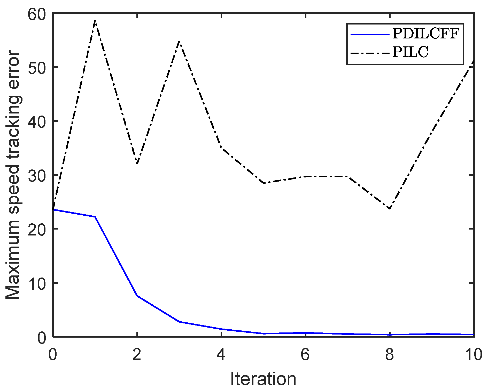
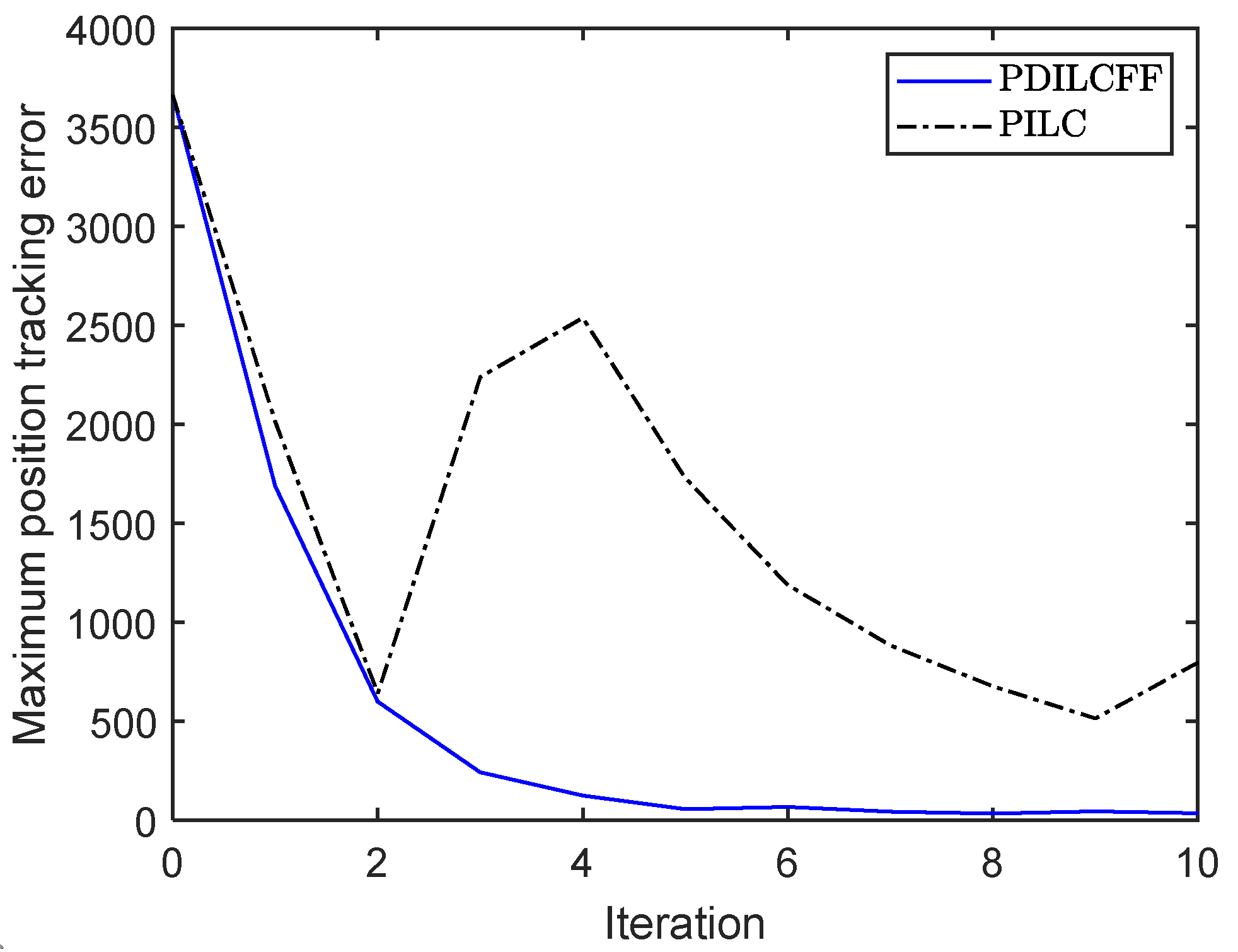
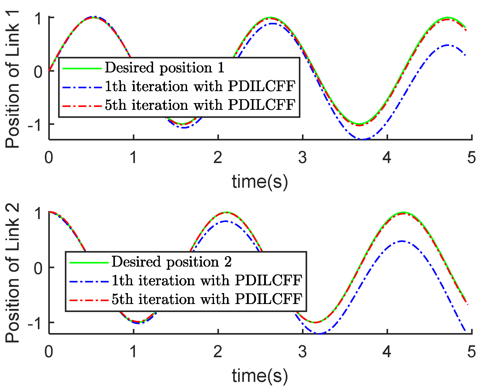
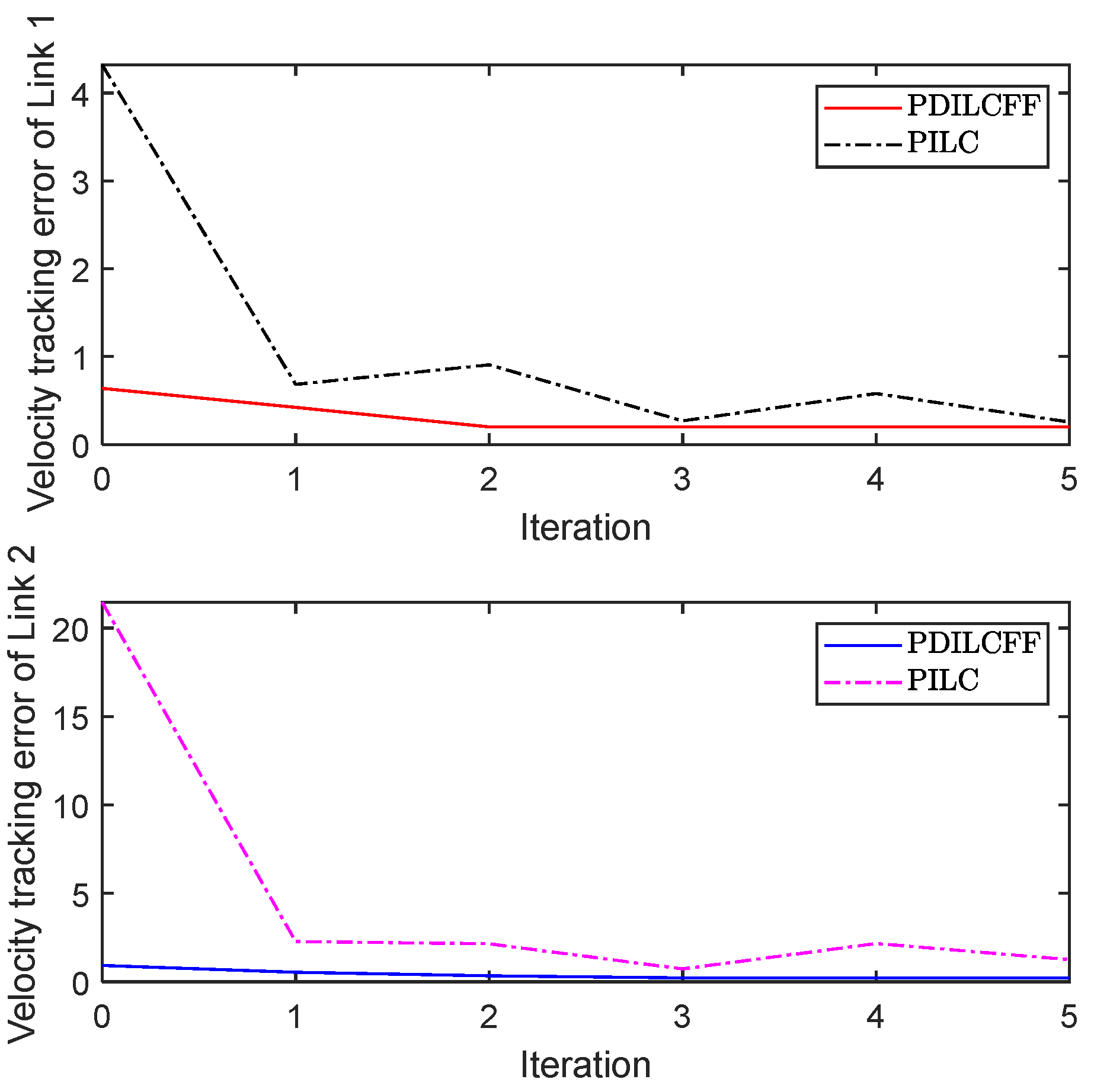
Control Algorithm	Link 1 of Different Iterations					Link 2 of Different Iterations
	1	2	3	4	5	1	2	3	4	5
PDILCFF	0.42	0.20	0.21	0.20	0.20	0.55	0.35	0.23	0.22	0.22
PILC	0.68	0.91	0.27	0.58	0.25	2.28	2.15	0.74	2.17	1.25

and

Table 4. Comparison of the maximum position errors of different algorithms in Example 2.

Control Algorithm	Link 1 of Different Iterations					Link 2 of Different Iterations
	1	2	3	4	5	1	2	3	4	5
PDILCFF	0.53	0.13	0.25	0.04	0.03	0.58	0.30	0.10	0.04	0.03
PILC	1.28	0.80	0.13	0.19	0.08	0.73	0.84	0.24	0.55	0.40

show a comparison of the maximum speed and position errors of the different algorithms in Example 2. It can be seen that the proposed control algorithm has better tracking performance and convergence.

The simulation results of Section 4 demonstrate that the proposed PDILCFF has good control effect and robustness and verifies the correctness of Theorem 1.

Remark 2.

Considering iteration-varying trial lengths, the proposed PDILCFF algorithm is closely related to symmetry.

(1) The PDILCFF method takes advantage of time symmetry. The essence of iterative learning control is to learn and optimize the process of repeating the same task, and each iteration can be regarded as a time period. If the system meets certain conditions, different iteration cycles have similarities or symmetries in the time dimension. Time symmetry enhances the effectiveness of iterative learning control, enabling it to make better use of historical information. For example, for the control task of a robotic arm with periodic motion, each complete motion cycle can be regarded as a repetition of the previous cycle, but the control input is constantly optimized during the iterative process. This time symmetry enables iterative learning control to effectively learn from historical iterative data and symmetrically apply the error information of the previous period to the control and adjust subsequent periods, gradually reducing the error and improving system performance.

(2) The PDILCFF method utilizes dynamic symmetry. There is a certain symmetrical relationship between the treatment methods of errors and their rates of change in the proportional link and the differential link. The proportional link is adjusted according to the current error magnitude, while the differential link is adjusted according to the error change rate. The two cooperate with each other to control system dynamics from a symmetrical perspective. Dynamic symmetry enhances the controller’s response to the dynamic changes of the system.

(3) The PDILCFF method utilizes spatial symmetry. For example, during the movement of the robotic arm, the movements of each joint axis cooperate with each other to jointly complete complex spatial tasks, and the movement relationship among them contains spatial symmetry. Meanwhile, iterative learning control can utilize spatial symmetry to share and transfer control experience and error information of different axes at the same task stage, optimizing the overall control performance. Spatial symmetry ensures the stability and accuracy of the overall motion of the system in systems involving spatial motion.

The comprehensive application of these symmetries enables the PDILCFF method to work more efficiently in complex control systems, enhancing the robustness and reliability of the system.

5. Conclusions

This paper has proposed a PDILCFF method for nonlinear systems with randomly varying iteration lengths and state and measurement disturbances. Firstly, considering the randomly varying iteration lengths, a modified tracking error was designed. Secondly, a PDILCFF scheme was proposed to deal with the problems of initial state shift, state disturbances and measurement disturbances. The compression mapping method was exploited to obtain a convergence property of the proposed PDILCFF scheme, which guaranteed that the tracking error was bounded convergence, and when the disturbances disappeared, the tracking error converged to zero. Finally, two simulation examples were provided to verify the effectiveness of the theoretical studies. In future work, by drawing on the control algorithm and analysis method proposed in this paper, we will study multi-agent consensus and formation problems under randomly varying iteration lengths, initial state shifts and disturbances.

References

- Arimoto, S.; Kawamura, S.; Miyazaki, F. Bettering operation of robots by learning. J. Field Robot. 1984, 1, 123–140. [Google Scholar] [CrossRef]
- Xu, J.-X. A survey on iterative learning control for nonlinear systems. Int. J. Control. 2011, 84, 1275–1294. [Google Scholar] [CrossRef]
- Tan, W.; Hou, Z.; Li, Y.X. Robust data-driven iterative learning control for high-speed train with aperiodic DoS attacks and communication delays. IEEE Trans. Intell. Vehicl. 2024, 1–10. [Google Scholar] [CrossRef]
- Li, S.; Li, X. Finite-time extended state observer-based iterative learning control for nonrepeatable nonlinear systems. Nonlinear Dyn. 2025, 113, 16531–16543. [Google Scholar] [CrossRef]
- Arimoto, S. Learning control theory for robotic motion. Int. J. Adapt. Control. Signal Process. 1990, 4, 543–564. [Google Scholar] [CrossRef]
- Saab, S.S. On the P-type learning control. IEEE Trans. Automat. Contr. 1994, 39, 2298–2302. [Google Scholar] [CrossRef]
- Xu, J.X.; Jin, X. State-Constrained Iterative Learning Control for a Class of MIMO Systems. IEEE Trans. Automat. Contr. 2013, 58, 1322–1327. [Google Scholar] [CrossRef]
- Bai, L.; Feng, Y.-W.; Li, N.; Xue, X.-F.; Cao, Y. Data-Driven Adaptive Iterative Learning Method for Active Vibration Control Based on Imprecise Probability. Symmetry 2019, 11, 746. [Google Scholar] [CrossRef]
- Hou, Z.S.; Chi, R.; Gao, H. An overview of dynamic-linearization-based data-driven control and applications. IEEE Trans. Ind. Electron. 2017, 64, 4076–4090. [Google Scholar] [CrossRef]
- Yu, X.; Chen, T. Distributed Iterative Learning Control of Nonlinear Multiagent Systems Using Controller-Based Dynamic Linearization Method. IEEE Trans. Cybern. 2023, 54, 4489–4501. [Google Scholar] [CrossRef]
- Zhang, H.; Chi, R.; Huang, B.; Hou, Z. Compensatory Data-Driven Networked Iterative Learning Control with Communication Constraints and DoS Attacks. IEEE Trans. Autom. Sci. Eng. 2025, 22, 10728–10740. [Google Scholar] [CrossRef]
- Chi, R.; Hou, Z.S.; Huang, B.; Jin, S. A unified data-driven design framework of optimality-based generalized iterative learning control. Comput. Chem. Eng. 2015, 77, 10–23. [Google Scholar] [CrossRef]
- Chi, R.; Liu, X.; Zhang, R.; Hou, Z.S.; Huang, B. Constrained data-driven optimal iterative learning control. J. Process Contr. 2017, 55, 10–29. [Google Scholar] [CrossRef]
- Huang, Y.; Tao, H.; Chen, Y.; Rogers, E.; Paszke, W. Point-to-point iterative learning control with quantised input signal and actuator faults. Int. J. Control. 2024, 97, 17. [Google Scholar] [CrossRef]
- Wang, L.; Dong, L.; Chen, Y.; Wang, K.; Gao, F. Iterative Learning Control for Actuator Fault Uncertain Systems. Symmetry 2022, 14, 1969. [Google Scholar] [CrossRef]
- Tayebi, A. Adaptive iterative learning control for robot manipulators. Automatica 2004, 40, 1195–1203. [Google Scholar] [CrossRef]
- Yin, C.; Xu, J.-X.; Hou, Z. A high-order internal model based iterative learning control scheme for nonlinear systems with time-iteration-varying parameters. IEEE Trans. Automat. Contr. 2010, 55, 2665–2670. [Google Scholar] [CrossRef]
- Chi, R.H.; Hou, Z.S.; Huang, B. Optimal iterative learning control of batch processes: From model-based to data-driven. Zidonghua Xuebao/Acta Autom. Sin. 2017, 43, 917–932. [Google Scholar]
- Liu, G.; Hou, Z.S. Cooperative adaptive iterative learning fault-tolerant control scheme for multiple subway trains. IEEE Trans. Cybern. 2022, 52, 1098–1111. [Google Scholar] [CrossRef]
- Liu, G.; Hou, Z.S. RBFNN-based adaptive iterative learning fault-tolerant control for subway trains with actuator faults and speed constraint. IEEE Trans. Syst. Man Cybern. Syst. 2021, 51, 5785–5799. [Google Scholar] [CrossRef]
- Hou, Z.S.; Yan, J.; Xu, J.-X.; Li, Z. Modified iterative-learning-control-based ramp metering strategies for freeway traffic control with iteration-dependent factors. IEEE Trans. Intell. Transp. Syst. 2012, 13, 606–618. [Google Scholar] [CrossRef]
- Hou, Z.; Xu, X.; Yan, J.; Xu, J.X.; Xiong, G. A complementary modularized ramp metering approach based on iterative learning control and ALINEA. IEEE Trans. Intell. Transp. Syst. 2011, 12, 1305–1318. [Google Scholar] [CrossRef]
- Longman, R.W.; Mombaur, K.D. Investigating the use of iterative learning control and repetitive control to implement periodic gaits. Lect. Notes Control Inform. Sci. 2006, 340, 189–218. [Google Scholar]
- Yu, Q.; Hou, Z.S. Adaptive fuzzy iterative learning control for high-speed trains with both randomly varying operation lengths and system constraints. IEEE Trans. Fuzzy Syst. 2021, 29, 2408–2418. [Google Scholar] [CrossRef]
- Seel, T.; Schauer, T.; Raisch, J. Iterative learning control for variable pass length systems. In Proceedings of the the 18th IFAC World Congress, Milano, Italy, 28 August–2 September 2011; pp. 4880–4885. [Google Scholar]
- Guth, M.; Seel, T.; Raisch, J. Iterative learning control with variable pass length applied to trajectory tracking on a crane with output constraints. In Proceedings of the 52nd IEEE Conference on Decision and Control, Florence, Italy, 10–13 December 2013; pp. 6676–6681. [Google Scholar]
- Li, X.; Xu, J.-X.; Huang, D. An iterative learning control approach for linear time-invariant systems with randomly varying trial lengths. IEEE Trans. Automat. Contr. 2014, 59, 1954–1960. [Google Scholar] [CrossRef]
- Li, X.; Xu, J.-X.; Huang, D. Iterative learning control for nonlinear dynamic systems with randomly varying trial lengths. Int. J. Adapt. Control Signal Process 2015, 29, 1341–1353. [Google Scholar] [CrossRef]
- Shen, D.; Zhang, W.; Wang, Y.; Chien, C.J. On almost sure and mean square convergence of P-type ILC under randomly varying iteration lengths. Automatica 2016, 63, 359–365. [Google Scholar] [CrossRef]
- Li, X.; Shen, D. Two novel iterative learning control schemes for systems with randomly varying trial lengths. Syst. Control. Lett. 2017, 107, 9–16. [Google Scholar] [CrossRef]
- Wang, L.; Li, X.; Shen, D. Sampled-data iterative learning control for continuous-time nonlinear systems with iteration-varying lengths. Int. J. Robust Nonlinear Control. 2018, 28, 3073–3091. [Google Scholar] [CrossRef]
- Shen, D.; Xu, J.-X. Robust learning control for nonlinear systems with nonparametric uncertainties and nonuniform trial lengths. Int. J. Robust Nonlinear Control. 2019, 29, 1302–1324. [Google Scholar] [CrossRef]
- Shen, D.; Xu, J.-X. Adaptive learning control for nonlinear systems with randomly varying iteration lengths. IEEE Trans. Neural. Networ. 2019, 30, 1119–1132. [Google Scholar] [CrossRef] [PubMed]
- Liu, G.; Hou, Z. Adaptive iterative learning fault-tolerant control for state constrained nonlinear systems with randomly varying iteration lengths. IEEE Trans. Neural. Networ. 2024, 35, 1735–1749. [Google Scholar] [CrossRef]
- Bu, X.; Wang, S.; Hou, Z.S.; Liu, W. Model free adaptive iterative learning control for a class of nonlinear systems with randomly varying iteration lengths. J. Frankl. Inst. 2019, 356, 2491–2504. [Google Scholar] [CrossRef]
- Xu, R.; Chen, H.; Tang, Y.; Long, X. Model-free predictive iterative learning safety-critical consensus control for multi-agent systems with randomly varying trial lengths. Syst. Control. Lett. 2025, 196, 105987. [Google Scholar] [CrossRef]
- Shen, D.; Zhang, W.; Xu, J.-X. Iterative learning control for discrete nonlinear systems with randomly iteration varying lengths. Syst. Control. Lett. 2016, 96, 81–87. [Google Scholar] [CrossRef]
- Wei, Y.; Li, X. Robust higher-order ILC for non-linear discrete-time systems with varying trail lengths and random initial state shifts. IET Control. Theory Appl. 2017, 11, 2440–2447. [Google Scholar] [CrossRef]
- Liu, Y.; Fan, Y.; Ao, Y.; Jia, Y. An iterative learning approach to formation control of discrete-time multi-agent systems with varying trial lengths. Int. J. Robust Nonlinear Control. 2022, 32, 9332–9346. [Google Scholar] [CrossRef]
- Hussain, M.; Muslim, F.B.; Khan, O.; Saqib, N.u. Robust anti-windup control atrategy for uncertain nonlinear system with time delays. Arab. J. Sci. Eng. 2022, 47, 3847–3860. [Google Scholar] [CrossRef]
- Liu, G.; Hou, Z. Adaptive iterative learning control for subway trains using multiple-point-mass dynamic model under speed constraint. IEEE Trans. Intell. Transp. Syst. 2021, 22, 1388–1400. [Google Scholar] [CrossRef]
- Jin, X. Iterative learning control for MIMO nonlinear systems with iteration-varying trial lengths using modified composite energy function analysis. IEEE Trans. Cybern. 2021, 51, 6080–6090. [Google Scholar] [CrossRef]