Dual Graph Laplacian RPCA Method for Face Recognition Based on Anchor Points

Abstract

High-dimensional data often contain noise and undancy, which can significantly undermine the performance of machine learning. To address this challenge, we propose an advanced robust principal component analysis (RPCA) model that integrates bidirectional graph Laplacian constraints along with the anchor point technique. This approach constructs two graphs from both the sample and feature perspectives for a more comprehensive capture of the underlying data structure. Moreover, the anchor point technique serves to substantially reduce computational complexity, making the model more efficient and scalable. Comprehensive evaluations on both GTdatabase and VGG Face2 dataset confirm that anchor-based methods maintain competitive accuracy with standard graph Laplacian approaches (within 0.5–2.0% difference) while achieving significant computational speedups of 5.7–27.1% and 12.9–14.6% respectively. The consistent performance across datasets, from controlled laboratory conditions to challenging real-world scenarios, demonstrates the robustness and scalability of the proposed anchor technique.

1. Introduction

With the rapid advancement of artificial intelligence technology, machine learning has found extensive applications in various domains, including information retrieval, person re-identification, and face recognition. In execution of these tasks, data are frequently represented as high-dimensional, inevitably exhibiting correlations and containing substantial redundancy and noisy features. The redundant and noisy features may undermine the performance of subsequent tasks, such as clustering, classification, retrieval, or reconstruction. Hence, high-dimensional data pose the “curse of dimensionality” challenge to machine learning algorithms. To enhance the efficacy of machine learning methods, it is imperative to employ feature selection techniques to eliminate irrelevant, redundant, and noisy features from high-dimensional data.

Face recognition has been a prominent area of focus in machine learning. Principal component analysis (PCA) and its various variants have been successfully used for face recognition [1,2,3,4,5,6,7]. Sirovich and Kirby firstly applied PCA to efficiently represent the face images in a lower-dimensional space. Based on the Karhunen-Loeve procedure for the characterization of human faces [1], Turk and Pentland presented the eigenface method for face recognition [2]. Subsequently, Yang et al. [3] proposed a novel technique known as 2DPCA to enhance the recognition rate of conventional PCA. Early PCA methods primarily addressed grayscale images by representing each image as a vector. Specifically, consider a data matrix $X=(x_1,\dots ,x_n)\in {\mathbb{R}}^{m\times n}(m\gg n)$ with rows representing features and columns representing samples. PCA is typically utilized to identify the optimal principal directions $U=(u_1,\dots ,u_k)\in {\mathbb{R}}^{m\times k}(U^{T}U=I)$ that define the low-dimensional (k-dim) subspace. The projected data points with the low subspace U can be denoted as the matrix $V^T=(v_1,\dots ,v_n)\in {\mathbb{R}}^{k\times n}$. Then the traditional PCA finds U and V with the following constrained problem

$$\underset{U,V}{\mathrm{a}\mathrm{r}\mathrm{g} \mathrm{m}\mathrm{i}\mathrm{n}}{ \Vert \mathrm{X}-{\mathrm{UV}}^T \Vert }_F^2,s.t.V^{T}V=I.$$

(1)

However, the performance of traditional PCA is typically poor. Outliers, which are prevalent in many scenarios due to factors such as sudden intense interference during transmission, sensor failures, and calibration errors, can significantly impact the results. To address this problem, robust PCA (RPCA) [8] has been proposed to decompose the observed matrix data into a sum of low-rank and sparse matrices, ensuring that no abnormal data disrupts the system. Intuitively, the RPCA can be formulated as the following minimization problem

$$\underset{L,S}{\mathrm{a}\mathrm{r}\mathrm{g} \mathrm{m}\mathrm{i}\mathrm{n}} \mathrm{r}\mathrm{a}\mathrm{n}\mathrm{k}\left(L\right)+\lambda {\parallel S\parallel }_0,s.t.X=L+S.$$

(2)

To address (2) more effectively, researchers relaxed the rank function by the nuclear norm [9,10], thereby transforming the problem into a convex optimization problem, as follows

$$\underset{L,S}{\mathrm{a}\mathrm{r}\mathrm{g} \mathrm{m}\mathrm{i}\mathrm{n}}{\parallel L\parallel }_{*}+\lambda {\parallel S\parallel }_1,s.t.X=L+S.$$

(3)

Although the convex model can accurately yield low-rank and sparse matrices under relatively mild conditions, it overlooks the presence of the noise with small magnitudes. This oversight is significant because, in real-world scenarios, data often suffer from contamination by the noise. To address this limitation, Zhou et al. [11] introduced a method that decomposed the data matrix into three components: a low-rank matrix, a sparse matrix, and a noise matrix

$$\underset{U,V,S}{\mathrm{a}\mathrm{r}\mathrm{g} \mathrm{m}\mathrm{i}\mathrm{n}}{\parallel X-UV-S\parallel }_F^2+\lambda {\parallel S\parallel }_1,s.t.X=L+S+G,L=UV.$$

(4)

However, color information is not fully exploited, despite being a crucial characteristic for enhancing image discriminability. To address this, Torres et al. [4] extended traditional PCA to color face recognition by applying it separately to the color channels, with the final result obtained by fusing the outcomes from all three channels. Building upon this foundation, Yang et al. [5] proposed a general discriminant model for color face recognition, which employs a set of color component combination coefficients to merge the three color channels into a single channel, representing color face images. Furthermore, Xiang et al. [6] introduced a matrix-representation model for color images based on the PCA framework and applied 2DPCA to compute optimal projection vectors for feature extraction. A more generalized approach, as opposed to the aforementioned channel-wise processing techniques, involves representing color images through quaternion matrices, which inherently encode color channels in a holistic manner. This avoids artificial separation of Red-Green-Blue (RGB) components and preserves inter-channel correlations. Recent works have utilized quaternion PCA (QPCA) for dimensionality reduction [12,13,14,15,16,17,18]. Notably, Wang et al. [19] demonstrated that the matrix equation AXB = C is fundamental to optimizing quaternion-based models, where solutions over quaternions and their extensions enable efficient color image processing while preserving color integrity, particularly in feature extraction and multi-channel image encryption. In complementary technical advancement, Jia et al. [20] constructed general solutions for split-quaternion tensor equations, extending the processing scope to dynamic videos while significantly enhancing computational efficiency and security through the pseudo-Euclidean properties of split quaternions.

The purpose of these non-linear dimensionality reduction techniques is to find a representation of points in a low-dimensional space, in which all points still maintain the similarity in the lower-dimensional space. In recent years, optimization models that combine linear and non-linear dimensionality reduction methods, especially graph Laplacian embedding, have demonstrated their effectiveness. Cai et al. [21] proposed a graph regularized non-negative matrix factorization (GNMF) method, which combined graph structure and non-negative matrix factorization for an improved compact representation of the original data. Building upon this, Jiang et al. [22] developed graph Laplacian PCA (GLPCA), which sought a low-dimensional representation of image data with significant improvement in clustering and image reconstruction by incorporating graph structures and PCA. Further advancing this line of research, Feng et al. [23] employed PGLPCA based on graph Laplacian regularization and Lp-norm for feature selection and tumor clustering. Parallel developments include Liu et al.’s [24] graph Laplacian matrix formulation for semi-supervised feature extraction and Wang et al.’s [25] Laplacian regularized low-rank representation (LLRR), which successfully captures the intrinsic geometric structure of gene expression data for improved tumor sample clustering. Building on these methods, Yang et al. [26] developed an innovative online algorithm using Monte Carlo sampling for sparse graph-constrained matrix optimization, effectively solving feature selection problems while maintaining manifold structures.

To fully exploit the spatial and spectral features of images, we propose constructing two complementary graphs. One graph captures temporal or sample-based relationships among superpixels e.g., the columns of the data matrix X, while the other encodes spatial relationships among pixel locations e.g., the rows of the data matrix X. By integrating these two graphs, we effectively harness both spatial and spectral information, resulting in a more comprehensive representation of the image data. This dual-graph strategy enhances the model’s capacity to capture the inherent structure of the data, thereby improving performance in tasks like image segmentation, classification, and reconstruction.

Furthermore, to expedite the construction of the graph Laplacian matrix and streamline the computational process, we introduce the notion of anchor points. These anchor points serve as representative samples that encapsulate the data’s structure, significantly reducing the number of pairwise comparisons needed during graph construction. Instead of calculating relationships between all data points, we select a subset of anchor points (using methods such as random sampling, K-means, or other clustering techniques) and build the graph based on the relationships between data points and these anchors. This approach not only reduces computational complexity but also preserves the geometric and relational properties of the data, enabling the method to scale to large datasets without compromising the quality of the embeddings or the performance of downstream tasks.

The main contributions of our work are outlined as follows

1.

Integration of Graph Laplacian Embedding with RPCA We incorporate graph Laplacian embedding into RPCA to account for the spatial information inherent in the data. By representing the data as a graph, where nodes correspond to data points and edges reflect pairwise relationships (such as similarity or distance), the graph Laplacian matrix effectively captures the dataset’s underlying geometric structure.

2.

Exploitation of Two-Sided Data Structure We leverage a dual perspective by obtaining the graph Laplacian from both the sample and feature dimensions. This approach enables us to capture intrinsic relationships not only among data points (samples) but also among features, thereby providing a more holistic representation of the data.

3.

Introduction of Anchors for Computational Efficiency We introduce the concept of anchors to enhance the model’s running speed and reduce computational complexity. Anchors serve as representative points that summarize the data’s structure, thereby minimizing the number of pairwise comparisons needed during graph construction. Instead of computing relationships between all data points, we select a subset of anchors (using methods like random sampling, K-means, or other clustering techniques) and construct the graph based on the relationships between data points and these anchors. This method significantly reduces the size of the adjacency matrix and, consequently, the computational burden associated with the graph Laplacian.

The rest of the paper is organized as follows. Section 2 provides an overview of the fundamental theoretical foundations including quaternion and quaternion matrix, graphs, graph Laplacian embedding and anchor point technique. In Section 3, we present the proposed algorithm and methodology. Subsequently, Section 4 demonstrates the experimental results using real-world facial image datasets. Finally, Section 5 concludes the paper with a summary of our findings and contributions.

2. Preliminaries

2.1. Quaternion and Quaternion Matrix

Introduced by mathematician Hamilton in 1843 [27], quaternion generalizes complex numbers by incorporating one real part and three imaginary parts. A quaternion can be expressed as

$$a=a_0+a_1\mathbf{i}+a_2\mathbf{j}+a_3\mathbf{k},$$

(5)

where $a_0,a_1,a_2,a_3\in \mathbb{R}$, and $\mathbf{i},\mathbf{j},\mathbf{k}$ are three imaginary units that follow the multiplication rules

$${\mathbf{i}}^2={\mathbf{j}}^2={\mathbf{k}}^2=-1,\mathbf{i}\mathbf{j}=-\mathbf{j}\mathbf{i}=\mathbf{k},\mathbf{j}\mathbf{k}=-\mathbf{k}\mathbf{j}=\mathbf{i},\mathbf{k}\mathbf{i}=-\mathbf{i}\mathbf{k}=\mathbf{j}.$$

(6)

The conjugate and modulus of quaternion a are defined as follows

$$\overline{\mathrm{a}}={\mathrm{a}}_0-{\mathrm{a}}_1\mathbf{i}-{\mathrm{a}}_2\mathbf{j}-{\mathrm{a}}_3\mathbf{k},$$

(7)

$$\left|a\right|=\sqrt{{\left(a_0\right)}^2+{\left(a_1\right)}^2+{\left(a_2\right)}^2+{\left(a_3\right)}^2}.$$

(8)

A quaternion matrix $A\in {\mathbb{Q}}^{m\times n}$ takes the form

$$A=A_0+A_1\mathbf{i}+A_2\mathbf{j}+A_3\mathbf{k},$$

(9)

with $A_0,\dots ,A_3\in {\mathbb{R}}^{m\times n}$, and its conjugate transposed matrix is given by $A^{*}=A_0^T-A_1^T\mathbf{i}-A_2^T\mathbf{j}-A_3^T\mathbf{k}$. A pure quaternion matrix provides a representation for color images, with its three imaginary components $A_1,A_2,A_3$ corresponding to the red, green, and blue channels, respectively. Furthermore, the real representation method is a widely used technique for transforming quaternion matrices into the corresponding real matrices, the real representation of the matrix A is shown as

$${\gamma }_A=\left(\begin{array}{cccc}{A}_0& -A_2& -A_1& -A_3\\ A_2& A_0& -A_3& A_1\\ A_1& A_3& A_0& -A_2\\ A_3& -A_1& A_2& A_0\end{array}\right),$$

(10)

and the first block column of ${\gamma }_A$ is denoted by

$${\gamma }_{A,c}=\left[\begin{array}{c}{A}_0\\ A_2\\ A_1\\ A_3\end{array}\right].$$

(11)

Property 1.

For $A,B\in {\mathbb{Q}}^{m\times n},C\in {\mathbb{Q}}^{n\times s}$, the following properties hold [28].

1.

${\gamma }_{A+B}={\gamma }_A+{\gamma }_B,{\gamma }_{AC}={\gamma }_A{\gamma }_C$.

2.

${\gamma }_{A^{*}}={\gamma }_A^T$, where ${(·)}^T$ denotes transpose operation.

3.

A is a column unitary matrix if and only if ${\gamma }_A$ is a column orthogonal matrix.

2.2. Graph

Let $G=(V,E)$ be an undirected weighted graph. The weight value between $v_i$ and $v_j$ is denoted by $w_{ij}$. If there is no edge between $v_i$ and $v_j$, i.e., $(v_i,v_j)\notin E$, then $w_{ij}=0$. The matrix $W=\left(w_{ij}\right)(i,j=1,\dots ,n)$ is called the adjacency matrix of G. We define the degree matrix D, which is a diagonal matrix whose diagonal entry $D_{ii}$ equals to the sum of weights of all edges incident to i, i.e., $d_i={\sum }_{j=1}^n{w}_{ij}$. Subsequently, the graph Laplacian matrix is defined as follows

$$L=D-W.$$

(12)

In some applications, the normalized graph Laplacian is used, defined as

$$L_{norm}=I-D^{-{\displaystyle \frac{1}{2}}}{WD}^{-{\displaystyle \frac{1}{2}}}.$$

(13)

Property 2.

Let L denote a graph Laplacian matrix. Then the following properties hold [29].

1.

For each vector ${(f_1,\dots ,f_n)}^{\prime }=f\in {\mathbb{R}}^n$, we have

$$f^{\prime }Lf={\displaystyle \frac{1}{2}}\sum _{i=1}^n{w}_{ij}{\left(f_i-f_j\right)}^2.$$

(14)

2.

L is symmetric and positive semi-definite.

3.

The smallest eigenvalue of L is 0, and corresponding eigenvector is 1 whose elements are all ones.

4.

L has n non-negative real eigenvalues $0={\lambda }_1\le {\lambda }_2\le \dots \le {\lambda }_n$.

2.3. Graph Laplacian Embedding

Graph Laplacian embedding has emerged as a widely-used technique in nonlinear manifold learning, aiming to preserve the local geometric structure of data. The underlying assumption is that points which are close in the original data space should maintain their proximity in the embedded space. To achieve this, a nearest neighbor graph is constructed to capture and model the local relationships among data points.

Given the data matrix $X=(x_1,\dots ,x_n)\in {\mathbb{R}}^{m\times n}$, where $x_i$$(i=1,\dots ,n)$ denotes a data sample or one vertex in the graph. For each data point $x_i$, we connect each $x_i$ to its k nearest neighbors. Here, we adopt Euclidean distance $w_{ij}=\sqrt{{\sum }_{d=1}^m{(x_{i,d}-x_{j,d})}^2}$ to measure the similarity between the data samples.

Let $Z=(z_1,\dots ,z_n)\in {\mathbb{R}}^{k\times n}$ represent embedding coordinates of data samples $X=(x_1,\dots ,x_n)\in {\mathbb{R}}^{m\times n}$. The dissimilarity of the two data points in the lower-dimensional space can be measured by the Euclidean distance. Define the dissimilarity of the two data points in the lower-dimensional space as $d(z_i,z_j)=\left|\right|z_i-z_j{\left|\right|}^2$, combining with the weight matrix W, the smoothness of the low-dimensional representation can be measured by minimizing the following equation [30]

$$\begin{array}{cc}\hfill \mathrm{S}& ={\displaystyle \frac{1}{2}}\sum _{i,j=1}^n{\parallel z_i-z_j\parallel }^2{w}_{ij}\hfill \\ & =\sum _{i=1}^n{z}_i^T{z}_i{D}_{ii}-\sum _{i,j=1}^n{z}_i^T{z}_j{w}_{ij}\hfill \\ & =Tr\left(V^{T}DV\right)-Tr\left(V^{T}WV\right)=Tr\left(V^{T}LV\right),\hfill \end{array}$$

(15)

where $D=diag(d_1,\dots ,d_n)$ is a diagonal matrix, and $L=D-W$ is the graph Laplacian matrix.

2.4. Anchors

Anchor point techniques play a critical role in data representation and learning, effectively reducing computational costs while capturing the underlying structure of the data. In practice, anchors serve as critical and highly representative entities within data samples, functioning similarly to a basis set in linear space. Given a dataset $X=(x_1,x_2,\dots ,x_n)\in {\mathbb{R}}^{m\times n}$, anchor points $A=(a_1,a_2,\dots ,a_k)\in {\mathbb{R}}^{m\times k}$ with $k\ll n$, act as reference points in the data space. These can be strategically selected based on prior knowledge, such as class centers, or learned through methods like K-means clustering. The primary advantage of using anchors, as discussed in this paper, is their ability to rapidly and efficiently construct similarity matrices. This characteristic endows anchors with significant benefits for handling large-scale datasets and uncovering latent relationships among data samples. Additionally, in the following context, various methodologies for anchor generation will be discussed.

1.

K-means method for anchor points

We adopt the K-means clustering algorithm to derive a set of anchor points, which serve as representative prototypes for the underlying data distribution. Considering a dataset $X=(x_1,x_2,\dots ,x_n)\in {\mathbb{R}}^{m\times n}$, the K-means algorithm aims to partition X into k disjoint clusters $C=\{C_1,C_2,\dots ,C_k\}$ by minimizing the within-cluster sum of squares, formulated as [31]

$$f\left(x\right)=\sum _{i=1}^k\sum _{x\in C_i}{\parallel x-u_i\parallel }^2,$$

(16)

where $C_i$ denotes the i-th cluster and $u_i$ is its centroid, namely the anchor points.

2.

BKHK method for anchor points

The Balanced and Hierarchical K-means (BKHK) algorithm is a hierarchical anchor point selection method that combines K-means and hierarchical clustering to recursively construct evenly distributed anchor points, thereby improving representation ability. In contrast to conventional K-means algorithms that execute a single-step partitioning of the dataset into a predetermined number of clusters, BKHK employs a hierarchical partitioning strategy. It recursively divides the dataset X into m sub-clusters, performing binary K-means at each step. This process continues until the desired number of clusters is achieved. The objective function of Balanced Binary K-means is defined as follows [32]

$$\underset{H\in {\mathbb{B}}^{n\times 2},1_n^{T}H=[\lfloor {\displaystyle \frac{n}{2}}\rfloor ,n-\lfloor {\displaystyle \frac{n}{2}}\rfloor ]}{\mathrm{a}\mathrm{r}\mathrm{g} \mathrm{m}\mathrm{i}\mathrm{n}}{\parallel X-C{H}^T\parallel }_F^2,$$

(17)

where $C\in {\mathbb{R}}^{d\times 2}$ represents the two class centers, and $H\in {\mathbb{B}}^{n\times 2}$ is the class indicator matrix.

The construction of the similarity matrix based on representative anchors is a well-explored problem. In our approach, we choose to measure the distance using the Euclidean distance. To be specific, our objective is to learn a similarity matrix $Z\in {\mathbb{R}}^{n\times m}$, in a way that a smaller distance corresponds to a larger affinity value. This allows us to formulate the optimization problem as follows

$$\underset{z^i{1}_m=1,z^i>0}{\mathrm{a}\mathrm{r}\mathrm{g} \mathrm{m}\mathrm{i}\mathrm{n}}\sum _{j=1}^m{\parallel x_i-u_j\parallel }_2^2+\gamma \sum _{j=1}^m{z}_{ij}^2.$$

(18)

In many cases, we prefer Z to be a sparse matrix, such that $z^i$ has k nonzero values corresponding to the k-nearest anchors. Consequently, the maximal $\gamma$ is determined by solving the following problem

$$\underset{\gamma ,\parallel z^i{\parallel }_0=k}{max}\gamma .$$

(19)

Suppose $e_{ij}={\parallel x_i-u_i\parallel }_2^2$, and $e_{ij}$ are arranged from small to large. The solution to (19) is $\gamma ={\displaystyle \frac{k}{2}}{e}_{i,k+1}-{\displaystyle \frac{1}{2}}{\sum }_{j=1}^k{e}_{ij}$. Therefore, the solution to (18) can be obtained as follows

$$z_{ij}=\left\{\begin{array}{cc}{\displaystyle \frac{e_{i,k+1}-e_{ij}}{k{e}_{i,k+1}-{\sum }_{h=1}^k{e}_{ih}}},\hfill & j\le k,\hfill \\ 0,\hfill & j>k.\hfill \end{array}\right.$$

(20)

After obtaining the matrix Z, we construct the similarity matrix A using the formula

$$A=Z{\mathrm{\Delta }}^{-1}{Z}^T.$$

(21)

Here, $\mathrm{\Delta }\in {\mathbb{R}}^{m\times m}$ is a diagonal matrix with the j-th diagonal element calculated as ${\sum }_{i=1}^n{z}_{ij}$. In practical applications, we can obtain A without explicitly computing it by utilizing $A=P{P}^T$, where $P=Z{\mathrm{\Delta }}^{-{\displaystyle \frac{1}{2}}}$.

3. Methodology

Our methodology employs pure quaternion representation for color facial images to fundamentally preserve the holistic color structure, where the imaginary units’ multiplicative relationships inherently maintain photometric constraints between RGB channels. The sample dataset comprises l color facial images, where n labeled images form the training set X, denoted as $X=\{X_1,\dots ,X_n\}$, and $l-n$ unlabeled images constitute the test set Y, denoted as $Y=\{X_{n+1},\dots ,X_l\}$. Each color facial image is initially represented as a quaternion matrix $Q=Q_0+Q_{1}i+Q_{2}j+Q_{3}k\in {\mathbb{Q}}^{p\times q}$, where $\mathbb{Q}$ denotes the quaternion space. To facilitate numerical computation, the quaternion matrix Q is transformed into its real representation matrix ${\gamma }_Q\in {\mathbb{R}}^{4p\times 4q}$. The conversion from quaternion to real-valued matrix representations is theoretically justified by the isomorphic mapping that preserves the complete algebraic structure of quaternion operations through equivalent block matrix representations in real space, ensuring all inter-channel relationships critical for color processing are maintained. This transformation enables practical implementation within standard numerical computing frameworks where real-valued operations dominate, providing essential compatibility with hardware-accelerated matrix computation architectures and conventional machine learning pipelines while retaining the representational advantages of quaternion algebra. The approach effectively bridges theoretical purity with computational pragmatism, allowing quaternion-based color processing techniques to be deployed efficiently in real-world systems. Due to the information redundancy of the real representation matrix, the first column block of ${\gamma }_Q$, ${[Q_0,Q_2,Q_1,Q_3]}^T$ is vectorized into $X_i\in {\mathbb{R}}^{m\times 1}$, where $m=4p\times q$. The data matrix X and the test matrix Y are constructed by column-wise concatenation of these vectors, resulting in $X=\{X_1,\dots ,X_n\}\in {\mathbb{R}}^{m\times n}$ and $Y=\{X_{n+1},\dots ,X_l\}\in {\mathbb{R}}^{m\times (l-n)}$.

In robust principal component analysis (RPCA), it is well-established that data signals are typically decomposed into a sum of low-rank terms, sparse terms, and noise terms that are statistically modeled. This decomposition can be mathematically expressed as

$$X=L+S+E.$$

(22)

The columns of matrix L span a low dimensional subspace, while matrix S contains only a sparse set of non-zero entries. Typically, it is assumed that the elements of matrix E are drawn from a Gaussian distribution with a mean of zero. The low-rank component L can be factorized as $L=U{V}^T$, allowing Equation (22) to be reformulated as

$$X=U{V}^T+S+E,$$

(23)

where $U\in {\mathbb{R}}^{m\times k},V\in {\mathbb{R}}^{n\times k}$ and $k\ll m,n$. It is important to note that, due to the inherent constraints imposed by this factorization, a low-rank structure is implicitly enforced on matrix L, even though k might still exceed the true rank of L. In Equation (23), the columns of matrix U define the low-dimensional subspace in which the columns of matrix L reside, while matrix V represents the corresponding coefficients within this subspace.

To capture the geometric structures of the sample and feature manifolds in facial data, we use two graphs, namely a sample graph for columns and a feature graph for rows, each tailored to its respective dimension.

Initially, a k-nearest-neighbors sample graph is constructed, with its vertices corresponding to the data points $(x_1,\dots ,x_n)$. We adopt a 0-1 weighting scheme to establish the k-nearest-neighbors data graph. Consequently, the sample weight matrix can be formally defined as

$${\left[W_V\right]}_{ij}=\left\{\begin{array}{cc}1,\hfill & if{x}_j\in N\left(x_i\right),\hfill \\ 0,\hfill & otherwise,\hfill \end{array}\right.i,j=1,\dots ,n,$$

(24)

where $N\left(x_i\right)$ is the k-nearest neighbor of $x_i$ and $L_V=D_V-W_V$ is the graph Laplacian matrix of the sample, where ${\left[D_V\right]}_{ii}={\sum }_j{\left[W_V\right]}_{ij}$ is a diagonal degree matrix.

Similarly to the methodology employed for constructing the sample weight matrix, we obtain the feature weight matrix as follows

$${\left[W_U\right]}_{ij}=\left\{\begin{array}{cc}1,\hfill & if{x}^{j,T}\in N\left(x^{i,T}\right),\hfill \\ 0,\hfill & otherwise,\hfill \end{array}\right.i,j=1,\dots ,m.$$

(25)

The feature graph Laplacian matrix is defined as $L_U=D_U-W_U$.

Via integrating graph regularization for both sample and feature manifolds with the RPCA model, we propose a novel dual graph regularized principal component analysis model. This model is designed to simultaneously capture the inherent geometric structures within the data across both manifolds. The corresponding objective function is formulated as follows

$$\begin{array}{cc}\hfill \underset{U,V}{min}{\parallel X-U{V}^T-S\parallel }_F^2& +\gamma Tr\left(U^T{L}_{U}U\right)+\gamma Tr\left(V^T{L}_{V}V\right)+\lambda {\parallel S\parallel }_1,\hfill \\ & s.t.U^{T}U=I,\hfill \end{array}$$

(26)

where the parameter $\gamma$ is used to balance the contribution of the graph Laplacian regularization term and the parameter $\lambda$ is used to balance the contribution of the sparse term. Furthermore, the overall workflow is depicted in Figure 1.

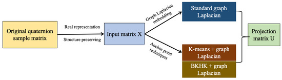
Figure 1. The overall workflow for dual graph Laplacian RPCA model with the anchor techniques.

Our proposed method for deriving the projection matrix U, as detailed in the flowchart shown in Figure 1, comprises three fundamental components. The processing pipeline begins with the encoding of input color images as pure quaternion matrices, and these matrices undergo an isomorphic transformation to their real representation, preserving the complete quaternion algebraic structure through block matrix representation. Subsequent dimensionality reduction is achieved through strategic extraction and vectorization of the principal column block, yielding the final data matrix. For the second component, we implement a sophisticated dual-graph framework through two methods. Among them, the KNN graph serves as a standard method for constructing the graph Laplacian matrix. In contrast, the anchor techniques we employ here, namely K-means and the BKHK method, function as acceleration strategies. Finally, the complete model is solved through the ADMM to obtain the projection matrix U, which will be elaborated upon later.

We employ the Augmented Lagrangian Multiplier (ALM) method to optimize the objective function. This approach reformulates the constrained optimization problem into a sequence of unconstrained subproblems by incorporating Lagrange multipliers and penalty terms. Through this iterative process, the method progressively converges towards the optimal solution. In the context of utilizing the ALM method to derive the optimal solution, we substitute Z for $U{V}^T+S$, and (26) can be equivalently reformulated as follows

$$\begin{array}{cc}\hfill \underset{U,V}{min}{\parallel X-Z\parallel }_F^2& +\gamma Tr\left(U^T{L}_{U}U\right)+\gamma Tr\left(V^T{L}_{V}V\right)+\lambda {\parallel S\parallel }_1,\hfill \\ & s.t.U^{T}U=I,Z=U{V}^T+S.\hfill \end{array}$$

(27)

According to the ALM method, (27) can be equivalently minimized as

$$\begin{array}{cc}\hfill L_{\mu ,\nu ,Y,\mathrm{\Gamma }}(S,Z,U,V)=& {\parallel X-Z\parallel }_F^2+\gamma Tr\left(U^T{L}_{U}U\right)+\gamma Tr\left(V^T{L}_{V}V\right)\hfill \\ & +{\lambda \parallel S\parallel }_1+Tr\left(Y^T(Z-U{V}^T-S)\right)+{\displaystyle \frac{\mu }{2}}{\parallel Z-U{V}^T-S\parallel }_F^2\hfill \\ & +Tr\left({\mathrm{\Gamma }}^T(U^{T}U-I)\right)+{\displaystyle \frac{\nu }{2}}{\parallel U^{T}U-I\parallel }_F^2,\hfill \end{array}$$

(28)

where $\mathrm{\Gamma }$ and $\mathrm{\Lambda }$ are Lagrange multipliers, and $\mu$ and $\nu$ are the step size in the update rule.

Given that there are four variables requiring solution, the Alternating Direction Method of Multipliers (ADMM) is employed to address this problem. It simplifies the solution process by allowing us to solve for a single variable while keeping the others fixed. By applying this method, the optimization problem represented by (28) can be naturally decomposed into four subproblems.

Problem 1.

With variables $U,V,Z$ fixed, the variable S is solved by rewriting (28)

$$L_{\mu ,\nu ,Y,\mathrm{\Gamma }}(S,Z,U,V)={\lambda \parallel S\parallel }_1+{\displaystyle \frac{\mu }{2}}{\parallel Z-U{V}^T-S+{\displaystyle \frac{Y}{\mu }}\parallel }_F^2.$$

(29)

Equation (29) can be solved by the proximal shrink operator denoted as follows

$$\begin{array}{cc}\hfill S^{k+1}& =\mathrm{s}\mathrm{o}\mathrm{f}\mathrm{t}(Z^{k+1}-U^{k+1}{V}^{k+1,T}+{\displaystyle \frac{Y^k}{\mu }},{\displaystyle \frac{\lambda }{\mu }}),\hfill \\ & \mathrm{s}\mathrm{o}\mathrm{f}\mathrm{t}(a,\tau )=\mathrm{s}\mathrm{i}\mathrm{g}\mathrm{n}\left(a\right) \mathrm{m}\mathrm{a}\mathrm{x}\left(\right|a|-\tau ,0).\hfill \end{array}$$

(30)

Problem 2.

With variables $V,S,Z$ fixed, the variable U is solved by rewriting (28)

$$\begin{array}{cc}\hfill L_{\mu ,\nu ,Y,\mathrm{\Gamma }}(S,Z,U,V)=& \gamma Tr\left(U^T{L}_{U}U\right)+Tr\left(Y^T(Z-U{V}^T-S)\right)\hfill \\ & +{\displaystyle \frac{\mu }{2}}\parallel Z-U{V}^T{-S\parallel }_F^2+Tr\left({\mathrm{\Gamma }}^T(U^{T}U-I)\right)+{\displaystyle \frac{\nu }{2}}{\parallel U^{T}U-I\parallel }_F^2,\hfill \end{array}$$

(31)

$$\begin{array}{cc}\hfill L=& \gamma Tr\left(U^T{L}_{U}U\right)-Tr\left(V^T{Y}^{T}U\right)-\mu Tr\left(Z^{T}U{V}^T\right)+{\displaystyle \frac{\mu }{2}}Tr\left(V{U}^{T}U{V}^T\right)\hfill \\ & +\mu Tr\left(V^T{S}^{T}U\right)+Tr\left({\mathrm{\Gamma }}^T{U}^{T}U\right)+{\displaystyle \frac{\nu }{2}}{\parallel U^{T}U-I\parallel }_F^2.\hfill \end{array}$$

(32)

By computing the partial derivative with respect to the variable U in (32), we obtain

$$\begin{array}{cc}\hfill {\displaystyle \frac{\partial L}{\partial U}}& =2\gamma L_{U}U-YV-\mu ZV+\mu U\left(V^{T}V\right)\hfill \\ & +\mu SV+2U\mathrm{\Gamma }+\nu (2U{U}^{T}U-U).\hfill \end{array}$$

(33)

By setting the Equation (33) equal to 0, the updated iteration formula for variable U can be addressed via the Sylvester equation, which takes the standard form $AX+XB=C$ where $X=U$ is the solution matrix, as showed below

$$\begin{array}{c}\hfill 2\gamma L_{U}U-YV-\mu ZV+\mu U\left(V^{T}V\right)+\mu SV+2U\mathrm{\Gamma }+\nu (2U{U}^{T}U-U)=0.\end{array}$$

(34)

$$(2\gamma L_U+\nu I)U+U(\mu V^{T}V+2\mathrm{\Gamma })=YV+\mu (Z-S)V.$$

(35)

Problem 3.

With variables $U,S,Z$ fixed, the variable V is solved by rewriting (28)

$$\begin{array}{cc}\hfill L_{\mu ,\nu ,Y,\mathrm{\Gamma }}(S,Z,U,V)=& \gamma Tr\left(V^T{L}_{V}V\right)+Tr\left(Y^T(Z-U{V}^T-S)\right)\hfill \\ & +{\displaystyle \frac{\mu }{2}}{\parallel Z-U{V}^T-S\parallel }_F^2,\hfill \end{array}$$

(36)

$$\begin{array}{cc}\hfill L=& \gamma Tr\left(V^T{L}_{V}V\right)-Tr\left(V^T{Y}^{T}U\right)-\mu Tr\left(Z^{T}U{V}^T\right)\hfill \\ & +{\displaystyle \frac{\mu }{2}}Tr\left(V{U}^{T}U{V}^T\right)+\mu Tr\left(V^T{S}^{T}U\right).\hfill \end{array}$$

(37)

Similar to the procedure outlined in (33), we derive the partial derivative of the variable U in Equation (37)

$$\begin{array}{cc}\hfill {\displaystyle \frac{\partial L}{\partial V}}& =2\gamma L_{V}V-Y^{T}U-\mu Z^{T}U+\mu V\left(U^{T}U\right)+\mu S^{T}U.\hfill \end{array}$$

(38)

The updated iteration formula for variable V also involves solving the Sylvester equation, which also takes the standard form $AX+XB=C$ where $X=V$ is the solution matrix, as detailed below

$$\begin{array}{c}\hfill 2\gamma L_{V}V-Y^{T}U-\mu Z^{T}U+\mu V\left(U^{T}U\right)+\mu S^{T}U=0\end{array}.$$

(39)

$$2\gamma L_{V}V+V\left(\mu U^{T}U\right)=Y^{T}U+\mu (Z^T-S^T)U.$$

(40)

Problem 4.

With variables $U,V,S$ fixed, the variable Z is solved by rewriting (28)

$$\begin{array}{c}\hfill L_{\mu ,\nu ,Y,\mathrm{\Gamma }}(S,Z,U,V)={\parallel X-Z\parallel }_F^2+{\displaystyle \frac{\mu }{2}}{\parallel Z-U{V}^T-S+{\displaystyle \frac{Y}{\mu }}\parallel }_F^2\end{array}.$$

(41)

The problem described by Equation (41) is convex, which facilitates a straightforward update of the variable Z as follows

$$Z^{k+1}={\displaystyle \frac{2X+\mu (U{V}^T+S-\frac{Y}{\mu })}{2+\mu }}.$$

(42)

Therefore, building upon the Augmented Lagrangian Method (ALM) and Alternating Direction Method of Multipliers (ADMM), we present the detailed optimization procedure in Algorithm 1.

Algorithm 1 The solution to optimize (26)

Require: Facial image data matrix: $X_{m\times n}$, Parameters: $k,r,\lambda ,\gamma ,\mu ,\nu$ Ensure: $U_{m\times k},V_{n\times k}$ 1: Initialize $Z,Y,S,U,V$ 2: repeat 3:    Update S by (30). 4:    Update U by (35). 5:    Update V by (40). 6:    Update Z by (42). 7:    Update Y by $Y^{r+1}=Y^r+{\mu }^r(Z^T-U{V}^T-S)$. 8:    Update $\mathrm{\Gamma }$ by ${\mathrm{\Gamma }}^{k+1}={\mathrm{\Gamma }}^k+\nu (U^{k+1,T}{U}^{k+1}-I)$. 9:    Update $\mu$ by ${\mu }^{r+1}=\rho {\mu }^r$. 10: until convergence

Having established the optimization framework, we next present a rigorous convergence analysis of our algorithm.

Theorem 1.

Under the following conditions:

1.

The graph Laplacian matrices $L_U,L_V$ are positive semi-definite,

2.

The iterative matrices $U^k\in {\mathbb{R}}^{m\times r}$ and $V^k\in {\mathbb{R}}^{n\times r}$ maintain full column rank,

3.

The parameters satisfy $\mu >0$, $\nu >{\displaystyle \frac{2\gamma \parallel L_U{\parallel }_2}{\mu }}$, and $\gamma >0$,

the proposed algorithm exhibits the following convergence properties:

1.

Monotonic decrease of the objective function:

$$L^{k+1}-L^k\le -\rho {\parallel {\mathrm{\Theta }}^{k+1}-{\mathrm{\Theta }}^k\parallel }_F^2.$$

(43)

where $\rho =min\left\{1+{\displaystyle \frac{\mu }{2}},{\displaystyle \frac{\mu }{2}},{\displaystyle \frac{{\alpha }_V}{2}},{\displaystyle \frac{{\alpha }_U}{2}}\right\}$, with ${\alpha }_V=2\gamma {\lambda }_{min}\left(L_V\right)+\mu {\sigma }_{min}^2\left(U^{k+1}\right)$ and ${\alpha }_U=2\gamma {\lambda }_{min}\left(L_U\right)+\mu {\sigma }_{min}^2\left(V^k\right)+\nu$.

2.

Convergence of primal variables:

$$\underset{k\to \infty }{lim}{\parallel {\mathrm{\Theta }}^{k+1}-{\mathrm{\Theta }}^k\parallel }_F=0.$$

(44)

3.

Convergence of Lagrangian multipliers:

$$\underset{k\to \infty }{lim}\parallel Y^{k+1}-Y^k{\parallel }_F=0,\underset{k\to \infty }{lim}{\parallel {\mathrm{\Gamma }}^{k+1}-{\mathrm{\Gamma }}^k\parallel }_F=0.$$

(45)

Proof. Part 1:

Monotonicity of the Objective Function

The difference in the Lagrangian can be decomposed as:

$$\begin{array}{cc}\hfill L^{k+1}-L^k=& \underset{{\mathrm{\Delta }}_Z}{\underbrace{L\left(Z^{k+1}\right)-L\left(Z^k\right)}}+\underset{{\mathrm{\Delta }}_S}{\underbrace{L\left(S^{k+1}\right)-L\left(S^k\right)}}\hfill \\ \hfill & +\underset{{\mathrm{\Delta }}_V}{\underbrace{L\left(V^{k+1}\right)-L\left(V^k\right)}}+\underset{{\mathrm{\Delta }}_U}{\underbrace{L\left(U^{k+1}\right)-L\left(U^k\right)}}.\hfill \end{array}$$

(46)

For each subproblem, we establish the following bounds:

• Z-subproblem:

  $${\mathrm{\Delta }}_Z=-\left(1+{\displaystyle \frac{\mu }{2}}\right){\parallel Z^{k+1}-Z^k\parallel }_F^2.$$

  (47)
• S-subproblem:

  $${\mathrm{\Delta }}_S\le -{\displaystyle \frac{\mu }{2}}{\parallel S^{k+1}-S^k\parallel }_F^2.$$

  (48)
• V-subproblem:

  $${\mathrm{\Delta }}_V\le -{\displaystyle \frac{1}{2}}\left(2\gamma {\lambda }_{min}\left(L_V\right)+\mu {\sigma }_{min}^2\left(U^{k+1}\right)\right){\parallel V^{k+1}-V^k\parallel }_F^2.$$

  (49)
• U-subproblem:

  $${\mathrm{\Delta }}_U\le -{\displaystyle \frac{1}{2}}\left(2\gamma {\lambda }_{min}\left(L_U\right)+\mu {\sigma }_{min}^2\left(V^k\right)+\nu \right){\parallel U^{k+1}-U^k\parallel }_F^2.$$

  (50)

Combining these bounds yields the monotonic decrease property in (43).

Part 2: Convergence of Primal Variables

Since the sequence $\left\{L^k\right\}$ is bounded below and monotonically decreasing, we have:

$$\sum _{k=0}^{\infty }{\parallel {\mathrm{\Theta }}^{k+1}-{\mathrm{\Theta }}^k\parallel }_F^2\le {\displaystyle \frac{L^0-L^{*}}{\rho }}<\infty .$$

(51)

which implies (44).

Part 3: Convergence of Lagrangian Multipliers

From the update rules:

$$\begin{array}{cc}\hfill \parallel Y^{k+1}-Y^k{\parallel }_F& =\mu \parallel (Z^{k+1}-U^{k+1}{V}^{k+1,\top }-S^{k+1})-(Z^k-U^k{V}^{k,\top }-S^k){\parallel }_F\hfill \\ \hfill & \le \mu \parallel {\mathrm{\Theta }}^{k+1}-{\mathrm{\Theta }}^k{\parallel }_F\to 0,\hfill \end{array}$$

and similarly for ${\mathrm{\Gamma }}^k$, establishing (45). □

4. Experiments

4.1. Datasets

The proposed model is rigorously evaluated on the Georgia Tech face dataset [33] and the VGG Face2 dataset [34]. The Georgia Tech face dataset serves as a well-controlled benchmark, containing facial images from 50 distinct subjects with 15 samples per subject, exhibiting carefully captured variations in lighting conditions, diverse facial expressions including neutral, smiling and surprised states, and head poses (e.g., frontal, side views). While the VGG Face2 dataset serves as a comprehensive large-scale benchmark, containing over 3 million facial images from more than 9000 distinct subjects, with each subject represented by an average of 300 samples exhibiting natural variations in real-world conditions. The dataset captures significant challenges including extreme pose variations, diverse facial expressions in uncontrolled environments, substantial variations in illumination conditions (both indoor and outdoor settings), and various types of occlusions (e.g., glasses, hair, hands). This diversity facilitates robust assessment of model generalization under challenging real-world conditions. We use 50 subjects from GT database and select 40 subjects from VGG Face2 dataset, where representative samples of GT database are visualized in Figure 2. All images in both database are preprocessed by manual cropping and resizing to a uniform resolution of $44\times 33$ pixels.

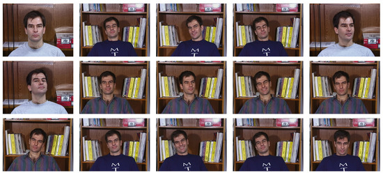
Figure 2. Sample images for one individual of the GTdatabase.

4.2. Parameter Selection

Our model involves six critical parameters: $\gamma$, $\lambda$, $\mu$, $\nu$, k and r, which must be carefully tuned in the formulation (28). The regularization parameters $\gamma =0.005$ and $\nu =0.001$ were determined via comprehensive sensitivity analysis, as shown in Figure 3. For the regularization parameters $\mu$ and $\lambda$, we adopt $\mu =0.005$ and $\lambda ={\displaystyle \frac{1}{\sqrt{max(m,n)}}}$ as suggested in [5,30]. Additionally, the parameter selection of k and r was carefully determined based on the dataset characteristics ($n=750$ samples, $d=5808$ features) and extensive empirical validation. For the graph construction, we set $k=15$ nearest neighbors, which represents approximately 2% of the total sample size. This proportion ensures adequate local structure representation while avoiding overfitting. Furthermore, considering the original dimensions, we respectively set $r=200$ and $r=100$ to compare the final results. These parameter choices are carefully calibrated to optimize the model’s performance across diverse scenarios.

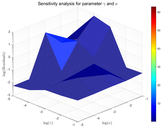
Figure 3. Sensitivity analysis for parameter $\gamma$ and $\nu$, where the residual is $\parallel X-U{V}^T{-S\parallel }_F^2$.

4.3. Experiment Results

Using the learned projection matrix U, we project the test samples into the low-dimensional space and compute their similarity to the training samples in this reduced space using Euclidean distance. This enables nearest neighbor classification, where recognition results are determined by identifying the closest matches based on similarity. To evaluate the model’s performance, we employ two metrics: the standard accuracy (ACC) and the convergence time. ACC measures the face matching accuracy, defined as the ratio of correctly classified samples to the total number of test samples, providing a quantitative assessment of the model’s recognition capability. Specifically, ACC is calculated as

$$ACC={\displaystyle \frac{{\sum }_{i=1}^n\sigma (p_i,map\left(q_i\right))}{n}}\times 100\%,$$

(52)

where $p_i$ is the predicted label of a test sample and $map\left(q_i\right)$ is the real label of the test sample. $\sigma (x,y)$ equals 1 if $x=y$ and 0 otherwise.

We partitioned the dataset into training and test sets with ratios of 0.7 and 0.8 corresponding to the GTdatabase and VGG Face2 dataset, respectively. To ensure statistical reliability and robustness, the results reported are the average values obtained from 10 independent trials, providing a more precise and representative assessment of the model’s performance.

For the $k=15$-nearest neighbors, we set the dimensionality reduction parameter to $r=200$. The corresponding accuracy and runtime of the model, evaluated using the original graph Laplacian matrix, the graph Laplacian matrix constructed via K-means, and the graph Laplacian matrix generated by the BKHK method, are summarized in Table 1.

Table 1. Results of RPCA with graph Laplacian constraint on GTdatabase (r = 200).

Method	Accuracy (%)	Running Time (s)	Notes
Standard graph Laplacian	73.8%	991.94	Baseline method
K-means + graph Laplacian	73.3%	935.39	K-means for anchor selection
BKHK + graph Laplacian	73.3%	973.15	BKHK for anchor selection

Similarly, for the $k=15$-nearest neighbors, we conducted an additional experiment with the dimensionality reduction parameter set to $r=100$. The accuracy and runtime of the model with original graph Laplacian matrix, graph Laplacian matrix constructed via K-means, and graph Laplacian matrix generated by the BKHK method are summarized in Table 2.

Table 2. Results of RPCA with graph Laplacian constraint on GTdatabase (r = 100).

Method	Accuracy (%)	Running Time (s)	Notes
Standard graph Laplacian	73.3%	2924.71	Baseline method
K-means + graph Laplacian	72.9%	2765.83	K-means for anchor selection
BKHK + graph Laplacian	72.9%	2132.40	BKHK for anchor selection

Additionally, we conducted the same experiments on VGG Face2 dataset and obtained the results at two dimensionality reduction settings ($r=100$ and $r=200$) as shown in Table 3 and Table 4:

Table 3. Results of RPCA with graph Laplacian constraint on VGG Face2 dataset ($r=200$).

Method	Accuracy (%)	Running Time (s)	Notes
Standard graph Laplacian	45.75	920.59	Baseline method
K-means + graph Laplacian	43.75	914.04	K-means for anchor selection
BKHK + graph Laplacian	43.75	844.23	BKHK for anchor selection

Table 4. Results of RPCA with graph Laplacian constraint on VGG Face2 dataset ($r=100$).

Method	Accuracy (%)	Running Time (s)	Notes
Standard graph Laplacian	45.0	921.32	Baseline method
K-means + graph Laplacian	42.5	896.81	K-means for anchor selection
BKHK + graph Laplacian	42.5	802.37	BKHK for anchor selection

The experimental results demonstrate that while the standard graph Laplacian method achieves marginally superior accuracy (0.5–0.9% higher on GTdatabase and comparable performance within ±0.25% on VGG Face2), the BKHK-based anchor approach offers significantly enhanced computational efficiency, achieving speedups of 12.9–27.1% across both datasets. Crucially, these computational improvements are attained with minimal accuracy degradation (maintaining 94–97% of the standard method’s recognition performance). The BKHK method’s superior scalability characteristics, evidenced by its more favorable computational complexity growth with increasing dataset size, make it particularly well-suited for large-scale face recognition applications where processing efficiency is critical. These findings collectively demonstrate that the BKHK approach provides an optimal balance between recognition accuracy and computational efficiency, offering a practical solution for real-world deployment scenarios that demand both high performance and scalability. 

5. Conclusions

In this study, we present an advanced RPCA framework incorporating bidirectional graph Laplacian constraints and an anchor point strategy, achieving enhanced computational efficiency while preserving recognition accuracy in facial analysis. The dual-graph architecture captures intrinsic geometric relationships from both sample and feature perspectives, maintaining structural and discriminative characteristics of high-dimensional data. The anchor point techniques serves as a core component of this paper, where anchor points are selected as referrence sample points to efficiently construct the similarity matrix. In this regard, this paper compares the accuracy of several different anchor technologies in face recognition. To verify the reliability of the algorithm, a convergence analysis is also provided in this paper. Finally, extensive experiments on the GTdatabase and VGG Face2 dataset demonstrate superior processing speed and sustained accuracy under challenging conditions including illumination variations, expressions, and pose changes. While the anchor point strategy effectively reduces computational complexity with minimal accuracy loss, several limitations warrant consideration regarding sensitivity to anchor selection in non-uniform data distributions, memory overhead from graph matrix storage, and performance degradation when handling extreme occlusions. These challenges motivate three key future directions: developing scalable network architectures through dynamic anchor selection and adaptive graph sparsification, optimizing real-time execution capabilities via hardware-aware parallel computing strategies, and extending the framework to broader computer vision objectives such as video-based action recognition and 3D object analysis. Beyond facial analysis, the framework’s core methodology shows potential for extension to other domains involving high-dimensional data with underlying geometric structure, such as medical image analysis and multimodal sensor fusion applications. Future work will focus on developing dynamic graph learning capabilities for video-based recognition systems and exploring quantum computing adaptations to address fundamental complexity challenges, potentially opening new possibilities for large-scale pattern recognition systems.

References

- Kirby, M.; Sirovich, L. Application of the Karhunen-Loeve procedure for the characterization of human faces. IEEE Trans. Pattern Anal. Mach. Intell. 1990, 12, 103–108. [Google Scholar]
- Turk, M.; Pentland, A. Eigenfaces for recognition. J. Cognit. Neurosci. 1991, 3, 71–86. [Google Scholar]
- Yang, J.; Zhang, D.; Frangi, A.F.; Yang, J.Y. Two-dimensional PCA: A new approach to appearance-based face representation and recognition. IEEE Trans. Pattern Anal. Mach. Intell. 2004, 26, 131–137. [Google Scholar] [PubMed]
- Torres, L.; Reutter, J.Y.; Lorente, L. The importance of the color information in face recognition. In Proceedings of the 1999 International Conference on Image Processing (Cat. 99CH36348), Kobe, Japan, 24–28 October 1999; Volume 3, pp. 627–631. [Google Scholar]
- Yang, J.; Liu, C. A general discriminant model for color face recognition. In Proceedings of the IEEE 11th International Conference on Computer Vision, Rio de Janeiro, Brazil, 14–21 October 2007; pp. 1–6. [Google Scholar]
- Xiang, X.; Yang, J.; Chen, Q. Color face recognition by PCA-like approach. Neurocomputing 2015, 228, 231–235. [Google Scholar]
- Zhu, Y.; Zhu, C.; Li, X. Improved principal component analysis and linear regression classification for face recognition. Signal Process. 2018, 145, 175–182. [Google Scholar]
- Wright, J.; Ganesh, A.; Rao, S.; Peng, Y.; Ma, Y. Robust Principal Component Analysis: Exact Recovery of Corrupted Low-rank Matrices via Convex Optimization. Adv. Neural Inf. Process. Syst.s 2009, 22, 2080–2088. [Google Scholar]
- Candès, E.J.; Li, X.; Ma, Y.; Wright, J. Robust principal component analysis. J. ACM 2009, 58, 1–37. [Google Scholar]
- Wright, J.; Ma, Y. Dense error correction via l1-minimization. lEEE Trans. Inf. Theory 2010, 56, 3540–3560. [Google Scholar]
- Zhou, T.; Tao, D. Greedy Bilateral Sketch, Completion & Smoothing. In Artificial Intelligence and Statistics; PMLR: Birmingham, UK, 2013; Volume 31, pp. 650–658. [Google Scholar]
- Le Bihan, N.; Sangwine, S.J. Quaternion principal component analysis of color images. In Proceedings of the 2003 International Conference on Image Processing (Cat. No.03CH37429), Barcelona, Spain, 14–17 September 2003; pp. 809–812. [Google Scholar]
- Jia, Z. The Eigenvalue Problem of Quaternion Matrix: Structure-Preserving Algorithms and Applications; Science Press: Beijing, China, 2019. [Google Scholar]
- Denis, P.; Carre, P.; Fernandez-Maloigne, C. Spatial and spectral quaternionic approaches for colour images. Comput. Vis. Image Understand. 2007, 107, 74–87. [Google Scholar]
- Shi, L.; Funt, B. Quaternion color texture segmentation. Comput. Vis. Image Understand. 2007, 107, 88–96. [Google Scholar]
- Zou, C.; Kou, K.I.; Wang, Y. Quaternion collaborative and sparse representation with application to color face recognition. IEEE Trans. Image Process. 2016, 25, 3287–3302. [Google Scholar]
- Xiao, X.; Chen, Y.; Gong, Y.J.; Zhou, Y. 2D quaternion sparse discriminant analysis. IEEE Trans. Image Process. 2020, 29, 2271–2286. [Google Scholar]
- Chen, Y.; Xiao, X.; Zhou, Y. Low-rank quaternion approximation for color image processing. IEEE Trans. Image Process. 2020, 29, 1426–1439. [Google Scholar]
- Wang, Q.W.; Xie, L.M.; Gao, Z.H. A Survey on Solving the Matrix Equation AXB = C with Applications. Mathematics 2025, 13, 450. [Google Scholar] [CrossRef]
- Jia, Z.R.; Wang, Q.W. The General Solution to a System of Tensor Equations over the Split Quaternion Algebra with Applications. Mathematics 2025, 13, 644. [Google Scholar] [CrossRef]
- Cai, D.; He, X.F.; Han, J.W.; Huang, T.S. Graph regularized nonnegative matrix factorization for data representation. IEEE Trans. Pattern Anal. Mach. Intell. 2011, 33, 1548–1560. [Google Scholar]
- Jiang, B.; Ding, C.; Luo, B.; Tang, J. Graph-laplacian PCA: Closed-form solution and robustness. In Proceedings of the IEEE Conference on Computer Vision and Pattern Recognition, Portland, OR, USA, 25–27 June 2013. [Google Scholar]
- Feng, C.; Gao, Y.L.; Liu, J.X.; Zheng, C.H.; Yu, J. PCA based on graph laplacian regularization and P-norm for gene selection and clustering. IEEE Trans. Nanobiosci. 2017, 16, 257–265. [Google Scholar]
- Liu, J.X.; Wang, D.; Gao, Y.L.; Zheng, C.H.; Shang, J.L.; Liu, F.; Xu, Y. A joint-L2,1-norm-constraint-based semi-supervised feature extraction for RNA Seq data analysis. Neurocomputing 2017, 228, 263–269. [Google Scholar]
- Wang, J.; Liu, J.X.; Kong, X.Z.; Yuan, S.S.; Dai, L.Y. Laplacian regularized low-rank representation for cancer samples clustering. Comput. Biol. Chem. 2019, 78, 504–509. [Google Scholar]
- Yang, N.Y.; Duan, X.F.; Li, C.M.; Wang, Q.W. A new algorithm for solving a class of matrix optimization problem arising in unsupervised feature selection. Numer. Algorithms 2024. [Google Scholar] [CrossRef]
- Hamilton, W.R. Lectures on Quaternions. In Landmark Writings in Western Mathematics 1640–1940; Hodges and Smith: Dublin, Ireland, 1853. [Google Scholar]
- Jiang, T. Algebraic methods for diagonalization of a quaternion matrix in quaternionic quantum theory. J. Math. Phys. 2005, 46, 052106. [Google Scholar]
- Ding, L.; Li, C.; Jin, D.; Ding, S.F. Survey of spectral clustering based on graph theory. Pattern Recognit. 2024, 151, 110366. [Google Scholar]
- Kong, X.Z.; Song, Y.; Liu, J.X.; Zheng, C.H.; Yuan, S.S.; Wang, J.; Dai, L.Y. Joint Lp-Norm and L2,1-Norm Constrained Graph Laplacian PCA for Robust Tumor Sample Clustering and Gene Network Module Discovery. Front. Genet. 2021, 12, 621317. [Google Scholar]
- Zhao, H. Design and Implementation of an Improved K-Means Clustering algorithm. Mob. Inf. Syst. 2022, 2022, 6041484. [Google Scholar] [CrossRef]
- Gao, C.H.; Chen, W.Z.; Nie, F.P.; Yu, W.Z.; Wang, Z.H. Spectral clustering with linear embedding: A discrete clustering method for large-scale data. Pattern Recognit. 2024, 151, 110396. [Google Scholar]
- The Georgia Tech Face Database. Available online: http://www.anefian.com/research/face_reco.htm (accessed on 15 February 2025).
- The VGG Face2 Dataset. Available online: https://www.robots.ox.ac.uk/~vgg/data/vgg_face2/ (accessed on 15 February 2025).
Disclaimer/Publisher’s Note: The statements, opinions and data contained in all publications are solely those of the individual author(s) and contributor(s) and not of MDPI and/or the editor(s). MDPI and/or the editor(s) disclaim responsibility for any injury to people or property resulting from any ideas, methods, instructions or products referred to in the content. |
© 2025 by the authors. Licensee MDPI, Basel, Switzerland. This article is an open access article distributed under the terms and conditions of the Creative Commons Attribution (CC BY) license (https://creativecommons.org/licenses/by/4.0/).