Abstract
The digital twin model, which serves as a virtual counterpart symmetric to the physical entity, enables high-fidelity simulation and real-time monitoring. However, digital twin implementation for marine steam turbines (MSTs) faces dual multi-domain simulation fidelity and computational efficiency challenges. This study establishes a MST digital twin modeling methodology through two interconnected innovations: (1) a Modelica-based modular architecture enabling cross-domain coupling across mechanical, thermodynamic, and hydrodynamic systems via hierarchical decomposition, ensuring bidirectional symmetry between physical components and their virtual representations; and (2) a hybrid support vector regression-bidirectional long short-term memory (SVR-BiLSTM) surrogate model combining Gaussian radial basis function-supported SVR for steady-state mapping with Bi-LSTM networks for dynamic error compensation. Experimental validation demonstrates: (a) the SVR component achieves <1.57% absolute error under step-load conditions with 85% computational time reduction versus physics-based models; and (b) Bi-LSTM integration improves transient prediction accuracy by 14.85% in maximum absolute error compared to standalone SVR, effectively resolving static–dynamic discrepancies in telemetry simulation. This dual-approach innovation successfully bridges the critical trade-off between real-time computation and predictive accuracy while maintaining symmetric consistency between the physical turbine and its digital counterpart, providing a validated technical foundation for the intelligent operation and maintenance of MSTs.
1. Introduction
Under the intelligent and digital transformation of maritime systems, developing high-fidelity digital twins for marine steam turbines (MSTs) has become a crucial technology to enhance ship safety and operational efficiency [1,2]. By establishing precise digital mappings of dynamic physical systems, high-fidelity digital twins provide crucial data infrastructure for fault diagnosis and health management [3,4]. Grounded in the digital twin concept proposed by Grieves and Vickers [5], its technological essence lies in integrating high-fidelity simulation models with real-time sensor data to create dynamic virtual replicas of physical assets [6,7]. The physics-based model data integrated digital twin modeling technique addresses limitations inherent in conventional monitoring approaches, thus underscoring the technical urgency of constructing high-credibility digital twins for marine steam turbine systems [8]. Digital twin technologies enable multisource data fusion and real-time decision-making for complex systems [9], integrating physics-informed simulations, sensor networks, and traceability frameworks to achieve prognostics via life prediction models [10], predictive maintenance through early fault detection, and dynamic positioning analytics for MSTs. The digital twin architecture for MST systems is illustrated in Figure 1.
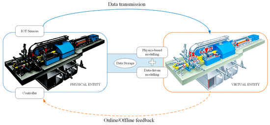
Figure 1.
Conceptual diagram of digital twin modeling of a MST system.
Although digital twin technology has attained operational maturity in broader industrial contexts, unresolved technical trade-offs challenge its deployment for MSTs [11,12]. Mrzljak et al. [13] analyzed the energy efficiency and performance of LNG carriers’ main feedwater pump systems, including turbo-generators and steam turbines, exploring optimization strategies in energy conversion processes. Yu et al. [14] developed a real-time online performance monitoring system for steam turbine generators using a digital twin model to optimize operational efficiency and control capabilities. Zhang et al. [15] investigated the characteristics and influencing factors of marine nuclear steam turbine units under coupling off-design conditions. Sun et al. [16] numerically simulated the steam flow excitation characteristics and control phase coverage relationships in marine steam turbine generator units. Nirbito et al. [17] introduced an improved compressor curve-based compound-cycle propulsion system for LNG ships, achieving a system efficiency of 48.49% and higher power output under full load. Dulau and Bica [18] developed a simulation framework for steam turbines using Continuity Equation and MATLAB/Simulink, achieving optimized performance and accurate predictions while acknowledging limitations in steam assumptions and computational complexity. Crucially, contemporary digital twin implementations for marine power generation systems reveal an intractable precision-efficiency dichotomy [19,20].
Current research on marine power systems has prioritized component-level analysis through advanced modeling techniques and dynamic performance evaluation. In contrast, systematic exploration of multi-domain coordination mechanisms and dynamic interaction patterns among thermal equipment remains underdeveloped. Recent advancements in multi-domain digital twin modeling methodologies have yielded diversified technical approaches [21,22]. Ding et al. [23] presented a Modelica-based thermal-hydraulic model for a helically coiled tube once-through steam generator (H-OTSG) based on the comprehensive analysis of empirical data and correlations. Suk King et al. [24] summarized the development and validation of a Modelica-based model for H-OTSGs, incorporating empirical data to simulate steady-state and transient performances accurately. Chetan et al. [6] developed a multi-fidelity digital twin-based structural model for downwind wind turbine rotor blades, which was validated through full-scale structural testing. Belli et al. [25] optimized a 75 kW and 155 kW double-fed induction generators, highlighting performance improvements and challenges in design and implementation for naval applications. Yang et al. [26] discussed ship steam power system performance simulation with rapid load changes using MMS software (version 5.0.0), highlighting impacts on efficiency and optimization strategies. At the same time, Zeng et al. [27] developed a Modelica-based digital twin model for multi-domain analysis of marine steam power systems, investigating dynamic characteristics and response rates under various operational conditions, with model accuracy verified through fault simulation scenarios. Zhang and Xu [28] introduced an unsupervised steam turbine engine anomaly detection method using an Enhanced LSTM Variational Autoencoder (ELSTMVAE), surpassing traditional LSTM and Improved VAE (ILVAE) approaches in accuracy, latency frame rate, and computational efficiency. Zhu et al. [29] used Modelica to develop high-fidelity models for a boiler system, achieving accurate dynamic responses and enhanced precision through parameter optimization. Cai et al. [30] optimized a support vector regression (SVR) model to systematically investigate building energy consumption prediction, demonstrating its strong performance across multiple aspects. Wang et al. [31] proposed a TREE-LSTM-driven model for variable-load fault detection, complemented by multi-physics coupling frameworks encompassing mechanical, thermodynamic, and hydrodynamic domains for comprehensive virtual replica construction, and physics-reduced surrogates, demonstrating well-documented accuracy–efficiency trade-offs [30,32,33].
However, critical gaps persist in current digital twin implementations. Schirmann [34] highlighted the development of physics-informed data-driven models for improving ship motion response predictions using global wave data. Kim et al. [35] developed a Modelica-driven digital twin framework to optimize nuclear-renewable hybrid systems, demonstrating that integrated storage-hydrogen tech boosts efficiency while showing computational trade-offs. Asgari et al. [36] presented a hybrid surrogate model for enhancing online temperature and pressure predictions in data centers through integrated thermal and pressure modeling. Lim et al. [37] presented a hybrid surrogate modeling framework for advancing digital twin applications in fluoride-salt-cooled high-temperature reactor design and safety analysis by integrating machine learning, physical modeling, and enhancing efficiency and accuracy. Kozlovska et al. [38] highlighted how integrating building energy management systems and building information modeling to enhance energy efficiency and sustainability in building design and operation. A Modelica-based thermoelectric co-generation model was presented to demonstrate that field-method electrical modeling achieves superior flexibility over nodal approaches, albeit with amplified algebraic constraints and computational costs [39].
Nevertheless, prevailing methodologies [24,25,26,27,28] exhibit two fundamental limitations: (1) fragmented multi-domain integration, where models operate through compartmentalized physical domain representations, compromising system-level fidelity through insufficient mechanical-thermal-fluid dynamic interactions; and (2) accuracy–efficiency paradox, as computational acceleration techniques inevitably sacrifice modeling precision through either data-driven approximations or physical simplification processes, as shown in Table 1.

Table 1.
Summary of existing digital twins of steam turbines.
To overcome these limitations, this work presents a dual-methodological framework for MST digital twins, addressing multi-domain coupling complexity through: (1) a Modelica-based modular architecture that enables hierarchical cross-domain interaction among mechanical, thermodynamic, and hydrodynamic subsystems via bidirectional symmetry, eliminating manual equation integration while preserving physical–virtual component consistency; and (2) a physics-guided SVR-BiLSTM hybrid surrogate that synergizes data-driven transient compensation with high-fidelity steady-state modeling, resolving static–dynamic discrepancies through complementary integration of physical constraints and adaptive error correction. Collectively, this approach establishes a computational paradigm that balances real-time efficiency with simulation fidelity, enabling intelligent operational decision-making for MSTs without compromising system complexity.
The remainder of this paper is organized as follows. Section 2 establishes operational principles and a mathematical modeling framework for MSTs. Section 3 develops a hybrid SVR-BiLSTM surrogate modeling methodology integrating steady-state mapping and dynamic error compensation. Section 4 validates model performance through comprehensive experimental studies. Section 5 concludes the research and outlines future directions.
2. System Modeling Framework for Marine Steam Turbines
2.1. Operational Mechanism of Marine Steam Turbines
The marine steam turbine generator set, comprising a steam turbine, regulating valves, condenser, and generator [15,27], is the core unit of ship power systems. Its operation follows a closed-loop energy cascade cycle: high-temperature, high-pressure (HP) steam first expands in the HP turbine, converting thermal energy into mechanical energy through blade rotation while progressively reducing pressure and temperature. The depressurized steam then undergoes secondary expansion in the low-pressure (LP) turbine to extract residual energy, enhancing overall efficiency [40]. The mechanical energy drives the generator to produce electricity for onboard equipment, with a speed-regulating mechanism dynamically adjusting steam flow to stabilize rotational speed and ensure continuous power output during load fluctuations. Exhaust steam from the LP turbine is condensed into liquid via seawater cooling in the condenser, then recirculated by pumps to boilers for reheating, forming a closed-loop working fluid cycle that maximizes resource regeneration. Mathematical models balancing accuracy and computational efficiency must be developed to characterize system dynamics, incorporating multidimensional coupling analyses of turbine expansion processes, condenser heat exchange efficiency, and generator electromagnetic characteristics (as shown in Figure 2), thereby enabling operational optimization and fault diagnosis.
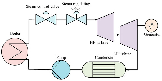
Figure 2.
Working principle of a marine steam turbine generator set.
2.2. Multi-Physics Mathematical Modeling
This research develops a mathematical model for marine steam turbine generator systems using a Modelica-based multidisciplinary modeling approach. Modelica, an equation-based object-oriented modeling language developed by the Modelica Association, is a non-proprietary open standard widely adopted in mechanical, electrical, hydraulic, thermal, and control engineering. The methodology is implemented through MWORKS, a Modelica-compliant platform developed by Suzhou Tongyuan, to construct a high-fidelity physics-based MST system model, as shown in Figure 3. The framework employs a dual-dimensional architecture integrating vertical stratification and horizontal modularization to achieve precise virtual–physical system alignment. Vertically, it resolves multi-domain coupling effects across mechanical, electrical, and thermodynamic subsystems. Horizontally, critical components such as steam boilers, turbines, and generators are decomposed into parameterized modules interconnected via standardized interfaces. This hierarchical modular design enables subsystem-level optimization while preserving system-level fidelity in digital twin applications, effectively balancing localized refinement with global operational accuracy.
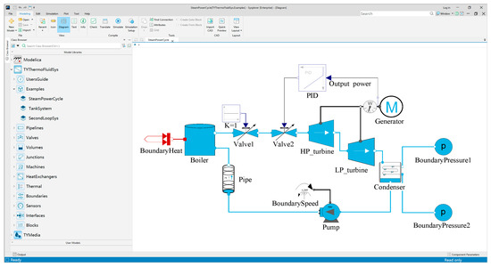
Figure 3.
System model of the steam turbine generator based on MWORKS, a Modelica-compliant multi-domain system modeling platform.
To conduct an accurate thermodynamic analysis of the marine steam turbine generator, it is necessary to establish a detailed mathematical model. Here, this paper primarily describes the mathematical models of the main steam turbine and the regulating valve.
2.2.1. Thermodynamic Modeling of the Main Steam Turbine
The thermodynamic analysis of steam turbines primarily involves analyzing and calculating their operating conditions under both rated and variable conditions, as well as determining the inlet and outlet flow rates and output power based on design specifications [41]. The steam flow is calculated indirectly from turbine regulation stage pressure and temperature. The turbine converts high-pressure steam energy into mechanical work via blade rotation. The inlet steam flow rate can be expressed by the following formula:
where and are the steam flow rates at the turbine inlet during the dynamic process and design condition, respectively, and are the inlet pressures of the turbine during the dynamic process and under the design condition, respectively, and are the steam temperatures at the turbine inlet during the dynamic process and design condition, respectively, is the correction coefficient, is the rotation angle of the trip valve cam, and is the fitting factor.
According to relevant theories in engineering mechanics, when steam performs work within the turbine without an increase in entropy, the process is considered an isentropic expansion process, during which the shaft work is maximized:
where and are entropy values of the steam at the turbine inlet and outlet, respectively, is the enthalpy value at the turbine inlet during isentropic expansion, and is the enthalpy value at the turbine outlet during the isentropic expansion process.
Based on the work value of evaporation and expansion during the isentropic process and the efficiency of the turbine, the actual shaft work output of the turbine and the enthalpy value of the steam at the outlet can be obtained by
where is the actual outlet enthalpy value of the steam, is the relative internal efficiency; is the mechanical efficiency, and is the actual shaft work output.
The rotor dynamics equation is:
where is the moment of inertia, is the angular velocity of the rotor, is the output torque, and is the output torque.
2.2.2. Dynamic Modeling of the Control Valve System
The inlet valve of the steam turbine generator set is one of the primary control objects for large disturbances in the power system. By adjusting the valve, the inlet flow rate of the turbine generator set and the user power output can be regulated and controlled. The mathematical expression for the relationship between its opening degree and flow rate is as follows:
where R is the valve adjustability ratio, which is the ratio of the maximum flow rate to the minimum flow rate that the valve can regulate.
Based on the valve flow formula and the relationship between valve flow and the flow coefficient:
where is the flow coefficient of the valve, is the flow coefficient of the valve at its maximum opening, P is the pressure difference across the valve, and is the density of the medium flowing through the valve.
By substituting Equations (9) and (10) into Equation (8), the relationship between the linear valve flow, valve opening, and pressure across the valve can be obtained as follows:
In this paper, the control of equipment in the system is mainly controlled by PID, and its control equation is as follows:
where is difference between the set value and the actual value, is the scaling factor, is the integration coefficient, and is the differential coefficient.
All state parameters are nondimensionalized based on their design data. The formula is
where is the dimensionless parameter, is the simulation or experimental parameter, and is the design parameter.
3. Hybrid SVR-BiLSTM Surrogate Modeling Methodology
The construction of MSTs is based on multi-stage fluid dynamics theory, achieving coupling of fluid interfaces across stages through mass, momentum, and energy conservation equations. However, cross-domain iterative solving of these equations results in high computational complexity, causing significant degradation in real-time model performance, which constitutes the fundamental bottleneck of this methodology. Concurrently, the model’s reliance on operation-condition-dependent empirical coefficients and its unmodeled deficiencies in dynamic characteristics, such as transient nonlinear responses, lead to systematic deviations between the physics-based model and actual operational behaviors of MSTs. These deviations impair state prediction accuracy during operational mode transitions, critically affecting maintenance phases. To overcome the dual challenges, e.g., real-time performance versus fidelity, in digital twin modeling of MSTs, this study proposes a hierarchical surrogate modeling framework optimized through three-phase system integration, as shown in Figure 4: Phase I develops a steady-state surrogate model guided by orthogonal experimental design under physical constraints, achieving full parameter space coverage. Its simulation dataset provides training foundations for machine learning algorithms to characterize turbine static operations precisely. Phase II addresses transient prediction errors through residual analysis between dynamic test data and steady-state outputs, employing deep learning time-series algorithms to establish dynamic compensation models that enhance adaptability to rapid operational changes. Finally, the cascaded integration of steady-state and dynamic compensation models resolves the traditional trade-off between real-time performance and dynamic fidelity.
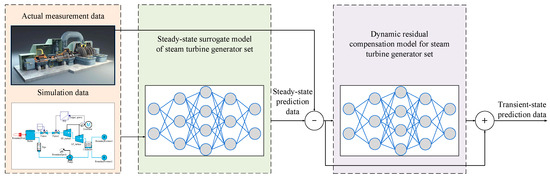
Figure 4.
Schematic diagram of the application process for the MST surrogate model.
3.1. Steady-State Surrogate Model Development
This study constructs a variable-condition physics-based steady-state surrogate model using SVR, systematically characterizing the static characteristics of steam turbines across wide operational ranges through full-parameter-space sampling strategies. The modeling layer establishes a high-confidence static characteristic benchmark, with its core value lying in providing rigorous precision boundaries for dynamic compensation models via error-controlled steady-state predictive capability. Implementation involves training SVR algorithms with multi-dimensional datasets generated by variable-condition physics-based models, developing lightweight surrogate models with rapid response capabilities while ensuring nonlinear mapping accuracy and achieving a quantum leap in computational efficiency.
3.1.1. SVR Algorithm Design
SVR is a classical regression algorithm based on SVM theory and has been widely applied in regression analysis [23]. When the sample size is limited and the input–output feature dimensions are relatively low, SVR utilizes kernel functions to map original data into a high-dimensional space, transforming nonlinear problems in low-dimensional space into linear ones in high-dimensional space, thereby obtaining more complex decision boundaries.
In the high-dimensional feature space, SVR achieves prediction by solving for the optimal regression hyperplane, minimizing the distance between samples and the hyperplane. Simultaneously, slack variables are introduced to balance model complexity and the influence of outliers, thereby enhancing the model’s generalization ability and robustness. Based on these principles, this study employs SVR to construct a surrogate model for the turbine’s steady-state performance. The specific steps are as follows:
where is the input value, and is the output target value. The regression estimation function for SVR is expressed as:
where is the weight vector, is the bias constant, and x is the input eigenvector.
According to the theory of mathematical statistics, the function estimation problem can be transformed into the optimization problems expressed in Equations (17) and (18):
where is the insensitivity loss factor, which represents the maximum allowable deviation for the samples.
Since individual data points cannot be accurately estimated within the precision of , slack variables and are introduced. Based on the strategy of structural risk minimization, the optimization problem is reformulated as:
where C is the penalty factor, and N is the number of datasets. To facilitate solving, the optimization problem can be transformed into a dual-variable optimization problem using Lagrange duality. That is, the optimal solution to the original problem can be obtained by solving the equivalent dual problem. By introducing Lagrange multipliers and , the model is transformed into its dual problem, and the final expression for the corresponding linear regression function is obtained as:
By introducing the kernel function to replace the vector inner product, the linear problem is transformed into a nonlinear regression problem in Hilbert space, and the SVR model is constructed as:
Finally, are the optimal solutions, and the corresponding function expression is:
The most commonly used kernel function is the radial basis function (RBF) kernel (also known as the Gaussian kernel function), which is expressed as:
where is the kernel width.
3.1.2. SVR-Based Steady-State Model Implementation
This section describes the process of generating a large sample dataset through batch physics-based model simulations and training the steady-state surrogate model. First, the physics-based model constructed in the previous section is used to simulate the turbine unit under various operating conditions, generating the training dataset. The SVR algorithm is then applied to train the data, utilizing kernel functions to map the data into a high-dimensional space, addressing the nonlinear regression issues among multiple parameters. This method ensures robustness even with a small dataset. The hyperparameters of the SVR algorithm are optimized using a grid search strategy, ultimately yielding a steady-state surrogate model for the turbine unit driven by the physics-based model. The main workflow for constructing the steady-state surrogate model is as shown in Figure 5.
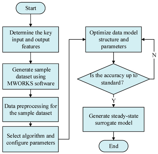
Figure 5.
Training process of the turbine steady-state surrogate model.
Step 1: Define the input and output of the surrogate model. Based on expert knowledge, key feature parameters are selected from the turbine physics-based simulation model to serve as the input parameters for the surrogate model. These include inlet steam temperature, inlet steam pressure, exhaust pressure, and rotational speed. The output parameters consist of critical variables and some latent data, such as inter-stage pressure, flow rate, and internal power at each stage.
Step 2: Generate training data in batches using the model experiment toolbox in MWORKS. Based on the turbine physics-based model established in the previous sections, the orthogonal experimental design and batch simulation capabilities of the model experiment toolbox in MWORKS are utilized. This facilitates the generation of training sample data for the surrogate model. By leveraging the convenient features of the toolbox, a comprehensive set of training data is constructed, capturing the behavior of the turbine under various operating conditions through systematic and efficient simulations. The resulting dataset serves as the foundation for subsequent training processes.
Step 3: Data preprocessing of sample data. The sample data obtained from the previous step are preprocessed to improve their quality and suitability for training. Perform max–min normalization on both input and output features to eliminate dimensional differences between them, then divide the preprocessed dataset into a training set and a testing set in an 8:2 ratio. Randomly shuffle the samples within both the training and testing sets to remove any inherent order in the data that could introduce bias during training or testing.
Step 4: Algorithm selection and configuration. When the SVR algorithm is selected for model training, randomly initialize the algorithm’s initial weight parameters, restricting the initial weights within the range [0, 1]. Compute the outputs of each layer based on these initial weights. Then, set the allowable iterative error ε = 1 × 10⁻⁵, limit the maximum number of iterations to 5000, and set the initial learning rate to 0.003.
Step 5: Model training and error calculation. Calculate the error values for each node in the output layer, denoted as , and compute the total error energy . Check whether the number of samples that have been learned has reached the total number of samples in the training set. If not, return to step 3; otherwise, proceed to the next step.
Step 6: Accuracy evaluation. If the total error energy of the samples , or if the maximum number of iterations has been reached, proceed to Step 8. Otherwise, move to the next step.
Step 7: Model weight parameter. An optimization algorithm is employed to optimize and update the parameters of the kernel function until a hyperplane that satisfies the fitting conditions is found.
Step 8: End of training. Obtain the turbine steady-state surrogate model that satisfies the required accuracy.
3.2. Dynamic Error Compensation Model Construction
Steady-state turbine models exhibit predictive deviations under transient conditions due to dynamic characteristics and nonlinear time-varying relationships. To address this, a transient error-correction surrogate model is developed, leveraging time-series analysis of dynamic test data to capture nonlinear dynamic features and compensate for prediction errors. Serving as a complement to steady-state models, this framework specifically addresses transient prediction limitations [24], maintaining accuracy during rapid operational transitions while enhancing overall system reliability and adaptability.
3.2.1. Bi-LSTM Prediction Framework
LSTM consists of multiple recurrent units, among which the memory cell is the core component responsible for storing and maintaining information. The memory cell dynamically updates its content based on changes in the input and the current state. There are three gating mechanisms in LSTM: the input gate (), the forget gate (), and the output gate (). Through these mechanisms, LSTM effectively manages the flow of information across time steps, enabling it to capture long-term dependencies in sequential data. By combining these three gating mechanisms, the update process of LSTM can be described as follows:
Input Gate:
Forget Gate:
Memory Cell:
Output Gate:
Output features:
In the equations, t and t − 1 denote the current and previous time steps, respectively, while tanh are activation functions and represent the input feature data at the current time step. represents the memory cell state from the previous time step. represents the hidden state (output information) from the previous time step, which encapsulates information from earlier time steps. W denotes the weight matrices, b denotes the bias vectors, and represents element-wise multiplication (not convolution). and tanh are activation functions.
Bi-LSTM is constructed by combining two LSTMs that operate in opposite directions, allowing it to extract and combine information from both the forward and backward directions of sequential data [13]. This bidirectional information extraction enriches the learned representations, enabling the network to better capture long-term dependencies in time-series data. By processing data in both temporal directions, the Bi-LSTM enhances the network’s ability to learn from long sequences, improves data utilization, and increases prediction accuracy while effectively reducing the risk of underfitting. The structure of the Bi-LSTM network is illustrated in Figure 6.
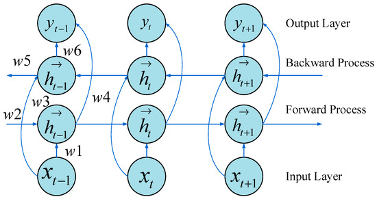
Figure 6.
Structure of the Bi-LSTM network.
As shown in Figure 6, when the output is influenced by both the forward layer and the backward layer, the output takes the following form:
where represents the weight matrix, denotes the output of the forward hidden layer, and denotes the output of the backward hidden layer.
3.2.2. Time-Series Error Correction Model Integration
The surrogate model of MSTs trained using sampling data based on the physics-based model is essentially a steady-state condition model. However, since physics-based models struggle to describe the dynamic characteristics of the unit during transient conditions, there will inevitably be prediction deviations when applying this model to variable working conditions. Since variable working conditions represent a continuous process, a time-series prediction algorithm is adopted to construct the error correction model. Considering that the turbine’s thermodynamic performance parameters are influenced by both short-term and long-term historical states, the Bi-LSTM algorithm is suitable for effectively modeling these long- and short-term sequence data. The procedure is as shown in Figure 7.
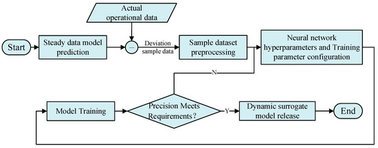
Figure 7.
Error correction model construction using the Bi-LSTM model.
The input features of the Bi-LSTM neural network error compensation model are the input features of the surrogate model, and the output is the deviation between the surrogate model’s output and the experimental results. The input and output features are preprocessed using min–max scaler normalization to eliminate the dimensional differences between features. The entire dataset is first randomly shuffled and then divided into a training set and a test set in a ratio of 0.8:0.2. The training set is used to train the error compensation model, while the test set is used to evaluate the accuracy of the error model. The hyperparameters of the Bi-LSTM neural network include the number of hidden layers, the number of neurons per layer, the activation function for each layer, the look-back step (time step), and the optimization function. The training configuration includes the maximum number of iterations, and the patience parameter for early stopping. The parameters are shown in Table 2.
Table 2.
Parameter value table for the error compensation model.
By evaluating the training set loss, test set loss, and the loss decrease curve output after each iteration, the current training accuracy of the model is assessed, and relevant parameter settings are adjusted in a timely manner.
4. Experimental Validation and Performance Analysis
4.1. Steady-State Model Accuracy and Efficiency Verification
This investigation employs a multi-stage MST (rated power: 30 MW; steam inlet pressure: 3.5 MPa). The working principle of the steam turbine can be simplified as high-pressure steam entering the steam turbine (such as 3.5 MPa) to do work and then being discharged at low pressure [42,43]. The detailed technical specification parameters are shown in Table 3.
Table 3.
Main technical parameters of the power−heat steam turbine.
The greater the pressure difference, the higher the degree of steam expansion, and the greater the mechanical energy output (such as 30 MW). A widely implemented primary power generation system in contemporary surface vessels is used to establish surrogate modeling frameworks through experimental validation of thermodynamic parameters. Consequently, the turbine’s operational reliability directly determines vessel safety metrics, necessitating the implementation of predictive digital twin frameworks for real-time anomaly detection and failure mode prognostics. Key parameters are identified from the condenser simulation model to serve as inputs and outputs for our surrogate model. The parameters for validating the steady-state surrogate model include the “outlet pressure” and “output power” of the first to third stages of the turbine’s high-pressure and low-pressure sections. These parameters were selected to evaluate the model’s fitting performance. For data processing, min–max normalization is applied to the sample data using the formula:
where represents the normalized data, and represents the overall data sample.
The error of the steady-state surrogate model is obtained through the absolute error between the physics-based model and the data-driven surrogate model, which is used to describe the accuracy of the surrogate model.
where is the data from the physics-based model, and is the data from the data-driven surrogate model. After normalizing the data, the resulting output is shown in Figure 8.
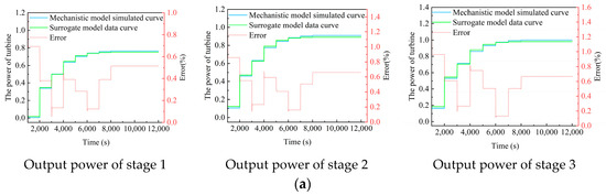
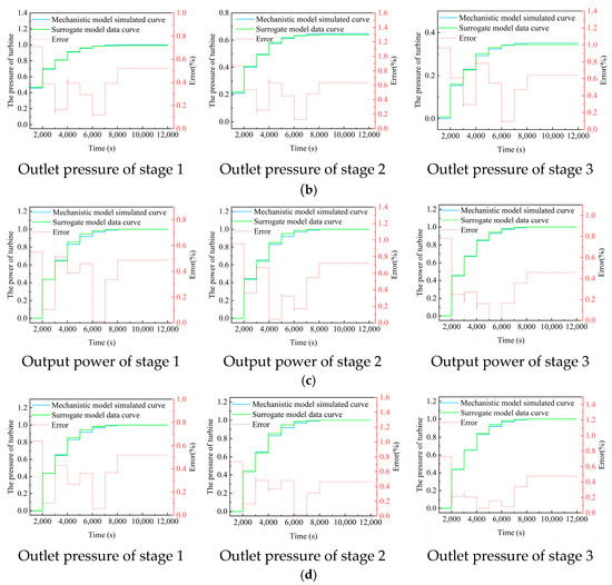
Figure 8.
Validation results of the steady-state surrogate model: (a) Comparison of output power results between the physics-based model and the surrogate model for stages 1–3 of the high-pressure section; (b) Comparison of outlet pressure results between the physics-based model and the surrogate model for stages 1–3 of the high-pressure section; (c) Comparison of output power results between the physics-based model and the surrogate model for stages 1–3 of the low-pressure section; (d) Comparison of outlet pressure results between the physics-based model and the surrogate model for stages 1–3 of the low-pressure section.
Under the same given boundary conditions, the obtained validation results are shown in Figure 8. As can be seen from the figure, under different operating conditions, the simulation results of the trained surrogate model are in good agreement with those of the physics-based model. The gap between the curves after normalization is due to the min–max normalization method. The actual absolute error between the two is within 1.57%, further validating the surrogate model’s rationality. The computational efficiency was quantitatively evaluated through comparative trials between the proposed SVR-based surrogate model and the traditional physical-based model simulations. The physics-based model required 18.7 ± 2.3 s per simulation due to equation iterations, while the surrogate model completed predictions in 2.8 ± 0.4 s through matrix operations. This demonstrates an 85.0% reduction in computational latency (Δt = (18.7 − 2.8)/18.7 × 100%), meeting real-time requirements for turbine control cycles.
As shown in Table 4, while meeting the real-time requirements, the turbine surrogate model demonstrates high accuracy for both the inlet pressure and power in the high-pressure and low-pressure sections. Whether analyzed based on average error or maximum error, the errors are maintained at a low level.
Table 4.
Comparison of surrogate model accuracy for the high-pressure and low-pressure sections.
4.2. Transient Response Compensation Effectiveness
To validate the model’s effectiveness under transient conditions, we selected an MST steam turbine operating condition step change as an example. Historical simulation data from the physical-based and steady-state surrogate models were used to train the error correction model. At t = 1000 s, after collecting sufficient historical data, the model began correcting the turbine’s power output predictions. The corrected results are shown in Figure 9.
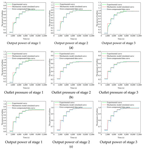
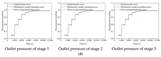
Figure 9.
Error compensation and correction results for the MST: (a) Error compensation results for output power of stages 1–3 in the high-pressure section; (b) Error compensation results for outlet pressure of stages 1–3 in the high-pressure section; (c) Error compensation results for output power of stages 1–3 in the low-pressure section; (d) Error compensation results for outlet pressure of stages 1–3 in the high-pressure section.
4.3. Comparative Analysis of Hybrid Model Performance
The steady-state model is developed based on physics-based simulation data and may still exhibit deviations from actual measurement data, as shown in Figure 8. Especially during dynamic transient responses, the error compensation model established using the Bi-LSTM time-series neural network algorithm effectively compensates for these errors. The data fusion model results show a higher fit with the actual data, reducing the error to the levels shown in Table 5. Compared to the results before error correction, the average maximum error in both the high-pressure and low-pressure sections is significantly reduced, and the overall average error in the system shows a clear decrease before and after the correction.
Table 5.
Comparison of errors before and after correction.
Traditional physics-based models suffer from slow computation due to multi-domain iterative coupling, while purely data-driven models [13,14] lack physical interpretability and fail under unseen conditions. Our hybrid approach uniquely combines physical constraints with data-driven efficiency: the SVR-based steady-state surrogate reduces computation time by 85% (from 18.7 s to 2.8 s per simulation) compared to full-order models, while the Bi-LSTM dynamic compensator improves transient prediction accuracy by 14.85% over standalone SVR models (see Table 3). This dual-layer architecture ensures both real-time capability and adherence to thermodynamic principles, overcoming the limitations of prior single paradigm methods.
5. Conclusions
This study proposes an innovative digital twin modeling approach for MSTs, resolving the critical trade-off between real-time computation and prediction accuracy through the synergistic integration of physics-based and data-driven models. Key conclusions are manifested in three aspects:
- A hierarchical modular architecture based on Modelica achieves cross-domain coupling of mechanical, thermodynamic, and hydrodynamic systems. By coordinating subsystem optimization with system-level fidelity design, it balances global accuracy with local modeling flexibility.
- An SVR model demonstrates a 1.57% absolute prediction error under step-load conditions while improving computational efficiency by 85% compared with conventional physics-based models, unifying precision and real-time performance.
- The proposed hybrid SVR-BiLSTM surrogate model integrates steady-state mapping with dynamic error compensation, reducing maximum absolute transient prediction error by 14.85% compared with standalone SVR implementations.
This framework provides a scalable template for intelligent upgrades of MST systems, with transferable multi-domain collaborative modeling methodology applicable to smart operation scenarios of other industrial equipment. Future research will expand digital twin applications in fault diagnosis and health management, and propel MST systems toward cognitive digital twin evolution.
Author Contributions
Conceptualization, Y.L. and D.S.; methodology, Y.L. and D.S.; validation, L.C. and X.L.; data curation, G.Y.; writing—original draft preparation, Y.L.; writing—review and editing, D.S.; visualization, D.S. and G.L.; supervision, L.C. and G.L. All authors have read and agreed to the published version of the manuscript.
Funding
This research received no external funding.
Data Availability Statement
No new data were created during this study. The data that support the findings are either publicly available or have been deposited in a public repository as outlined above.
Conflicts of Interest
Author Guihao Yin was employed by the company Suzhou Tongyuan Software & Control Technology Co., Ltd. The remaining authors declare that the research was conducted in the absence of any commercial or financial relationships that could be construed as a potential conflict of interest.
Abbreviations
The following abbreviations are used in this manuscript:
| Abbreviations | |
| O&M | Operations and maintenance |
| SVR | Support vector regression |
| SVM | Support vector machine |
| LSTM | Bidirectional long short-term memory |
| Bi-LSTM | Long short-term memory |
| RNN | Recurrent neural networks |
| RBF | Radial basis function |
| HP | High-pressure |
| LP | Low-pressure |
| Nomenclature | |
| Symbol | Paraphrase |
| Steam flow rates at the turbine inlet during the dynamic process (kg/s) | |
| Steam flow rates at the turbine inlet under the design condition (kg/s) | |
| Inlet pressures of the turbine during the dynamic process (MPa) | |
| Inlet pressures of the turbine under the design condition (MPa) | |
| Steam temperatures at the turbine inlet during the dynamic process (K) | |
| Steam temperatures at the turbine inlet under the design condition (K) | |
| Entropy values of the steam at the turbine inlet (kJ/K) | |
| Entropy values of the steam at the turbine outlet (kJ/K) | |
| Enthalpy value at the turbine inlet during isentropic expansion (kJ) | |
| Actual outlet enthalpy value of the steam (kJ) | |
| Enthalpy value at the turbine outlet during the isentropic expansion process (kJ) | |
| Outlet pressures of the turbine during the dynamic process (MPa) | |
| Actual shaft work output (kW) | |
| Moment of inertia (kg·m2) | |
| Output torque (kg·m) | |
| Output torque (kg·m) | |
| Angular velocity of the rotor (rad/s) | |
| Flow coefficient of the valve | |
| Flow coefficient of the valve at its maximum opening | |
| Density of the medium (kg·m3) | |
| Medium flow rates through the valve (kg/s) | |
| Maximum flow rates through the valve (kg/s) | |
| Pressure drop across the valve. | |
| W | The weight vectors |
| Input feature data at the current time step | |
| Memory cell state from the previous time step | |
| Hidden state (output information) from the previous time step | |
| b | The bias vectors |
| Element-wise multiplication | |
| Activation functions. | |
References
- Madusanka, N.S.; Fan, Y.; Yang, S.; Xiang, X. Digital Twin in the Maritime Domain: A Review and Emerging Trends. J. Mar. Sci. Eng. 2023, 11, 1021. [Google Scholar] [CrossRef]
- Inturi, V.; Ghosh, B.; Rajasekharan, S.G.; Pakrashi, V. A Review of Digital Twinning for Rotating Machinery. Sensors 2024, 24, 5002. [Google Scholar] [CrossRef]
- Orhan, M.; Celik, M. A Literature Review and Future Research Agenda on Fault Detection and Diagnosis Studies in Marine Machinery Systems. Proc. Inst. Mech. Eng. Part M J. Eng. Marit. Environ. 2024, 238, 3–21. [Google Scholar] [CrossRef]
- Lehtomäki, A. Digital Twin Model for a Gas Turbine. Master’s Thesis, LUT University, Lappeenranta, Finland, 2024. [Google Scholar]
- Grieves, M.; Vickers, J. Digital Twin: Mitigating Unpredictable, Undesirable Emergent Behavior in Complex Systems. In Transdisciplinary Perspectives on Complex Systems: New Findings and Approaches; Springer: Cham, Switzerland, 2017; pp. 85–113. [Google Scholar] [CrossRef]
- Chetan, M.; Yao, S.; Griffith, D.T. Multi-Fidelity Digital Twin Structural Model for a Sub-Scale Downwind Wind Turbine Rotor Blade. Wind Energy 2021, 24, 1368–1387. [Google Scholar] [CrossRef]
- Shangguan, D.; Chen, L.; Ding, J. A Digital Twin-Based Approach for the Fault Diagnosis and Health Monitoring of a Complex Satellite System. Symmetry 2020, 12, 1307. [Google Scholar] [CrossRef]
- Cameretti, C.M.; Robbio, D.R. Computational and Data-Driven Modelling of Combustion in Reciprocating Engines or Gas Turbines. Energies 2024, 17, 3863. [Google Scholar] [CrossRef]
- Macchi, M.; Roda, I.; Negri, E.; Fumagalli, L. Exploring the Role of Digital Twin for Asset Lifecycle Management. IFAC-Pap. 2018, 51, 790–795. [Google Scholar] [CrossRef]
- Kim, J.; Kim, S.-A. Lifespan Prediction Technique for Digital Twin-Based Noise Barrier Tunnels. Sustainability 2020, 12, 2940. [Google Scholar] [CrossRef]
- Hu, M.-Y.; Kong, F.-L.; Yu, D.-L.; Yang, J. Digital Twin’s Key Technologies and Application Prospects in the Field of Advanced Nuclear Energy. Power Syst. Technol. 2021, 45, 2514–2522. [Google Scholar] [CrossRef]
- Onaji, I.; Tiwari, D.; Soulatiantork, P.; Song, B.; Tiwari, A. Digital Twin in Manufacturing: Conceptual Framework and Case Studies. Int. J. Comput. Integr. Manuf. 2022, 35, 831–858. [Google Scholar] [CrossRef]
- Mrzljak, V.; Poljak, I.; Mrakovčić, T. Energy and Exergy Analysis of the Turbo-Generators and Steam Turbine for the Main Feed Water Pump Drive on LNG Carrier. Energy Convers. Manag. 2017, 140, 307–323. [Google Scholar] [CrossRef]
- Yu, J.; Liu, P.; Li, Z. Hybrid Modelling and Digital Twin Development of a Steam Turbine Control Stage for Online Performance Monitoring. Renew. Sustain. Energy Rev. 2020, 133, 110092. [Google Scholar] [CrossRef]
- Zhang, L.; Yang, Z.-C.; Liu, H.-R.; Chen, G.-B. Study on the Characteristics of Marine Nuclear Steam Turbine Units under Coupling off Design Conditions and Its Influencing Factors. Turbine Technol. 2019, 61, 266–270. [Google Scholar]
- Sun, T.; Liu, Y.; Ma, Z.; Shu, P.; Ye, Z. Numerical Simulation of the Relationship between Steam Flow Excitation Characteristics and Coverage on the Governing Stage of Marine Steam Turbine. Ocean Eng. 2024, 314, 119526. [Google Scholar] [CrossRef]
- Nirbito, W.; Budiyanto, M.A.; Muliadi, R. Performance Analysis of Combined Cycle with Air Breathing Derivative Gas Turbine, Heat Recovery Steam Generator, and Steam Turbine as LNG Tanker Main Engine Propulsion System. J. Mar. Sci. Eng. 2020, 8, 726. [Google Scholar] [CrossRef]
- Dulau, M.; Bica, D. Mathematical Modelling and Simulation of the Behavior of the Steam Turbine. Procedia Technol. 2014, 12, 723–729. [Google Scholar] [CrossRef]
- Mrzljak, V.; Jelić, M.; Poljak, I.; Prpić-Oršić, J. Analysis and Comparison of Main Steam Turbines from Four Different Thermal Power Plants. Pomorstvo 2023, 37, 58–74. [Google Scholar] [CrossRef]
- Poljak, I.; Mrzljak, V. Thermodynamic Analysis and Comparison of Two Marine Steam Propulsion Turbines. Naše More Znanstveni časopis Za More I Pomorstvo 2023, 70, 88–102. [Google Scholar]
- Sang, L.; Zhang, T. Fault Diagnosis of Steam Turbine Generator Unit Based on Support Vector Machine. In Proceedings of the 2013 2nd International Conference on Measurement, Information and Control, Harbin, China, 16–18 August 2013. [Google Scholar] [CrossRef]
- Loaiza, J.H.; Cloutier, R.J.; Lippert, K. Proposing a Small-Scale Digital Twin Implementation Framework for Manufacturing from a Systems Perspective. Systems 2023, 11, 41. [Google Scholar] [CrossRef]
- Ding, H.; Zhang, Y.; Ye, K.; Hong, G. Development of a Model for Thermal-Hydraulic Analysis of Helically Coiled Tube Once-through Steam Generator Based on Modelica. Ann. Nucl. Energy 2020, 137, 107069. [Google Scholar] [CrossRef]
- Suk Kim, J.; McKellar, M.; Bragg-Sitton, S.M.; Boardman, R.D. Status on the Component Models Developed in the Modelica Framework: High-Temperature Steam Electrolysis Plant & Gas Turbine Power Plant; Idaho National Lab. (INL): Idaho Falls, ID, USA, 2016. [Google Scholar] [CrossRef]
- Belli, K.G.; Esenboğa, B.; Yavuzdeğer, A.; Demirdelen, T. Design and Energy Efficiency Analysis of a Shaft Generator for Military Ships. Turk. J. Electr. Power Energy Syst. 2024, 4. [Google Scholar] [CrossRef]
- Yang, Y.; Wu, W.; Wu, J.; Zheng, Z. Simulation Analysis on Performance of Fast Variable Load for Marine Steam Power System. Chin. J. Ship Res. 2018, 13, 121–125. [Google Scholar]
- Zeng, G.; Wang, J.; Zhang, L.; Xie, X.; Wang, X.; Chen, G. Multi-Domain Modeling and Analysis of Marine Steam Power System Based on Digital Twin. J. Mar. Sci. Eng. 2023, 11, 429. [Google Scholar] [CrossRef]
- Zhang, P.; Xu, W. Steam Turbine Anomaly Detection: An Unsupervised Learning Using Enhanced LSTM Variational Autoencoder. Res. Sq. 2024. [Google Scholar] [CrossRef]
- Zhu, G.; Yang, L.; Liu, S.; Cheng, G. Boiler Water-Steam System Modeling and Calibration Based on Modelica. Model. Simul. 2014, 3, 25. [Google Scholar] [CrossRef]
- Cai, W.; Wen, X.; Li, C. Predicting the Energy Consumption in Buildings Using the Optimized Support Vector Regression Model. Energy 2023, 273, 127188. [Google Scholar] [CrossRef]
- Wang, J.; Liu, J.; Lu, Y. Machine Learning-Driven High-Fidelity Ensemble Surrogate Modelling of Francis Turbine Unit Based on Data-Model Interactive Simulation. Eng. Appl. Artif. Intell. 2024, 133, 108385. [Google Scholar] [CrossRef]
- Masood, Z.; Khan, S.; Qian, L. Machine Learning-Based Surrogate Model for Accelerating Simulation-Driven Optimisation of Hydropower Kaplan Turbine. Renew. Energy 2021, 173, 827–848. [Google Scholar] [CrossRef]
- Khan, M.R.; Shohanuzzaman, M.; Hosen, I.; Hassan, M.S. SVM-plus: An Improved Machine Learning Classifier to Predict Loss-of-Coolant Accidents in Pressurized Water Reactor. In Proceedings of the 2024 3rd International Conference on Advancement in Electrical and Electronic Engineering (ICAEEE), Gazipur, Bangladesh, 25–27 April 2024; IEEE: Piscataway, NJ, USA, 2024; pp. 1–6. [Google Scholar]
- Schirmann, M. Physics-Informed Data-Driven Models for Ship Response Prediction Using Global Wave Data. Ph.D. Thesis, University of Michigan, Ann Arbor, MI, USA, 2021. [Google Scholar]
- Watanabe, Y.; Takahashi, T.; Suzuki, K. Dynamic Simulation of an Oxygen-Hydrogen Combustion Turbine System Using Modelica. In Proceedings of the Modelica Conferences, Dallas, TX, USA, 26–28 October 2022; pp. 15–24. [Google Scholar]
- Asgari, S.; Moazamigoodarzi, H.; Tsai, P.J.; Pal, S.; Zheng, R.; Badawy, G.; Puri, I.K. Hybrid Surrogate Model for Online Temperature and Pressure Predictions in Data Centers. Future Gener. Comput. Syst. 2021, 114, 531–547. [Google Scholar] [CrossRef]
- Lim, J.Y.; Li, J.; O’Grady, D.; Downar, T.; Duraisamy, K. A Hybrid Surrogate Modeling Framework for the Digital Twin of a Fluoride-Salt-Cooled High-Temperature Reactor (FHR). Nucl. Eng. Des. 2025, 433, 113690. [Google Scholar] [CrossRef]
- Kozlovska, M.; Petkanic, S.; Vranay, F.; Vranay, D. Enhancing Energy Efficiency and Building Performance through BEMS-BIM Integration. Energies 2023, 16, 6327. [Google Scholar] [CrossRef]
- Talah, D.; Bentarzi, H.; Mangola, G. Modeling and Simulation of an Operating Gas Turbine Using Modelica Language. Rev. Roum. Sci. Tech.-Sér. Électrotech. Énerg. 2023, 68, 102–107. [Google Scholar]
- Guo, M.; Hao, Y.; Nižetić, S.; Lee, K.Y.; Sun, L. Modelica-Based Heating Surface Modelling and Dynamic Exergy Analysis of 300 MW Power Plant Boiler. Energy Convers. Manag. 2024, 312, 118557. [Google Scholar] [CrossRef]
- Rua Pazos, J. Dynamic Modeling and Process Simulation of Steam Bottoming Cycle. Master’s Thesis, NTNU, Trondheim, Norway, 2017. [Google Scholar]
- Reddy, A.S.; Ahmed, M.I.; Kumar, T.S.; Reddy, A.V.K.; Bharathi, V.P. Analysis of Steam Turbines. Int. Ref. J. Eng. Sci. 2014, 3, 32–48. [Google Scholar]
- Gülen, S.C. Gas and Steam Turbine Power Plants: Applications in Sustainable Power; Cambridge University Press: Cambridge, UK, 2023. [Google Scholar]
Disclaimer/Publisher’s Note: The statements, opinions and data contained in all publications are solely those of the individual author(s) and contributor(s) and not of MDPI and/or the editor(s). MDPI and/or the editor(s) disclaim responsibility for any injury to people or property resulting from any ideas, methods, instructions or products referred to in the content. |
© 2025 by the authors. Licensee MDPI, Basel, Switzerland. This article is an open access article distributed under the terms and conditions of the Creative Commons Attribution (CC BY) license (https://creativecommons.org/licenses/by/4.0/).