Abstract
Efficient ship scheduling in inland waterways is critical for maritime transportation safety and economic viability. However, traditional scheduling methods, primarily based on First Come First Served (FCFS) principles, often produce suboptimal results due to their inability to account for complex spatial–temporal dependencies, directional asymmetries, and varying ship characteristics. This paper introduces SSRL (Ship Scheduling through Reinforcement Learning), a novel framework that addresses these limitations by integrating three complementary components: (1) a Q-learning framework that discovers optimal scheduling policies through environmental interaction rather than predefined rules; (2) a clustering mechanism that reduces the high-dimensional state space by grouping similar ship states; and (3) a sliding window approach that decomposes the scheduling problem into manageable subproblems, enabling real-time decision-making. We evaluated SSRL through extensive experiments using both simulated scenarios and real-world data from the Xiaziliang Restricted Waterway in China. Results demonstrate that SSRL reduces total ship waiting time by 90.6% compared with TSRS, 48.4% compared with FAHP-ES, and 32.6% compared with OSS-SW, with an average reduction of 57.2% across these baseline methods. SSRL maintains superior performance across varying traffic densities and uncertainty conditions, with the optimal information window length of 13–14 ships providing the best balance between solution quality and computational efficiency. Beyond performance improvements, SSRL offers significant practical advantages: it requires minimal computation for online implementation, adapts to dynamic maritime environments without manual reconfiguration, and can potentially be extended to other complex transportation scheduling domains.
1. Introduction
1.1. Background
Maritime transportation stands as a cornerstone of global trade, recognized for its superior efficiency, environmental friendliness, and cost-effectiveness compared with other transportation modes [1,2]. Within the maritime sector, inland waterway transportation has emerged as a strategic priority, particularly in China, where it serves as a vital channel for domestic economic circulation and long-distance bulk cargo transport. According to the latest data from China’s Ministry of Transport, the nation’s waterway cargo volume surpassed 9.37 billion tons in 2023, with inland waterway shipping achieving a cargo volume of 4.79 billion tons and a cargo turnover of 2077.254 billion ton-kilometers [3]. Despite representing 8.6% of China’s total freight traffic with an estimated economic impact of 3.0 trillion RMB annually, this proportion remains below optimal levels for a comprehensive transportation system [3,4].
The growing shipping volume particularly impacts the middle and upper reaches of the Yangtze River, where geographical features create natural navigational challenges. In these regions, restricted waterways are defined as specialized one-way traffic systems with narrow, winding channels and torrential water flows, as illustrated in Figure 1. These waterways typically extend for 1 to 5 km and create bottlenecks that limit vessel visibility and maneuverability [5]. To address these challenges, China has established signal stations at each restricted waterway to optimize ship scheduling and minimize waiting times [6], which delivers significant economic benefits by reducing operational costs for shipping companies, environmental advantages through decreased emissions from idling vessels, and operational improvements via enhanced waterway throughput capacity and increased supply chain reliability [7,8].
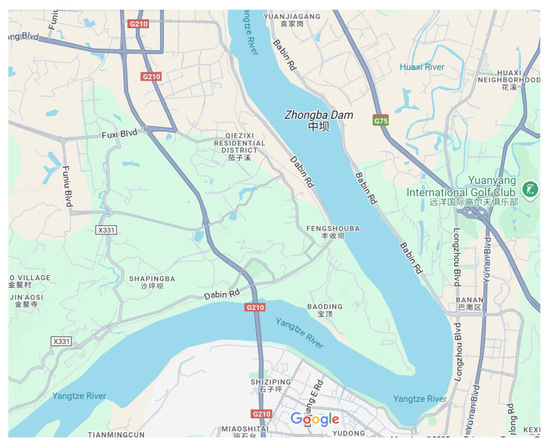
Figure 1.
Google map of Xiaziliang restricted waterway.
Two primary approaches exist to enhance the restricted waterway efficiency. The first approach is channelization, which involves physical infrastructure constructions to create straighter, deeper, and wider channels [9]. While this method can substantially improve waterway capacity, it requires significant capital investment, necessitates temporary waterway closures, and may introduce environmental disruptions [10,11]. The second approach, intelligent ship scheduling, focuses on optimizing ship passing sequences through advanced algorithms [12,13]. Although this method does not increase physical capacity [14], it offers a more cost-effective, environmentally friendly, and immediately deployable solution for improving navigational efficiency without disrupting existing operations [15].
1.2. Traditional Scheduling Methods in Restricted Waterways
Traditional scheduling methods in restricted waterways primarily rely on First Come First Served (FCFS) principles [16,17,18]. While FCFS approaches offer straightforward implementation and perceived fairness, they neglect critical operational factors, including varying vessel types, navigation speeds, and directional asymmetries [19,20]. These traditional rule-based methods represent non-machine learning approaches to ship scheduling, which rely on predetermined rules. FCFS inherently prioritizes temporal order over system-wide efficiency, leading to suboptimal utilization of waterway capacity, particularly during high traffic density periods [4,21]. Moreover, FCFS-based methods disregard the substantial time disparities between upstream and downstream navigation, which typically differ by a factor of 2–3 in restricted waterways throughout the Yangtze River system [5]. Such operational inefficiencies create a significant performance gap between current waterway management practices and China’s national strategic goal of developing a ‘strong transportation country’ with optimized inland waterway networks [22].
Several studies have investigated the effectiveness of FCFS-based scheduling. Jian et al. [23] developed a fluency model for restricted waterways using FCFS rules and evaluated its performance through Monte Carlo simulations, considering factors such as ship speed, arrival patterns, and waterway characteristics. Liu et al. [24] constructed a simulation model for the Three Gorges ship lock using the SIVAK platform, demonstrating that FCFS-based scheduling could reduce waiting times compared with sequential lock operations. To enhance FCFS performance, Lalla-Ruiz et al. [20] proposed a heuristic optimization algorithm that allows dynamic adjustment of ship sequences while maintaining the basic FCFS principle. Similarly, Gan et al. [17] extended the FCFS framework by incorporating safety constraints for restricted waterway operations.
While FCFS-based methods offer simplicity and fairness, they often lead to suboptimal solutions as they prioritize temporal equality over system efficiency. These methods fail to account for critical factors such as bi-directional traffic patterns, varying navigation times, and the substantial differences between upstream and downstream passage durations. Yang et al. [21] demonstrated that system-optimal scheduling for vessels passing through a waterway bottleneck could reduce costs significantly compared with non-coordinated FCFS approaches by accounting for both bunker costs and schedule delay penalties.
1.3. Intelligent Optimization Methods in Restricted Waterways
Recent advances in computational intelligence have enabled more sophisticated scheduling approaches to optimize ship sequences based on multiple objectives and constraints. Xin et al. [25] introduced a self-organizing model that first clusters ships based on arrival patterns and then optimizes intra-cluster scheduling to minimize ship-ship interference. Addressing congestion at the Three Gorges Dam, Zhao et al. [8] developed a hybrid meta-heuristic algorithm that simultaneously optimizes ship lift and lock scheduling. Xia et al. [7] proposed an integrated approach combining genetic algorithms with speed optimization to reduce both waiting time and carbon emissions. Liu et al. [4] introduced a fuzzy scheduling optimization method for one-way waterways that employs triangular fuzzy numbers to address uncertainty in vessel speeds and provides an algorithm for determining feasible tidal time windows. Their approach outperformed traditional rule-based methods while maintaining computational efficiency. In another study, Liu et al. [19] developed a ship scheduling model that addresses channel-lock coordination during flood season. Using a multi-population genetic algorithm, they demonstrated significant waiting time reduction in both normal and flood impact scenarios compared with independent scheduling approaches. Zhang et al. [11] proposed a model for ship scheduling in an anchorage-to-quay channel with water discharge restrictions. Their approach integrates ship sequencing at the anchorage, channel allocation, and berth planning while considering water discharge impacts to improve transportation efficiency and navigation safety.
Beyond the meta-heuristic and evolutionary approaches, researchers have further explored reinforcement learning frameworks for ship scheduling problems. Li et al. [26] proposed an adaptive heuristic algorithm based on reinforcement learning (GSAA-RL) for ship scheduling optimization, where Q-learning with a unique property of selecting suitable parameters dynamically is developed to adjust the parameters of crossover and mutation to improve the search ability of the algorithm. Their approach can significantly shorten the total time spent by ships in port compared with existing methods. Wang et al. [27] developed a hierarchical deep reinforcement learning framework for channel traffic scheduling in dry bulk export terminals, considering ship deballasting delays and dynamic switching traffic modes. Their approach is capable of producing integrated scheduling plans while minimizing ship mooring, unberthing, and deballasting delays, demonstrating superior performance compared with both traditional optimization methods and practical scheduling rules.
1.4. Research Gaps and Proposed Approach
Despite these advances, several critical challenges remain in the current literature. Unlike previous studies that allow the simultaneous passage of small ships in opposite directions, restricted waterways on the Yangtze River strictly prohibit bi-directional traffic due to safety concerns. Most existing methods assume variable ship speeds; however, speed adjustments are highly dangerous and practically infeasible in restricted waterways with torrential flows and sharp bends. Current approaches typically focus on arrival times while overlooking the significant variations in passage duration. Additionally, the dynamic nature of waterway traffic demands immediate scheduling decisions, yet most existing algorithms require substantial computational time.
Recent advances in artificial intelligence and machine learning present new opportunities for developing more sophisticated scheduling solutions that can adapt to dynamic maritime environments while maintaining computational efficiency. This paper introduces SSRL (Ship Scheduling through Reinforcement Learning), a novel algorithm that integrates three key components to overcome the technical challenges of ship scheduling in restricted waterways. First, unlike rule-based systems, SSRL employs Q-learning to discover efficient scheduling policies through environmental interaction, allowing the system to adapt to the complex dynamics of waterway traffic without relying on predefined rules. Second, to address the high-dimensional nature of the scheduling problem, SSRL utilizes a fuzzy clustering algorithm to group similar ship states, significantly reducing computational complexity while preserving essential traffic pattern information. Third, SSRL implements a novel sliding window approach that decomposes the scheduling problem into smaller, manageable subproblems by focusing on immediate-vicinity ships, enabling real-time decision-making in dynamic environments.
Our research makes several significant contributions to both the theoretical understanding and practical implementation of intelligent waterway management. We develop a comprehensive mathematical formulation of the restricted waterway scheduling problem that accounts for bi-directional traffic patterns, safety constraints, and varying navigation times. We demonstrate SSRL’s effectiveness through extensive simulation experiments, achieving an average 32% reduction in total waiting time compared with existing approaches, including the Traffic Signal Revealing System (TSRS), Online Ship Scheduling algorithm (OSS-SW), and Expert System-based algorithm (FAHP-ES). We also provide practical implementation guidelines, including optimal parameter settings for various traffic conditions, enabling straightforward adoption in real-world waterway management systems.
The remainder of this paper is structured as follows: Section 2 presents the mathematical formulation of the ship scheduling problem in restricted waterways. Section 3 details the proposed SSRL algorithm and its components. Section 4 describes the experimental validation and parameter optimization process. Finally, Section 5 concludes this paper with a summary of findings and future research directions.
2. The Ship Scheduling Problem in Restricted Waterways
The waterway traffic management department establishes a signaling system in each restricted waterway to regulate the ships’ passing sequence (as shown in Figure 2). Unlike on-road traffic light systems, the restricted waterway traffic management system delivers each ship either a ‘go’ signal or a ‘stop’ signal. Upon receiving a ‘go’ signal, a ship is authorized to enter the restricted waterway immediately. Conversely, upon receiving a ‘stop’ signal, the ship must wait outside the restricted waterway until it receives a ‘go’ signal.
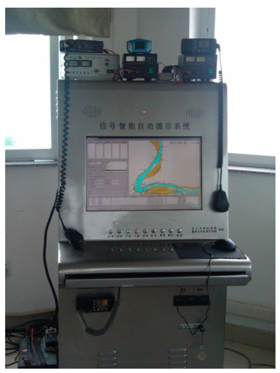
Figure 2.
Restricted waterway traffic management system.
Suppose N ships are scheduled to pass through a restricted waterway. The ith ship () arrives at the restricted waterway border at time and requires time to cross the waterway. The signal station must assign each ship an allowed entry time and an allowed crossing time . The denotes the permitted time for the ith ship to enter the restricted waterway, while represents the allocated duration for the ith ship to traverse the restricted waterway. Two metrics are widely adopted to quantify navigational efficiency: (1) total waiting time and (2) scheduled sequence length . The total waiting time represents the cumulative delay of all N ships and is defined by Equation (1):
The waiting time for the ith ship comprises two components: departure delay and traveling delay . The departure delay represents the time a ship waits for a ‘go’ signal outside the restricted waterway, while the traveling delay indicates additional time spent within the waterway to prevent overtaking. The scheduled sequence length quantifies the total time duration required for all N ships to pass through the restricted waterway and is defined by Equation (2):
In this equation, the first term identifies the time at which the last ship completes its passage through the restricted waterway, while the second term identifies the entry time of the first ship.
Both and are metrics for evaluating waterway scheduling efficiency. Although these metrics are not strictly equivalent, minimizing typically coincides with minimizing for the same set of ships. The metric focuses more on operational costs, while emphasizes waterway capacity. In this research, we adopt as the performance evaluation metric for the ship scheduling algorithm.
Table 1 demonstrates how optimized scheduling can reduce waiting time while maintaining safety constraints. The FCFS policy (scheduling sequence as 1→2→3→4) results in a total waiting time of 125 min. In contrast, the optimal sequence (2→3→1→4) prioritizes faster downstream ships, reducing the waiting time by 81.6% to 23 min. This example confirms the potential efficiency benefit when accounting for directional asymmetries in crossing times, particularly in bi-directional waterways where upstream and downstream navigation times differ substantially. Determining the optimal sequence becomes computationally intensive as the problem scales to include more ships, necessitating advanced optimized algorithmic approaches.

Table 1.
Comparison of FCFS-based ship scheduling policy and the optimal policy.
3. The Reinforcement Learning-Based Ship Scheduling Framework
3.1. Preliminaries
3.1.1. Reinforcement Learning
Reinforcement learning (RL) is one of the main domains of machine learning technology [28,29]. The key principle of RL is to develop a decision-making policy based on interactions and feedback from the environment, i.e., acting in an environment and updating the strategy according to the rewards received. This approach is particularly valuable for complex sequential decision problems like ship scheduling, where predetermined rules often fail to adapt to dynamic conditions.
Unlike supervised and unsupervised learning methods, RL learns to maximize the long-term reward of a Markov Decision Process (MDP) by experimenting with different actions and updating action values in response to environmental feedback, thus eliminating the need for predefined data [30]. For waterway management, this means shifting from fixed FCFS principles to adaptive scheduling policies that minimize collective waiting times. Generally, at time t, the agent observes the environmental state and takes an action according to policy , such that . The environment then transitions to a new state with probability and returns a reward to the agent. The agent aims to maximize total cumulative reward by selecting an appropriate sequence of actions. For an infinite-horizon MDP problem, the total discounted reward after time t is defined as:
where is the discount factor that balances the weight between immediate and future rewards. When approaches 1, the agent treats immediate and future rewards equally. Conversely, when approaches 0, the agent prioritizes immediate rewards and discounts future rewards. In the ship scheduling process, this allows balancing between optimizing for immediate traffic conditions and considering longer-term arrival patterns. The expected total reward given environmental state s under policy at time t is denoted by the state value function:
In addition to the state value function, the action value function (also known as Q-function) represents the expected reward starting from state s, taking action a, and following policy :
In practice, Q-learning is considered one of the most effective and efficient RL methods due to its integration of Monte Carlo and Dynamic Programming approaches [30,31]. The Q-learning constructs a Q-table to store values for all possible state–action combinations [32], which translates to evaluating different ship sequences under various traffic conditions for waterway management. The value of represents the expected reward of taking action a in state s. Given accurate Q-table values, the agent can identify the optimal action for each state by selecting the action with the highest Q-value. To determine these values, the Q-learning algorithm iteratively applies the Bellman Equation (6) to update Q-values for all state–action pairs until convergence:
where is the updated Q-value, combining the previous value with a new estimate . Here, represents the next state after taking action a in state s. The learning rate controls how much new information overrides existing information. A higher learning rate prioritizes new information; when , previous information is completely discarded, while ignores all new information. This iterative process enables the agent to accumulate knowledge about optimal actions across different states, making it ideal for discovering efficient ship scheduling policies that adapt to changing waterway conditions.
3.1.2. Clustering
Fuzzy C-Means (FCM) is a soft clustering algorithm that assigns membership degrees to each data point across all clusters based on distances between data points and cluster centers [33]. In ship scheduling applications, FCM is critical in discretizing continuous-time parameters, i.e., and . Given a dataset with N samples to be clustered into C groups, FCM aims to minimize the objective function in Equation (7) iteratively:
is a fuzziness index controlling the partition’s softness. Without prior domain knowledge, m is typically set to 2. The membership value indicates the probability of sample belonging to cluster j, such that
The term represents the center of the jth cluster, and denotes the similarity measure between data point and cluster center .
The objective function J is minimized when higher membership values are assigned to data points closer to cluster centers. Memberships and cluster centers are updated through the following equations:
The FCM algorithm is summarized in Algorithm 1. An appropriate number of clusters C is determined, followed by a random selection of initial cluster centers from the dataset. Centers and memberships are then updated iteratively until a stopping criterion is met, such as when membership changes become sufficiently small (Equation (11)) or when centers remain unchanged between consecutive iterations.
| Algorithm 1 FCM Clustering |
| Input: |
| Number of clusters C, Data set X, Fuzziness index m; |
| Output: |
| Cluster centers g, Membership matrix ; |
| 1: Randomly select C cluster centers; |
| 2: Calculate the initial memberships; |
| 3: repeat |
| 4: for to N do |
| 5: for to C do |
| 6: Update cluster centers according to Equation (10); |
| 7: end for |
| 8: end for |
| 9: for to N do |
| 10: for to C do |
| 11: Update membership values according to Equation (9); |
| 12: end for |
| 13: end for |
| 14: until stopping criterion is satisfied (Equation (11)) |
3.2. Proposed Scheduling Algorithm
This section describes our approach to establishing a real-time scheduling policy that guides ships through restricted waterways safely and efficiently. Specifically, we develop the scheduling policy using Q-learning while incorporating two key mechanisms to address the complex state and action spaces: (1) a DTW-based FCM clustering algorithm to identify similarities in ships’ states and group them into clusters, and (2) a sliding window mechanism to make the problem computationally tractable. Q-learning is selected as the core framework due to its model-free nature, which eliminates the need for explicit environment dynamics modeling, particularly advantageous for waterway scheduling where vessel interactions and environmental factors create complex dynamics. Additionally, Q-learning’s ability to balance exploration and exploitation is crucial for discovering optimal scheduling policies in the diverse traffic conditions of restricted waterways.
In standard Q-learning, a table stores Q-values for every possible state–action pair in the environment. However, in restricted waterway traffic management, ships’ predicted arrival times () and crossing times () are continuous variables, and the number of ships can be large. This results in a state space that is prohibitively large for conventional RL algorithms. The dimensionality challenge is addressed by the clustering mechanism through state abstraction, transforming high-dimensional continuous ship states into a manageable discrete set of representative clusters. This approach is valued for making the Q-learning problem computationally tractable and for enhancing generalization by allowing the algorithm to apply learned policies to novel but similar traffic patterns.
In our SSRL framework, the state space is composed of three key attributes for each ship: predicted arrival time (), crossing time (), and direction (d). For time t, the state of the ith ship is represented as , where represents the predicted arrival time of ship i at time t, represents its predicted crossing time, and indicates its direction (0 for downstream, 1 for upstream). The overall state is the collection of N ships’ states, , which are -dimensional data.
In our implementation, N is set to 30 based on practical considerations, resulting in a dimensional time series data. To reduce this high-dimensional state space, we employ FCM clustering to group similar environmental states into a manageable number of distinct clusters. Dynamic Time Warping (DTW) is adopted to calculate similarities between clusters because, unlike traditional distance metrics, DTW allows for ‘elastic’ transformations in time series data, making it particularly suitable for ship scheduling where temporal alignment is important. DTW can effectively capture the similarities in ship arrival and crossing time patterns regardless of local temporal variations.
After clustering, we identify C distinct clusters. States within the same cluster exhibit greater similarity than states in different clusters. This allows us to replace the high-dimensional ship state representation with a much smaller set of cluster identifiers, significantly reducing the Q-table size. The Q-learning process then proceeds as follows:
- Step 1: Initialize a Q-table with C rows (representing state clusters) and A columns (representing possible actions), where represents the expected reward for taking action a in state s.
- Step 2: Generate N ships with appropriate and values, calculate similarities with the C clusters, and assign the current state s to the cluster with the highest similarity.
- Step 3: Select a ship scheduling sequence a in state s using an -greedy policy: choose the action with the highest value with probability , or select a random action with probability .
- Step 4: Implement the selected sequence a by allocating appropriate and values to each ship to ensure safety. The environmental reward is computed based on the total waiting time (), incentivizing the agent to improve scheduling efficiency.
- Step 5: Update according to the Bellman Equation (6).
- Step 6: Repeat steps 3–5 until convergence criteria are met.
The detailed Q-learning process with FCM state reduction is formalized in Algorithm 2. The reward function is designed to minimize the total waiting time of ships. For each action (ship sequence) a taken in state s, the reward is defined as the negative sum of waiting times for all ships in that sequence:
where represents the departure delay (time spent waiting outside the waterway) and represents the traveling delay (additional time spent within the waterway). This reward structure incentivizes the Q-learning agent to prefer ship sequences that result in shorter overall waiting times while maintaining safety constraints. The negative formulation ensures compatibility with standard Q-learning algorithms that aim to maximize cumulative rewards. In our offline training process, this reward signal effectively guides the algorithm to discover scheduling policies that minimize total waiting times.
| Algorithm 2 Q-learning with FCM State Reduction |
| Input: |
| Number of clusters C, Number of actions A, Learning rate , |
| Discount factor , Exploration rate , Maximum episodes ; |
| Output: |
| Optimized Q-table; |
| 1: Initialize Q-table with dimensions with zeros; |
| 2: for to do |
| 3: Generate N ships with appropriate and values; |
| 4: Calculate similarity with the C clusters; |
| 5: Assign current state s to the cluster with highest similarity; |
| 6: // Select action using -greedy policy |
| 7: if then |
| 8: Select random action a; |
| 9: else |
| 10: Select action a with highest ; |
| 11: end if |
| 12: // Implement selected sequence |
| 13: Allocate appropriate and values to each ship; |
| 14: Ensure safety constraints are satisfied; |
| 15: // Calculate reward based on total waiting time |
| 16: ; |
| 17: // Observe new state |
| 18: Calculate similarity with the C clusters; |
| 19: Assign new state to the cluster with highest similarity; |
| 20: // Update Q-table using Bellman equation |
| 21: ; |
| 22: // Move to next state |
| 23: ; |
| 24: // Reduce exploration over time |
| 25: ; |
| 26: end for |
| 27: return Q-table; |
For a scheduling problem with N ships, the action space consists of possible ship sequences, which creates a combinatorial explosion as N increases. To address this challenge, SSRL employs a sliding window mechanism that divides the overall scheduling problem into manageable subproblems [34]. This mechanism utilizes two key parameters: (1) information window length (), which controls the number of ships considered in each subproblem, and (2) schedule window length (), which defines the number of ships actually scheduled in each iteration.
At each decision point, the first ships’ states are considered for sequencing, but only decisions for the first ships are implemented; the remaining ships are returned to the schedule list for subsequent iterations. This approach reduces the action space from to possibilities, making the problem computationally tractable while maintaining solution quality. Additionally, SSRL utilizes an -greedy exploration strategy during learning, selecting a random action with probability and the currently known best action with probability , with decreasing as learning progresses to shift from exploration to exploitation.
The sliding window approach is particularly suitable for dynamic waterway environments where future arrival information may be incomplete, allowing decisions based on the most current and reliable data while enhancing the agent’s ability to handle uncertainties by focusing each subproblem on ships with more reliable information. Since ships located far from the restricted waterway rarely navigate ahead of closer vessels, these mechanisms effectively transform the global optimization problem into tractable subproblems with sufficient action space exploration without exhaustive search.
Once the ship sequence is determined, each ship must be assigned an appropriate entry time () and crossing time () to ensure safe passage. The scheduling adheres to two fundamental principles: (1) overtaking is prohibited within restricted waterways, and (2) a minimum safety gap must be maintained between consecutive ships. Equations (13) and (14) formalize these constraints for ships traveling in the same and different directions, respectively, where represents the minimum required safety gap (typically set to 1 min in practice). These equations enforce safety through hard constraints rather than penalty terms in the reward function, ensuring a minimum safety gap between ships while prohibiting both overtaking and simultaneous entry of ships from opposite directions. By applying these constraints during action implementation, unsafe actions are excluded from the feasible space, prioritizing safety as non-negotiable while allowing the reward function to focus solely on efficiency optimization by incentivizing the agent to discover scheduling policies that minimize operational delays.
3.3. Computational Complexity and Performance Analysis
Benefiting from the ‘offline training, online application’ paradigm, SSRL resolves the traditional trade-off between accuracy and computational speed. While comprehensive Q-learning is computationally intensive, this process occurs offline, allowing sufficient time to build accurate decision policies. During practical operation, scheduling decisions involve only table lookup operations with complexity, guaranteeing instantaneous response regardless of traffic complexity.
SSRL demonstrates excellent scalability as the number of ships increases through three key mechanisms: (1) State abstraction: FCM clustering simplifies the high-dimensional state space into a fixed number of representative clusters. This ensures that even when the number of ships increases from N to , the number of clusters C remains constant, keeping the Q-table size independent of the total ship count. (2) Sliding window: The algorithm considers only ships in the information window, maintaining computational complexity at the level regardless of the total number of ships. This localized decision process allows SSRL to handle theoretically unlimited numbers of ships. This approach is particularly effective in restricted waterways where ships located far from the waterway rarely navigate ahead of closer vessels due to operational constraints. Our experimental design with 30 ships arriving within 1-h already represents an extremely congested scenario, as restricted waterways typically accommodate only 5–10 ships per hour due to their single-direction passage requirement. (3) Offline learning: The Q-learning process is completed offline using simulated data covering various traffic patterns. Once trained, the online deployment computational requirements remain at for table lookup operations, independent of the total number of ships.
In addition to computational efficiency, SSRL achieves an effective balance between scheduling accuracy and ship speed considerations through several mechanisms: (1) Reward function design: By using the negative sum of waiting times as the reward signal, SSRL naturally prioritizes faster ships (typically those traveling downstream with shorter crossing times) while maintaining overall scheduling accuracy. (2) State representation: The state space captures essential information about each ship’s arrival time (), crossing time (), and direction (d), providing the algorithm with comprehensive knowledge to balance the advantages of faster ships against overall traffic flow optimization. (3) Sliding window optimization: Our parameter analysis determined that and provide the optimal balance point where the algorithm has adequate foresight without excessive computational overhead or delayed response to faster vessels. (4) Efficient action space search: Despite the large theoretical action space of , our experimental results demonstrate that SSRL can effectively discover near-optimal ship sequences. This is achieved through the combination of -greedy exploration, strategic dimensionality reduction, and the inherent guidance provided by the reward signal toward more efficient scheduling arrangements.
These design features collectively enable SSRL to deliver highly optimized scheduling solutions that strategically sequence ships based on their directional speed characteristics while maintaining scheduling accuracy through comprehensive state representation and reward mechanisms. Experimental results confirm this balance achievement in congested scenarios where the tension between prioritizing faster ships and maintaining overall efficiency is highest.
4. Experiments and Results Analysis
Simulations and experiments were conducted to evaluate the effectiveness, efficiency, and robustness of the proposed algorithm. All tests were performed on a platform with an Intel i7 processor and 16GB of RAM, with no additional software installed to prevent interference.
4.1. Data Description
To simulate real-world scenarios of ships passing through restricted waterways, 30 ships arriving randomly at the restricted waterway border within periods of 1 to 3 h were considered. These scenarios cover a comprehensive range of traffic volumes, from highly congested (1 h) to moderate (2 h) and sparse (3 h) scenarios, ensuring our results are representative across all realistic operational conditions. The crossing time was sampled from Gaussian distributions , where and vary depending on ship direction and waterway characteristics. Based on analysis of AIS data collected from the Xiaziliang Restricted Waterway in China (shown in Figure 1), and were set to 18, 3 min and 49, 5 min for downstream and upstream travel, respectively.
4.2. Experimental Results and Parameter Sensitivity
Table 2 details scheduling results for 30 ships arriving at the restricted waterway within one hour under ideal conditions (no uncertainties). The table presents the original ship information and the resulting ship sequences determined by three benchmark methods—TSRS [5], FAHP-ES [5], and OSS-SW [17]—alongside our proposed SSRL algorithm. These established methods were chosen as benchmarks because they specifically address the unique operational constraints of restricted waterways in the Yangtze River system. For the SSRL algorithm, we set and , meaning the algorithm considered the first 10 ships’ information while applying scheduling decisions only to the first 5 ships in each step. The results indicate that our SSRL algorithm generated the optimal ship sequence that significantly reduced total waiting times. To ensure statistical validity, we conducted 100 independent experiments under identical conditions (30 ships arriving in one hour with no uncertainties), with results shown in Figure 3. The proposed SSRL algorithm consistently achieved the lowest total waiting time with the smallest variance, demonstrating both superior performance and stability compared with conventional approaches.
Table 2.
Scheduling results of 30 ships by different algorithms.
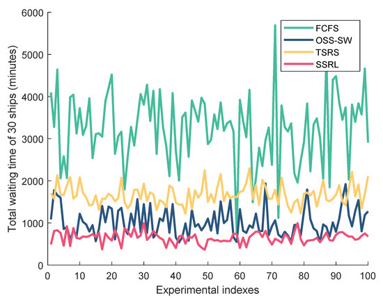
Figure 3.
Total waiting time of ships across 100 independent tests.
To comprehensively evaluate the SSRL algorithm’s performance, we designed 12 test cases with varying degrees of uncertainty and congestion (shown in Table 3). represents the percentage of ships appearing unexpectedly near the waterway border, while indicates the proportion of ships that dock before entering the waterway. To test the algorithm’s ability to handle these uncertainties, we implemented a 10 min notification time constraint. Ships appearing unexpectedly were added to the scheduling list only 10 min before their arrival at the waterway border, while docked ships were removed from the scheduling list 10 min before they stopped. For each case, we conducted 100 independent Monte Carlo simulations with varying from 10 to 30 and from 5 to 15.
Table 3.
Test cases with different parameter settings to evaluate the proposed algorithm.
Figure 4 illustrates the total waiting time of 30 ships scheduled by the SSRL algorithm as a function of schedule window length () and information window length (), which varied from 5 to 10 and 10 to 30, respectively. Each data point represents the mean value from 100 independent simulations. Figure 4a shows the least congested scenario with 30 ships arriving over 180 min, Figure 4b depicts the moderately congested scenario with ships arriving within 120 min, and Figure 4c presents the most congested scenario with all ships arriving within 60 min. The color gradient from blue to red represents increasing waiting times.
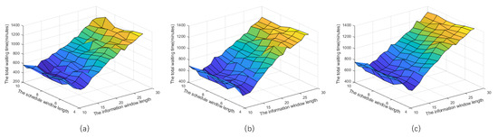
Figure 4.
Total waiting time for 30 ships under zero uncertainty scenarios, with ships arriving within: (a) 180 min; (b) 120 min; (c) 60 min.
As expected, waiting times increased with waterway congestion. In the most congested scenario (Figure 4c), the minimum waiting time was 670 min, compared with 313 and 503 min in Figure 4a and Figure 4b, respectively. The information window length () demonstrated a greater influence on algorithm performance than the schedule window length (). As increased, the total waiting time initially decreased before rapidly increasing in all scenarios. Minimum waiting times were consistently achieved when was approximately 13–14 and was 8.
We conducted additional experiments with varying degrees of uncertainty (sudden ship appearances and dockings) to comprehensively evaluate the SSRL algorithm’s robustness. Figure 5 presents these results, where the horizontal axis indicates the ship arrival time window (: 60, 120, or 180 min) and the vertical axis shows the mean waiting time across 100 simulations. The best performance was observed under conditions with no sudden ship appearances but with 10% of ships docking ( and ). Conversely, the highest waiting times occurred when 10% of ships appeared unexpectedly with no dockings ( and ). The two intermediate uncertainty scenarios yielded similar performance levels.
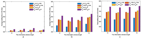
Figure 5.
Total waiting time for ships under 12 different test cases, with ships arriving within: (a) 180 min; (b) 120 min; (c) 60 min.
Beyond sliding window parameters, we conducted additional sensitivity analyses on core reinforcement learning parameters. For the learning rate (), our experiments with values ranging from 0.1 to 0.9 revealed that provides the best balance between learning speed and stability. Lower values resulted in slow convergence, while higher values occasionally produced significant oscillations in Q-values. We further enhanced stability by implementing an adaptive learning rate mechanism following , where is the initial learning rate, is a decay factor, and t is the episode number.
The discount factor () determines how the algorithm balances immediate versus future rewards. Values between 0.8 and 0.95 yielded similar performance, with being optimal in most scenarios. This indicates that both short-term efficiency and long-term strategic planning are important for effective waterway management.
For exploration-exploitation balancing, we compared several approaches, including Boltzmann exploration and fixed values. A decaying -greedy strategy starting with and diminishing at a rate of 0.995 per episode consistently delivered superior performance. This approach ensures thorough exploration of the complex action space during early training while gradually transitioning to exploitation of learned knowledge.
For the clustering algorithm, we found that 70 clusters provide the optimal balance between state space reduction and information preservation. These parameter optimization findings demonstrate that SSRL performance remains robust across reasonable parameter ranges, making the algorithm suitable for real-world deployment. Our analysis establishes a systematic methodology for parameter optimization that can be applied to other waterway scenarios beyond those tested in this study.
Computational efficiency is another critical factor for real-world applications, as ships must receive signals immediately upon arrival at the waterway border to prevent traffic chaos. The SSRL’s ‘offline training, online application’ paradigm determines optimal ship sequences by simply retrieving the maximum value from a precomputed knowledge table, requiring minimal computation for online scheduling.
4.3. Discussion
Based on the Monte Carlo simulations, the following conclusions regarding the SSRL algorithm’s performance for ship scheduling in restricted waterways are obtained:
(1) The proposed SSRL method consistently outperforms traditional approaches, including FCFS, OSS-SW, and TSRS. This superior performance stems from the Q-learning approach, which constructs a comprehensive lookup table storing values for all possible scheduling sequences under each state. These Q-values, representing the utility of each ship sequence in a given state, theoretically converge to optimal values with probability 1 as all possible sequences are repeatedly sampled across all states.
(2) The optimal information window length () for Xiaziliang restricted waterway traffic management is 13 ships. As shown in Figure 4, significantly impacts the SSRL algorithm’s performance. When varies between 10 and 30, the total waiting time follows a ‘V’ shape, with minimum waiting times occurring when is approximately 13. This pattern emerges because as increases, the number of possible ship sequences grows exponentially, making it difficult for the Q-learning algorithm to converge to optimal values. Conversely, if is too small, the search space becomes overly constrained, potentially excluding optimal sequences.
(3) The SSRL algorithm effectively manages restricted waterway uncertainties. Although Figure 5 shows significant variations in waiting times under different uncertainty conditions, this does not indicate a deficiency in handling uncertainties. These variations reflect differences in the number of ships ultimately scheduled: in cases 4–6, three ships dock () and are removed from the scheduling list, leaving only 27 ships; in cases 7–9, three additional ships appear unexpectedly (), resulting in 33 ships; in the remaining cases, exactly 30 ships are scheduled. The average waiting time per ship remains approximately 16 min across all scenarios, demonstrating the algorithm’s consistent performance regardless of uncertainty type.
(4) Total waiting time increases with traffic density. Figure 5c represents the most congested scenario, with 30 ships arriving within 60 min, resulting in the highest waiting time (approximately 35,000 min) across all cases. In contrast, Figure 5a shows the least congested scenario, with 30 ships distributed over 180 min, yielding the lowest waiting time (approximately 25,000 min). This pattern reflects the inherent capacity limitations of restricted waterways, where increased traffic density inevitably leads to greater congestion and correspondingly longer waiting times.
(5) The SSRL algorithm meets the real-time requirements essential for practical ship scheduling applications. Three key characteristics contribute to its computational efficiency: First, the algorithm performs all intensive learning processes offline, with online implementation requiring only simple table lookups. Second, state space dimensionality is substantially reduced through clustering ship information into a manageable number of groups. Finally, the sliding window mechanism further reduces both state and action space dimensions, enhancing computational efficiency.
5. Conclusions
Inefficient ship scheduling represents a significant bottleneck in restricted waterway traffic management. This paper introduces SSRL, a novel ship scheduling algorithm that integrates reinforcement learning with clustering and sliding window mechanisms. Unlike traditional scheduling approaches, SSRL learns optimal scheduling policies offline by evaluating all possible ship sequences and updating knowledge based on performance feedback. This allows online scheduling decisions to be made through efficient table lookups, minimizing computational requirements during operation.
We validated the SSRL algorithm through extensive experimentation comprising 12 cases, with 100 independent experiments conducted for each case. SSRL consistently demonstrated its superiority over conventional approaches in all scenarios, reducing waiting times by 90.6% compared with TSRS, 48.4% compared with FAHP-ES, and 32.6% compared with OSS-SW. Our comprehensive Monte Carlo simulations across various scenarios and parameter configurations further confirmed the algorithm’s effectiveness in managing ship scheduling under different uncertainty conditions. Parameter sensitivity analysis established that an information window length () of 13 ships combined with a schedule window length () of 8 ships provides the optimal balance between solution quality and computational efficiency in Xiaziliang Restricted Waterway. For reinforcement learning parameters, our analysis determined that a learning rate of (enhanced with adaptive decay where k = 0.001), discount factor , and a decaying -greedy strategy starting with and diminishing at a rate of 0.995 per episode consistently delivers superior performance across various traffic conditions. As expected, more congested waterways resulted in longer waiting times, reflecting physical capacity constraints.
The clustering algorithm and sliding window mechanism introduced in this work effectively address the dimensional challenges of the scheduling problem by reducing state space complexity. Future research could extend this approach by incorporating deep reinforcement learning techniques to handle even larger state spaces, potentially yielding more refined scheduling policies. Additional areas for investigation include adapting the algorithm for multi-waterway coordination and integrating real-time environmental factors such as weather conditions and visibility constraints.
While SSRL was validated using data from the Xiaziliang Restricted Waterway, its application to other restricted waterways with different characteristics requires parameter recalibration. Specifically, the Gaussian distribution parameters for upstream and downstream ships’ crossing times ( and ) vary based on waterway length, current velocity, and geometric features. However, the fundamental SSRL framework remains applicable across all restricted waterways with similar operational constraints of one-way traffic systems. This research contributes to the field of inland waterway transportation by providing a practical, efficient, and adaptable solution for real-time ship scheduling in restricted waterways, with potential applications extending to other complex transportation scheduling problems.
Author Contributions
Conceptualization, S.G. and H.L.; methodology, S.G. and X.W.; software, X.W.; validation, S.G., X.W. and H.L.; formal analysis, X.W.; investigation, S.G.; resources, H.L.; data curation, X.W.; writing—original draft preparation, S.G.; writing—review and editing, X.W. and H.L.; visualization, X.W.; supervision, H.L.; project administration, H.L.; funding acquisition, H.L. All authors have read and agreed to the published version of the manuscript.
Funding
This research was funded by the National Science Foundation of China (Grant No. 62003011) and Open Research Project of Big Data Application Technologies Laboratory, China Academy of Transportation Sciences (Grant No. 2021B1203).
Data Availability Statement
Restrictions apply to the availability of these data. Data was obtained from Changjiang Waterway Bureau and are available with the permission of Changjiang Waterway Bureau.
Conflicts of Interest
Author Hongdun Li is employed by the company China Academy of Transportation Sciences. The authors declare that this study received funding from the National Science Foundation of China and Open Research Project of China Academy of Transportation Sciences. The funder was not involved in the study design, collection, analysis, interpretation of data, the writing of this article, or the decision to submit it for publication.
References
- Buchem, M.; Golak, J.A.P.; Grigoriev, A. Vessel velocity decisions in inland waterway transportation under uncertainty. Eur. J. Oper. Res. 2022, 296, 669–678. [Google Scholar] [CrossRef]
- Zhang, J.; Wan, C.; He, A.; Zhang, D.; Soares, C.G. A two-stage black-spot identification model for inland waterway transportation. Reliab. Eng. Syst. Saf. 2021, 213, 107677. [Google Scholar] [CrossRef]
- Yang, W.; Liao, P.; Jiang, S.; Wang, H. Analysis of vessel traffic flow characteristics in inland restricted waterways using multi-source data. arXiv 2024, arXiv:2410.07130. [Google Scholar] [CrossRef]
- Liu, D.; Shi, G.; Kang, Z. Fuzzy scheduling problem of vessels in one-way waterway. J. Mar. Sci. Eng. 2021, 9, 1064. [Google Scholar] [CrossRef]
- Liang, S.; Yang, X.; Bi, F.; Ye, C. Vessel traffic scheduling method for the controlled waterways in the upper Yangtze River. Ocean Eng. 2019, 172, 96–104. [Google Scholar] [CrossRef]
- Gan, S.; Liang, S.; Li, K.; Deng, J.; Cheng, T. Ship trajectory prediction for intelligent traffic management using clustering and ANN. In Proceedings of the 2016 UKACC 11th International Conference on Control (CONTROL), Belfast, UK, 31 August–2 September 2016; pp. 1–6. [Google Scholar]
- Xia, Z.; Guo, Z.; Wang, W.; Jiang, Y. Joint optimization of ship scheduling and speed reduction: A new strategy considering high transport efficiency and low carbon of ships in port. Ocean Eng. 2021, 233, 109224. [Google Scholar] [CrossRef]
- Zhao, X.; Lin, Q.; Yu, H. A Co-Scheduling Problem of Ship Lift and Ship Lock at the Three Gorges Dam. IEEE Access 2020, 8, 132893–132910. [Google Scholar] [CrossRef]
- Fryirs, K.A.; Brierley, G.J.; Hancock, F.; Cohen, T.J.; Brooks, A.P.; Reinfelds, I.; Cook, N.; Raine, A. Tracking geomorphic recovery in process-based river management. Land Degrad. Dev. 2018, 29, 3221–3244. [Google Scholar] [CrossRef]
- Lagos, M.S.; Muñoz, J.F.; Suárez, F.I.; Fuenzalida, M.J.; Yáñez-Morroni, G.; Sanzana, P. Investigating the effects of channelization in the Silala River: A review of the implementation of a coupled MIKE-11 and MIKE-SHE modeling system. Wiley Interdiscip. Rev. Water 2024, 11, e1673. [Google Scholar] [CrossRef]
- Zhang, Y.; Liu, S.; Zheng, Q.; Tian, H.; Guo, W. Ship scheduling problem in an anchorage-to-quay channel with water discharge restrictions. Ocean Eng. 2024, 309, 118432. [Google Scholar] [CrossRef]
- Zhai, D.; Fu, X.; Xu, H.Y.; Yin, X.F.; Vasundhara, J.; Zhang, W. Multi-Layer Scheduling Optimization for Intelligent Mobility of Maritime Operation. In Proceedings of the 2020 15th IEEE Conference on Industrial Electronics and Applications (ICIEA), Kristiansand, Norway, 9–13 November 2020; pp. 1511–1514. [Google Scholar]
- Chen, C.; Chen, X. Scheduling optimization in restricted channels based on the agent technology and bayesian network. In Proceedings of the 2017 4th International Conference on Transportation Information and Safety (ICTIS), Banff, AB, Canada, 8–10 August 2017; pp. 291–295. [Google Scholar]
- Le Carrer, N.; Ferson, S.; Green, P.L. Optimising cargo loading and ship scheduling in tidal areas. Eur. J. Oper. Res. 2020, 280, 1082–1094. [Google Scholar] [CrossRef]
- Zhang, X.; Li, R.; Wang, C.; Xue, B.; Guo, W. Robust optimization for a class of ship traffic scheduling problem with uncertain arrival and departure times. Eng. Appl. Artif. Intell. 2024, 133, 108257. [Google Scholar] [CrossRef]
- Eisen, H.E.; Van der Lei, J.E.; Zuidema, J.; Koch, T.; Dugundji, E.R. An Evaluation of First-Come, First-Served Scheduling in a Geometrically-Constrained Wet Bulk Terminal. Front. Future Transp. 2021, 2, 709822. [Google Scholar] [CrossRef]
- Gan, S.; Wang, Y.; Li, K.; Liang, S. Efficient online one-way traffic scheduling for restricted waterways. Ocean Eng. 2021, 237, 109515. [Google Scholar] [CrossRef]
- Gan, S.; Liang, S.; Li, K.; Deng, J.; Cheng, T. Long-term ship speed prediction for intelligent traffic signaling. IEEE Trans. Intell. Transp. Syst. 2016, 18, 82–91. [Google Scholar] [CrossRef]
- Liu, S.; Zhang, Y.; Guo, W.; Tian, H.; Tang, K. Ship scheduling problem based on channel-lock coordination in flood season. Expert Syst. Appl. 2024, 254, 124393. [Google Scholar] [CrossRef]
- Lalla-Ruiz, E.; Shi, X.; Voß, S. The waterway ship scheduling problem. Transp. Res. Part D Transp. Environ. 2018, 60, 191–209. [Google Scholar] [CrossRef]
- Yang, X.; Gu, W.; Wang, S. Optimal scheduling of vessels passing a waterway bottleneck. Ocean Coast. Manag. 2023, 244, 106809. [Google Scholar] [CrossRef]
- Aritua, B.; Cheng, L.; van Liere, R.; de Leijer, H. Blue Routes for a New Era: Developing Inland Waterways Transportation in China; World Bank Publications: Herndon, VA, USA, 2021. [Google Scholar]
- Jian, L.; Xing, Y.; Ke-zhong, L.; Zhi-tao, Y. Study on the fluency of one-way waterway transportation based on First Come First Served (FCFS) model. In Proceedings of the 2015 International Conference on Transportation Information and Safety (ICTIS), Wuhan, China, 25–28 June 2015; pp. 669–674. [Google Scholar]
- Liu, Y.; Mou, J.M. Simulation on the traffic capacity of the Three Gorges ship lock based on SIVAK. J. Dalian Marit. Univ. 2015, 41, 37–41. [Google Scholar]
- Xin, X.; Liu, K.; Zhang, J.; Chen, S.; Wang, H.; Cheng, Z. A Self-Organizing Grouping Approach for Ship Traffic Scheduling in Restricted One-Way Waterway. Mar. Technol. Soc. J. 2019, 53, 83–96. [Google Scholar] [CrossRef]
- Li, R.; Zhang, X.; Jiang, L.; Yang, Z.; Guo, W. An adaptive heuristic algorithm based on reinforcement learning for ship scheduling optimization problem. Ocean Coast. Manag. 2022, 230, 106375. [Google Scholar] [CrossRef]
- Wang, W.; Ding, A.; Cao, Z.; Peng, Y.; Liu, H.; Xu, X. Deep Reinforcement Learning for Channel Traffic Scheduling in Dry Bulk Export Terminals. IEEE Trans. Intell. Transp. Syst. 2024, 25, 17547–17561. [Google Scholar] [CrossRef]
- Kiran, B.R.; Sobh, I.; Talpaert, V.; Mannion, P.; Al Sallab, A.A.; Yogamani, S.; Pérez, P. Deep reinforcement learning for autonomous driving: A survey. IEEE Trans. Intell. Transp. Syst. 2021, 23, 4909–4926. [Google Scholar] [CrossRef]
- Haydari, A.; Yilmaz, Y. Deep reinforcement learning for intelligent transportation systems: A survey. IEEE Trans. Intell. Transp. Syst. 2020, 23, 11–32. [Google Scholar] [CrossRef]
- Fan, J.; Wang, Z.; Xie, Y.; Yang, Z. A theoretical analysis of deep Q-learning. In Proceedings of the Learning for Dynamics and Control, PMLR, Virtual, 13–18 July 2020; pp. 486–489. [Google Scholar]
- Tong, Z.; Chen, H.; Deng, X.; Li, K.; Li, K. A scheduling scheme in the cloud computing environment using deep Q-learning. Inf. Sci. 2020, 512, 1170–1191. [Google Scholar] [CrossRef]
- Zhang, Q.; Lin, M.; Yang, L.T.; Chen, Z.; Khan, S.U.; Li, P. A double deep Q-learning model for energy-efficient edge scheduling. IEEE Trans. Serv. Comput. 2018, 12, 739–749. [Google Scholar] [CrossRef]
- Lei, T.; Jia, X.; Zhang, Y.; He, L.; Meng, H.; Nandi, A.K. Significantly fast and robust fuzzy c-means clustering algorithm based on morphological reconstruction and membership filtering. IEEE Trans. Fuzzy Syst. 2018, 26, 3027–3041. [Google Scholar] [CrossRef]
- Mattingley, J.; Wang, Y.; Boyd, S. Receding horizon control. IEEE Control Syst. 2011, 31, 52–65. [Google Scholar]
Disclaimer/Publisher’s Note: The statements, opinions and data contained in all publications are solely those of the individual author(s) and contributor(s) and not of MDPI and/or the editor(s). MDPI and/or the editor(s) disclaim responsibility for any injury to people or property resulting from any ideas, methods, instructions or products referred to in the content. |
© 2025 by the authors. Licensee MDPI, Basel, Switzerland. This article is an open access article distributed under the terms and conditions of the Creative Commons Attribution (CC BY) license (https://creativecommons.org/licenses/by/4.0/).