Dual-Channel Spoofed Speech Detection Based on Graph Attention Networks

Abstract

In the field of voice cryptography, detecting forged speech is crucial for secure communication and identity authentication. While most existing spoof detection methods rely on monaural audio, the characteristics of dual-channel signals remain underexplored. To address this, we propose a symmetrical dual-branch detection framework that integrates Res2Net with coordinate attention (Res2NetCA) and a dual-channel heterogeneous graph fusion module (DHGFM). The proposed architecture encodes left and right vocal tract signals into spectrogram and time-domain graphs, and it models both intra- and inter-channel time–frequency dependencies through graph attention mechanisms and fusion strategies. Experimental results on the ASVspoof2019 and ASVspoof2021 LA datasets demonstrate the superior detection performance of our method. Specifically, it achieved an EER of 1.64% and a Min-tDCF of 0.051 on ASVspoof2019, and an EER of 6.76% with a Min-tDCF of 0.3638 on ASVspoof2021, validating the effectiveness and potential of dual-channel modeling in spoofed speech detection.

1. Introduction

The security of speech cryptography is heavily reliant on symmetric encryption and the integrity of the speech signal. Previous studies have demonstrated [1] that speech signals themselves can serve as a physical entropy source for cryptographic operations, with a true random number generator (TRNG) created from real-time audio to replace traditional pseudo-random numbers, thus enhancing the unconditional security of symmetric encryption algorithms. This underscores the potential value of speech signals in cryptographic applications. Ensuring the correct execution of cryptographic protocols [2], such as the simultaneous encryption and decryption of voice streams, may benefit from the statistical and structural regularities in speech signals (e.g., temporal rhythm consistency and spectral pattern repetition), which can be exploited for more reliable synchronization, robust feature alignment, or even secure key derivation in speech-based cryptographic systems. However, advancements in deepfake technology have enabled attackers to generate deceptive speech, introducing asymmetries in the signal that are difficult to detect. These asymmetries can bypass authentication mechanisms and threaten encrypted channels, posing a significant risk to voice security systems. Consequently, detecting forged speech has become a critical area of speech security research, which is essential for safeguarding voice cryptography, especially in the presence of noise or adversarial manipulation [3]. Effective detection techniques can improve the reliability of voice-based authentication, ensure the integrity of encrypted communications, and provide an effective defense against voice spoofing attacks.

Currently, research on forged speech detection primarily focuses on two aspects: feature extraction and backend models. In terms of feature extraction, various approaches have been proposed, including techniques based on spectral features, original signal features, and new perceptual features such as emotional cues and respiratory patterns [4,5,6]. On the backend model side, various methods have been employed to enhance the performance and robustness of forged speech detection. Models such as Convolutional Neural Networks (CNNs) and Recurrent Neural Networks (RNNs) have shown promising results. For example, Subramani and Rao [7] employed CNNs combined with multi-task learning for forged speech detection, while Liu et al. [8] integrated CNNs with Support Vector Machines (SVMs) for identifying forged audio. The introduction of Graph Neural Networks (GNNs) [9] has brought a new perspective to audio signal processing, enabling the effective capture of structured features through information propagation along graph structures. However, existing GNN-based methods for forged speech detection are limited to processing monaural audio, with fewer studies addressing dual-channel audio signals.

Although monaural audio is widely used due to its simplicity and low computational requirements, it struggles to capture spatial information and complex acoustic features. In contrast, dual-channel audio (stereo), which conveys complementary information from the left and right channels simultaneously, preserves more spatial and acoustic details [10], thereby enhancing the ability to distinguish between genuine and fake audio. Previous studies have shown that spectral differences between the left and right channels become particularly noticeable in forged audio detection [11], as the spectral information of forged audio is often incomplete or corrupted by noise.

However, dual-channel audio poses additional challenges in the detection of falsified speech. Firstly, dual-channel audio processing needs to process the data of the left and right channels at the same time, which significantly increases the complexity of the model and the demand for computing resources. The problem of computation and communication overhead still needs to be solved in many security fields [12,13]. For instance, to reduce resource overhead in real-time FPGA systems, researchers have explored transforming dual-channel signals into monaural representations and optimizing computations via LUT-based approximations [14]. Effectively fusing the time–frequency and spatial correlation information of the left and right channels remains a critical challenge. Moreover, previous studies [15] have shown that the modeling of dual-channel spatial features (such as sound source direction) can significantly improve speech separation performance, which confirms the key role of cross-channel interaction in dual-channel signal processing. The M2S-ADD [10] method introduces a dual-channel converter that first converts monaural audio data to dual-channel audio for forgery detection, yielding more significant results. However, this method considers only one feature dimension, either in the time or frequency domain, when processing a single channel, failing to leverage the combined information from both domains. So, in this paper, we propose a novel symmetrical dual-channel spoofed speech detection method based on graph attention networks (GATs), which processes the left and right vocal tract signals equally, ensuring a balanced representation and generating rich time–frequency features. Our main contributions are as follows:

• A symmetric dual-channel framework with a two-branch architecture that separately processes left and right vocal tract signals to extract rich spatio-temporal features;
• An improved dual-channel heterogeneous graph fusion module modeling both intra-channel time–frequency dependencies and inter-channel spatial correlations;
• Compared with the existing methods, asvspof2019 has better performance, with a relative EER reduction of 16.3% and min-tDCF reduction of 0.027.

The rest of the paper is structured as follows. Section 2 reviews related work on graph attention networks (GATs) and their applications in audio anti-spoofing. Section 3 details the proposed dual-channel framework, including the symmetric two-branch architecture, heterogeneous graph attention fusion module, and channel fusion discriminator. Section 4 includes the experimental setup, results, and discussion. Finally, Section 5 concludes the paper and discusses future research directions.

2. Related Work

Graph Attention Networks

Graph attention networks (GATs) [16] are a variant of Graph Neural Networks (GNNs) designed to better capture the relationships between nodes. A GAT introduces an attention mechanism that enables the model to dynamically assign different weights to each neighboring node, determining the contribution of each neighbor to the target node. This approach allows the model to flexibly capture complex relationships between nodes rather than aggregating information uniformly across all neighbors. As a result, GATs are an effective tool for solving graph-structured data problems, especially when there are complex, nonlinear relationships between nodes. Due to a GAT’s successful modeling of complex relationships, Tak et al. [17] proposed in 2021 a method that feeds high-level features extracted by ResNet-18 into a GAT to learn the complex relationships between time-domain and spectral features in acoustic data, thereby improving the performance of pseudo-audio detection systems. This method outperforms traditional models like RawNet2 and Res-TSSDNet on the ASVspoof 2019 LA evaluation set. Furthermore, Tak et al. [18] introduced RawGAT-ST, which directly takes the original waveform as an input and combines information through a pair of parallel graphs to further enhance the performance of forged audio detection. In 2022, Jung et al. [19] proposed AASIST, which employs a heterogeneous graph attention mechanism to model features from different sources and capture forged audio features across both temporal and spectral domains. This method further improves model performance by enhancing cross-scale modeling capabilities. Zhang et al. [20] later enhanced the AASIST model by replacing its residual block with a Res2Net block and introducing the AM-Softmax loss function, resulting in the AASIST2 model, which effectively extracts multi-scale features and improves performance through large margin optimization. In addition to AASIST and AASIST2, Chen et al. [21] incorporated Graph Convolutional Networks (GCNs) to capture spectral and temporal dependencies, further enhancing the generalization ability of the detection system. Moreover, the performance of the model can be improved by introducing an attention mechanism within the GCN to focus on key nodes.

To summarize, although existing work has successfully applied GAT and GNN-based models for monaural audio anti-spoofing, the stereo or two-channel settings are still rarely explored. While a few methods have attempted to leverage stereo information, they have often failed to deeply model inter-channel dependencies. Our proposed approach advances this direction by integrating graph attention mechanisms into a dual-channel framework, enabling a richer spatio-temporal feature extraction.

3. Proposed Method

3.1. The Architecture of the Proposed Model

In this paper, we propose a dual-branch network architecture for extracting high-level semantic features from stereo signals. The feature extraction part includes a sinc layer and stacked Res2Net blocks with coordinate attention (Res2NetCA) to process the data of their respective channels and generate rich time–frequency features. In the designed framework, we propose a dual-channel heterogeneous graph fusion module (DHGFM) to capture both intra-channel and inter-channel forged correlation cues. Inside the vocal tract, the graph attention module (GAM) is used to calculate the graph attention and pool the time domain image and the spectrum image, respectively, to generate the left and right vocal tract level fusion views. In the inter-channel, the inter-channel fusion view is generated by the heterogeneous graph attention fusion module (HGAF), and finally, the authenticity is determined by the channel fusion discriminator. The structure is shown in Figure 1.

3.2. Feature Extraction

In the left and right vocal tract branches, a custom Sinc layer based on the Sinc filter is used, consisting of 70 filters, each with a length of 251. The Sinc filter functions as a band-pass filter to process the signal within a specific frequency range and extract frequency features. Each filter is generated using the Sinc function, combining the responses of high-pass and low-pass filters to form the band-pass filter through their difference. To reduce edge effects, a Hamming window is applied to each filter. These band-pass filters are then used to perform 1D convolution on the input signal, extracting features for specific frequency segments. To improve model robustness and prevent overfitting, a frequency masking mechanism is introduced during training. When enabled, the model randomly masks approximately 3/7 of the filter channels. To enhance the model’s ability to capture complex forgery features, a Res2NetCA module was designed, as shown in Figure 2. The output of the Sinc layer is converted into a time–frequency representation and fed into the Res2NetCA network. The Res2NetCA module consists of six stacked layers, with each block incorporating a coordinate attention (CA) mechanism. The CA module generates attention weights by modeling the spatial information of the input features, strengthens important features, and suppresses irrelevant ones, producing more discriminative feature maps. The core idea of the Res2NetCA module is to extract features of different sizes through multi-scale convolution branches and combine them with the coordinate attention mechanism to strengthen dependencies between channels, capturing high-level feature representations from audio signals.

3.3. Graph Attention Network for Time–Frequency Features

3.3.1. Graph Attention Module

For each vocal tract’s time–frequency representation, the time-domain and frequency-domain views are constructed, resulting in four views: the time-domain and frequency-domain views of the left and right vocal tracts. Because GAT can learn the relationship between artifacts in different subbands or time intervals [17], the GAT layer in the graph attention module (GAM) is used to aggregate relevant information by using self-attention weights between information pairs, and the graph pooling layer is used to discard useless and repetitive information, as illustrated in Figure 3. Taking a single vocal tract as an example, in the time–frequency representation, the frequency feature corresponding to the time’s maximum value and the time feature corresponding to the frequency’s maximum value are used as inputs in two separate graph attention modules, each designed to capture different aspects of the features.

In the following text, the attention generation process of the GAT layer in the GAM is introduced.

(1)

Schematic of attention generation in the GAT layer based on frequency domain features

In the input time–frequency representation, the frequency features corresponding to the maximum values in the time domain capture local dependencies in the frequency dimension. These local relationships are directly modeled by the standard graph attention network, avoiding the need for mean calculation and excessive smoothing, which helps preserve the sensitivity of forgery audio detection.

The frequency domain attention mechanism consists of the following parts. First, the pairwise relationship between nodes is calculated by element-wise multiplication and linear transformation. This allows adjacent frequency bands to interact directly, preserving fine-grained spectral artifacts. Secondly, the attention weight is normalized to focus on the most discriminative frequency component.

To compute the similarity or interaction strength between nodes $x_u$ and nodes $x_n$ within its neighborhood $M_u$, we first define an attention weight. $e_{u,n}^F$ denotes the strength of the relationship from the u-th node $x_u$ to the n-th node $x_n$, as show in Equation (1):

$$e_{u,n}^F=W_g(x_u\odot x_n)$$

(1)

Here, $W_g$ is a learnable map that adjusts the strength of the relationship between the nodes using the dot product, where ⊙ denotes element-wise multiplication. The element-wise multiplication (⊙) explicitly models local frequency interactions by amplifying co-activated patterns between node $x_u$ and its neighbor $x_n$. The learnable matrix $W_g$ then projects these interactions into a relation space, where forged audio typically exhibits a weaker consistency compared to genuine speech.

Then, softmax is used to normalize the attention weights, resulting in ${\alpha }_{u,n}^F$:

$${\alpha }_{u,n}^F={\displaystyle \frac{exp\left(e_{u,n}^F\right)}{{\sum }_{w\in M\left(u\right)\cup \left(u\right)}exp\left(e_{u,w}^F\right)}}$$

(2)

This coefficient ${\alpha }_{u,n}^F$ determines the relative importance of node $x_n$ in updating the node $x_u$ representation.

(2)

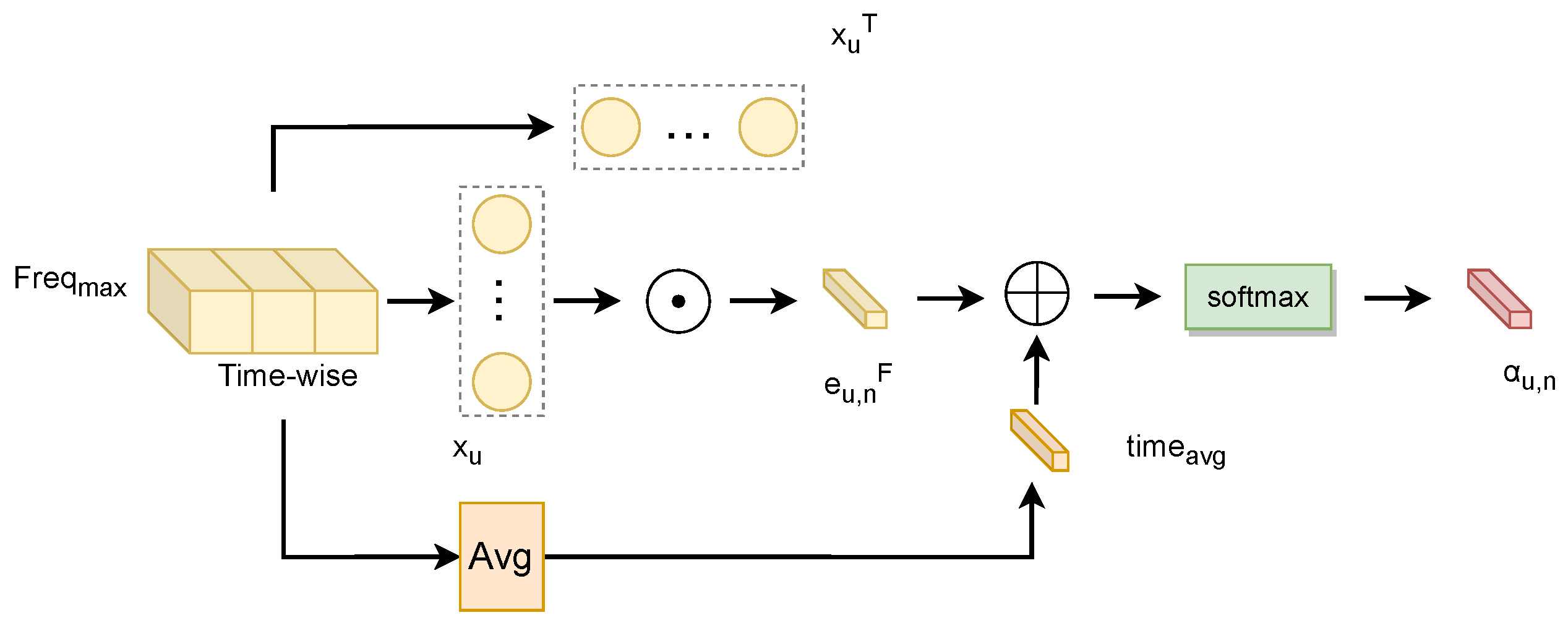
Schematic of attention generation in the GAT layer based on time domain features

This module takes as input the time-domain features corresponding to the maximum frequency magnitude in the time–frequency representation, focusing on modeling the time dimension. It introduces a mean matrix to enhance global statistical information and capture global patterns in the time domain, as shown in Figure 4.

The mean value is computed using Equation (3):

$$tim{e}_{avg}={\displaystyle \frac{1}{N}}\sum _{i=1}^N{X}_i$$

(3)

Equation (4) represents the relationship strength between node $x_u$ and node $x_n$ in its domain:

$$e_{u,n}^T=W_g(x_u\odot x_n)$$

(4)

To integrate the global context, we modify the attention score normalization by incorporating $tim{e}_{avg}$ as an additive bias:

$${\alpha }_{\mathrm{u},\mathrm{n}}^{\mathrm{T}}={\displaystyle \frac{exp({\mathrm{e}}_{\mathrm{u},\mathrm{n}}^{\mathrm{T}}+{\mathrm{time}}_{\mathrm{avg}})}{{\sum }_{\mathrm{w}\in \mathrm{M}\left(\mathrm{u}\right)\cup \left(\mathrm{u}\right)}exp({\mathrm{e}}_{\mathrm{u},\mathrm{w}}^{\mathrm{T}}+{\mathrm{time}}_{\mathrm{avg}})}}$$

(5)

This coefficient ${\alpha }_{\mathrm{u},\mathrm{n}}^{\mathrm{T}}$ determines the relative importance of node ${\mathrm{x}}_{\mathrm{n}}$ in updating the node ${\mathrm{x}}_{\mathrm{u}}$ representation.

By introducing the mean matrix, the model can capture global relationships in temporal data during attention calculation, rather than being limited to local adjacency. Thus, temporal features may encompass broader global patterns and long-term trends. This enhancement improves the module’s ability to recognize long-term changes and global patterns, thereby strengthening the model’s representation of temporal data.

Except the above attention generation part is not the same, the other operations in the GAM are the same in time domain features as in frequency domain features.

For the GAT layer in the GAM based on time domain features, the updated node representation $x_u^{\prime }$ is computed by aggregating its neighboring features weighted by the attention coefficient. Equation (6) represents the node aggregation process in the GAT layer:

$$x_u^{T^{\prime }}=\sum _{w\in M\left(u\right)\cup \left(u\right)}{\alpha }_{u,n}^T{x}_w$$

(6)

$p_{att}$ and $p_{noatt}$ represent the projection of the aggregated and original nodes, respectively:

$$X_u^T=SELU\left(BN(x_u+P_{att}\left(x_u^{\prime }\right)+P_{noatt}\left(x_u^T\right))\right)$$

(7)

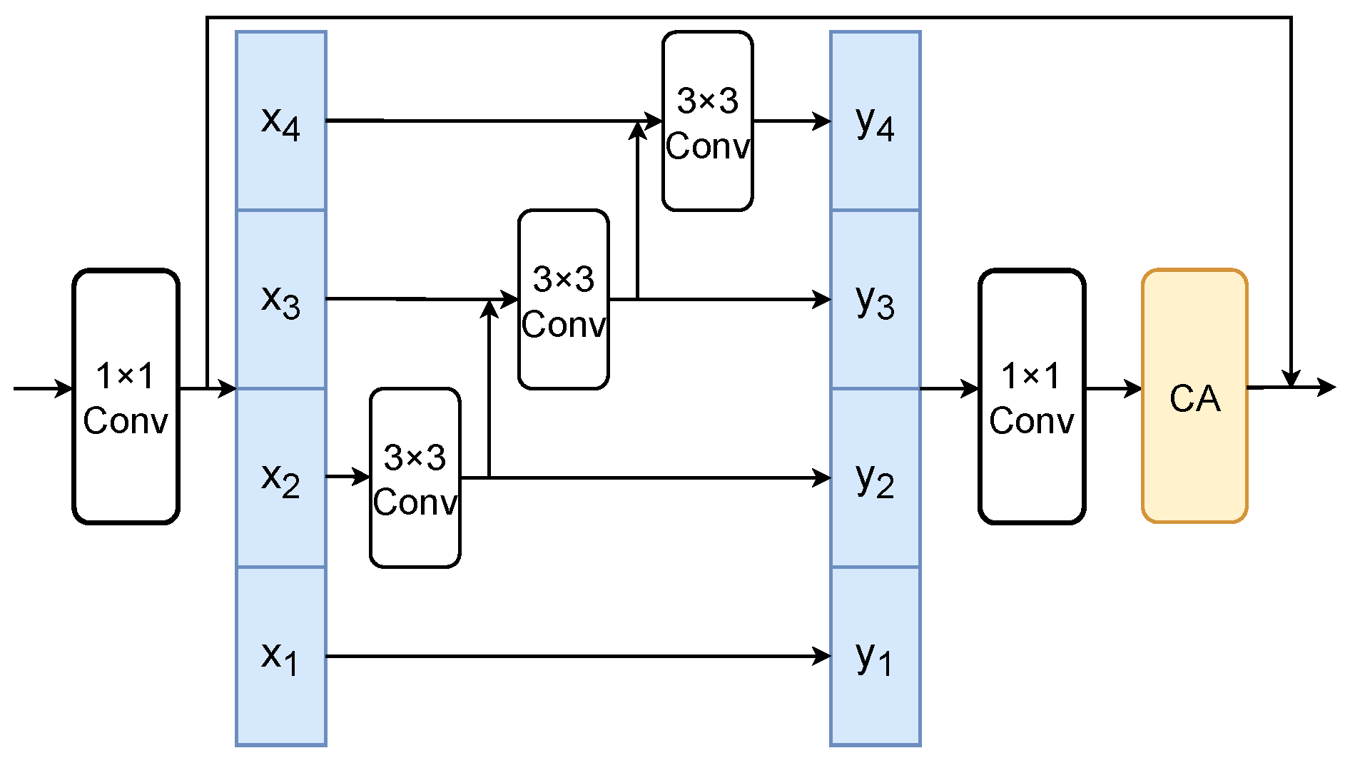
P denotes the projection operation, SELU denotes the scaled exponential linear unit activation function, BN denotes the batch normalization, and the final output of the GAM is $X^T=\{X_1^T,X_2^T,\dots ,X_u^T\}$. In the same way, the final output of the GAM based on frequency domain features is $X^F=\{X_1^F,X_2^F,\dots ,X_u^F\}$.

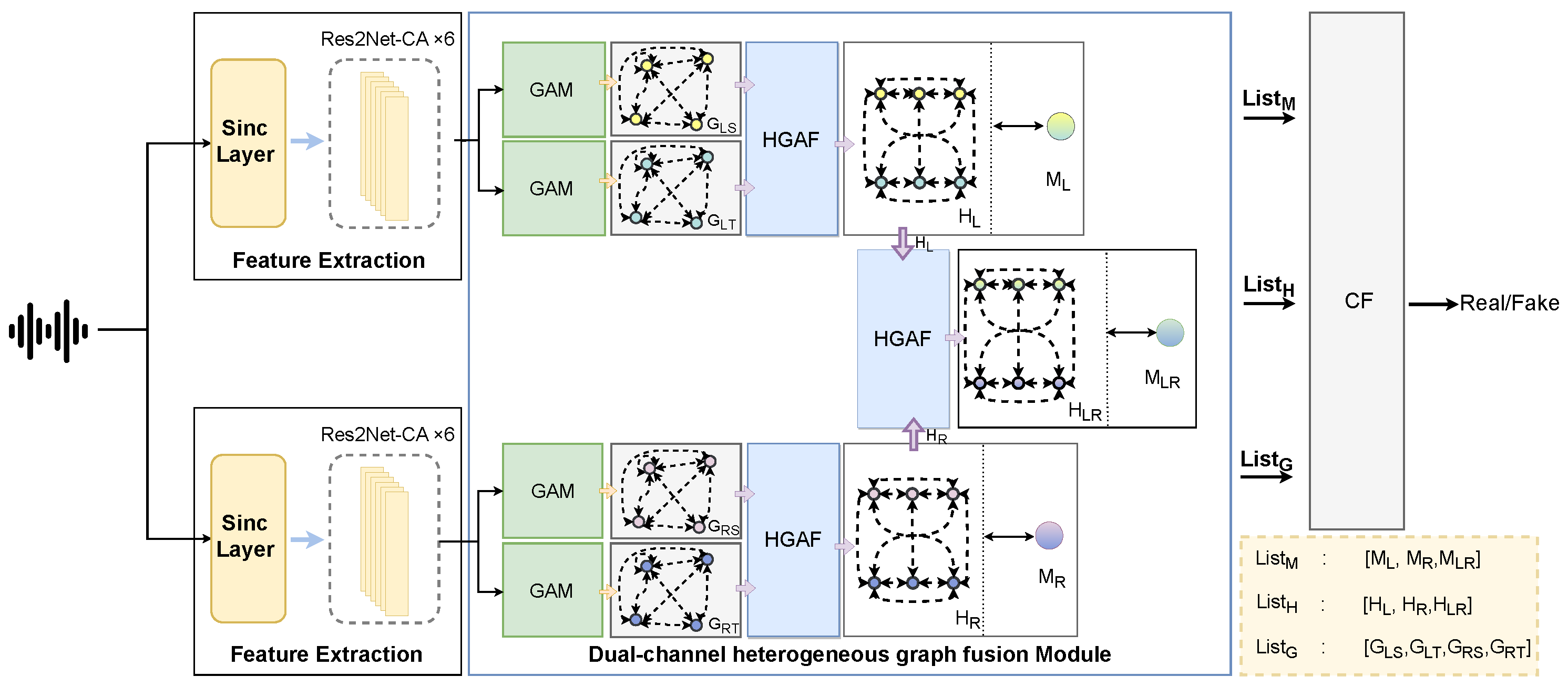
3.3.2. Heterogeneous Graph Attention Fusion Module

Previously, GAM had four views, each of which was represented as follows:

$$c\in \{\{X^T,X^F\},\{Y^T,Y^F\}\}$$

(8)

where $\{X^T,X^F\}$ and $\{Y^T,Y^F\}$ represent the time-domain and frequency-domain views of the left and right vocal tracts, respectively. Although each view contains useful information individually, these views are intrinsically complementary and mutually dependent. The time-domain and frequency-domain features of the same vocal tract describe the same signal from different perspectives. If their mutual relationships are ignored, the representations learned by the model may not be ideal.

(1)

Heterogeneous graph construction

To better exploit the relationships both within and across views, we model them as a heterogeneous graph, where nodes from different views are treated as distinct node types. We adopt a heterogeneous graph attention fusion module (HGAFM) to learn view-specific patterns while simultaneously capturing cross-view dependencies.

Taking the left vocal tract as an example, the heterogeneous graph node aggregation process is introduced. For two views, $X^T\in {\mathbb{R}}^{B\times N_1\times D}$ and $X^F\in {\mathbb{R}}^{B\times N_2\times D}$, where B is the batch size, $N_1$ and $N_2$ represent the number of nodes, and D is the feature dimension. To process the feature information from different views, we project the features from each view into a shared space before treating them as nodes in a heterogeneous graph, as shown in Equation (9):

$$h^{FT}=\left\{\begin{array}{c}\hfill W^T{x}_{Tn},n\in N\left(X^T\right)\\ \hfill W^F{x}_{Fn},n\in N\left(X^F\right)\end{array}\right.$$

(9)

where $N\left(X^T\right)$ and $N\left(X^F\right)$ represent the node sets of the graph structure data $X^T$ and $X^F$, respectively.

(2)

Node aggregation

In the heterogeneous graph $h^{FT}$, the relationship strength $i_{u,n}$ between node $h_u$ and node $h_n$ within its domain is modeled using an attention mechanism, as given by Equation (10).

$$i_{u,n}=W_h(h_u\odot h_n)$$

(10)

The inter-graph attention mechanism adopts a two-node aggregation operation, and the specific operation is shown in Equation (11):

$$i_{u,n}^{\prime }=\left\{\begin{array}{l}{W}_T{i}_{u,n},u,n\in N\left(X^T\right)\\ W_F{i}_{u,n},u,n\in N\left(X^F\right)\\ W_{FT}{i}_{u,n},other\end{array}\right.$$

(11)

Here, the learnable weights $\{W_T,W_F\}\in {\mathbb{R}}^{1\times D}$ are applied to nodes $h_u$ and $h_n$, which are derived from the same set of nodes in $X_T$ or $X_F$, respectively. When the nodes $h_u$ and $h_n$ belong to different node sets, $W_{FT}\in {\mathbb{R}}^{1\times D}$ is applied to node $h_u$ and $h_n$, which are derived from different node sets. Equation (12) computes the attention weights between node $h_u$ and all nodes in its neighborhood $M\left(u\right)$. Then, softmax is used to normalize the attention weights, resulting in ${\alpha }_{u,n}^{FT}$:

$${\alpha }_{u,n}^{FT}={\displaystyle \frac{exp\left(i_{u,n}^{\prime }\right)}{{\sum }_{w\in M\left(u\right)\cup \left(u\right)}exp\left(i_{u,w}^{\prime }\right)}}$$

(12)

where $M\left(u\right)$ is the set of neighboring nodes of node $h_u$, and $i_{u,n}^{\prime }$ is the attention strength between nodes. Finally, the node features are updated as an aggregate of weighted neighbor node features. Equation (13) represents the node aggregation process in the heterogeneous graph attention fusion network:

$$h_u^{{FT}^{\prime }}=\sum _{w\in M\left(u\right)\cup \left(u\right)}{\alpha }_{u,n}^{FT}{h}_w^{FT}$$

(13)

Equation (14) indicates that node $h_u$ is updated by applying a double projection operation on $h_u^{{FT}^{\prime }}$ and $h_u^{FT}$:

$$H_u^{FT}=SELU\left(BN\right(P_{att}\left(h_u^{{FT}^{\prime }}\right)+P_{noatt}\left(h_u^{FT}\right)$$

(14)

The final output of the heterogeneous graph attention fusion module is the heterogeneous graph $H^{FT}=\{H_1^{FT},H_2^{FT},\cdots ,H_u^{FT}\}$.

(3)

Master node information augmentation

In order to enhance the model’s understanding of global information, the heterogeneous graph attention fusion module introduces a master node $s\in {\mathbb{R}}^{B\times 1\times D}$ to capture global information through interaction with all other nodes in the heterogeneous graph, thereby improving the representation of global features. The initial master node is computed as the mean value of $h^{FT}$, as shown in Equation (15):

$$s={\displaystyle \frac{1}{N}}\sum _{i=1}^N{h}_i^{FT}$$

(15)

where N is the total number of nodes in the graph. The master node aggregation process is realized through the self-attention mechanism, where the learnable mapping $W_s$ is used to measure the importance of the master node to other heterogeneous nodes, resulting in the normalized ${\alpha }_s$, as shown in Equation (16):

$${\alpha }_s={\displaystyle \frac{exp\left(W_s(h_u^{FT}\odot s)\right)}{{\sum }_{w\in M\left(u\right)\cup \left(u\right)}exp\left(W_s(h_u^{FT}\odot s)\right)}}$$

(16)

$$s^{\prime }=\sum _{w\in M\left(n\right)\cup \left(n\right)}{\alpha }_s{h}_w^{FT}$$

(17)

Here, $s^{\prime }$ represents the aggregated information enhanced by the master node. Finally, the master node s is obtained by performing a double projection operation on s and $s^{\prime }$, and the calculation process is consistent with Equation (14).

The heterogeneous graph fusion module operates on the left and right vocal channels separately to obtain the left vocal channel fusion view $H_L$, master node $S_L$, and attention map $A_L$, as well as the right vocal channel fusion view $H_R$, master node $S_R$, and attention map $A_R$. Then, the two vocal channel fusion views $H_{LR}$, master node $S_{LR}$, and attention map $A_{LR}$ are obtained by taking $H_L$ and $H_R$ as inputs.

3.4. Channel Fusion Discriminator

To effectively combine features from different sources and enhance the representation of the vocal tract, we introduce the channel fusion discriminator. This module leverages graph pooling and attention mechanisms to selectively fuse important features, thereby improving both local and global feature extraction for better performance. Figure 5 illustrates the architecture of the channel fusion discriminator.

The proposed model employs a grouping strategy to process features from different sources, aiming to retain the critical information from each source. Three feature sets are defined as $U=\{M,H,S\}$, where M, H, and S represent different types of feature sets. The features in M consist of time-domain and frequency-domain views of each vocal tract (e.g., $X^T$, $X^F$, $Y^T$, $Y^F$). The features in H are derived from the relationships between nodes across different views (e.g., $H^L$, $H^R$, $H^{LR}$). The features in S contain the master node information (e.g., $S^L$, $S^R$, $S^{LR}$), which is obtained by fusing the relationships between the various views.

To extract both local and global features from the left and right vocal tract fusion views, the vocal tract fusion discriminator is employed to screen and integrate three sets of features. Each fusion module of the discriminator consists of two graph pooling layers, followed by a series of pooling and concatenation operations, as shown in Figure 5.

The graph pooling layer applies an attention mechanism to weight the node features, enabling the extraction of key information and the reduction of redundancy. For each input feature matrix $h\in {\mathbb{R}}^{B\times N\times D}$ from the feature sets (e.g., $H^L$, $H^R$, $H^{LR}$), where B is the batch size, N is the number of nodes, and D is the feature dimension, the layer first generates the node weights $\omega \in {\mathbb{R}}^{B\times N\times 1}$ through a linear transformation, as shown in Equation (18):

$$\omega =Sigmoid\left(P\right(h\left)\right)$$

(18)

Then, based on a specified ratio k, the most important node features are selected using a topk operation, which ranks the nodes by the importance of their features:

$$h_{new}=topk(\omega \odot h)$$

(19)

Here, k determines the proportion of node features selected from each feature set. The topk operation ranks nodes based on the importance of their features and selects the top $K\times N$ nodes. After two layers of graph pooling, the features are concatenated, followed by max pooling and average pooling operations to aggregate the information:

$$h_{cat}=concat(h_{new1},h_{new2})$$

(20)

$$h_{max}=max\left(\left|h_{cat}\right|\right)$$

(21)

$$h_{avg}={\displaystyle \frac{1}{N}}\sum _{i=1}^N{h}_{cat}$$

(22)

The pooled features are concatenated into a single feature vector, as shown in Equation (23):

$$h_{final}=concat(h_{max},h_{avg})$$

(23)

These fused features from the three sets M, H, and S are then passed through a fully connected layer (MLP) to generate the final prediction:

$$h_{concat}=concat(h_{{final}_M},h_{{final}_H},h_{{final}_S})$$

(24)

$$Z_{pred}=MLP\left(h_{concat}\right)$$

(25)

This approach combines information from all feature sets, enabling the model to learn a more comprehensive representation.

4. Experiments and Analysis

4.1. Dataset Production

The stereo dataset used in this study consists of paired audio data (mono and stereo) from 8 speakers (4 male and 4 female), sampled at 48 kHz, with a total duration of 2 h. The data acquisition process simulates a human auditory scene, where participants engage in spontaneous conversations around a simulated human body model. A binaural microphone-equipped human model was used to record the dataset, with participants walking around the model at varying angles and distances within a 1.5 m radius. This dataset was employed to train the pre-trained stereo conversion model, the M2S converter [22].

The ASVspoof2019 [23] dataset was released by the ASVspoof2019 challenge, which is a large-scale speech dataset, mainly for deception detection in automatic speaker verification (ASV) tasks. This dataset contains two subsets: logical access (LA) and physical access (PA). In this study, we focused on the logical access (LA) subset, which is used to detect spoofing attacks based on acoustic features. The LA subset is further divided into three sets: training, development, and evaluation sets. The training set consists of 2580 genuine speech samples and 22,800 spoofed speech samples, with the spoofed samples generated by six text-to-speech (TTS) and voice conversion (VC) algorithms. Spoofed speech in the training and development sets is generated by six attack algorithms (A01–A06), while the evaluation set contains spoofed speech generated by additional thirteen algorithms (A07–A19). We also evaluated on the ASVspoof2021 LA dataset [24], which is an extended version of ASVspoof2019 with stronger challenges. ASVspoof2021 LA introduces more diverse attack types compared to its predecessor, with the dataset containing 21,000 authentic utterances and 259,000 spoofed utterances. It is important to note that the evaluation set includes attacks generated under different acoustic conditions, for example, background noise and reverberation, simulating real-world deployment scenarios. This dataset is widely used to benchmark the ability of anti-spoofing models to generalize to evolving synthetic speech technologies. The data distribution of ASVspoof 2019 LA and ASVspoof 2021 LA datasets is shown in

Table 1. Data distribution of ASVspoof 2019 LA and ASVspoof 2021 LA datasets.

Dataset	Train		Development		Evaluation
	Real	Fake	Real	Fake	Real	Fake
ASVspoof 2019 LA	2580	22,800	2548	22,296	7355	63,882
ASVspoof 2021 LA	2580	22,800	2548	22,296	14,816	166,750

.

4.2. Implementation Details

To ensure the consistency of the training results, a random seed (seed = 1234) was used to initialize the model parameters. The model was trained for 300 epochs with a batch size of 12, a weight decay rate of 0.0001, and a learning rate of 0.0001. During training, we adopted the ReduceLROnPlateau mechanism, which automatically reduces the learning rate when the validation metrics plateau. The loss function used was weighted cross-entropy loss. The experimental environment consisted of Python 3.8.8, hardware with an RTX 4090 GPU, and CUDA version 11.1.

In order to evaluate the performance of this model in forgery detection, this study mainly used EER (Equal Error Rate) and min-tDCF (Minimum Tandem detection Cost Function) [25] as evaluation indicators. The EER reflects the ability of the model to distinguish between real speech and fake speech, and the lower the EER, the better the recognition performance. min-tDCF is a comprehensive evaluation index based on the detection cost function (DCF). min-tDCF extends the traditional detection cost function (DCF) to deception scenarios by jointly evaluating automatic speaker verification (ASV) and deception countermeasure (CM) systems. Optimizing min-tDCF is helpful to improve the applicability of the model in practical scenarios.

4.3. Module Comparison Experiment

In this section, we experimentally compare the performance of the proposed modules to verify their effectiveness. All experiments were conducted using the ASVspoof2019 dataset and under the same training conditions.

The baseline model (+ResNet18) uses ResNet18 for feature extraction, and a standard graph attention network is employed in the graph attention fusion module. Building on the baseline model, the improved dual-channel heterogeneous graph fusion module (+DHGFM) replaces the standard graph attention network. The final model (+Res2NetCA+DHGFM) integrates the improved Res2NetCA module with the DHGFM, forming the complete model architecture.

Table 2. Module comparison experiment.

Module	EER (%)	Min-tDCF
+Resnet18	3.05	0.10
+DHGFM	2.03	0.065
+Res2netCA+DHGFM	1.64	0.051

Bold denotes the best performance value for each module.

presents a performance comparison of the different module combinations. The baseline model achieved an EER of 3.05% and a min-tDCF of 0.10 on the test set. After adding DHGFM, the performance improved significantly, with EER reduced to 2.03% and min-tDCF reduced to 0.065. Finally, by combining the Res2NetCA module with the improved graph attention network, the performance of the final model was further optimized, achieving an EER of 1.64% and a min-tDCF of 0.051. These results demonstrate the effectiveness of the proposed module combination in improving the detection capability for forged speech.

4.4. Effect of Different Pooling Ratios in the Channel Fusion Discriminator

This section evaluates the effect of different pooling ratios (k values) in the graph pooling operation of the vocal tract fusion discriminator on model performance.

As shown in

Table 3. Impact of k values in graph pooling on model performance.

k	EER (%)	Min-tDCF
0.3	2.66	0.073
0.5	1.64	0.051
0.7	2.79	0.082

Bold denotes the best performance value for each method.

, the experimental results indicate that the choice of the k value significantly impacts the feature extraction and representation capabilities of the model. A small k value may lead to the loss of important feature information, thereby affecting model performance. On the other hand, a large k value increases computational complexity and may not fully exploit the potential features of the graph data. When k = 0.5, the model achieves the best performance in terms of EER and min-tDCF, with values of 1.64% and 0.051, respectively, outperforming all other k configurations. In contrast, for k = 0.3, the EER is 2.66% and min-tDCF is 0.07, where the smaller pooling ratio results in a degradation of model performance. Similarly, for k = 0.7, the EER is 2.79% and min-tDCF is 0.08, and although the pooling ratio is larger, the increased computational complexity limits model performance.

4.5. Comparative Experiments with Existing Methods on the ASVspoof 2019 LA Dataset

Table 4. Results on the ASVspoof2019 LA dataset.

Method	EER (%)	Min-tDCF
PC-DARTS [26]	4.96	0.091
RAW PC-DARTS [27]	1.77	0.0517
RawNet2 [28]	4.66	0.1294
ResNet [29]	3.72	0.119
SafeEar [30]	3.10	0.149
RW-Resnet [31]	2.98	0.082
LCNN [32]	2.76	0.078
HuRawNet2 [33]	1.96	0.139
ours	1.64	0.051

Bold denotes the best performance value for each module.

lists the performance comparison between the proposed method and existing methods based on monaural speech data.

PC-DARTS show limited detection capability, with EERs of 4.96%, respectively. Although the ResNet method, based on amplitude-phase spectrum feature classification, reduces the EER to 3.72%, the min-tDCF remains higher (0.119). SafeEar, which uses acoustic information to avoid semantic leakage, achieves an EER of 3.10% but still lags behind methods that combine full audio features. HuRawNet2, utilizing self-supervised feature extraction, reduces the EER to 1.96%. In contrast, the proposed method, based on dual-channel input, further reduces the EER to 1.64%, which is 0.32% lower than HuRawNet2. Meanwhile, the min-tDCF is maintained at a low level. In summary, under dual-channel input, the proposed method demonstrates superior performance in forged speech detection compared to existing monaural methods.

4.6. Comparative Experiments with Existing Methods on the ASVspoof 2021 LA Dataset

Table 5. Results on the ASVspoof2021 LA dataset.

Method	EER (%)	Min-tDCF
LFCC-GMM [34]	19.30	0.5758
CQCC-GMM [34]	15.62	0.4974
LFCC-LCNN [34]	9.26	0.3446
RAW PC-DARTS [27]	6.43	0.3444
RawNet2 [28]	9.5	0.4257
SafeEar [30]	7.22	0.336
ours	6.76	0.3638

Bold denotes the best performance value for each module.

lists the performance comparison between the proposed method and existing methods based on monaural speech data.

On ASVspoof 2021, our method demonstrates competitive performance. LFCC-GMM, CQCC-GM, and LFCC-LCNN are the baseline systems provided by the ASVspoof 2021 challenge organizers on the LA task. In comparison to LFCC-LCNN, our method achieves a relative reduction of 26.9% and 36.8% in EER and minimum t-DCF on the evaluation dataset. RawNet2 improves the detection ability by modeling the original waveform. However, compared with RAWNet2, the EER and minimum t-DCF of our method on the evaluation dataset are relatively reduced by 28.8% and 36.8%, demonstrating its better performance. Additionally, our approach outperforms SafeEar, achieving a 0.6% relative reduction in EER. Finally, we compared the proposed model with the RAW PC-DARTS. The experimental result showed that the proposed model had comparable performance in forged speech detection, further validating its effectiveness.

4.7. Model Performance Evaluation Across Different Forgery Types

This section uses the ASVspoof2019 LA test set, which contains a variety of forged audio attack types, including two major categories: speech synthesis and voice conversion, as shown in

Table 6. Techniques used for unknown attack types in the ASVspoof2019 LA test set.

Attack Type	Technique Type	Implementation Method
A07	Speech synthesis	vocoder+GAN
A08	Speech synthesis	neural waveform
A09	Speech synthesis	vocoder
A10	Speech synthesis	neural waveform
A11	Speech synthesis	griffin lim
A12	Speech synthesis	neural waveform
A13	Speech synthesis+Voice Conversion	waveform concatenation + wave filtering
A14	Speech synthesis+Voice Conversion	vocoder
A15	Speech synthesis+Voice Conversion	neural waveform
A16	Voice Conversion	waveform concatenation
A17	Voice Conversion	wave filtering
A18	Voice Conversion	vocoder
A19	Voice Conversion	spectral filtering

.

Speech synthesis attacks encompass various methods, including those based on vocoders, Generative Adversarial Networks (GANs), neural waveform generation, the Griffin-Lim algorithm, and others. These methods generate fake audio by simulating the speech production process. Voice conversion attacks, on the other hand, employ techniques such as waveform concatenation, wave filtering, and spectral filtering to manipulate real audio and alter its characteristics, thereby creating counterfeit speech. Each attack method utilizes different technical approaches, ranging from traditional vocoder technology to advanced neural network models, covering diverse paths of audio forgery, from generation to conversion.

Table 7. Results of our method on the ASVspoof 2019 LA evaluation set across different attack types.

Attack Type	EER(%)	min-tDCF
A07	0.75	0.023
A08	0.93	0.031
A09	0.09	0.002
A10	1.11	0.036
A11	0.75	0.025
A12	0.92	0.029
A13	0.61	0.019
A14	0.32	0.01
A15	0.69	0.022
A16	0.97	0.032
A17	4.49	0.137
A18	2.58	0.087
A19	1.23	0.037

presents the performance metrics of the proposed method under different forgery types, evaluated on the ASVspoof2019 LA test set.

Table 7 demonstrates that the model performs well across most forgery attack types. In particular, for attack types such as A09, A13, and A08, the model achieves relatively low EER and min-tDCF values, indicating its strong ability to distinguish between real and forged speech. However, under more complex attack types, such as A17, the model’s performance still requires improvement.

5. Conclusions

In this paper, we propose a dual-channel spoofed speech detection method using a symmetric two-branch framework that integrates Res2Net with coordinate attention and a dual-channel heterogeneous graph fusion module. Experimental results on the ASVspoof2019 and ASVspoof2021 LA datasets demonstrated the superior performance of our approach, which achieved an EER of 1.64% and a Min-tDCF of 0.051 on ASVspoof2019, and an EER of 6.76% with a Min-tDCF of 0.3638 on ASVspoof2021. Our method outperformed existing techniques in terms of detection performance. Future work will focus on optimizing computational efficiency and exploring further enhancements to the fusion strategies.