Reliability Estimation of Stress–Strength Model for Multi-Component System Based on Lomax Distribution Using the Survival Signature

Abstract

In this paper, the stress–strength reliability of complex systems with diverse component types is investigated based on the theoretical framework of survival signatures. Assuming that both the strength and stress of components of the same type follow the Lomax distribution, the maximum likelihood estimation (MLE), maximum spacing estimation (MSPE), and Bayesian estimation for the stress–strength model are derived under the condition that components of the same type have common scale parameters. Subsequently, the 95% Bootstrap-p and Highest Posterior Density confidence intervals for the stress–strength reliability were derived using Monte Carlo simulation. Additionally, since stress cycles are represented by a Poisson process, a dynamic stress–strength model for the system subjected to periodic stresses over the interval $(0,t]$ was developed, together with an approximate computational algorithm for this model. Finally, a simulation experiment was conducted using a system consisting of a total of nine components of three different types to analyze these estimation methods. The findings reveal that MLE exhibits the lowest estimation error, registering merely 0.001 in the case of small-sized samples. Compared with the previous two methods, Bayesian estimation has a relatively larger error. However, in the case of large samples, the error is 0.0112. In addition, the performance and accuracy of the dynamic model were verified through the proposed algorithm. The results indicate that compared with the static model at $t=0$, the error of the algorithm is 0.0464. Overall, the model evaluation results are satisfactory.

1. Introduction

The stress–strength model is a widely utilized framework in system reliability analysis, applicable across various fields such as engineering, geology, oceanography, economics, and materials [1,2,3,4,5]. Its fundamental principle involves comparing the stress imposed on a system or material with its inherent strength. In the context of the stress–strength model, reliability is defined as the probability that the strength of the system or material exceeds the applied stress under given conditions. The classic stress–strength model was first introduced by Birnbaum [6]. Since its inception, numerous researchers have extended and refined the model to better suit the needs of different fields and application scenarios [7,8,9]. By employing the stress–strength model, engineers and designers can gain a deeper understanding of how systems or materials perform under external loads, leading to more rational design and optimization. Additionally, this model aids in predicting and preventing potential failure modes, thereby enhancing the safety and reliability of products.

In reliability engineering, the Lomax distribution has a wide range of applications due to its excellent mathematical and physical properties. The Lomax distribution, also known as the Pareto Type-II distribution, was initially proposed by Lomax for the analysis of failure data in economics [10]. This distribution is particularly suited for datasets that exhibit right-skewed or heavy-tailed characteristics. Over time, with the advancement of scientific research, the Lomax distribution has found applications in various other domains, including reliability engineering [11], transportation engineering [12], telegraph [13], aerospace [14], and computer science [15].

In reliability analysis, the mathematical properties of the Lomax distribution are well-suited to reliability scenarios. Most failures are concentrated in the early stage, but there is a small amount of long-tailed data. Therefore, reliability data, such as equipment lifetime and failure time, are usually right-skewed. The right-skewed characteristic of the Lomax distribution can better fit the long-tail phenomenon in actual data. Compared with other distributions commonly used in reliability, the exponential distribution is unable to model aging or early failures, while the Lomax distribution can model aging by adjusting the shape parameter. In addition, the Weibull distribution has insufficient prediction for extreme events, and extreme events need to be modeled using heavy-tailed distributions. The tail of the Lomax distribution decays more slowly than that of the Weibull distribution, so it can better capture extreme risks. The log-normal distribution has a fast tail decay, which may lead to an underestimation of extreme events. In contrast, the Lomax distribution provides a more conservative estimate of reliability. In engineering practice, the physical meanings of the parameters of the Lomax distribution are well-defined, making it suitable for the modeling of complex systems. Moreover, its ability to account for extreme events endows it with greater value in some crucial fields such as aerospace and nuclear power safety.

A significant amount of research has been conducted on the Lomax distribution. Fitrilia A et al. [16] utilized the E-Bayesian method to estimate the parameters of the Lomax distribution under Type-II right-censored data. Hassan et al. [17] derived the Bayesian estimates of entropy for the Lomax distribution, along with their corresponding confidence intervals, based on linear exponential, squared error, and precautionary loss functions. Dong G et al. [18] estimated the Shannon entropy of the Lomax distribution using noninformative priors. Additionally, the Lomax distribution has gradually been applied to stress–strength reliability models. AlEssa L.A. et al. [19] assumed that the system components follow the Lomax distribution and studied the problem of estimating the distribution parameters of a triple modular redundancy system under step-stress partially accelerated life tests. They employed various estimation methods to analyze the reliability of the system and mean residual lifetime. Hassan M.A. [20] performed statistical inference on reliability for two mutually independent stress and strength variables, assuming a common scale parameter, and derived various point and interval estimates for reliability. Hamad A.M. et al. [21] investigated the stress–strength reliability estimation for the Restricted Exponentiated Lomax distribution under two scenarios when the stress is Y: one scenario involves a single strength $X$, and the other involves dual strengths $X_1$ and $X_2$. In these research findings on stress–strength models of the Lomax distribution, [19] discusses the stress–strength model for k-out-of-n systems, while [20,21] both consider the entire system as a whole. Therefore, from the analysis of existing research, it is discovered that the issue of reliability assessment for stress–strength models of the Lomax distribution in multi-component complex systems with diverse component types has been barely addressed. As a probability distribution, the Lomax distribution has a long-tail characteristic and can effectively describe extreme events, which is particularly important in reliability engineering. However, its application in complex systems has not been fully explored, limiting its potential in stress–strength reliability assessment. Therefore, researching the application of the Lomax distribution in complex systems can enrich the methodology of reliability assessment.

System signature is an effective tool for assessing system reliability, initially introduced by Samaniego F.J. in 1985, and its influence grew substantially with the release of his book “System Signatures and Their Applications in Engineering Reliability” [22]. However, the signature theory requires that the components of the system be independent and identically distributed. To address this, Coolen et al. [23] introduced the concept of survival signature for systems with multiple types of components. This significantly reduces the need for prior information about the system in reliability studies, making it more applicable to practical scenarios. The survival signature theory has significant advantages in the reliability assessment of complex systems. Compared with the methods based on probability statistics [24], it reduces the dependence on the component life distribution and focuses more on the essence of the system structure. In contrast to machine learning methods [25], it has stronger interpretability and lower data requirements. When compared with system dynamics methods [26], it is simpler and more efficient in calculations and directly links the system structure with reliability. In comparison with multi-attribute decision-making methods [27], it focuses on the core assessment of reliability and provides clear system reliability indicators. These features make it more practical and efficient in the reliability analysis of complex systems. Bai X et al. [28] conducted statistical inference on the stress–strength reliability of a system with bounded strength, using the survival signature theory for a three-parameter exponentiated Weibull distribution with unequal scale and shape parameters. Bai X et al. [29] proposed a new stress–strength model for multi-state systems composed of multiple types of multi-state components. In the case where all types of components are exposed to the same set of dependent stresses, they used an improved generalized survival signature to perform statistical inference on stress–strength reliability. Jana N et al. [30], under progressive Type-II censoring, investigated the reliability of a stress-strength system with multiple types of components using the signature approach for a two-parameter inverse Weibull distribution, deriving various point estimators and confidence intervals. Liu Y et al. [31] studied the stress–strength reliability of multi-state systems based on generalized survival signatures and derived the expressions for stress–strength reliability in both discrete and continuous cases. However, in practical problems, the strength of some components and systems can change over time, and the stress acting on components or systems is a cumulative process. Yet, an analysis of many current research findings from [28] to [31] reveals that they are all static stress–strength reliability models. Research on dynamic stress–strength reliability models for systems with multiple types of components has not been seen. However, in engineering practice, the stress and strength of many components will degrade over time due to factors such as material fatigue and environmental corrosion. Static models cannot capture such dynamic changes, which may lead to inaccurate reliability assessment results and affect the safety and reliability of the system. Therefore, extending the stress–strength model to a dynamic one can more realistically reflect the actual operating conditions of components and improve the accuracy and practicality of the assessment.

In conclusion, this paper has two main research objectives. One is to discuss the estimation of the model parameters and the stress–strength reliability of complex multi-component systems where both the stress and strength variables follow the Lomax distribution. The other is to introduce the time variable into the static stress–strength model and complete the expansion of the model from static to dynamic.

Consequently, in response to the first research objective, the content of the study is that when the stress and strength variables corresponding to different types of components in the system all follow the Lomax distribution, where the Lomax distribution parameters vary across different types of components, the stress–strength model of such complex systems is derived utilizing the survival signature theory. Then, based on different parameter estimation methods, the parameter estimation results for each type of component and the estimates of stress–strength reliability are provided, and the accuracies of these estimation methods are compared. In addition, the sensitivity of the model to each parameter and sample size under different parameter estimation methods needs to be analyzed and compared.

The second research content of this paper is to solve the problem of dynamic stress-strength estimation for the system. By leveraging the relevant theories of stochastic processes, the time variable is introduced into the stress–strength model derived from the first research question, and an estimation algorithm for the model is presented. Subsequently, the accuracy of the algorithm is determined by comparing it with the static model, and the sensitivity of the model to hyperparameters is analyzed.

2. Model Description

Assume that the system has $K$ types of components, where $K\ge 2$. $M_k$ represents the number of components of type $k$, where $k=1, 2,\dots ,K$ and $m=\sum _{k=1}^K{M}_k$. Let the state vector of the system be defined as $\mathit{s}=({\mathit{s}}^1,{\mathit{s}}^2,\dots ,{\mathit{s}}^{\mathit{K}})$, where ${\mathit{s}}^{\mathit{k}}=\left(s_1^k, s_2^k, \dots , s_{M_k}^k\right)\in {\left\{0, 1\right\}}^{M_k}$. $s_i^k (i=0, 1, \dots , M_k)$ represents the state of the $i$th component of type $k$, where $s_i^k=0$ indicates that the $i$th component of type $k$ has failed, and $s_i^k=1$ indicates that the $i$th component is functioning. $l_k$ represents the number of components of type $k$ that are in the working state, where $l_k=0, 1, \dots , M_k$. $\varphi$ is the structure function of the system, with $\varphi =1$ indicating that the system is operational and $\varphi =0$ otherwise. The survival signature of the system, $\Phi (l_1, l_2, \dots , l_K)$, is defined as the probability that the system is functioning, given that, for each type $k$, $l_k$ out of $M_k$ components are functional. It can be formulated as follows:

$$\Phi \left(l_1, l_2, \dots , l_K\right)=\left[\prod _{k=1}^K{\left(\begin{array}{c}{M}_k\\ l_k\end{array}\right)}^{-1}\right]\times \sum _{\mathit{s}\in S_{l_1, l_2, \dots , l_K}}\varphi \left(\mathit{s}\right)$$

(1)

where $S_{l_1, l_2, \dots , l_K}$ represents the set of all state vectors for the whole system at which ${\sum }_{i=1}^{M_k}{s}_i^k=l_k$ for $k=1, 2, \dots , K$ [27]. In Equation (1), $\prod _{k=1}^K\left(\begin{array}{c}{M}_k\\ l_k\end{array}\right)$ calculates the total number of all possible combinations when there are $l_1, l_2, \dots , l_K$ working components among the components of types $1, 2, \dots , K$ respectively. In the classical probability model, it corresponds to the total number of samples. $\sum _{\mathit{s}\in S_{l_1, l_2, \dots , l_K}}\varphi \left(\mathit{s}\right)$ calculates the number of combinations that enable the system to be in a normal operating state. In the classical probability model, it corresponds to the number of samples of the event “the system is in an operating state”. Therefore, Equation (1) represents the probability of the event “the system is in an operating state”.

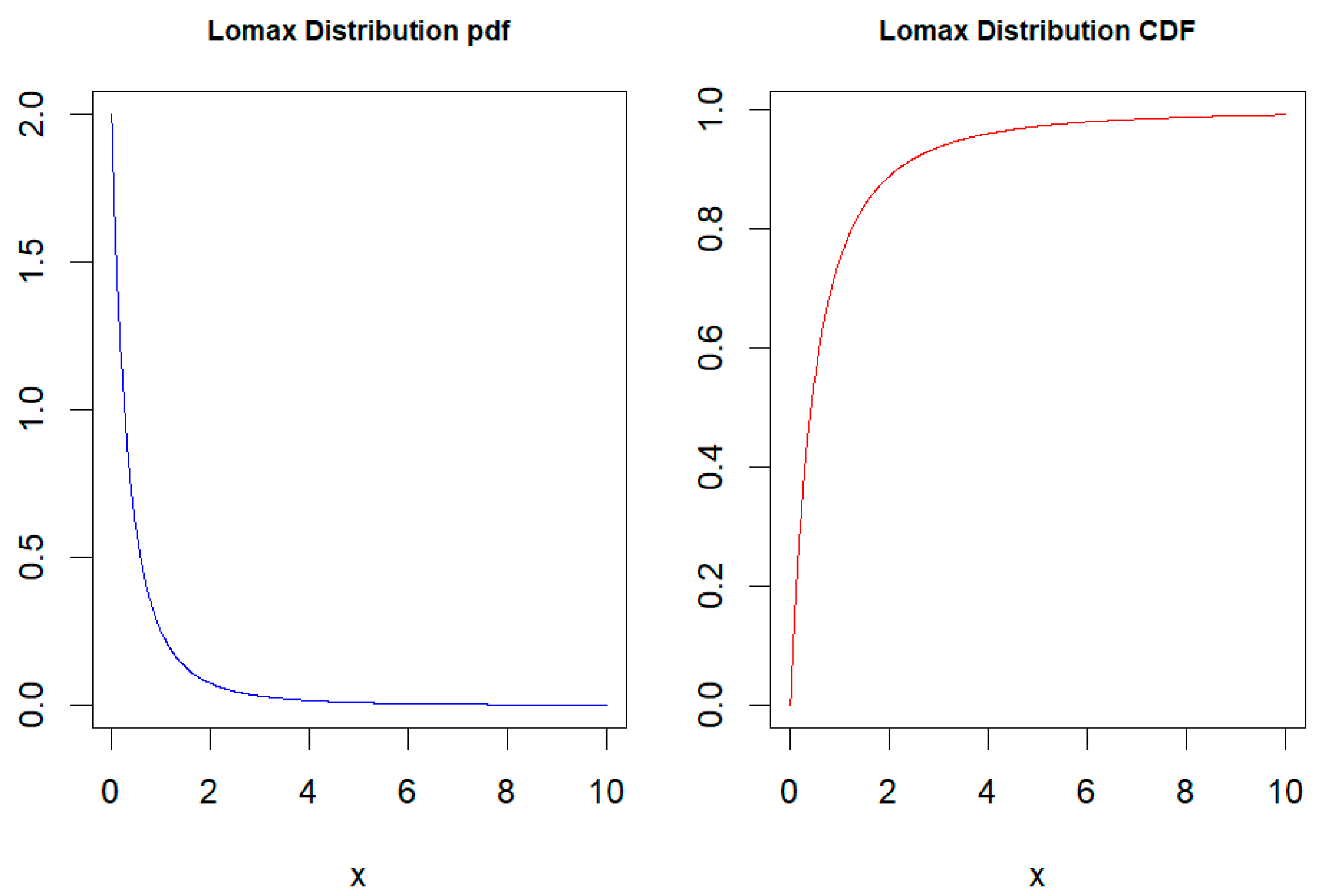
Within the system, the strength variables of the various components are mutually independent, the stress variables experienced by each component are independently distributed, and the stress and strength variables are also independent of each other. All the strength variables of the components and the stress variables they experience follow the Lomax distribution. If random variable $X$ follows the Lomax distribution [32], its probability density function (pdf) can be expressed as follows:

$$f\left(x;\theta ,\lambda \right)=\theta \lambda {(1+\lambda x)}^{-(\theta +1)}, x>0$$

(2)

the cumulative distribution function (CDF) can be depicted as follows:

$$F\left(x;\theta ,\lambda \right)=1-{\left(1+\lambda x\right)}^{-\theta }, x>0$$

(3)

where $\theta >0$ is the shape parameter and $\lambda >0$ is the scale parameter, denoted as $X~L(\theta ,\lambda )$.

Figure 1 shows the pdf and CDF of $L(2, 1)$. From the figure, it can be seen that the Lomax distribution exhibits right-skewness and heavy-tailed characteristics.

Let the random variables $X_k$ and $Y_k (k=1, 2, \dots , K)$ represent the strength and the stress endured by the components of type $k$. From the assumption of the independence between stress variables and strength variables, it can be known that $X_k$ and $Y_k$ are independent of each other. Given that the strength variable $X_k~L\left({\theta }_k,{\lambda }_k\right)$, where the pdf denoted as $f_{X_k}\left(x_k\right)$ and the CDF is denoted as $F_{X_k}\left(x_k\right)$. Similarly, the stress variable $Y_k~L\left({\beta }_k,{\lambda }_k\right)$, with its pdf and CDF denoted as $f_{Y_k}\left(y_k\right)$ and $F_{Y_k}\left(y_k\right)$, respectively. Here, ${\lambda }_k$ is the common scale parameter, ${\theta }_k$ and ${\beta }_k$ are the shape parameters corresponding to the strength and stress variables, respectively, and all these parameters are unknown. $N_k$ represents the number of components of type $k$ that satisfy the condition $X_k>Y_k$, where $N_k=0, 1, 2, \dots , M_k$. Therefore, the stress–strength reliability of the system can be defined as follows:

$$\begin{array}{ll}{R}_{ss}& ={\displaystyle \sum _{l_1=0}^{M_1}}{\displaystyle \sum _{l_2=0}^{M_2}}\cdots {\displaystyle \sum _{l_K=0}^{M_K}}\Phi \left(l_1, l_2, \dots , l_K\right)P\left({\displaystyle \bigcap _{k=\mathrm{1,\; 2}, \dots , K}}\left\{N_k=l_k\right\}\right)\\ & ={\displaystyle \sum _{l_1=0}^{M_1}}{\displaystyle \sum _{l_2=0}^{M_2}}\cdots {\displaystyle \sum _{l_K=0}^{M_K}}\Phi \left(l_1, l_2, \dots , l_K\right){\displaystyle \prod _{k=1}^K}\left(\begin{array}{c}{M}_k\\ l_k\end{array}\right)J_k, \end{array}$$

(4)

where $J_k={\int }_0^{\mathrm{\infty }}{\left[1-F_{X_k}\left(y_k\right)\right]}^{l_k}{\left[F_{X_k}\left(y_k\right)\right]}^{M_k-l_k}{f}_{Y_k}\left(y_k\right)\mathrm{d}{y}_k$ [33].

From the distribution types of $X_k$ and $Y_k$, we can infer that

$$J_k={\int }_0^{\infty }{\left[{(1+{\lambda }_k{y}_k)}^{-{\theta }_k}\right]}^{l_k}{\left[1-{(1+{\lambda }_k{y}_k)}^{-{\theta }_k}\right]}^{M_k-l_k}·{\beta }_k{\lambda }_k{(1+{\lambda }_k{y}_k)}^{-{(\beta }_k+1)}\mathrm{d}{y}_k,$$

let $1+{\lambda }_k{y}_k=z_k$, $J_k$ is derived as follows:

$$\begin{array}{cc}{J}_k& ={\displaystyle \sum _{i_k=0}^{M_k-l_k}}\left(\begin{array}{c}{M}_k-l_k\\ i_k\end{array}\right){(-1)}^{i_k}{\beta }_k{\int }_1^{\infty }{z_k}^{-{\theta }_k\left(l_k+i_k\right)-{\beta }_k-1}\mathrm{d}{z}_k\\ & ={\displaystyle \sum _{i_k=0}^{M_k-l_k}}\left(\begin{array}{c}{M}_k-l_k\\ i_k\end{array}\right){\displaystyle \frac{{\left(-1\right)}^{i_k}{\beta }_k}{{\theta }_k\left(l_k+i_k\right)+{\beta }_k}}, \end{array}$$

(5)

substituting (5) into (4), the stress–strength reliability is expressed as follows:

$$R_{ss}=\sum _{l_1=0}^{M_1}\sum _{l_2=0}^{M_2}\cdots \sum _{l_K=0}^{M_K}\left[\Phi \left(l_1, l_2, \dots , l_K\right)\prod _{k=1}^K\left(\begin{array}{c}{M}_k\\ l_k\end{array}\right)\sum _{i_k=0}^{M_k-l_k}\left(\begin{array}{c}{M}_k-l_k\\ i_k\end{array}\right){\displaystyle \frac{{\left(-1\right)}^{i_k}{\beta }_k}{{\theta }_k\left(l_k+i_k\right)+{\beta }_k}}\right]$$

(6)

3. Point Estimation

3.1. Maximum Likelihood Estimation

Suppose $X_{k,1}, X_{k,2}, \dots , X_{k,n_k}$ is a set of samples from $X_k$, and the observed values of these samples are $x_{k,1}, x_{k,2}, \dots , x_{k,n_k}$. Similarly, $Y_{k,1}, Y_{k,2}, \dots , Y_{k,m_k}$ represents a set of samples from $Y_k$, with the observed values being $y_{k,1}, y_{k,2}, \dots , y_{k,m_k}$. Since these variables are independent of each other, the likelihood function of the samples is as follows:

$$l_k({\theta }_k,{\beta }_k,{\lambda }_k;{\mathit{x}}_k, {\mathit{y}}_k)=\prod _{i=1}^{n_k}{f}_{X_k}\left(x_{k,i};{\theta }_k,{\lambda }_k\right)\prod _{j=1}^{m_k}{f}_{Y_k}\left(y_{k,j};{\beta }_k,{\lambda }_k\right)$$

(7)

The log-likelihood and the score functions are expressed as follows:

$$\begin{gathered} \ln l_k({\theta }_k,{\beta }_k,{\lambda }_k;{\mathit{x}}_k, {\mathit{y}}_k)=n_k\ln {\theta }_k+m_k\ln {\beta }_k+\left(n_k+m_k\right)\ln {\lambda }_k \\ -\left({\theta }_k+1\right){\displaystyle \sum _{i=1}^{n_k}}\ln \left(1+{\lambda }_k{x}_{k,i}\right)-\left({\beta }_k+1\right)\sum _{j=1}^{m_k}\ln \left(1+{\lambda }_k{y}_{k,j}\right) \end{gathered}$$

(8)

$$\left\{\begin{array}{c}{\displaystyle \frac{\partial l_k}{\partial {\theta }_k}}={\displaystyle \frac{n_k}{{\theta }_k}}-{\displaystyle \sum _{i=1}^{n_k}}\ln \left(1+{\lambda }_k{x}_{k,i}\right)=0\\ {\displaystyle \frac{\partial l_k}{\partial {\beta }_k}}={\displaystyle \frac{m_k}{{\beta }_k}}-{\displaystyle \sum _{j=1}^{m_k}}\ln \left(1+{\lambda }_k{y}_{k,j}\right)=0\\ {\displaystyle \frac{\partial l_k}{\partial {\lambda }_k}}={\displaystyle \frac{n_k+m_k}{{\lambda }_k}}-\left({\theta }_k+1\right){\displaystyle \sum _{i=1}^{n_k}}{\displaystyle \frac{x_{k,i}}{1+{\lambda }_k{x}_{k,i}}}-\left({\beta }_k+1\right){\displaystyle \sum _{j=1}^{m_k}}{\displaystyle \frac{y_{k,j}}{1+{\lambda }_k{y}_{k,j}}}=0\end{array}\right.,$$

(9)

where ${\mathit{x}}_k=(x_{k,1}, x_{k,2}, \dots , x_{k,n_k})$, ${\mathit{y}}_k=(y_{k,1}, y_{k,2}, \dots , y_{k,m_k})$ and $k=\mathrm{1,\; 2}, \dots , K$. Taking the partial derivatives of the log-likelihood function yields the following system of nonlinear equations.

The MLE for the parameters ${\theta }_k, {\beta }_k$ and ${\lambda }_k$ are expressed as follows:

$${\widehat{\theta }}_k=n_k{\left[{\displaystyle \sum _{i=1}^{n_k}}\ln (1+{\widehat{\lambda }}_k{x}_{k,i})\right]}^{-1},$$

(10)

$${\widehat{\beta }}_k=m_k{\left[{\displaystyle \sum _{j=1}^{m_k}}\ln \left(1+{\widehat{\lambda }}_k{y}_{k,j}\right)\right]}^{-1},$$

(11)

$${\widehat{\lambda }}_k=\left(n_k+m_k\right){\left[\left({\widehat{\theta }}_k+1\right){\displaystyle \sum _{i=1}^{n_k}}{\displaystyle \frac{x_{k,i}}{1+{\widehat{\lambda }}_k{x}_{k,i}}}+\left({\widehat{\beta }}_k+1\right){\displaystyle \sum _{j=1}^{m_k}}{\displaystyle \frac{y_{k,j}}{1+{\widehat{\lambda }}_k{y}_{k,j}}}\right]}^{-1}.$$

(12)

The calculations for the expressions of ${\widehat{\theta }}_k$ and ${\widehat{\beta }}_k$ both rely on ${\widehat{\lambda }}_k$. Therefore, ${\widehat{\lambda }}_k$ is first obtained using the Newton-Raphson algorithm, after which it is substituted into Equations (10) and (11) to determine ${\widehat{\theta }}_k$ and ${\widehat{\beta }}_k$. Finally, leveraging the invariance property of the MLE, ${\widehat{\theta }}_k$, ${\widehat{\beta }}_k$ and ${\widehat{\lambda }}_k$ are incorporated into Equation (6) to derive the MLE of the stress–strength reliability ${\widehat{R}}_{ss}$.

3.2. Maximum Spacing Estimation

Maximum spacing estimation (MSPE), proposed by Cheng and Amin [34], is an estimation method that can serve as an alternative to MLE. MSPE possesses all the desirable properties of MLE, such as consistency, asymptotic normality, efficiency, and invariance. In subsequent research, Ranneby [35] derived the computational method for MSPE by approximating the Kullback–Leibler divergence. The MSPE for parameter $\mathit{\theta }$ can be obtained by maximizing $M\left(\mathit{\theta }\right)$.

$$M\left(\mathit{\theta }\right)={\displaystyle \sum _{i=1}^{n+1}}\ln \left[F\left(x_{\left(i\right)},\mathit{\theta }\right)-F\left(x_{\left(i-1\right)},\mathit{\theta }\right)\right],$$

(13)

where $x_{\left(i\right)}$ represents the $i$th order statistics of the samples, and $F\left(x\right)$ is the CDF.

The order statistics corresponding to the strength samples $X_{k,1}, X_{k,2}, \dots , X_{k,n_k}$ from the components of type $k$ are denoted as $X_{k,\left(1\right)}, X_{k,\left(2\right)}, \dots , X_{k,\left(n_k\right)}$. Similarly, the order statistics corresponding to the stress samples $Y_{k,1}, Y_{k,2}, \dots , Y_{k,m_k}$ are denoted as $Y_{k,\left(1\right)}, Y_{k,\left(2\right)}, \dots , Y_{k,\left(m_k\right)}$. Their observed values are represented by $x_{k,\left(1\right)}, x_{k,\left(2\right)}, \dots , x_{k,\left(n_k\right)}$ and $y_{k,\left(1\right)},y_{k,\left(2\right)},\dots ,y_{k,\left(m_k\right)}$. From Equation (13), it follows that

$$\begin{gathered} \begin{array}{cc}M\left({\theta }_k,{\beta }_k,{\lambda }_k\right)& ={\displaystyle \sum _{r_1=1}^{n_k+1}}\ln \left[F_{X_k}\left(x_{k,\left(r_1\right)}\right)-F_{X_k}\left(x_{k,\left(r_1-1\right)}\right)\right]+{\displaystyle \sum _{r_2=1}^{m_k+1}}\ln \left[F_{Y_k}\left(y_{k,\left(r_2\right)}\right)-F_{Y_k}\left(y_{k,\left(r_2-1\right)}\right)\right]\\ & ={\displaystyle \sum _{r_1=1}^{n_k+1}}\ln \left[{\left(1+{\lambda }_k{x}_{k,\left(r_1-1\right)}\right)}^{-{\theta }_k}-{\left(1+{\lambda }_k{x}_{k,\left(r_1\right)}\right)}^{-{\theta }_k}\right]\end{array} \\ +{\displaystyle \sum _{r_2=1}^{m_k+1}}\ln \left[{\left(1+{\beta }_k{y}_{k,\left(r_2-1\right)}\right)}^{-{\beta }_k}-{\left(1+{\beta }_k{y}_{k,\left(r_2\right)}\right)}^{-{\beta }_k}\right],\left(k=\mathrm{1,2},\dots ,K\right) \end{gathered}$$

(14)

Let the MSPEs corresponding to the parameters ${\theta }_k, {\beta }_k, {\lambda }_k$ that maximize $M\left({\theta }_k, {\beta }_k, {\lambda }_k\right)$ be ${\tilde{\theta }}_k, {\tilde{\beta }}_k, {\tilde{\lambda }}_k$, respectively. The partial derivatives of $M\left({\theta }_k, {\beta }_k, {\lambda }_k\right)$ with respect to parameters ${\theta }_k, {\beta }_k, {\lambda }_k$ are as follows:

$$\begin{array}{l}{\displaystyle \frac{\partial M}{\partial {\theta }_k}}={\displaystyle \sum _{r_1=1}^{n_k+1}}{\displaystyle \frac{{\left(1+{\lambda }_k{x}_{k,\left(r_1-1\right)}\right)}^{-{\theta }_k}\ln \left(1+{\lambda }_k{x}_{k,\left(r_1-1\right)}\right)-{\left(1+{\lambda }_k{x}_{k,\left(r_1\right)}\right)}^{-{\theta }_k}\ln \left(1+{\lambda }_k{x}_{k,\left(r_1\right)}\right)}{{\left(1+{\lambda }_k{x}_{k,\left(r_1-1\right)}\right)}^{-{\theta }_k}-{\left(1+{\lambda }_k{x}_{k,\left(r_1\right)}\right)}^{-{\theta }_k}}}=0\\ {\displaystyle \frac{\partial M}{\partial {\beta }_k}}={\displaystyle \sum _{r_2=1}^{m_k+1}}{\displaystyle \frac{{\left(1+{\beta }_k{y}_{k,\left(r_2-1\right)}\right)}^{-{\beta }_k}\ln \left(1+{\beta }_k{y}_{k,\left(r_2-1\right)}\right)-{\left(1+{\beta }_k{y}_{k,\left(r_2\right)}\right)}^{-{\beta }_k}\ln \left(1+{\beta }_k{y}_{k,\left(r_2\right)}\right)}{{\left(1+{\beta }_k{y}_{k,\left(r_2-1\right)}\right)}^{-{\beta }_k}-{\left(1+{\beta }_k{y}_{k,\left(r_2\right)}\right)}^{-{\beta }_k}}}=0\\ {\displaystyle \frac{\partial M}{\partial {\lambda }_k}}={\displaystyle \sum _{r_1=1}^{n_k+1}}{\displaystyle \frac{{{\theta }_k{x}_{k,\left(r_1\right)}\left(1+{\lambda }_k{x}_{k,\left(r_1\right)}\right)}^{-{\theta }_k-1}-{\theta }_k{x_{k,\left(r_1-1\right)}\left(1+{\lambda }_k{x}_{k,\left(r_1-1\right)}\right)}^{-{\theta }_k-1}}{{\left(1+{\lambda }_k{x}_{k,\left(r_1-1\right)}\right)}^{-{\theta }_k}-{\left(1+{\lambda }_k{x}_{k,\left(r_1\right)}\right)}^{-{\theta }_k}}}\\ +{\displaystyle \sum _{r_2=1}^{m_k+1}}{\displaystyle \frac{{{\beta }_k{y}_{k,\left(r_2\right)}\left(1+{\beta }_k{y}_{k,\left(r_2\right)}\right)}^{-{\beta }_k-1}-{\beta }_k{y}_{k,\left(r_{2-1}\right)}{\left(1+{\beta }_k{y}_{k,\left(r_2-1\right)}\right)}^{-{\beta }_k-1}}{{\left(1+{\beta }_k{y}_{k,\left(r_2-1\right)}\right)}^{-{\beta }_k}-{\left(1+{\beta }_k{y}_{k,\left(r_2\right)}\right)}^{-{\beta }_k}}}=0\end{array}$$

(15)

The system of nonlinear Equations does not have an analytical solution. Therefore, the L-BFGS-B algorithm can be used to find the maximum value of the function $M\left({\theta }_k, {\beta }_k, {\lambda }_k\right)$ to obtain the MSPEs of the parameters ${\theta }_k, {\beta }_k, {\lambda }_k$, denoted as ${\tilde{\theta }}_k, {\tilde{\beta }}_k, {\tilde{\lambda }}_k$. Substituting these values into Equation (6) yields the MSPE of the stress–strength reliability.

3.3. Bayesian Estimation

As an equally important method compared to classical statistical analysis, the Bayesian approach has received widespread attention in recent decades. In Bayesian statistics, the Gamma distribution is often used as a conjugate prior for the parameters of the exponential family distribution. Its advantages include mathematical convenience, flexibility, and suitability for non-negative parameters, which make the Bayesian updating process simpler and more efficient. Therefore, in this section, the Gamma distribution is chosen as the prior distribution for the parameters to study the stress–strength reliability under the squared loss function. Assum that ${\theta }_k~\Gamma \left(a_{k,1}, b_{k,1}\right)$, ${\beta }_k~\Gamma \left(a_{k,2}, b_{k,2}\right)$ and ${\lambda }_k~\Gamma (a_{k,3}, b_{k,3})$, where $a_{k,1}$, $a_{k,2}$ and $a_{k,3}$ are shape parameters, and $b_{k,1}$, $b_{k,2}$, and $b_{k,3}$ are scale parameters. Suppose the prior distributions of the parameters are independent, and the joint posterior density function is as follows:

$${\pi }_k\left({\theta }_k, {\beta }_k,{\lambda }_k|{\mathit{x}}_k,{\mathit{y}}_k\right)={\displaystyle \frac{{\pi }_k\left({\theta }_k\right){\pi }_k\left({\beta }_k\right){\pi }_k\left({\lambda }_k\right)l_k\left({\theta }_k,{\beta }_k,{\lambda }_k\right)}{{\int }_0^{\infty }{\int }_0^{\infty }{\int }_0^{\infty }{\pi }_k\left({\theta }_k\right){\pi }_k\left({\beta }_k\right){\pi }_k\left({\lambda }_k\right)l_k\left({\theta }_k,{\beta }_k,{\lambda }_k\right)\mathrm{d}{\theta }_k\mathrm{d}{\beta }_k\mathrm{d}{\lambda }_k}},$$

(16)

$$\begin{gathered} {\pi }_k\left({\theta }_k, {\beta }_k,{\lambda }_k|{\mathit{x}}_k,{\mathit{y}}_k\right)\propto {\theta }_k^{a_{k,1}+n_k-1}{\beta }_k^{a_{k,2}+m_k-1}{\lambda }_k^{a_{k,3}+n_k+m_k-1}{e}^{-{\theta }_k[{\sum }_{i=1}^{n_k}\ln \left(1+{\lambda }_k{x}_{k,i}\right)+b_{k,1}]} \\ \times e^{-{\beta }_k[{\sum }_{j=1}^{m_k}\ln (1+{\lambda }_k{y}_{k,j})+b_{k,2}]}{e}^{-[b_{k,3}{\lambda }_3+{\sum }_{i=1}^{n_k}\ln (1+{\lambda }_k{x}_{k,i})+{\sum }_{j=1}^{m_k}\ln (1+{\lambda }_k{y}_{k,j})]}, \end{gathered}$$

(17)

When all the parameters are independent, the marginal posterior densities for ${\theta }_k$, ${\beta }_k$, and ${\lambda }_k$ are given by the following expressions:

$${\pi }_k\left({\theta }_k|{{\beta }_k,{\lambda }_k,\mathit{x}}_k,{\mathit{y}}_k\right)\propto \Gamma \left(a_{k,1}+n_k, {\displaystyle \sum _{i=1}^{n_k}}\ln \left(1+{\lambda }_k{x}_{k,i}\right)+b_{k,1}\right),$$

(18)

$${\pi }_k\left({\beta }_k|{{\theta }_k,{\lambda }_k,\mathit{x}}_k,{\mathit{y}}_k\right)\propto \Gamma \left(a_{k,2}+m_k,{\displaystyle \sum _{j=1}^{m_k}}\ln \left(1+{\lambda }_k{y}_{k,j}\right)+b_{k,2}\right),$$

(19)

$${\pi }_k\left({\lambda }_k|{{\theta }_k,{\beta }_k,\mathit{x}}_k,{\mathit{y}}_k\right)\propto {\lambda }_k^{a_{k,3}+n_k+m_k-1}{e}^{-[b_{k,3}{\lambda }_3+{\sum }_{i=1}^{n_k}\ln (1+{\lambda }_k{x}_{k,i})+{\sum }_{j=1}^{m_k}\ln (1+{\lambda }_k{y}_{k,j})]}.$$

(20)

Under the squared loss function, the Bayesian estimation of $R_{ss}$ is as follows:

$$\begin{array}{c}{\widehat{R}}_{ss}^B={\displaystyle \sum _{l_1=0}^{M_1}}{\displaystyle \sum _{l_2=0}^{M_2}}\cdots {\displaystyle \sum _{l_K=0}^{M_K}}\left[\Phi \left(l_1,l_2,\dots ,l_K\right){\displaystyle \prod _{k=1}^K}\left(\begin{array}{c}{M}_k\\ l_k\end{array}\right){\displaystyle \sum _{i_k=0}^{M_k-l_k}}\left(\begin{array}{c}{M}_k-l_k\\ i_k\end{array}\right)\right.\\ \times \left.{\int }_0^{\infty }{\int }_0^{\infty }{\int }_0^{\infty }{\displaystyle \frac{{\left(-1\right)}^{i_k}{\beta }_k}{{\theta }_k\left(l_k+i_k\right)+{\beta }_k}}·{\pi }_k\left({\theta }_k, {\beta }_k,{\lambda }_k|{\mathit{x}}_k,{\mathit{y}}_k\right)\mathrm{d}{\theta }_k\mathrm{d}{\beta }_k\mathrm{d}{\lambda }_k\right]. \end{array}$$

(21)

Equation (21) does not have an analytical solution, so its approximate solution can be obtained using the Markov Chain Monte Carlo (MCMC) method. First, set the iterative initial value $s$ to 1, and assume that the prior distributions of parameters ${\theta }_k$, ${\beta }_k$, and ${\lambda }_k$ are all Gamma distributions (prior parameters are known). Since the posterior marginal distributions of parameters ${\theta }_k$ and ${\beta }_k$ are also Gamma distributions, based on Equations (18) and (19), Gibbs sampling can be used to generate the random samples needed for the first iteration of ${\theta }_k$ and ${\beta }_k$. Since the posterior distribution of ${\lambda }_k$ does not correspond to a known distribution type, we use the Metropolis–Hastings (M-H) algorithm to generate random samples needed for the first iteration of ${\lambda }_k$ from its posterior distribution, which is Equation (20), using a normal proposal distribution. The M-H algorithm is an MCMC method used for sampling from a target probability distribution. It constructs a Markov chain such that the stationary distribution of the chain is the target distribution, thereby achieving random sampling from the target distribution. The core idea of the algorithm is to gradually approach the target distribution by accepting or rejecting candidate samples. In Algorithm 1, $\alpha$ in Step 4 is the acceptance probability, which determines whether to accept the candidate sample ${\lambda }_k^{\ast }$. $u$ is a random sample generated from a uniform distribution. When $\alpha >u$, ${\lambda }_k^{\ast }$ is accepted, and the ${\lambda }_k$ generated in the first iteration is set to the candidate sample. Otherwise, it is rejected, and ${\lambda }_k$ is set to the value from the previous iteration. Substitute the values of ${\theta }_k$, ${\beta }_k$, and ${\lambda }_k$ generated from the iterations into Equation (6) to calculate the corresponding stress–strength reliability values. Let $s=s+1$ and repeat the above steps $M$ times to calculate the reliability values. Then, calculate their average as the approximation for Equation (21). Algorithm 1 is presented as a method to estimate the stress–strength reliability.

Algorithm 1. Approximate calculation method for the stress–strength reliability

Step 1 Input ${\theta }_k^{\left(0\right)}={\theta }_k, {\beta }_k^{\left(0\right)}={\beta }_k, {\lambda }_k^{\left(0\right)}={\lambda }_k$, $a_{k,1}, b_{k,1}$, $a_{k,2},b_{k,2}$, $a_{k,3},b_{k,3}$$, n_k$ and $m_k$ for $k=1, 2,\dots ,K$.

Step 2$\mathrm{Set} s=1$.

Step 3 Generate ${\theta }_k^{\left(s\right)}$ and ${\beta }_k^{\left(s\right)}$ from $\Gamma (a_{k,1}+n_k, \sum _{i=1}^{n_k}\ln (1+{\lambda }_k^{(s-1)}{x}_{k,i})+b_{k,1})$ and $\Gamma (a_{k,2}+m_k,\sum _{j=1}^{m_k}\ln (1+{\lambda }_k^{(s-1)}{y}_{k,j})+b_{k,2})$.

Step 4 In each step $s$, starting from the current state ${\lambda }_k^{\left(s\right)}$, a candidate state ${\lambda }_k^{\ast }$ is generated using the Metropolis–Hastings algorithm from the posterior distribution ${\pi }_k\left({\lambda }_k|{{\theta }_k,{\beta }_k,\mathit{x}}_k,{\mathit{y}}_k\right)$, with the proposal distribution being $q\left({\lambda }_k^{\ast }\right|{\lambda }_k^{\left(s-1\right)})$.

Step 5 Calculate the acceptance probability $\alpha$

$\alpha =\min \left\{1,{\displaystyle \frac{{\pi }_k\left({\lambda }_k^{\ast }\right)q\left({\lambda }_k^{\left(s-1\right)}\right|{\lambda }_k^{\ast })}{{\pi }_k\left({\lambda }_k^{\left(s-1\right)}\right)q\left({\lambda }_k^{\ast }\right|{\lambda }_k^{\left(s-1\right)})}}\right\}.$

Step 6 Decide whether to accept ${\lambda }_k^{\ast }$ based on the acceptance probability $\alpha$

(1) If $\alpha >u$, accept ${\lambda }_k^{\ast }$ and let ${\lambda }_k^{\left(s\right)}={\lambda }_k^{\ast }$, where $u$ is a random number generated from $U\left(\mathrm{0,1}\right)$.

(2) Otherwise, reject ${\lambda }_k^{\ast }$ and let ${\lambda }_k^{\left(s\right)}={\lambda }_k^{\left(s-1\right)}$.

Step 7 $R_{MH}^{\left(s\right)}$ can be calculated based on ${\theta }_k^{\left(s\right)}$$, {\beta }_k^{\left(s\right)}$ and ${\lambda }_k^{\left(s\right)}$.

Step 8 Repeat steps 3 through 7 $M$ times, and the Bayesian estimate of $R_{ss}$ is

${\widehat{R}}_{ss}^B={\displaystyle \frac{1}{M}}{\displaystyle \sum _{s=1}^M}{R}_{MH}^{\left(s\right)}.$

Step 9 Output the Bayesian estimate of stress–strength reliability ${\widehat{R}}_{ss}^B$.

4. Interval Estimation

4.1. Bootstrap-p Confidence Interval

The core idea of the Bootstrap method is to generate a large number of simulated samples (Bootstrap samples) by resampling with replacement from the original data, and then use these samples to estimate the distribution of the statistic. This approach allows for the inference of confidence intervals for the statistic without relying on specific distributional assumptions. Bootstrap-p has excellent statistical properties, does not require assumptions about the distribution of the data, and is applicable to any type of statistic. When the sample size is small or the data distribution is complex, the Bootstrap-p method is usually more accurate than traditional methods (such as normal approximation). The Bootstrap-p confidence interval is constructed by using the p-value of the statistic [36]. Algorithm 2 is the calculation method for Bootstrap-p confidence interval of $R_{ss}$.

Algorithm 2. Bootstrap-p confidence interval of the stress–strength reliability

Step 1 Input the sample observations $x_{k,1}, x_{k,2}, \dots , x_{k,n_k}$ and $y_{k,1}, y_{k,2}, \dots , y_{k,m_k}$ for $k=\mathrm{1,\; 2}, \dots , K$.

Step 2 Calculate the MLEs of ${\widehat{\theta }}_k$$, {\widehat{\beta }}_k ,{\widehat{\lambda }}_k$ and ${\widehat{R}}_{ss}$, where $k=\mathrm{1,\; 2}, \dots , K$.

Step 3 Using ${\widehat{\theta }}_k$$, {\widehat{\beta }}_k$ and ${\widehat{\lambda }}_k$ obtained from Step 1 to generate Bootstrap samples $x_{k,1}^{\ast }$$, x_{k,2}^{\ast },$$\dots , x_{k,n_k}^{\ast }$ and $y_{k,1}^{\ast }$$, y_{k,2}^{\ast }, \dots , y_{k,m_k}^{\ast }$ then substitute them into the MLE Equations (10)–(12) to calculate ${\widehat{\theta }}_k^{\ast }$$, {\widehat{\beta }}_k^{\ast }$$, {\widehat{\lambda }}_k^{\ast }$ and ${\widehat{R}}_{ss,1}^{\ast }$

Step 4 Set ${\widehat{\theta }}_k={\widehat{\theta }}_k^{\ast }$$, {\widehat{\beta }}_k={\widehat{\beta }}_k^{\ast }$$, {\widehat{\lambda }}_k={\widehat{\lambda }}_k^{\ast }$. Repeat step 2 $M$ times to obtain ${\widehat{R}}_{ss}^{\ast }=({\widehat{R}}_{ss,1}^{\ast }, {\widehat{R}}_{ss,2}^{\ast },\dots , {\widehat{R}}_{ss,M}^{\ast })$

Step 5 Let $G\left(x\right)=P({\widehat{R}}_{ss}^{\ast }\le x)$ be the empirical distribution function of ${\widehat{R}}_{ss}^{\ast }$, then ${\widehat{R}}_{ss}^{B-p}\left(x\right)=G^{-1}\left(x\right).$

Step 6 Output confidence interval with a confidence level of $100\left(1-\delta \right)\%$

$\left({\widehat{R}}_{ss}^{B-p}\left({\displaystyle \frac{\delta }{2}}\right),{\widehat{R}}_{ss}^{B-p}\left(1-{\displaystyle \frac{\delta }{2}}\right)\right)$

4.2. Highest Posterior Density Confidence Interval

The Highest Posterior Density (HPD) confidence interval is an interval estimation method in Bayesian statistics. Its core principle is to identify the interval with the smallest width that maximizes the posterior density, given a specified confidence level [37]. This ensures that the HPD interval provides the most precise range for parameter estimation. Unlike traditional symmetric confidence intervals, the HPD interval accounts for the shape of the posterior distribution, making it suitable not only for symmetric distributions but also for asymmetric ones. As a result, it is more likely to contain the true parameter value. For complex Bayesian models such as ${\widehat{R}}_{ss}^B$ in (21), the HPD interval can be computed using MCMC methods, offering reliable parameter estimates.

Algorithm 3 is the calculation method for the HPD confidence interval of R_SS under Bayesian estimation.

Algorithm 3. HPD confidence interval of the stress–strength reliability

Step 1 Input 1000 approximate stress–strength reliability values ${\widehat{R}}_{ss}^B$ estimated using Algorithm 1.

Step 2 Sort these ${\widehat{R}}_{ss}^B$ values in ascending order to obtain ${\widehat{R}}_{ss,\left(1\right)}^B, {\widehat{R}}_{ss,\left(2\right)}^B, \dots , {\widehat{R}}_{ss,\left(1000\right)}^B.$

Step 3 At a 95% confidence level, based on the sorting results from step 1, 50 intervals are identified and denoted as

$\left({\widehat{R}}_{ss,\left(1\right)}^B,{\widehat{R}}_{ss,\left(951\right)}^B\right),\left({\widehat{R}}_{ss,\left(2\right)}^B,{\widehat{R}}_{ss,\left(952\right)}^B\right),\dots ,\left({\widehat{R}}_{ss,\left(50\right)}^B,{\widehat{R}}_{ss,\left(1000\right)}^B\right)$

Furthermore, find the shortest distance among these intervals and denote it as ${\mathrm{H}\mathrm{P}\mathrm{D}}_{min}$.

Step 4 Repeat steps 1 to 3 a total of 100 times, and take the average of the 100 ${\mathrm{H}\mathrm{P}\mathrm{D}}_{min}$ intervals obtained as the HPD confidence interval for ${\widehat{R}}_{ss}^B$

Step 5 Output the HPD confidence interval.

5. Dynamic Stress–Strength Reliability Under Periodic Stress

In system engineering, the strength of components and systems can degrade over time, while the stress exerted on them may accumulate progressively. Consequently, investigating dynamic stress–strength reliability holds significant importance. In a system comprising components of $K$ different types, assume that for the $i$th component of the type $k$, each stress event causes a degradation of ${\xi }_k$ units in its strength (where ${\xi }_k$ is known). After enduring $\omega$ cycles of random stress $Y_k^{\omega }=Y_k$, the strength of the component becomes ${X_k^{\omega }=X}_k-\omega {\xi }_k$, where $k=1, 2,\dots ,K$. During the time interval $(0,t]$, let the random stress periods $\omega$ acting on the system follow a Poisson process with a parameter of $t/r$, that is

$$P\left\{N\left(t\right)=\omega \right\}={\displaystyle \frac{{\left(t/r\right)}^{\omega }}{\omega !}}{e}^{-t/r}, t\ge 0, \omega =\mathrm{0,\; 1}, 2, \dots$$

(22)

At time $T=t$, assuming that after undergoing $\omega$ cycles of random stress, $l_k$ components of type $k$ have not failed, the stress strength reliability of the system at this moment is denoted as $R_{ss}^{\omega }\left(t\right)$.

$$R_{ss}^{\omega }={\displaystyle \sum _{l_1=0}^{M_1}}{\displaystyle \sum _{l_2=0}^{M_2}}\cdots {\displaystyle \sum _{l_K=0}^{M_K}}\Phi \left(l_1,l_2,\dots ,l_K\right){\displaystyle \prod _{k=1}^K}\left(\begin{array}{c}{M}_k\\ l_k\end{array}\right)J_k^{\omega },$$

(23)

Here, $R_{ss}^{\omega }$ is the system reliability after enduring $\omega$ cycles of stress, and $J_k^{\omega }$ can be calculated using the following formula:

$$\begin{array}{l}{ J}_k^{\omega }=P\{X_{k,1}>Y_k,X_{k,2}>Y_k,\dots ,X_{k,l_k}>Y_k\}\\ =P\{X_{k,1}>Y_k+\omega {\xi }_k,X_{k,2}>Y_k+\omega {\xi }_k,\dots ,X_{k,l_k}>Y_k+\omega {\xi }_k\}\\ ={\int }_0^{\infty }{\left[1-F_{X_k}(y_k+\omega {\xi }_k)\right]}^{l_k}{\left[F_{X_k}(y_k+\omega {\xi }_k)\right]}^{M_k-l_k}{f}_{Y_k}(y_k)\mathrm{d}{y}_k\\ {=\beta }_k{\lambda }_k{\displaystyle \sum _{i_k=0}^{M_k-l_k}}\left(\begin{array}{c}{M}_k-l_k\\ i_k\end{array}\right){\left(-1\right)}^{i_k}{\int }_0^{\infty }{\left[1+{\lambda }_k\left(y_k+\omega {\xi }_k\right)\right]}^{-{\theta }_k\left(l_k+i_k\right)}{\left(1+{\lambda }_k{y}_k\right)}^{-\left({\beta }_k+1\right)}\mathrm{d}{y}_k, \end{array}$$

(24)

where $X_{k,1}, X_{k,2},\dots , X_{k,l_k}$ are the strengths of the $l_k$ surviving components of type $k$ after $\omega$ cycles of random stress.

Equation (25) has no analytical solution, so it is proposed that Algorithm 4, an approximate estimation algorithm, be used to solve it.

$$\begin{array}{l}{R}_{ss}^{\omega }\left(t\right)={\displaystyle \sum _{\omega =0}^{\infty }}{R}_{ss}^{\omega }·P\left\{N\left(t\right)=\omega \right\}\\ ={\displaystyle \sum _{\omega =0}^{\infty }}{\displaystyle \frac{{\left(t/r\right)}^{\omega }}{\omega !}}{e}^{-t/r}\left\{{\displaystyle \sum _{l_1=0}^{M_1}}{\displaystyle \sum _{l_2=0}^{M_2}}\cdots {\displaystyle \sum _{l_K=0}^{M_K}}\Phi \left(l_1, l_2, \dots , l_K\right){\displaystyle \prod _{k=1}^K}\left(\begin{array}{c}{M}_k\\ l_k\end{array}\right)\right.{\beta }_k{\lambda }_k\\ \left.{\displaystyle \times \sum _{i_k=0}^{M_k-l_k}}\left(\begin{array}{c}{M}_k-l_k\\ i_k\end{array}\right){\left(-1\right)}^{i_k}{\int }_0^{\infty }{\left[1+{\lambda }_k\left(y_k+\omega {\xi }_k\right)\right]}^{-{\theta }_k\left(l_k+i_k\right)}{\left(1+{\lambda }_k{y}_k\right)}^{-\left({\beta }_k+1\right)}\mathrm{d}{y}_k\right\}. \end{array}$$

(25)

Algorithm 4. Dynamic stress–strength reliability

Step 1 Input ${\xi }_k$ and the maximum likelihood estimates of ${\theta }_k,$${\beta }_k$ and ${\lambda }_k$, where $k=\mathrm{1,\; 2}, \dots K.$

Step 2 Let $I_k={\int }_0^{\infty }f\left(y_k\right)\mathrm{d}{y}_k, k=\mathrm{1,\; 2}, \dots K$, where $f\left(y_k\right)={\left[1+{\lambda }_k\left(y_k+\omega {\xi }_k\right)\right]}^{-{\theta }_k\left(l_k+i_k\right)}\times {\left(1+{\lambda }_k{y}_k\right)}^{-\left({\beta }_k+1\right)}$.

Step 3 Set $\omega =0$, $s=0$, $\Delta y_k=0.01$, and let $y_k=s·\Delta y_k$ to calculate $f\left(y_k\right)$.

Step 4 Let $s=s+1$, continue calculating $f\left(y_k\right)$, and repeat this process until $f\left(y_k\right)<0.01$. Denote the value of $s$ at this point as $N_k$, then

$I_k\approx {\displaystyle \sum _{s=0}^{N_k}}f(s·\Delta y_k)·\Delta y_k$

substitute $I_k$ back into Equation (23) to calculate $R_{ss}^{\omega }$.

Step 5 Let $\omega =\omega +1$, return to Step 3 to continue calculating $R_{ss}^{\omega }$, and repeat this step until $R_{ss}^{\omega }·P\left\{N\left(t\right)=\omega \right\}<1\times {10}^{-5}$. Denote the value of $\omega$ at this point as $M$, then

$R_{ss}^{\omega }\left(t\right)\approx {\displaystyle \sum _{\omega =0}^M}{R}_{ss}^{\omega }·P\left\{N\left(t\right)=\omega \right\}.$

Step 6 Output the approximate value of $R_{ss}^{\omega }$.

6. Numerical Experiment and Results Analysis

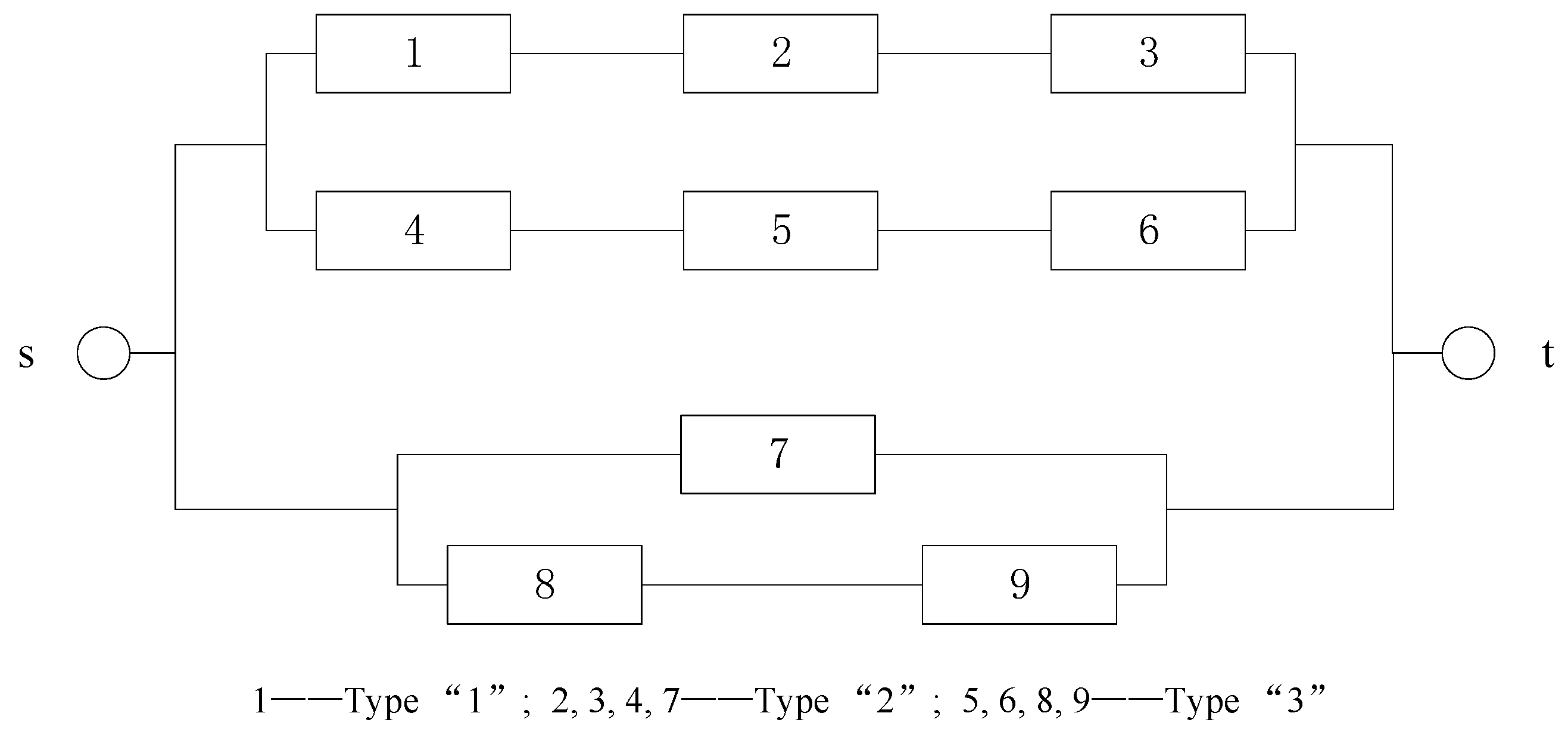
In this section, this study examines the performance of different estimation methods through simulation. It then takes into account a system with nine components, as shown in Figure 2. The system components are grouped into three types, with component “1” being the first type, the second type including components “2, 3, 4, 7”, and the third type including components “5, 6, 8, 9”.

Table A1. Survival signature of the system is presented in Figure 1.

${\mathit{l}}_1$	${\mathit{l}}_2$	${\mathit{l}}_3$	Φ(${\mathit{l}}_1,{\mathit{l}}_2,{\mathit{l}}_3$)	${\mathit{l}}_1$	${\mathit{l}}_2$	${\mathit{l}}_3$	Φ(${\mathit{l}}_1,{\mathit{l}}_2,{\mathit{l}}_3$)
0	0	0	0	1	0	0	0
0	0	1	0	1	0	1	0
0	0	2	1/6	1	0	2	1/3
0	0	3	1/2	1	0	3	1
0	0	4	1	1	0	4	1
0	1	0	1/4	1	1	0	1/4
0	1	1	1/4	1	1	1	3/8
0	1	2	5/12	1	1	2	2/3
0	1	3	3/4	1	1	3	1
0	1	4	1	1	1	4	1
0	2	0	1/2	1	2	0	2/3
0	2	1	7/12	1	2	1	3/4
0	2	2	3/4	1	2	2	8/9
0	2	3	11/12	1	2	3	1
0	2	4	1	1	2	4	1
0	3	0	1	1	3	0	1
0	3	1	1	1	3	1	1
0	3	2	1	1	3	2	1
0	3	3	1	1	3	3	1
0	3	4	1	1	3	4	1
0	4	0	1	1	4	0	1
0	4	1	1	1	4	1	1
0	4	2	1	1	4	2	1
0	4	3	1	1	4	3	1

,

Table A2. Maximum likelihood estimation (MLE) of all parameters and $R_{ss}$.

Types of Components	(${\mathit{\theta }}_{\mathit{k}},{\mathit{\beta }}_{\mathit{k}},{\mathit{\lambda }}_{\mathit{k}}$)	(${\mathit{n}}_{\mathit{k}},{\mathit{m}}_{\mathit{k}}$)	${\widehat{\mathit{\theta }}}_{\mathit{k}}$	${\widehat{\mathit{\beta }}}_{\mathit{k}}$	${\widehat{\mathit{\lambda }}}_{\mathit{k}}$	${\widehat{\mathit{R}}}_{\mathit{s}\mathit{s}}$
1 2 3	(1.2, 2, 0.5) (0.75, 0.5, 1) (1.5, 0.9, 2)	(10, 10)	1.2721	2.1388	0.5249	0.6359
		(40, 40)	0.7647	0.5091	0.9687
		(40, 40)	1.5175	0.9236	2.0072
		(10, 15)	1.2689	2.0711	0.5222	0.6347
		(40, 60)	0.7628	0.5085	1.0627
		(40, 60)	1.5186	0.9071	2.0320
		(15, 10)	1.2376	2.2158	0.5099	0.6289
		(60, 40)	0.7782	0.5077	0.9841
		(60, 40)	1.5228	0.9096	1.9775
		(20, 20)	1.2547	2.0626	0.5251	0.6287
		(80, 80)	0.7635	0.4993	1.0147
		(80, 80)	1.5085	0.8945	2.0053
1 2 3	(1.5, 2, 0.5) (1.2, 0.5, 1) (2, 0.9, 2)	(10, 10)	1.6319	2.1601	0.5363	0.5003
		(40, 40)	1.2163	0.5153	1.0815
		(40, 40)	2.0707	0.8877	1.9999
		(10, 15)	1.5889	2.0870	0.5136	0.5011
		(40, 60)	1.2236	0.5003	1.0080
		(40, 60)	2.0144	0.9070	2.0276
		(15, 10)	1.5847	2.0527	0.5442	0.5055
		(60, 40)	1.2105	0.5214	0.9819
		(60, 40)	2.0182	0.8963	2.0707
		(20, 20)	1.5452	2.0732	0.5036	0.5032
		(80, 80)	1.2078	0.5095	1.0271
		(80, 80)	2.0373	0.9059	2.0248
1 2 3	(1.2, 2.5, 0.5) (0.75, 1, 1) (1.5, 1.5, 2)	(10, 10)	1.2948	2.6886	0.5408	0.8189
		(40, 40)	0.7631	1.0314	1.0261
		(40, 40)	1.5335	1.5183	1.9573
		(10, 15)	1.2869	2.5998	0.5360	0.8197
		(40, 60)	0.7575	1.0229	1.0052
		(40, 60)	1.5203	1.5093	2.0379
		(15, 10)	1.2762	2.6776	0.5232	0.8198
		(60, 40)	0.7569	1.008	1.0058
		(60, 40)	1.5091	1.5564	2.0132
		(20, 20)	1.2718	2.5441	0.5017	0.8180
		(80, 80)	0.7515	1.0153	0.9859
		(80, 80)	1.5335	1.4997	2.0014

,

Table A3. The average relative error of all parameters and $R_{ss}$ for MLE.

Types of Components	(${\mathit{\theta }}_{\mathit{k}},{\mathit{\beta }}_{\mathit{k}},{\mathit{\lambda }}_{\mathit{k}}$)	(${\mathit{n}}_{\mathit{k}},{\mathit{m}}_{\mathit{k}}$)	${\widehat{\mathit{\theta }}}_{\mathit{k}}$	${\widehat{\mathit{\beta }}}_{\mathit{k}}$	${\widehat{\mathit{\lambda }}}_{\mathit{k}}$	${\widehat{\mathit{R}}}_{\mathit{s}\mathit{s}}$
1 2 3	(1.2, 2, 0.5) (0.75, 0.5, 1) (1.5, 0.9, 2)	(10, 10)	0.0601	0.0694	0.0498	0.0033
		(40, 40)	0.0196	0.0181	0.0313
		(40, 40)	0.0117	0.0262	0.0036
		(10, 15)	0.0574	0.0356	0.0445	0.0015
		(40, 60)	0.0171	0.0170	0.0627
		(40, 60)	0.0124	0.0079	0.0160
		(15, 10)	0.0313	0.1079	0.0198	0.0077
		(60, 40)	0.0376	0.0154	0.0159
		(60, 40)	0.0152	0.0107	0.0112
		(20, 20)	0.0455	0.0313	0.0501	0.0079
		(80, 80)	0.0180	0.0013	0.0147
		(80, 80)	0.0057	0.0061	0.0026
1 2 3	(1.5, 2, 0.5) (1.2, 0.5, 1) (2, 0.9, 2)	(10, 10)	0.0879	0.0801	0.0727	0.0020
		(40, 40)	0.0136	0.0306	0.0815
		(40, 40)	0.0353	0.0136	0.0001
		(10, 15)	0.0593	0.0435	0.0272	0.0005
		(40, 60)	0.0196	0.0005	0.0080
		(40, 60)	0.0072	0.0077	0.0138
		(15, 10)	0.0565	0.0264	0.0885	0.0084
		(60, 40)	0.0087	0.0428	0.0181
		(60, 40)	0.0091	0.0041	0.0353
		(20, 20)	0.0302	0.0366	0.0072	0.0036
		(80, 80)	0.0065	0.0190	0.0271
		(80, 80)	0.0187	0.0065	0.0124
1 2 3	(1.2, 2.5, 0.5) (0.75, 1, 1) (1.5, 1.5, 2)	(10, 10)	0.0790	0.0754	0.0817	0.0004
		(40, 40)	0.0175	0.0314	0.0261
		(40, 40)	0.0223	0.0122	0.0213
		(10, 15)	0.0724	0.0399	0.0720	0.0009
		(40, 60)	0.0099	0.0229	0.0052
		(40, 60)	0.0135	0.0062	0.0190
		(15, 10)	0.0635	0.0711	0.0464	0.0010
		(60, 40)	0.0092	0.0080	0.0058
		(60, 40)	0.0060	0.0376	0.0066
		(20, 20)	0.0599	0.0177	0.0034	0.0012
		(80, 80)	0.0020	0.0153	0.0141
		(80, 80)	0.0223	0.0002	0.0007

,

Table A4. Bootstrap-p confidence interval of stress–strength reliability.

Types of Components	(${\mathit{\theta }}_{\mathit{k}},{\mathit{\beta }}_{\mathit{k}},{\mathit{\lambda }}_{\mathit{k}}$)	(${\mathit{n}}_{\mathit{k}},{\mathit{m}}_{\mathit{k}}$)	L-Conf	U-Conf	Length	Coverage
1 2 3	(1.2, 2, 0.5) (0.75, 0.5, 1) (1.5, 0.9, 2)	(10, 10)	0.5446	0.9947	0.4501	0.8782
		(40, 40)
		(40, 40)
		(10, 15)	0.2112	0.7168	0.5056	0.9393
		(40, 60)
		(40, 60)
		(15, 10)	0.5572	0.9971	0.4399	0.8873
		(60, 40)
		(60, 40)
		(20, 20)	0.3536	0.7784	0.4248	0.9558
		(80, 80)
		(80, 80)
1 2 3	(1.5, 2, 0.5) (1.2, 0.5, 1) (2, 0.9, 2)	(10, 10)	0.2706	0.5681	0.2975	0.9055
		(40, 40)
		(40, 40)
		(10, 15)	0.0893	0.7534	0.6641	0.9244
		(40, 60)
		(40, 60)
		(15, 10)	0.4387	0.8604	0.4271	0.8508
		(60, 40)
		(60, 40)
		(20, 20)	0.4874	0.9038	0.4164	0.9252
		(80, 80)
		(80, 80)
1 2 3	(1.2, 2.5, 0.5) (0.75, 1, 1) (1.5, 1.5, 2)	(10, 10)	0.4071	0.9404	0.4414	0.8544
		(40, 40)
		(40, 40)
		(10, 15)	0.4116	0.9726	0.4737	0.8649
		(40, 60)
		(40, 60)
		(15, 10)	0.6712	0.9995	0.5005	0.8623
		(60, 40)
		(60, 40)
		(20, 20)	0.6755	0.9163	0.4174	0.9476
		(80, 80)
		(80, 80)

,

Table A5. Maximum spacing estimation (MSPE) of all parameters and $R_{ss}$.

Types of Components	(${\mathit{\theta }}_{\mathit{k}},{\mathit{\beta }}_{\mathit{k}},{\mathit{\lambda }}_{\mathit{k}}$)	(${\mathit{n}}_{\mathit{k}},{\mathit{m}}_{\mathit{k}}$)	${\tilde{\mathit{\theta }}}_{\mathit{k}}$	${\tilde{\mathit{\beta }}}_{\mathit{k}}$	${\tilde{\mathit{\lambda }}}_{\mathit{k}}$	${\tilde{\mathit{R}}}_{\mathit{s}\mathit{s}}$
1 2 3	(1.2, 2, 0.5) (0.75, 0.5, 1) (1.5, 0.9, 2)	(10, 10)	2.0360	3.4067	0.4812	0.6364
		(40, 40)	0.8404	0.5691	0.9537
		(40, 40)	2.0277	1.1628	1.8141
		(10, 15)	2.0548	3.0850	0.4743	0.6249
		(40, 60)	0.8832	0.5732	0.9816
		(40, 60)	1.9197	1.0654	1.8572
		(15, 10)	1.6725	3.0420	0.5534	0.6373
		(60, 40)	0.8654	0.5734	0.9405
		(60, 40)	1.9243	1.1648	1.7507
		(20, 20)	1.7887	2.9121	0.4568	0.6314
		(80, 80)	0.8426	0.5455	0.9290
		(80, 80)	1.7249	1.0407	1.8139
1 2 3	(1.5, 2, 0.5) (1.2, 0.5, 1) (2, 0.9, 2)	(10, 10)	2.5646	3.3714	0.4954	0.4971
		(40, 40)	1.5180	0.6003	0.9658
		(40, 40)	2.8684	1.2140	1.6765
		(10, 15)	2.4399	3.0175	0.4691	0.4945
		(40, 60)	1.4019	0.5583	0.9776
		(40, 60)	2.6293	1.1215	1.7523
		(15, 10)	2.2520	3.5240	0.4038	0.5029
		(60, 40)	1.4179	0.5677	0.9671
		(60, 40)	2.6510	1.1951	1.7148
		(20, 20)	2.0697	2.8023	0.4663	0.4936
		(80, 80)	1.3917	0.5576	0.9183
		(80, 80)	2.4926	1.0582	1.7751
1 2 3	(1.2, 2.5, 0.5) (0.75, 1, 1) (1.5, 1.5, 2)	(10, 10)	1.9334	3.8509	0.4782	0.8276
		(40, 40)	0.8990	1.2926	0.9530
		(40, 40)	2.2614	2.3124	1.6543
		(10, 15)	2.0248	3.6945	0.4594	0.8115
		(40, 60)	0.9286	1.2383	0.8747
		(40, 60)	2.0393	1.9183	1.8623
		(15, 10)	1.7778	3.8335	0.4901	0.8309
		(60, 40)	0.8717	1.2337	0.9373
		(60, 40)	2.0931	2.2157	1.6437
		(20, 20)	1.6739	3.6473	0.4462	0.8210
		(80, 80)	0.8455	1.1239	0.9268
		(80, 80)	1.7768	1.8505	1.8142

,

Table A6. The average relative error of all parameters and $R_{ss}$ for MSPE.

Types of Components	(${\mathit{\theta }}_{\mathit{k}},{\mathit{\beta }}_{\mathit{k}},{\mathit{\lambda }}_{\mathit{k}}$)	(${\mathit{n}}_{\mathit{k}},{\mathit{m}}_{\mathit{k}}$)	${\tilde{\mathit{\theta }}}_{\mathit{k}}$	${\tilde{\mathit{\beta }}}_{\mathit{k}}$	${\tilde{\mathit{\lambda }}}_{\mathit{k}}$	${\tilde{\mathit{R}}}_{\mathit{s}\mathit{s}}$
1 2 3	(1.2, 2, 0.5) (0.75, 0.5, 1) (1.5, 0.9, 2)	(10, 10)	0.6966	0.7034	0.0377	0.0041
		(40, 40)	0.1206	0.1381	0.0463
		(40, 40)	0.3518	0.2920	0.0929
		(10, 15)	0.7123	0.5425	0.0514	0.0140
		(40, 60)	0.1777	0.1463	0.0184
		(40, 60)	0.2798	0.1838	0.0714
		(15, 10)	0.3937	0.5210	0.1068	0.0056
		(60, 40)	0.1539	0.1469	0.0595
		(60, 40)	0.2828	0.2942	0.1246
		(20, 20)	0.4906	0.4561	0.0865	0.0037
		(80, 80)	0.1234	0.0911	0.0710
		(80, 80)	0.1499	0.1563	0.0930
1 2 3	(1.5, 2, 0.5) (1.2, 0.5, 1) (2, 0.9, 2)	(10, 10)	0.7097	0.6857	0.0092	0.0085
		(40, 40)	0.2650	0.2006	0.0342
		(40, 40)	0.4342	0.3488	0.1618
		(10, 15)	0.6266	0.5087	0.0618	0.0137
		(40, 60)	0.1682	0.1167	0.0224
		(40, 60)	0.3146	0.2461	0.1238
		(15, 10)	0.5013	0.7620	0.1925	0.0032
		(60, 40)	0.1816	0.1353	0.0329
		(60, 40)	0.3255	0.3279	0.1426
		(20, 20)	0.3798	0.4011	0.0673	0.0154
		(80, 80)	0.1597	0.1152	0.0817
		(80, 80)	0.2463	0.1758	0.1125
1 2 3	(1.2, 2.5, 0.5) (0.75, 1, 1) (1.5, 1.5, 2)	(10, 10)	0.6112	0.5403	0.0436	0.0105
		(40, 40)	0.1987	0.2926	0.0470
		(40, 40)	0.5076	0.5416	0.1728
		(10, 15)	0.6873	0.4778	0.0813	0.0092
		(40, 60)	0.2381	0.2383	0.1253
		(40, 60)	0.3595	0.2789	0.0689
		(15, 10)	0.4815	0.5334	0.0199	0.0145
		(60, 40)	0.1623	0.2337	0.0627
		(60, 40)	0.3954	0.4771	0.1782
		(20, 20)	0.3949	0.4589	0.1076	0.0025
		(80, 80)	0.1273	0.1239	0.0732
		(80, 80)	0.1846	0.2337	0.0929

,

Table A7. Error of the nonlinear system of equations estimated by MSPE.

Types of Components	(${\mathit{\theta }}_{\mathit{k}},{\mathit{\beta }}_{\mathit{k}},{\mathit{\lambda }}_{\mathit{k}}$)	(${\mathit{n}}_{\mathit{k}},{\mathit{m}}_{\mathit{k}}$)	${\tilde{\mathit{\theta }}}_{\mathit{k}}$	${\tilde{\mathit{\beta }}}_{\mathit{k}}$	${\tilde{\mathit{\lambda }}}_{\mathit{k}}$
1 2 3	(1.2, 2, 0.5) (0.75, 0.5, 1) (1.5, 0.9, 2)	(10, 10)	−0.042474	−0.078425	−0.006317
		(40, 40)	0.000014	0.000261	0.001113
		(40, 40)	−0.002183	−0.000760	0.003488
		(10, 15)	−0.046259	−0.074859	−0.005684
		(40, 60)	0.000374	0.000528	0.001972
		(40, 60)	−0.000355	−0.000023	0.001410
		(15, 10)	−0.035156	−0.070763	−0.005434
		(60, 40)	−0.000102	0.000159	0.000835
		(60, 40)	−0.003344	−0.001286	−0.000274
		(20, 20)	−0.039287	−0.086593	−0.007940
		(80, 80)	0.000553	0.000724	0.001947
		(80, 80)	−0.000072	0.000030	0.000446
1 2 3	(1.5, 2, 0.5) (1.2, 0.5, 1) (2, 0.9, 2)	(10, 10)	−0.053372	−0.075868	−0.011874
		(40, 40)	−0.008546	−0.001042	0.000029
		(40, 40)	−0.021196	−0.005235	−0.003993
		(10, 15)	−0.059393	−0.072226	−0.014142
		(40, 60)	0.000208	0.000390	0.001853
		(40, 60)	−0.009048	−0.001696	−0.001304
		(15, 10)	−0.061220	−0.104871	−0.008531
		(60, 40)	−0.002658	−0.000322	0.000291
		(60, 40)	−0.014781	−0.005201	−0.002194
		(20, 20)	−0.071250	−0.101527	−0.009600
		(80, 80)	−0.000010	0.000470	0.001337
		(80, 80)	−0.005522	−0.001175	−0.000398
1 2 3	(1.2, 2.5, 0.5) (0.75, 1, 1) (1.5, 1.5, 2)	(10, 10)	−0.027922	−0.077045	−0.005986
		(40, 40)	−0.003560	−0.008062	−0.001128
		(40, 40)	−0.013136	−0.012954	−0.001938
		(10, 15)	−0.034050	−0.079039	−0.007013
		(40, 60)	−0.002816	−0.006225	−0.001586
		(40, 60)	−0.006415	−0.006044	−0.000842
		(15, 10)	−0.034207	−0.088551	−0.007658
		(60, 40)	−0.000876	−0.001924	−0.000178
		(60, 40)	−0.010053	−0.009830	−0.001762
		(20, 20)	−0.048707	−0.122047	−0.008859
		(80, 80)	−0.000544	−0.001219	−0.000127
		(80, 80)	−0.002637	−0.003949	−0.000484

and

Table A8. Bayes estimation of $R_{ss}$ and 95% HPD intervals.

Types of Components	(${\mathit{\theta }}_{\mathit{k}},{\mathit{\beta }}_{\mathit{k}},{\mathit{\lambda }}_{\mathit{k}}$)	(${\mathit{n}}_{\mathit{k}},{\mathit{m}}_{\mathit{k}}$)	${\widehat{\mathit{R}}}_{\mathit{s}\mathit{s}}^{\mathit{B}}$	${\widehat{\mathit{R}}}_{\mathit{s}\mathit{s}}^{\mathit{B}}$		HPD
				Bias	ARE	L-Conf	U-Conf
1 2 3	(1.2, 2, 0.5) (0.75, 0.5, 1) (1.5, 0.9, 2)	(10, 10)	0.6731	0.0393	0.0982	0.5722	0.7726
		(40, 40)
		(40, 40)
		(10, 15)	0.6770	0.0432	0.0724	0.5844	0.7676
		(40, 60)
		(40, 60)
		(15, 10)	0.6774	0.0436	0.0733	0.5851	0.7685
		(60, 40)
		(60, 40)
		(20, 20)	0.6820	0.0482	0.0671	0.6091	0.7538
		(80, 80)
		(80, 80)
1 2 3	(1.5, 2, 0.5) (1.2, 0.5, 1) (2, 0.9, 2)	(10, 10)	0.6086	0.1073	0.1147	0.5032	0.7122
		(40, 40)
		(40, 40)
		(10, 15)	0.6118	0.1105	0.0966	0.5156	0.7086
		(40, 60)
		(40, 60)
		(15, 10)	0.6140	0.1127	0.0988	0.5160	0.7112
		(60, 40)
		(60, 40)
		(20, 20)	0.6135	0.1122	0.0835	0.5350	0.6922
		(80, 80)
		(80, 80)
1 2 3	(1.2, 2.5, 0.5) (0.75, 1, 1) (1.5, 1.5, 2)	(10, 10)	0.7870	−0.0320	0.0634	0.6993	0.8694
		(40, 40)
		(40, 40)
		(10, 15)	0.7844	−0.0346	0.0554	0.7047	0.8609
		(40, 60)
		(40, 60)
		(15, 10)	0.7842	−0.0348	0.0572	0.7034	0.8610
		(60, 40)
		(60, 40)
		(20, 20)	0.7805	−0.0385	0.0419	0.7175	0.8415
		(80, 80)
		(80, 80)

are all long tables and are presented in the Appendix A.

The calculation of the system survival signature is implemented using the ReliabilityTheory package in R language. Table A1 represents the survival signature of the system in Figure 2. For example, when the first type of component fails (i.e., “1” fails), one out of the second type of components (“2, 3, 4, 7”) are operational, and three out of the third type of components (“5, 6, 8, 9”) are operational, the survival signature of the system $\Phi \left(l_1,l_2,l_3\right)=\Phi \left(0,\mathrm{1,3}\right)=3/4$.

6.1. Parameters Estimation

Let $u_1,u_2,\dots ,u_{n_k}$ and $v_1,v_2,\dots ,v_{m_k}$ be independent random numbers from $U\left(\mathrm{0,1}\right)$. Given the values of parameters ${\theta }_k$ and ${\beta }_k$, the inverse transform method can be used to generate $n_k$ and $m_k$ random numbers that follow the Lomax distribution (where $k=1, 2, 3$). It is the case that various estimates were calculated under small, medium, and large sample sizes, and the control variable method was used to determine how these estimates change with variations in the parameters ${\theta }_k$ and ${\beta }_k$, or with changes in sample size. The above steps were carried out 100 times to obtain the mean and average relative error of various point estimates.

Therefore, three groups of control experiments were set up to analyze the effects of parameter variations on model estimation. Within each group, four subgroup control experiments were conducted to examine how different values of stress and strength data impact the reliability estimation. Since the stress–strength reliability estimation Formula (6) was independent of ${\lambda }_k$, it was fixed while ${\theta }_k$ and ${\beta }_k$ were allowed to vary in order to investigate their impact on the stress–strength reliability. In the first set of experiments, the parameters for three different types of components were set as follows: $({\theta }_1,{\beta }_1,{\lambda }_1)=(1.2, 2, 0.5)$, $({\theta }_2,{\beta }_2,{\lambda }_2)=(0.75, 0.5, 1)$ and $({\theta }_3,{\beta }_3,{\lambda }_3)=$ $(1.5, 0.9, 2).$ In the second set of experiments, the parameters were adjusted to: $({\theta }_1,{\beta }_1,{\lambda }_1)=(1.5, 2, 0.5), ({\theta }_2,{\beta }_2,{\lambda }_2)=(1.2, 0.5, 1)$ and $({\theta }_3,{\beta }_3,{\lambda }_3)=(2, 0.9, 2)$. The shape parameters ${\beta }_k$ of the stress variables and the common scale parameters ${\lambda }_k$ (for $k=1, 2, 3)$ were kept constant to study the effects of increasing the shape parameters ${\theta }_k$ of the strength variables on the estimation results and errors across different sample sizes. Similarly, in the third set of experiments, the parameters were set as follows: $({\theta }_1,{\beta }_1,{\lambda }_1)=(1.2, 2.5, 0.5),$ $({\theta }_2,{\beta }_2,{\lambda }_2)=(0.75, 1, 1)$ and $({\theta }_3,{\beta }_3,{\lambda }_3)=(1.5, 1.5, 2)$. Compared to the first set of experiments, this set up effectively keeps the shape parameters ${\theta }_k$ of the strength variables and the common scale parameters ${\lambda }_k$ constant, allowing for the study of how increasing the shape parameters ${\beta }_k$ of the stress variables influences the estimation results and errors across various sample sizes.

6.1.1. Maximum Likelihood Estimation and Bootstrap-p Confidence Interval

Table A2 provides the results of the maximum likelihood estimation. The first two sets of experimental data indicate that, when ${\beta }_k$ and ${\lambda }_k$ were held constant, an increase in the parameter ${\theta }_k$ results in a decrease in system reliability. Similarly, the results from the first and third sets of experiments demonstrate that, when ${\theta }_k$ and ${\lambda }_k$ were kept constant, an increase in the parameter ${\beta }_k$ leads to an increase in the system reliability. The change in sample size has a slight impact on the estimation of reliability, and its effect is not very significant. This is reflected in all three sets of experiments in Table A2. For instance, when the sample sizes $(n_1,m_1,n_2,m_2,n_3,m_3)$ increases from $(10, 10, 40, 40, 40, 40)$ to $(20, 20, 80, 80, 80, 80)$, doubling the sample size, the stress–strength reliability of the experiments changes only slightly from $(0.6359, 0.5003, 0.8189)$ to $(0.6287, 0.5032, 0.8180)$. However, this slight variation does not exclude the influence of random simulation errors on the experimental results. Overall, the increase in sample size shows a minor and insignificant effect on system reliability. Furthermore, compared to the first and second sets of experiments, it was evident that when the shape parameters ${\theta }_k$ of the strength variables increase, the estimated reliability of stress–strength decreases. Evidently, this conclusion can also be analyzed and derived from the monotonicity of the function in Equation (6). Similarly, when compared to the first and third sets of experiments, an increase in the shape parameters ${\beta }_k$ of the stress variables leads to an increase in the estimated reliability. However, this conclusion cannot be analyzed or derived based on the monotonicity of the function in Equation (6). The shape parameters of the strength variables and the stress variables play opposite roles in the estimation of reliability, which allows us to more accurately predict and adjust the reliability performance of systems.

The average relative errors of the maximum likelihood estimation are presented in Table A3, calculated using formula $ARE\left({\widehat{\eta }}_k\right)=|{\widehat{\eta }}_k-{\eta }_k|/{\eta }_k$, where ${\eta }_k={\theta }_k, {\beta }_k, {\lambda }_k$ and $R_{ss}$, while ${\widehat{\eta }}_k$ represents the estimate values of ${\theta }_k, {\beta }_k, {\lambda }_k$ and $R_{ss}$. Analyzing the data presented in Table A3, it is evident that, with exceptions for certain data points that are impacted by random simulations, the average relative error for most parameters tends to decrease as the sample size increases. Moreover, by ignoring the individual effects of random simulations, it is clear that with a fixed sample size, increasing the shape parameters of either the strength variables or the stress variables lead to a reduction in the relative error of reliability estimates. Notably, increasing the shape parameters of the stress variables significantly reduces the relative error, often bringing it to a very low level.

Subsequently, the 95% Bootstrap confidence intervals were calculated based on the maximum likelihood estimates of each parameter. Table A4 shows the average confidence intervals obtained by running Algorithm 2 for 1000 iterations, and based on these, the average length of the confidence intervals and the average coverage rate were calculated. The experimental results indicate that the Bootstrap method achieves a high coverage rate, all exceeding 85%.

6.1.2. Maximum Spacing Estimation in Point Estimation

Table A5, Table A6 and Table A7 present the results of the maximum spacing estimation for all parameters and the stress strength reliability $R_{ss}$. During the calculation process, the L-BFGS-B algorithm was employed to solve the nonlinear system of Equation (15). The objective function was set as the sum of the squares of the partial derivatives, and the goal was to minimize this function to find the roots of the system of equations. In the optimization process, the lower bounds for the parameters ${\theta }_k$, ${\beta }_k$, and ${\lambda }_k$ were all set to 0.01, and the upper bounds were set to 5. Through iterative loops, the MSPE for all parameters and ${\tilde{R}}_{ss}$ were obtained and shown in Table A5, the mean relative error in Table A6, and the iterative error of the system of equations in Table A7.

From Table A5, it can be seen that, apart from the uncertainties brought by individual random simulations, the estimation results of most parameters achieve closer to the true values as the sample size increases. The same conclusion can also be drawn from Table A6, which shows that the relative estimation error of parameters decreases as the sample size increases. Furthermore, from the three sets of experiments in Table A5 and Table A6, we can observe that when the sample size $(n_1,m_1,n_2,$ $m_2,n_3,m_3)$ increases from $(10, 10, 40, 40, 40, 40)$ to $(10, 15, 40, 60, 40, 60)$ or $(15, 10, 60, 40, 60,$ $40)$, whether it is an increase in the sample size of the stress variables or an increase in the sample size of the strength variables, both contribute to reducing the estimation error of the parameters. Furthermore, the stress strength reliability decreases as the shape parameter ${\theta }_k$ of the strength variable increases, and increases as the shape parameter ${\beta }_k$ of the stress variable increases. This conclusion is consistent with the maximum likelihood estimation, and it can also be reached by conducting a monotonicity analysis on Equation (6). Comparing Table A6 with Table A3, it is found that, overall, the average relative error of the maximum likelihood estimation is smaller than that of MSPE. Table A7 presents the verification results obtained by substituting the MSPE values of the parameters from Table A5 into equation set (15). All calculation results are below 0.2, with 96% of them being less than 0.09 and nearly 70% below 0.009. This suggests that the computational outcomes are highly accurate.

6.1.3. Bayesian Estimation and 95% HPD Confidence Interval

Table A8 presents the results of Bayesian estimation, which includes the estimated values of the stress–strength reliability ${\widehat{R}}_{ss}^B$, the bias and average relative error of the Bayesian estimates, and the last two columns provide the lower and upper bounds of the 95% HPD confidence interval.

In Bayesian estimation, parameters $a_{k,i}$ and $b_{k,i}$ of the gamma prior were set to 1, where $k,i=1, 2, 3$. The algorithm was iterated 100 times, and the average values were calculated to obtain the Bayesian average estimate of ${\widehat{R}}_{ss}^B$, along with its bias and average relative error. The experimental results show that the bias in the first and third sets of experiments is relatively small, all below 0.05, while the bias in the second set of experiments is larger, ranging from 0.1 to 0.13. Therefore, it can be concluded that, when holding other parameters constant, the accuracy of Bayesian estimation decreases as the shape parameters ${\theta }_k$ of the strength variables increase. The bias of Bayesian estimation is relatively sensitive to changes in parameters. By comparing these three groups of experiments, it can be found that when ${\theta }_k$ increases, the bias significantly increases, indicating that the estimated values are larger. When ${\beta }_k$ increases, the bias significantly decreases and is entirely negative, indicating that the estimated values are smaller. In addition, the results in Table A8 indicate that, as the sample size increases, the accuracy of Bayesian estimation gradually improves, with average relative error decreasing, and the Highest Posterior Density interval also becoming narrower. Different parameter settings have an impact on the estimation results, but the general trend is that the larger the sample size, the more reliable the estimation results become.

In conclusion, regarding estimation accuracy, the results indicate that ${\widehat{R}}_{ss}^B<{\tilde{R}}_{ss}<{\widehat{R}}_{ss}$. This suggests that the maximum likelihood estimation yields the highest precision, followed by the maximum spacing estimation, and lastly, the Bayesian estimation. This result is due to the combined effects of several factors, including differences in sample size, the choice of prior information, computational complexity, and system structure. In complex systems with diverse system types, when the same prior distribution is applied to different types of components, it will affect the estimation accuracy of the model. However, as the sample size increases, the influence of the prior distribution on the estimation results will become smaller and smaller. It can also be seen from Table A8 that as the sample size increases, the average relative error gradually decreases. Furthermore, Bayesian estimation involves complex calculations, such as MCMC methods, which can converge too slowly with large sample sizes. In contrast, maximum likelihood estimation and maximum spacing estimation do not rely on prior information and perform more stably with larger sample sizes.

6.2. Dynamic Stress–Strength Reliability Estimation

Subsequently, the maximum likelihood estimation results of each parameter were utilized to verify the dynamic stress–strength reliability model proposed in Section 5. For the parameters in models (23) and (25), the MLE results from the first set of experiments in Table A2 were employed to verify the dynamic model which was presented in Section 5, where $\left({\widehat{\theta }}_1,{\widehat{\beta }}_1,{\widehat{\lambda }}_1\right)=(1.2547, 2.0626, 0.5251)$, $\left({\widehat{\theta }}_2,{\widehat{\beta }}_2,{\widehat{\lambda }}_2\right)=\left(0.7635, 0.4993, 1.0147\right)$, and $\left({\widehat{\theta }}_3,{\widehat{\beta }}_3,{\widehat{\lambda }}_3\right)=(1.5085,$ $0.8945,$ 2.0053).

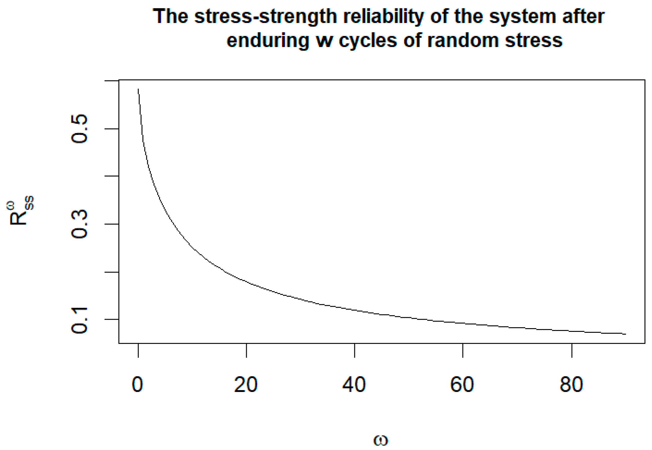
Under the action of cyclic stresses, the unit degradation amounts of the strength variables for different types of components are taken as $({\xi }_1,{\xi }_2,{\xi }_3)=\left(\mathrm{0.1,\; 0.2,\; 0.3}\right)$. The first set of parameters estimated from Table A2 was used for simulation experiments. Then, the first set of parameters was substituted into Equation (23), and Algorithm 4 was applied to estimate the generalized integral in Equation (24). Figure 3 illustrates the reliability varying with cyclic stress, demonstrating that the stress–strength reliability of the system decreases gradually as the number of cycles increases. According to the definition of reliability, when the stress increases, the system reliability will gradually decrease. The experimental results in Figure 3 are consistent with the definition, which indicates that Algorithm 4 is feasible and accurate in the approximate estimation of the stress–strength reliability.

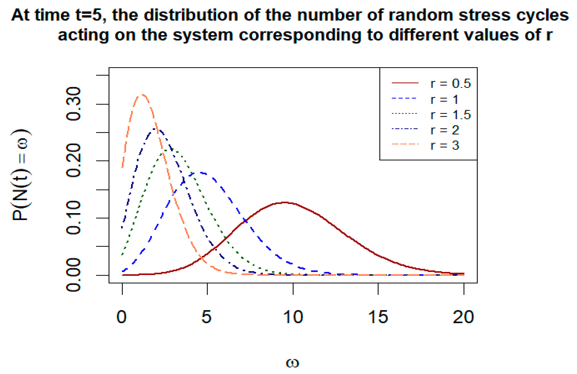
The number of cyclic stresses follows a Poisson distribution with parameter $t/r$. Let $t=5$, and $r$ take the values $0.5, 1, 1.5, 2,$ and $3$. The probability distribution of the number of cycles $\omega$ within the time interval $(0, t]$ is shown in Figure 4. From the results, we can see that as $r$ increases, the probability distribution gradually changes from a symmetric distribution to a right-skewed distribution. The same conclusion can be obtained by analyzing the meaning of Equation (22). When $t$ is fixed and $r$ increases, the probability of $\omega$ stress cycles occurring within the time period $(0,t]$ will also decrease accordingly. $t/r$ is equivalent to reducing the length of the time interval. The larger $r$ is, the smaller the time interval $(0,t/r]$ will be. Obviously, there will not be too many cyclic stresses within a smaller time period.

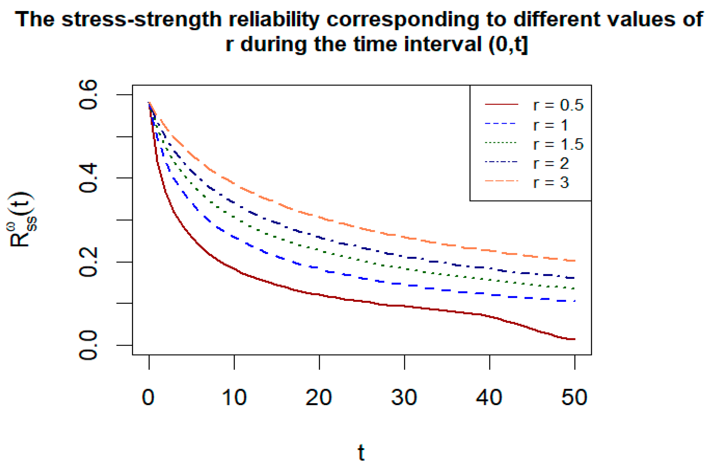
Figure 5 shows the dynamic stress–strength reliability of the system over the time interval $(0, t]$. For different values of $r$, specifically $r=0.5, 1, 1.5, 2$ and $3$, the reliability values were approximately calculated using Algorithm 4. From the figure, it can be observed that the larger the value of $r$, the more slowly the system reliability decays over time. The conclusions of Figure 4 and Figure 5 are consistent. The larger the value of $r$, the shorter the transformed time interval $(0,t/r]$ is. Therefore, the probability of $\omega$ stress cycles occurring is also smaller. In the stress–strength reliability model, at the same moment, when the strength is fixed, the smaller the stress, the higher the reliability. In addition, when $t=0$, the result of the dynamic reliability model (25) becomes that of the static model. The estimated value approximately obtained according to Algorithm 4 is 0.5823. Compared with the estimated result of 0.6287 in Table A2, the error is 0.0464. The error is relatively small, indicating that the result is fairly accurate.

Through the above simulation experiments, the problem of system reliability estimation under periodic stress was solved. From Figure 3 and Figure 5, it can be seen that whether the number of stress cycles increases or the time interval increases, the system reliability gradually decreases, which is also the principle of the reliability model.

6.3. Sensitivity Analysis

6.3.1. Sensitivity Analysis of Stress–Strength Reliability to the Parameters of the Lomax Distribution

Next, from a quantitative analysis perspective, the extent to which the stress–strength reliability estimates are affected when parameters $({\theta }_1,{\theta }_2,{\theta }_3)$ and $({\beta }_1,{\beta }_2,{\beta }_3)$ undergo sequential changes under the three parameter estimation methods will be systematically examined. Through this process, the underlying patterns regarding how the variations in these parameters impact the reliability estimation results are aimed to be uncovered. The parameters were set as follows: $({\theta }_1,{\beta }_1,{\lambda }_1)=(1.2,2.5,0.5),$ $({\theta }_2,{\beta }_2,{\lambda }_2)=(0.75,1,1)$, and $({\theta }_3,{\beta }_3,{\lambda }_3)=(1.5,1.5,2)$. The model in Equation (6) is independent of the parameter ${\lambda }_k$, so the sensitivity of ${\lambda }_k$ is unnecessary. In each group of experiments, all other parameters were held constant. The fluctuations in the system stress–strength reliability were analyzed successively as parameters ${\theta }_1,{ \theta }_2, {\theta }_3$, ${\beta }_1,{ \beta }_2$, and ${\beta }_3$ were adjusted individually. 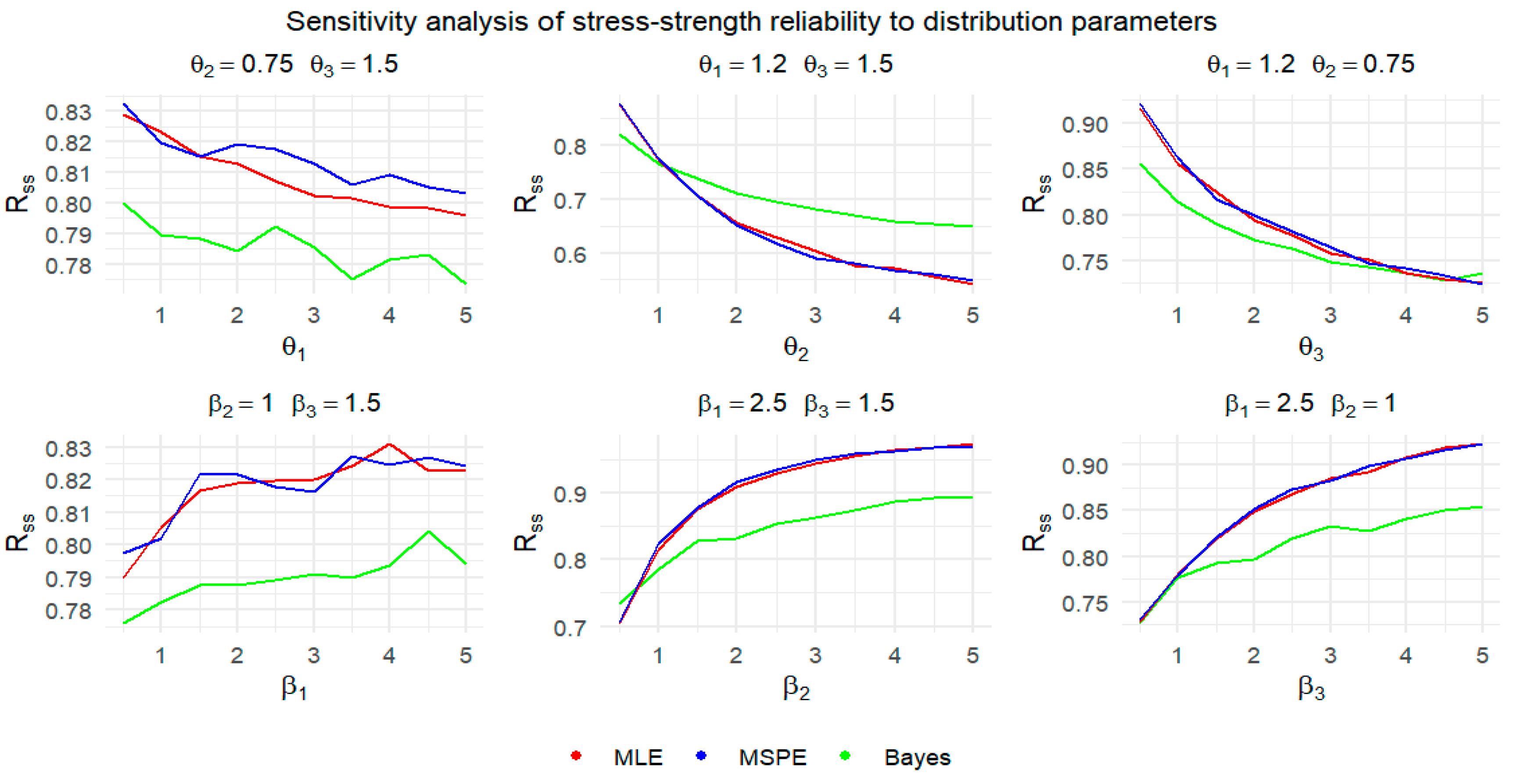Figure 6 depicts the shifts in reliability when the aforementioned six parameters are tweaked successively under three different estimation methods.

From the commonalities of the above six sub-figures in Figure 6, the larger the shape parameter ${\theta }_k(k=1, 2, 3)$ of the strength variable, the lower the reliability. The larger the shape parameter ${\beta }_k(k=1, 2, 3)$ of the stress variable, the higher the reliability. Numerically, the changes in parameters ${\theta }_1$ and ${\beta }_1$ have the least impact on the estimated reliability value. When ${\theta }_1$, ${\theta }_2$ and ${\theta }_3$ (or ${\beta }_1$, ${\beta }_2$, and ${\beta }_3$) change from 0.5 to 5, the ranges of change in reliability are approximately 0.027–0.041, 0.159–0.334, and 0.127–0.197, respectively. The existence of redundant design in the system may lead to a smaller impact of changes in parameters ${\theta }_1$ and ${\beta }_1$ on reliability. Obviously, when Type 1 only contains component “1”, the normal operation of this component does not have a significant impact on the system reliability. However, whether the components in Type 2 and Type 3 are faulty and the number of faulty components will significantly affect the reliability estimation. This also results in the stress–strength reliability being relatively significantly affected by the changes in these parameters such as ${\theta }_2$, ${\beta }_2$, ${\theta }_3$, and ${\beta }_3$. From the perspective of parameter estimation methods, Figure 6 shows that the results of MLE and MSPE are very close, while the results of the Bayesian estimation differ significantly from those of the above two estimation methods under certain circumstances. As these parameters increase, the results of the Bayesian estimation begin to diverge from those of the other two methods. Overall, the trend indicates that the variation range of the Bayesian estimation is relatively smoother compared to the other two methods. This is because the MLE is highly sensitive to the distribution assumptions of the data, while the MSPE is very sensitive to extreme values in the data. The results of these two parameter estimation methods can fluctuate significantly due to changes in the data distribution. The introduction of prior information can smooth out the changes in parameter estimation. Therefore, Bayesian estimation may exhibit lower sensitivity when parameters change.

6.3.2. Sensitivity Analysis of Stress–Strength Reliability to Sample Size

In addition, in Section 6.1, the estimation errors of the model were analyzed by setting the sample sizes of the stress and strength variables of each type of component as (10, 10, 40, 40, 40, 40), (10, 15, 40, 60, 40, 60), (15, 10, 60, 40, 60, 40), and (20, 20, 80, 80, 80, 80), respectively. The preliminary analysis results show that MLE and MSPE are not very sensitive to the changes in sample size, though there is also a certain degree of reduction. In contrast, the estimation error of Bayesian estimation decreases significantly as the sample size increases. However, the values of these sample sizes are not comprehensive enough. Next, the sample size will be considered as an uncertain factor, and the impacts of its different values on the estimation results of the stress–strength reliability model will be analyzed in detail. The parameters of Lomax distribution were set as follows: $({\theta }_1,{\beta }_1,{\lambda }_1)=(1.2,2.5,0.5),$ $({\theta }_2,{\beta }_2,{\lambda }_2)=(0.75,1,1)$, and $({\theta }_3,{\beta }_3,{\lambda }_3)=(1.5,\mathrm{1.5,2})$.

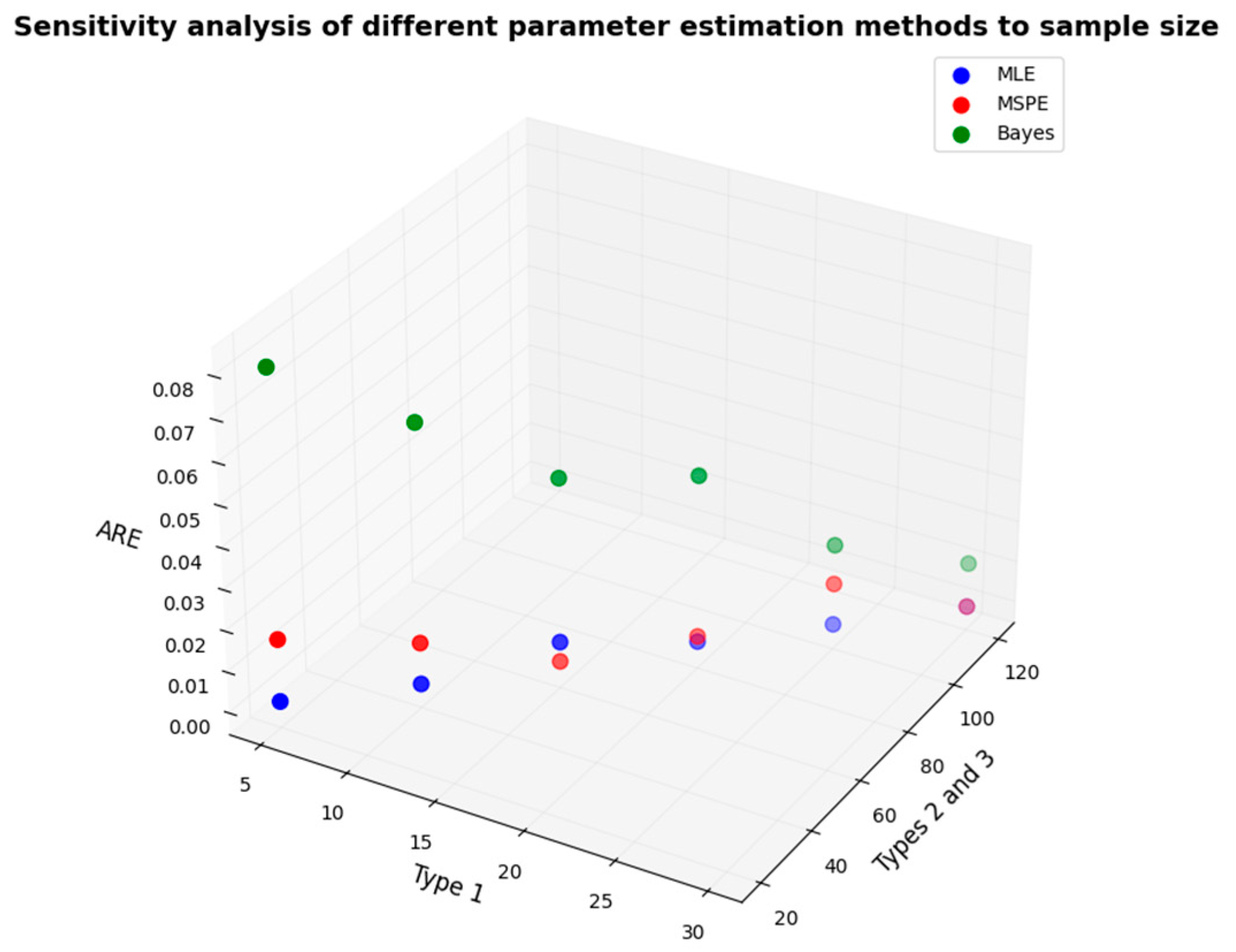
In the following, the changes in the average relative error of the stress–strength reliability model will be analyzed when the sample sizes of stress and strength variables change from (5, 5, 20, 20, 20, 20) to (30, 30, 120, 120, 120, 120), respectively. In the system shown in Figure 2, the number of components of types “2” and “3” is four times that of type “1”. Therefore, during the process of sample size analysis, the sample sizes of types “2” and “3” are also set to be four times that of type “1”. Figure 7 shows the results of the sensitivity analysis of the estimation errors of the stress–strength model to the sample size under three estimation methods. It can be seen from Figure 7 that as the sample size increases, the average relative errors of these three estimation methods all decrease. Among them, the error of MLE is the smallest, followed by that of MSPE. The accuracy of these two estimation methods has already shown excellent performance in the case of small sample sizes. However, the Bayesian estimation is affected by the prior distribution when the sample size is small, and its error is larger compared with the first two estimation methods. But as the sample size increases, the error gradually decreases, and it shows good estimation accuracy in the case of large sample sizes.

6.3.3. Sensitivity Analysis of the Dynamic Stress–Strength Model to the Hyperparameters of Variable Degradation

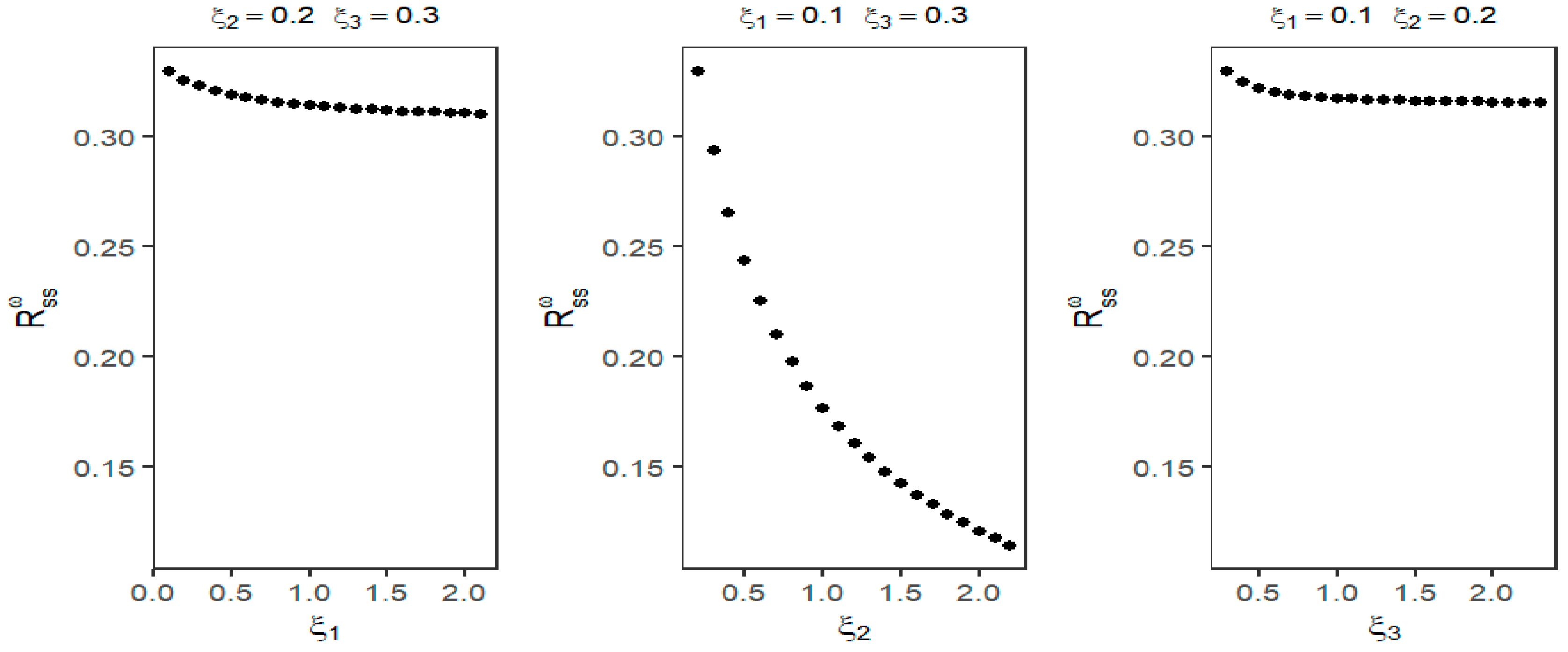
In the following, the impact of changes in the individual degradation amounts ${\xi }_1, {\xi }_2$ and ${\xi }_3$ of the strength variables of different types of components on the stress–strength reliability under cyclic stress will be analyzed.

In each experimental group, the system undergoes five cycles of stress application. Then, through the method of controlled variables, the variations in stress–strength reliability with respect to ${\xi }_1, {\xi }_2$ and ${\xi }_3$ were analyzed. The parameter estimation results of the MLE are used, and the results corresponding to the fourth sample size in the first set of experiments in Table A2 are selected for analysis. The parameters were set as follows:$\left({\widehat{\theta }}_1,{\widehat{\beta }}_1,{\widehat{\lambda }}_1\right)=\left(1.2547, 2.0626, 0.5251\right)$, (${\widehat{\theta }}_2,{\widehat{\beta }}_2,{\widehat{\lambda }}_2)=\left(0.7635, 0.4993, 1.0147\right)$, and $\left({\widehat{\theta }}_3,{\widehat{\beta }}_3,{\widehat{\lambda }}_3\right)=(\mathrm{1.5085,0.8945}, 2.0053)$. The findings are illustrated in Figure 8.

From Figure 8, it can be seen that as ${\xi }_1, {\xi }_2$, and ${\xi }_3$ increase, the reliability gradually decreases. Apparently, this conclusion is easy to explain. Obviously, when the unit degradation amounts of the strength variables increase, the probability that the strength exceeds the stress under the same stress decreases, leading to a lower system reliability. The change of ${\xi }_2$ has the most significant impact on the reliability. The impacts of the changes of ${\xi }_1$ and ${\xi }_3$ on the reliability are less significant than those of ${\xi }_2$. The reason for this result is still related to the system structure in Figure 2. ${\xi }_2$ is the unit degradation amount of the strength variable corresponding to component type “2”. From the perspective of the importance of different types of components, components of type “2” have the most significant impact on the change in the system reliability.

7. Conclusions

This paper mainly solves two core problems. One is that for systems where both stress and strength variables follow the Lomax distribution, it extends the traditional stress–strength reliability model, which is usually applied to single-component types or systems with relatively simple structures, to complex multi-component systems, so as to enrich the research on reliability theory. The other is to introduce the time variable into the traditional static stress–strength model and expand it into a dynamic stress–strength model that is more suitable for practical needs.

Regarding the first question, let the strength and stress variables of each type of component follow the Lomax distribution. Assuming that the scale parameters ${\lambda }_k$ of the strength and stress variables are identical, the stress–strength reliability model is derived based on survival signature theory. Next, various point estimates were formulated, including the MLE, the MSPE, and the Bayesian estimate, for the parameters and the reliability model. Additionally, the 95% Bootstrap-p confidence interval for the MLE and the HPD confidence interval for the Bayesian estimate using the MCMC algorithm were provided. Finally, a numerical experiment on a system consisting of nine components across three different types was performed and the average relative error of various estimation methods was calculated. Finally, the sensitivities of the three estimation methods to parameter changes and sample size, as well as the sensitivity of the dynamic stress–strength model to the unit degradation amount of strength variables, were discussed, respectively. Moreover, the reasons behind these results were analyzed from the perspectives of system structure and estimation methods. The results show that MLE has the highest estimation accuracy, followed by MSPE. Moreover, these two estimation methods can achieve relatively high estimation accuracy even with a small sample size. For example, when the sample sizes are set as (5, 5, 20, 20, 20, 20), the average relative error of MLE is only 0.1%, that of MSPE is 1.62%, while the error of Bayesian estimation is 8.05%. The accuracy of Bayesian estimation is lower than that of the previous two methods. On the one hand, when the sample size is small, Bayesian estimation is easily affected by the prior distribution. On the other hand, Bayesian estimation requires calculating the posterior distribution, and in many practical problems, the form of the posterior distribution can be very complex. For instance, it is quite difficult to calculate Equation (17) in this paper accurately. Usually, numerical methods are needed to obtain approximate solutions. For example, Algorithm 1 uses the Markov Chain Monte Carlo method for solving. These methods will introduce calculation errors, and the convergence and stability of the calculation process will also affect the estimation accuracy. In contrast, MLE usually only needs to find the maximum value of the likelihood function, and MSPE determines the classification boundary by optimizing a convex function. Its calculation process is relatively simple and straightforward, and is less affected by calculation errors. As the sample size increases, the average relative error of Bayesian estimation gradually decreases. When the sample size is (30, 30, 120, 120, 120, 120), the average relative error of the model drops to 1.12%. Therefore, in a large-sample environment, for the stress–strength model, Bayesian estimation is still a good estimation method.

Regarding the second question, the Poisson process is used to describe the degradation process of the stress variables over time. The change process of the strength variables over time is achieved by introducing hyperparameters ${\xi }_k$, where $k=1, 2, 3$, which are used to describe the unit degradation amount of the strength variables under the action of periodic stress, thus also associating them with the time variable. By applying different periodic random stresses to various types of components, the dynamic stress–strength reliability model of the system that changes over time is derived, and an approximate calculation algorithm for this model is provided through Algorithm 4. In addition, the feasibility and accuracy of the dynamic stress–strength reliability model are verified through this system, thus solving Problem 2. Substitute a set of results from the MLE into the dynamic stress–strength reliability model. By comparing it with the static model at the moment of $t=0$, the estimated error is 0.0464, which is relatively small. Therefore, the model has a relatively high accuracy rate. In the sensitivity analysis, affected by the system structure, the parameters corresponding to different types of components have different impacts on the stress–strength reliability. Influenced by the system redundancy design and the importance of each type of component in the system, changes in each parameter among the stress variable, strength variable, and the unit degradation amount of the strength variable of type “1” components have the least impact on the reliability. Changes in these parameters of type “2” and “3” components have the greatest impact on the reliability. The estimation results of the three estimation methods, MLE and MSPE, are similar. Bayesian estimation is not as sensitive to parameter changes as the first two estimation methods.

In future research, the following aspects can be considered. First, regarding the assumptions for model simplification, this paper assumes that stress variables and strength variables are independent of each other. In real life, there may be certain dependence relationships among many stress factors such as temperature, pressure, and friction, or strength factors like high-temperature resistance, pressure resistance, and wear resistance. Therefore, relevant theories such as the copula function can be used to analyze the correlations between these variables. Second, models corresponding to various types of censored data can be considered, such as Type-I censoring, Type-II censoring, progressive Type-I censoring, or progressive Type-II censoring. Stress–strength models can be established from the perspective of complex data types. In addition, in this paper, the model was simplified by assuming that the stress and strength variables within the same type of component have the same scale parameter. Therefore, the estimation of reliability models can be studied when the scale parameters of stress and strength variables are different. Apart from the above aspects, the application of the dynamic stress–strength model proposed in Section 5 in the field of system maintenance can be explored. Moreover, a dynamic reliability model in which both stress and strength vary periodically can be considered, or the nonlinear effects of strength degradation can be taken into account.

References

1. Bin, S. Dynamic Time Series Reliability Analysis for Long-Life Mechanic Parts with Stress-Strength Correlated Interference Model. Int. J. Perform. Eng. 2019, 1, 56–66. [Google Scholar]
2. Bhuyan, P.; Dewanji, A. Reliability computation under dynamic stress-strength modeling with cumulative stress and strength degradation. Commun. Stat. Simul. Comput. 2016, 46, 2701–2713. [Google Scholar] [CrossRef]
3. Liu, H.T.; Li, N. Reliability analysis of autonomous underwater vehicle aft pressure shell for optimal design and strength. Ocean. Eng. 2022, 249, 110906. [Google Scholar] [CrossRef]
4. Mahmoudi, E.; Khalifeh, A.; Nekoukhou, V. Minimum risk sequential point estimation of the stress-strength reliability parameter for exponential distribution. Seq. Anal. 2019, 38, 279–300. [Google Scholar] [CrossRef]
5. Forner-Escrig, J.; Mondragón, R.; Hernández, L.; Palma, R. Mechanical reliability analysis of nanoencapsulated phase change materials combining Monte Carlo technique and the finite element method. Mech. Mater. 2021, 158, 103886. [Google Scholar] [CrossRef]
6. Birnbaum, Z.W. On a use of the mann-whitney statistic. In Proceedings of the Third Berkeley Symposium on Mathematical Statistics and Probability, Barkley, CA, USA, 26–31 December 1954; University of California Press: Oakland, CA, USA, 1956; pp. 1954–1955. [Google Scholar]
7. James, S. The Stress-Strength Model and Its Generalizations: Theory and Applications. J. Am. Stat. Assoc. 2003, 99, 903. [Google Scholar] [CrossRef]
8. Krishnamoorthy, K.; Lin, Y. Confidence limits for stress-strength reliability involving Weibull models. J. Stat. Plan. Inference 2010, 140, 1754–1764. [Google Scholar] [CrossRef]
9. Rani, K.; Chandrakant, L.; Mani, T.Y.; Kumar Sinha, R. Estimation of stress–strength reliability for inverse exponentiated distributions with application. Int. J. Qual. Reliab. Manag. 2023, 40, 1036–1056. [Google Scholar]
10. Lomax, K.S. Business Failures: Another Example of the Analysis of Failure Data. J. Am. Stat. Assoc. 1954, 49, 847–852. [Google Scholar] [CrossRef]
11. Haq, M.A.U.; Gadde, S.R.; Albassam, M.; Aslam, M. Marshall-Olkin Power Lomax Distribution for Modeling of Wind Speed Data. Energy Rep. 2020, 6, 1118–1123. [Google Scholar] [CrossRef]
12. Andrew, P.T. Estimating the expected number of crashes with traffic conflicts and the Lomax Distribution—A theoretical and numerical exploration. Accid. Anal.Prev. 2018, 113, 63–73. [Google Scholar]
13. Aleksey, S.G.; Tatyana, K.A. Closed-form energy-based signal detection analysis in presence of a Lomax fading channel in full hyper-Rayleigh regime. Phys. Commun. 2024, 66, 102473. [Google Scholar]
14. Pelumi, E.O.; Mundher, A.K.; Hilary, I.O.; Oluwole, A.O. The Topp–Leone Lomax (TLLo) Distribution with Applications to Air bone Communication Transceiver Dataset. Wirel. Pers. Commun. 2019, 109, 349–360. [Google Scholar]
15. Kim, H.C. A Software Development Cost Model Based on the Shape Parameter of Lomax Distribution. Adv. Sci. Lett. 2016, 22, 3314–3317. [Google Scholar] [CrossRef]
16. Fitrilia, A.; Fithriani, I.; Nurrohmah, S. Parameter estimation for the Lomax distribution using the E-Bayesian method. J. Phys. Conf. Ser. 2018, 1108, 012081. [Google Scholar] [CrossRef]
17. Hassan, A.S.; Zaky, A.N. Entropy Bayesian estimation for Lomax distribution based on record. Thail. Stat. 2021, 19, 95–114. [Google Scholar]
18. Dong, G.; Shakhatreh, M.K.; He, D. Bayesian analysis for the Shannon entropy of the Lomax distribution using noninformative priors. J. Stat. Comput. Simul. 2024, 94, 1317–1338. [Google Scholar] [CrossRef]
19. Al-Essa, L.A.; Abdel-Hamid, A.H.; Alballa, T.; Hashem, A.F. Reliability analysis of the triple modular redundancy system under step-partially accelerated life tests using Lomax distribution. Sci. Reports. 2023, 13, 14719. [Google Scholar] [CrossRef]
20. Hassan, M.A. Estimation for the P(X>Y) Lomax distribution under accelerated life tests. Heliyon 2024, 10, e25802. [Google Scholar]
21. Hamad, A.M.; Salman, B.B. Different Estimation Methods of the Stress-Strength Reliability Restricted Exponentiated Lomax Distribution. Math. Model. Eng. Probl. 2021, 8, 477–484. [Google Scholar] [CrossRef]
22. Samaniego, F.J. System Signature and Their Applications in Engineering Reliability; Springer: New York, NY, USA, 2007. [Google Scholar]
23. Coolen, F.P.A.; Coolen, M.T. Generalizing the Signature to Systems with Multiple Types of Components. Adv. Intell. Soft Comput. 2012, 170, 115–130. [Google Scholar]
24. Mu, Y.; Wang, X.; Gong, J. Non-probabilistic system reliability analysis of structures with interval uncertainty considering correlated failure modes. Eng. Struct. 2025, 324, 119377. [Google Scholar] [CrossRef]
25. Nguyen, K.T.P.; Medjaher, K.; Gogu, C. Probabilistic deep learning methodology for uncertainty quantification of remaining useful lifetime of multi-component systems. Reliab. Eng. Syst. Saf. 2022, 222, 108383. [Google Scholar] [CrossRef]
26. Varlataya, S.K.; Evdokimov, V.E.; Urzov, A.Y. Methods for Calculating Frequency of Maintenance of Complex Information Security System Based on Dynamics of Its Reliability. IOP Conf. Ser. Mater. Sci. Eng. 2017, 262, 012207. [Google Scholar] [CrossRef]
27. Jiang, P.; Wang, Y.; Liu, C.; Hu, Y.-C.; Xie, J. Evaluating Critical Factors Influencing the Reliability of Emergency Logistics Systems Using Multiple-Attribute Decision Making. Symmetry 2020, 12, 1115. [Google Scholar] [CrossRef]
28. Bai, X.; Zhang, J.; Chai, J. Statistical Inference for Multicomponent System Stress-Strength Model with Bounded Strengths. J. Syst. Sci. Complex. 2023, 36, 755–770. [Google Scholar] [CrossRef]
29. Bai, X.; Zhang, J.; He, M.; Balakrishnan, N. Inference for stress-strength reliability of multi-state system with dependent stresses and strengths using improved generalized survival signature. J. Comput. Appl. Math. 2023, 49, 114809. [Google Scholar] [CrossRef]
30. Jana, N.; Bera, S. Estimation of multicomponent system reliability for inverse Weibull distribution using survival signature. Stat. Pap. 2024, 65, 5077–5108. [Google Scholar] [CrossRef]
31. Liu, Y.; Shi, Y.; Bai, X.; Liu, B. Stress-strength reliability analysis of multi-state system based on generalized survival signature. J. Comput. Appl. Math. 2018, 342, 274–291. [Google Scholar] [CrossRef]
32. Abe, K.; Kijima, S. On the Generalized Pareto Distribution and its Applications in Actuarial Science. Scand. Actuar. J. 1962, 69–80. [Google Scholar]
33. Liu, Y.; Shi, Y.; Bai, X.; Liu, B. Stress-strength reliability analysis of system with multiple types of components using survival signature. J. Comput. Appl. Math. 2018, 342, 375–398. [Google Scholar] [CrossRef]
34. Cheng, R.C.H.; Amin, N.A.K. Estimating Parameters in Continuous Univariate Distributions with a Shifted Origin. J. R. Stat. Soc. 1983, 45, 394–403. [Google Scholar] [CrossRef]
35. Ranneby, B. The maximum spacing method. An estimation method related to the maximum likelihood method. Scand. J. Stat. 1984, 11, 93–112. [Google Scholar]
36. Florens, J.P.; Rolin, J.M. Bayes, Bootstrap, and Moments, 1st ed.; Springer: Cham, Switzerland, 2024; pp. 91–128. [Google Scholar]
37. Joseph, L.; Berger, W.R.D. Sample Size Calculations for Binomial Proportions via Highest Posterior Density Intervals. J. R. Stat. Soc. Ser. D Stat. 1995, 44, 143–154. [Google Scholar] [CrossRef]
Figure 1. The pdf and CDF corresponding to the Lomax distribution when the parameters θ = 2 and λ = 1 .
Symmetry 17 00614 g001
Figure 2. Reliability block diagram of the system.
Symmetry 17 00614 g002
Figure 3. Stress–strength reliability under periodic stress.
Symmetry 17 00614 g003
Figure 4. The distribution corresponding to the number of random stress cycles follow a Poisson distribution with the parameter of t / r .
Symmetry 17 00614 g004
Figure 5. Dynamic stress–strength reliability of the system.
Symmetry 17 00614 g005
Figure 6. Sensitivity analysis of parameters under different estimation methods.
Symmetry 17 00614 g006
Figure 7. Sensitivity analysis of the average relative error (ARE) with respect to the sample size.
Symmetry 17 00614 g007
Figure 8. Sensitivity analysis of parameters ξ 1 , ξ 2 , and ξ 3 when the number of stress cycles ω is five.
Symmetry 17 00614 g008
Disclaimer/Publisher’s Note: The statements, opinions and data contained in all publications are solely those of the individual author(s) and contributor(s) and not of MDPI and/or the editor(s). MDPI and/or the editor(s) disclaim responsibility for any injury to people or property resulting from any ideas, methods, instructions or products referred to in the content.