Cyber–Physical Revitalization of Intangible Cultural Heritage: Geometric–Numerical Framework for Archimedean Spiral Trajectories in Autonomous Robotic Systems Performing the Traditional Dance Named Bench Dragon

Abstract

This study explores an innovative approach to integrating modern technology with traditional culture by replacing human performers with clusters of intelligent unmanned vehicles in the Chinese Lunar New Year bench dragon dance. The primary technical challenge lies in addressing the motion control issues of vehicle clusters moving along and out of an Archimedean spiral trajectory, where the forces and constraints acting on the vehicles during the spiral-in and spiral-out processes are symmetrically distributed. To this end, a geometric–analytical framework is developed to tackle kinematic coordination and collision prediction for connected autonomous vehicle fleets along such paths. A motion control model for the unmanned vehicle fleet, incorporating analytical geometry and recursive relationships, is established, accompanied by the proposal of iterative algorithms and intelligent optimization techniques. These methods are employed to compute the fleet’s positions and velocities, determine the interference moments between the lead and following vehicles, and optimize the minimum pitch for collision avoidance. The simulation results demonstrate that the vehicle fleet maintains a stable formation and trajectory along the Archimedean spiral path with minimal speed variations. The motion control problem of autonomous robots following an Archimedean spiral trajectory addressed in this study exhibits a degree of novelty as no related motion control studies have been identified to date, precluding comparative experiments. This work provides fundamental insights into multi-agent coordination along spiral trajectories, offers practical solutions for spatial optimization in autonomous robotic system operations, and presents a paradigmatic framework for the preservation of intangible cultural heritage through robotic systems equipped with motion planning algorithms. Furthermore, it serves as an inspiration for future research into controlling autonomous robots along complex predetermined trajectories, such as the Archimedean spiral.

1. Introduction

With the rapid advancement in autonomous robotic systems, driven by multi-agent coordination and real-time motion planning, these technologies have found widespread application across various sectors, such as manufacturing, logistics, and transportation. These systems not only execute tasks with high precision but also demonstrate immense potential across many industries. However, their application in the field of cultural heritage preservation, particularly intangible cultural heritage, remains in its early stages. Intangible cultural heritage, such as traditional dance performances, faces dual challenges of preservation and transmission. Many of these performances require extensive training, expert knowledge, and coordinated efforts of large groups of performers. However, as societal structures and human resources evolve, maintaining the authenticity and sustainability of these cultural expressions has become increasingly difficult.

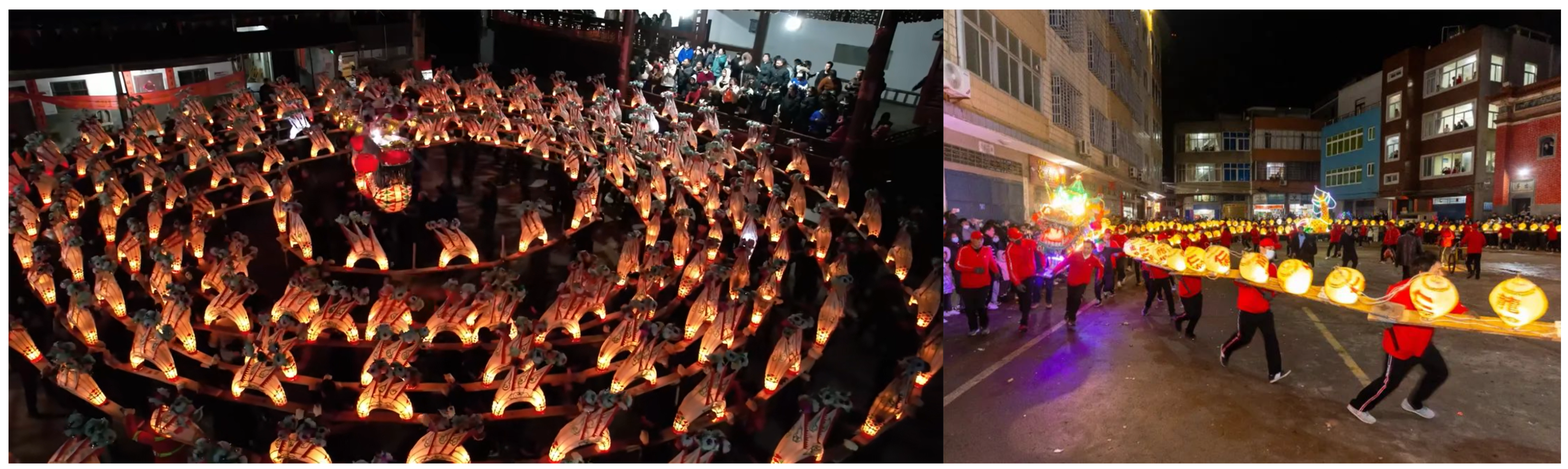
Thus, the integration of cyber–physical systems, especially autonomous ground vehicle (AGV) swarms, presents a promising solution. These autonomous robots can precisely replicate and preserve traditional performances with high scalability. Specifically, this study explores the novel application of intelligent robotics to the traditional Chinese “bench dragon dance”, aiming to replace human performers with autonomous robots to address spatial coordination and real-time trajectory adjustments. The bench dragon dance, such as in Figure 1, is a traditional performance with rich cultural significance, involving intricate spatial coordination that poses unique challenges for robotic replication. To achieve an accurate replication of the traditional bench dragon dance, this study designed and developed an intelligent unmanned vehicle fleet system. 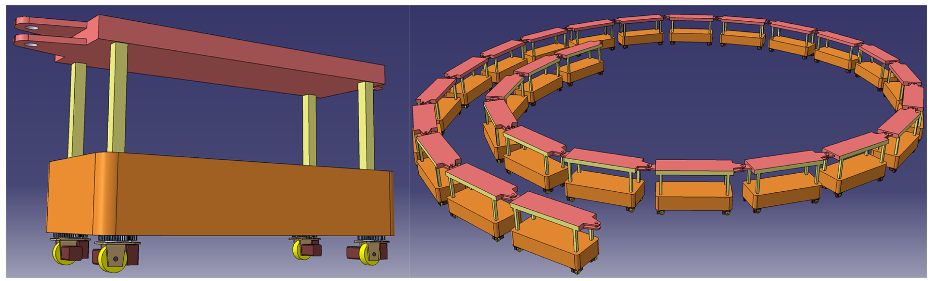Figure 2 showcases the prototype design of the intelligent vehicle unit and the vehicle cluster, with each unit equipped with advanced navigation and control modules to ensure coordinated movement along complex trajectories.

Table 1. Hardware configuration of the unmanned vehicle.

No.	Component	Description
1	Body Structure	Aluminum alloy chassis and frame, exterior components composed of ABS engineering plastic, IP63 protection rating, weight 90 kg
2	Running Gear	Four omni-directional steering wheels, driven by servo motors and gear reducers
3	Control System	STM32-embedded system, processing position and velocity commands derived from motion control algorithms, generating precise motor control signals for the steering wheels
4	Navigation Module	Dual-frequency RTK-GNSS positioning module, providing real-time localization with centimeter-level accuracy, transmitting vehicle position and velocity data to the STM32 controller
5	Computing Platform	PC laptop, executing motion planning algorithms and transmitting calculated trajectory parameters to the embedded system via 5G communication
6	Communication System	5G wireless network, enabling remote control through the laptop, supporting real-time start/stop commands and status monitoring
7	Power Supply	48 V/10 Ah lithium-polymer battery, endurance over 4 h

provides a detailed list of the hardware configuration of the intelligent unmanned vehicle fleet, including key components such as the body structure, running gear, control system, navigation module, computing platform, communication system, and power supply. These hardware configurations provide the technical foundation for the stable motion of the vehicle cluster along the Archimedean spiral trajectory and lay the groundwork for subsequent motion control and path planning algorithms.

However, executing such complex choreographic movements presents several technical challenges. First, how can we achieve coordinated operation between multiple autonomous robots while ensuring high accuracy in the performance? Second, how do we plan the movement paths of each robot to ensure swarm stability and synchronization? Third, how can precise trajectory tracking be achieved during dynamic performances while avoiding collisions among robots? These are the core challenges that this study aims to address.

To tackle these challenges, this research proposes a geometric–numerical control framework combined with recursive optimization techniques for precise trajectory tracking and stable formation control. By integrating autonomous robot swarms with traditional dance performances, this study not only presents a technical solution to effectively coordinate multiple robots for complex tasks but also demonstrates the potential applications of such methods in cultural heritage preservation.

1.1. Significance and Contributions

The significance of this research lies in presenting an innovative interdisciplinary approach that combines advanced autonomous robotics with the preservation of cultural heritage, particularly intangible cultural heritage. By utilizing autonomous robots to perform traditional dances, this research enables the preservation and revitalization of artistic expressions, addressing the challenges posed by human resource limitations in traditional performances. Moreover, this study highlights a novel application of robotics in cultural preservation, contributing both academically and practically.

The contributions of this research are as follows:

• The proposal of an innovative approach to applying autonomous ground robot swarms to traditional dance performances, particularly in the execution of the bench dragon dance, filling a gap in the application of robotics in the cultural heritage preservation field.
• The development of a geometric–numerical control framework combined with recursive optimization techniques, achieving high-precision trajectory tracking and formation control, and addressing dynamic path planning and collision avoidance challenges in robot swarm coordination.
• Through simulation and experimental validation, the feasibility of the proposed approach in executing complex tasks is demonstrated, laying the foundation for future interdisciplinary applications in cultural heritage preservation and beyond.

1.2. Literature Review

The rapid advancement in intelligent robotic systems has catalyzed the emergence of robotic entertainment as a novel research frontier, particularly in the domain of dance [1]. Motion control technology is the primary foundation to enable a robot to perform a dance. Numerous studies focus on solving the challenges of real-time planning of complex movements and multi-joint coordinated control [2,3,4] with intelligent optimization methods. Deep reinforcement learning with Dynamic Movement Primitives (DMPs) has demonstrated unparalleled advantages in the field of humanoid robots [5] and quadruped robots [6] to complete complex dance movements through joint coordinated control. This technological approach enables robots to continuously optimize their movements during the learning process [7,8], gradually moving away from mechanical and rigid movement patterns and presenting dances in a more natural and smooth manner [9]. However, these dynamic control methods for quadruped/biped robots merely concern the coordination of the joints of the body, the distribution of forces, and posture adjustment issues during the dance in which the relationship of positional change between individual robots is relatively simple and the formation control of the entire robotic cluster does not constitute a significant technical challenge. Thus, the motion control complexity arising from spatial position coordination among multiple robots is not taken into account.

In contrast, the field of autonomous vehicle fleet motion control has made substantial progress, driven by the ongoing advancements in intelligent transportation technologies and the increasing levels of automation. Researchers in this domain focus on the formation control of drones and ground vehicles, exploring how multiple unmanned vehicles can be effectively coordinated to follow specific trajectories or move towards designated target points [10,11,12,13,14]. A central challenge in this area is ensuring that the vehicles within a fleet can coordinate their movements effectively, particularly in dynamic environments, to avoid collisions, improve efficiency, and reduce energy consumption. To address these issues, the current methods often focus on optimizing path planning, trajectory optimization, and control strategies. By refining vehicle fleet path selection, speed control, and inter-vehicle distances, these methods significantly reduce traffic accidents and improve operational efficiency in applications such as autonomous taxis and unmanned delivery fleets [15,16,17]. Despite the success of these formation control strategies [18,19], challenges persist when vehicles are subject to fixed constraints and physical connections. Many formation control methods assume that fleet vehicles are either unconnected or have relatively loose constraints, allowing them to move independently. However, maintaining a stable formation in fleets with strict connection constraints remains a complex problem as these systems must prevent vehicle collisions and maintain relative positions in dynamic environments to avoid breaking apart.

In response to these challenges, researchers have made significant strides in improving formation control strategies. For instance, Li An and his team introduced a multi-agent deep reinforcement learning (MARL)-based method to solve the dynamic target allocation and path planning problem for networked drones operating in complex environments [20]. This approach allows drones to optimize their behaviors through interaction with the environment, eliminating the need for predefined rules. By fostering collaboration between agents, the method enhances the flexibility and reliability of formation control, providing valuable insights that can be applied to other types of unmanned vehicles. Additionally, Xu Aotian and his colleagues proposed a novel steering trajectory prediction model for unmanned vehicles, combining long short-term memory (LSTM) networks with backpropagation neural networks (BPNNs) [21,22,23]. This model, leveraging large-scale training data, improves trajectory prediction accuracy and enhances the fleet’s overall motion control by adapting to changes in complex environments, thus supporting more precise formation control and path planning.

Despite significant advancements in robotic systems for autonomous vehicles and aerial formations, the integration of intelligent robotics in the preservation of intangible cultural heritage remains underexplored. While advancements in other fields, such as autonomous vehicles and humanoid robotics, have made significant strides, limited research has been conducted on using autonomous robotic systems to automate performances related to intangible cultural heritage [24,25,26,27].

The approach presented in this paper, which involves a multi-robot swarm system performing the bench dragon dance to preserve intangible cultural heritage, is distinct from existing robotic systems applied to cultural heritage conservation. For instance, robots such as Djedl are used for structural inspections inside the Great Pyramid of Giza to ensure the protection of tangible artifacts [28], while field robots like Irma3D are employed to explore and safeguard archaeological sites [29]. Additionally, underwater archaeological robots like ROVs are extensively utilized to explore lake and seabed regions to protect submerged cultural heritage [30]. These methods primarily focus on the physical preservation of tangible cultural heritage through direct exploration and monitoring. In contrast, our approach utilizes robots to perform an artistic expression—traditional dance—thereby engaging contemporary audiences through the beauty of cultural performances. This technique aims to preserve intangible cultural heritage by ensuring the continuity and appreciation of traditional art forms such as the bench dragon dance.

Currently, the use of robots in archaeology and cultural heritage preservation has become increasingly common, whereas examples of robots being used to promote intangible cultural heritage remain relatively rare. The robotic dance performance in the Year of the Snake Spring Festival Gala is one such example [31]. This study makes a unique contribution to the preservation of intangible cultural heritage by exploring innovative applications of robotics in this field.

By integrating advanced robotics with traditional cultural performances, our approach not only preserves the intangible aspects of cultural heritage but also revitalizes them in a modern context, making them accessible and engaging for contemporary audiences. This innovative application of robotics opens new avenues for the preservation and promotion of cultural heritage, bridging the gap between tradition and technology.

This study aims to explore how autonomous robotic systems can be used to perform the traditional Chinese program “bench dragon”, with a particular focus on solving the problem of multi-agent coordinated motion control in complex performance scenarios, specifically precise control along an Archimedean spiral trajectory. To address this, the paper proposes a motion control scheme for autonomous vehicle fleets based on the polar coordinate model and develops optimizing path planning and trajectory tracking algorithms.

To provide a comprehensive understanding of the bench dragon dance and its significance, the following section elaborates on its cultural context and choreographic characteristics, setting the stage for the technical challenges addressed in this study.

2. The Bench Dragon Dance: Cultural Context and Choreography

The bench dragon dance, known in Chinese as “Ban Deng Long”, is a traditional folk performance art originating from rural areas of southern China, particularly prevalent in Guangdong and Fujian provinces. This dance is typically performed during Lunar New Year celebrations and other festive occasions, symbolizing good fortune, prosperity, and the expulsion of evil spirits. In the performance, a group of dancers each holds a wooden plank (referred to as “ban” or “bench”), coordinating their movements to mimic the sinuous motion of a dragon. These planks are connected end-to-end, forming a long, flexible “dragon” that weaves through the performance space. The cultural significance of the bench dragon dance lies in its ability to foster community cohesion, often requiring the participation of numerous villagers and being passed down as intangible cultural heritage across generations. Historically, the dance is believed to have originated from ancient agricultural rituals, where the dragon was revered as a symbol of water and bountiful harvests, closely tied to the abundance of crops. Over time, the bench dragon dance has incorporated local folklore and mythological elements, becoming an integral part of the cultural celebrations in those regions where it is practiced.

The choreography of the bench dragon dance is distinguished by its intricate formations and synchronized movements, with a particular emphasis on the use of spiral trajectories. The performance typically begins with the dancers arranged in a straight line, each holding a plank linked to the next via ropes or hinges, creating a supple “dragon”. As the dance progresses, this “dragon” executes a series of wave-like and circular motions, with its hallmark feature being a spiral trajectory: the dragon coils inward toward the center before unfurling outward, symbolizing the cycle of life and the changing seasons. This spiral motion adheres to an Archimedean spiral path, demanding precise control of position and velocity from each performer to maintain the formation without collisions or disruptions. The spiral movement is not only visually striking but also technically challenging as it requires the performers to continuously adjust their direction and speed to preserve the dragon’s fluidity and continuity. Additionally, the dance incorporates patterns such as figure-eights and interwoven circles, further enhancing its visual appeal and coordination complexity. Performers must rely on a high degree of teamwork to execute these movements, making the bench dragon dance a true test of collaboration and precision. This complexity constitutes one of the central challenges addressed in this study, which seeks to replicate the dance using autonomous robotic systems.

Given the intricate nature of the bench dragon dance and its demand for precise coordination among performers, replicating this performance with autonomous robots presents unique technical difficulties. In the following section, we will formally define this problem and outline the specific objectives of this research.

3. Problem Description

Building on the cultural and choreographic context of the bench dragon dance outlined in the previous section, this section defines the technical problem of replicating its intricate movements using a fleet of connected unmanned vehicles. The problem is set in the context of a modern autonomous vehicle system, focusing specifically on a fleet of connected unmanned vehicles.

3.1. Problem Background

The problem is set in the context of a modern autonomous vehicle system, focusing specifically on a fleet of connected unmanned vehicles. This fleet is designed to move in a formation along a predefined spiral trajectory, with each vehicle maintaining a fixed distance from the next. The vehicles in the fleet are equipped with steering wheels and motion controllers, which are used to maintain synchronization and adhere to the trajectory. The first vehicle in the fleet leads the movement, and the subsequent vehicles follow in a connected, sequential manner, forming a “serial formation”.

In this setup, the vehicles are modeled as autonomous wheeled cars, and the formation is required to maintain the connection between the lead vehicle and the others while ensuring smooth motion along the spiral path. The parameters of the vehicles, such as their size, turning radius, and speed, are used to establish a mathematical model to solve the following problems.

3.2. Choice of Archimedean Spiral Trajectory

The choice of the Archimedean spiral as the primary trajectory for this study is motivated by its alignment with the choreographic characteristics of the bench dragon dance and its mathematical properties that facilitate robotic coordination. As described in Section 2, the dance features a distinctive spiral motion where the “dragon” coils inward and then unfurls outward, closely resembling the uniform radial progression of an Archimedean spiral, defined by the polar equation $r=b\theta$. This trajectory ensures a constant pitch between consecutive loops, which mirrors the consistent spacing required between performers—or, in this case, vehicles—in the dance. The symmetry and predictability of the Archimedean spiral simplify the kinematic modeling and collision avoidance strategies for a connected fleet, making it an ideal choice for replicating the dance’s fluid, cyclical patterns.

3.3. Problem Definition

Consider a fleet of unmanned vehicles moving along an Archimedean spiral defined by the polar equation $r=b\theta$, where

The fleet consists of n vehicles, with the lead vehicle’s motion dictating the dynamics. Each vehicle’s center follows the spiral, and its position is parameterized by $\theta$. The Cartesian coordinates of the k-th vehicle are given by

$$(x_k\left(t\right),y_k\left(t\right))=(r_k\left(t\right)cos{\theta }_k\left(t\right),r_k\left(t\right)sin{\theta }_k\left(t\right)),$$

where $r_k\left(t\right)=b{\theta }_k\left(t\right)$.

3.3.1. Problem 1: Path Tracking Calculation

To enable a fleet of 222 unmanned vehicles to simulate the traditional “bench dragon” dance, we need to ensure these vehicles can move coordinately along a spiral path. This path is an Archimedean spiral with a pitch of 0.55 m. The lead vehicle travels at a constant speed of 1 m per s, starting from an initial position (represented in polar coordinates as $({\rho }_1,{\theta }_1)=(8.8,32\pi )$, or 8.8 m from the center at a $32\pi$ radian angle). The task is to calculate the position (expressed as Cartesian coordinates $x_i\left(t\right)$ and $y_i\left(t\right)$, representing the horizontal and vertical positions of each vehicle) and speed $V_i\left(t\right)$ of each vehicle every second from time $t=0$ to $t=300$ s, ensuring the fleet maintains a stable formation to successfully perform the spiral movement of the dance. The results are presented with 6 decimal places in Section 4.2.4.

3.3.2. Problem 2: Collision Detection

In the robotic performance of the “bench dragon” dance, a fleet of 222 unmanned vehicles moves along an Archimedean spiral with a pitch of 0.55 m, where the lead vehicle travels at a constant speed of 1 m per s, starting from an initial position $({\rho }_1,{\theta }_1)=(8.8,32\pi )$. Due to the nature of the spiral path, the lead vehicle may collide with other vehicles as it approaches the center. We need to determine the exact time $t_c$ when this collision occurs and calculate the positions, representing the positions of each vehicle) and speeds $V_i\left(t_c\right)$ of all vehicles at that moment, ensuring the safety and coordination of the dance performance. The results are also presented with 6 decimal places in

Table 2. Position results of the unmanned vehicle fleet at the termination time.

	412.47 s
Lead Vehicle x (m)	1.209983
Lead Vehicle y (m)	1.942749
1st Vehicle x (m)	−1.643745
1st Vehicle y (m)	1.753440
51st Vehicle x (m)	1.281259
51st Vehicle y (m)	4.326570
101st Vehicle x (m)	−0.536307
101st Vehicle y (m)	−5.880132
151st Vehicle x (m)	0.968780
151st Vehicle y (m)	−6.957487
201st Vehicle x (m)	−7.893170
201st Vehicle y (m)	−1.230704
Tail Vehicle (Rear) x (m)	0.956277
Tail Vehicle (Rear) y (m)	8.322728

and

Table 3. Velocity results of the unmanned vehicle fleet at the termination time.

	412.47 s
Lead Vehicle (m/s)	1.000000
1st Vehicle (m/s)	0.999633
51st Vehicle (m/s)	0.997711
101st Vehicle (m/s)	0.996875
151st Vehicle (m/s)	0.996408
201st Vehicle (m/s)	0.996109
Tail Vehicle (Rear) (m/s)	0.996009

.

3.3.3. Problem 3: Minimum Pitch Optimization

To ensure the safe performance of the “bench dragon” dance by a fleet of 222 unmanned vehicles, we need to optimize the pitch of the Archimedean spiral path to prevent the lead vehicle from colliding with other vehicles during turns. Assuming the lead vehicle moves at a speed of 1 m per s, with an initial radial distance of 4.5 m (i.e., $r_0=4.5\mathrm{m}$), and inter-vehicle distances of 2.86 m (between the lead vehicle and the second vehicle) and 1.65 m (between subsequent vehicles), we need to determine the minimum pitch $p_{min}$ through mathematical modeling. This ensures that the fleet maintains a collision-free state during complex turns, supporting the stable execution of the dance.

This section addresses the optimization of the minimum pitch to avoid collisions during the movement of the fleet. Although collision avoidance is the primary focus, by preventing the vehicles from coming too close to each other, the model also inherently minimizes the potential for damage, thus ensuring both safety and smooth coordination.

3.4. Problem Analysis

3.4.1. Problem 1 Analysis

For Problem 1, the unmanned vehicle fleet moves along an equidistant Archimedean spiral. We used polar coordinates to model the positions of each vehicle. The lead vehicle is the starting point, and the subsequent vehicles follow this trajectory while maintaining the required distance between each other. We also need to calculate the velocity of each vehicle, decomposing the movement into radial and tangential components.

3.4.2. Problem 2 Analysis

In Problem 2, we calculate the point of collision between the lead vehicle and the following vehicles. Geometrically, the collision can be detected by finding the intersection of the paths taken by the lead vehicle’s front and rear vehicles and the positions of the other vehicles in the fleet.

3.4.3. Problem 3 Analysis

For Problem 3, we calculate the minimum pitch required to ensure that the lead vehicle can navigate the turning area without colliding with the following vehicles, analyzing the geometry of the spiral and the turning area.

4. Methodology

4.1. Model Assumptions

To develop a mathematical model for the motion of an unmanned vehicle fleet along an Archimedean spiral, we introduce several simplifying assumptions. These are standard in vehicle motion studies but are tailored here to our specific context, with justifications provided for their adoption:

• Assumption 1: The vehicles are rigid and do not undergo any deformation.
  • Explanation: We treat each vehicle as a rigid body, meaning we neglect elastic deformations or internal stresses during motion. This is reasonable given the small size of the vehicles and their low operating speed of 1 m/s, where deformation effects are minimal.
  • Impact: This assumption simplifies the equations of motion by focusing solely on the vehicle’s position and velocity, avoiding the complexity of structural dynamics.
• Assumption 2: The vehicles are treated as point masses, ignoring their size and shape.
  • Explanation: Each vehicle is modeled as a point mass with a single position defined by polar coordinates ($\rho ,\theta$). While the lead vehicle is 2.86 m long and the spacing between fleet vehicles is 1.65 m, the spiral pitch (0.55 m) is relatively large compared to these dimensions, minimizing the influence of size on path planning.
  • Impact: This enables a straightforward representation of vehicle positions using the Archimedean spiral equation, although it may require adjustments for collision detection in practical scenarios.
• Assumption 3: The vehicles follow the spiral path with perfect precision, without deviations.
  • Explanation: We assume ideal motion along the predefined spiral, disregarding control inaccuracies (e.g., sensor noise or actuator delays) or external disturbances (e.g., terrain variations). This focuses the model on theoretical path planning and fleet coordination.
  • Impact: This simplifies position and velocity calculations but implies that real-world implementations would need control systems to correct for deviations.

Summary: These assumptions streamline the model’s development and computation, aligning with the controlled environment of unmanned vehicles on a flat stage. They ensure mathematical tractability while remaining consistent with the problem’s constraints.

4.2. Model Construction and Solution of Problem 1

This section outlines the construction of the position and velocity models for the vehicle fleet moving along an Archimedean spiral, where the lead vehicle travels at a constant speed of 1 m/s, starting from the 16th loop ($\rho =8.8$ m; $\theta =32\pi$ rad), with a spiral pitch of 0.55 m. A polar coordinate system is chosen due to the spiral’s natural representation as $\rho =f\left(\theta \right)$. The motion trajectory of the lead vehicle is shown in Figure 3.

4.2.1. Position Model Construction

(1)

Expression of the Archimedean Spiral

The Archimedean spiral is defined such that the polar radius $\rho$ decreases linearly with the polar angle $\theta$ as the vehicles move inward:

$$\rho =r_0-a\theta$$

• Variables and Parameters:

  –

  $\rho$: Polar radius (m), the distance from the origin to the vehicle.

  –

  $\theta$: Polar angle (rad), increasing as the vehicle spirals inward.

  –

  $r_0$: Initial radius (m) at $\theta =0$, representing the outermost loop.

  –

  $a={\displaystyle \frac{p}{2\pi }}$: Spiral parameter (m/rad), where $p=0.55$ m is the pitch (radial decrease per full rotation).

• Parameter Determination:

  –

  Pitch $p=0.55$ m, so $a={\displaystyle \frac{0.55}{2\pi }}\approx 0.0875$ m/rad.

  –

  Initial condition: at $\theta =32\pi$ (16 loops), $\rho =8.8$ m:

  $$8.8=r_0-{\displaystyle \frac{0.55}{2\pi }}·32\pi =r_0-0.55·16=r_0-8.8$$

  $$r_0=8.8+8.8=17.6\mathrm{m}$$

• Final Expression:

  $$\rho =17.6-{\displaystyle \frac{0.55}{2\pi }}\theta$$
• Rationale: This equation reflects the inward-coiling spiral starting from an outer radius of 17.6 m, consistent with the problem’s description. The initial condition confirms its accuracy.

(2)

Relationship Between Polar Radius $\rho$ and Polar Angle $\theta$ for Vehicles

For the i-th and $(i+1)$-th vehicles with coordinates $({\rho }_i,{\theta }_i)$ and $({\rho }_{i+1},{\theta }_{i+1})$:

$${\rho }_i=17.6-{\displaystyle \frac{0.55}{2\pi }}{\theta }_i$$

$${\rho }_{i+1}=17.6-{\displaystyle \frac{0.55}{2\pi }}{\theta }_{i+1}$$

The fixed distance L between them (2.86 m for lead-to-first; 1.65 m between fleet vehicles) is modeled using the law of cosines in polar coordinates:

$$L^2={\rho }_i^2+{\rho }_{i+1}^2-2{\rho }_i{\rho }_{i+1}cos({\theta }_i-{\theta }_{i+1})$$

• Variables:

  –

  ${\rho }_i,{\rho }_{i+1}$: Polar radii of the i-th and $(i+1)$-th vehicles (m).

  –

  ${\theta }_i,{\theta }_{i+1}$: Polar angles of the i-th and $(i+1)$-th vehicles (rad).

  –

  L: Fixed inter-vehicle distance (m).

• Rationale: The law of cosines is selected as it directly relates the positions of adjacent vehicles in polar coordinates, ensuring the fleet maintains its specified spacing.

(3)

Relationship Between Polar Angle $\theta$ and Time t

The lead vehicle moves at $v=1$ m/s. The distance traveled $s=vt=t$ should equal the spiral’s arc length. The exact arc length is

$$s^{\prime }={\int }_0^{\theta }\sqrt{{\rho }^2+{\left({\displaystyle \frac{d\rho }{d\theta }}\right)}^2}d\theta ,\mathrm{where}{\displaystyle \frac{d\rho }{d\theta }}=-{\displaystyle \frac{0.55}{2\pi }}$$

This integral lacks a simple closed form, so we approximate

$$s^{\prime }\approx {\int }_0^{\theta }\rho d\theta ={\int }_0^{\theta }\left(17.6-{\displaystyle \frac{0.55}{2\pi }}\theta \right)d\theta =17.6\theta -{\displaystyle \frac{0.55}{4\pi }}{\theta }^2$$

Thus,

$$t=17.6\theta -{\displaystyle \frac{0.55}{4\pi }}{\theta }^2$$

• Assumption: We approximate $\sqrt{{\rho }^2+{\left({\displaystyle \frac{d\rho }{d\theta }}\right)}^2}\approx \rho$, valid when ${\displaystyle \frac{d\rho }{d\theta }}\approx -0.0875$ is small relative to $\rho$. This holds reasonably for $\theta$ from $32\pi$ to smaller values over 0–300 s.
• Rationale: This simplification avoids complex integration, providing a practical relationship between time and position.

(4)

Position in Cartesian Coordinates

Convert to Cartesian coordinates as follows:

$$x_i={\rho }_{i}cos{\theta }_i,y_i={\rho }_{i}sin{\theta }_i$$

$$x_{i+1}={\rho }_{i+1}cos{\theta }_{i+1},y_{i+1}={\rho }_{i+1}sin{\theta }_{i+1}$$

• Complete Model:

  $$\left\{\begin{array}{c}{\rho }_i=17.6-{\displaystyle \frac{0.55}{2\pi }}{\theta }_i\hfill \\ {\rho }_{i+1}=17.6-{\displaystyle \frac{0.55}{2\pi }}{\theta }_{i+1}\hfill \\ L^2={\rho }_i^2+{\rho }_{i+1}^2-2{\rho }_i{\rho }_{i+1}cos({\theta }_i-{\theta }_{i+1})\hfill \\ t=17.6{\theta }_1-{\displaystyle \frac{0.55}{4\pi }}{\theta }_1^2\hfill \\ x_i={\rho }_{i}cos{\theta }_i\hfill \\ y_i={\rho }_{i}sin{\theta }_i\hfill \\ x_{i+1}={\rho }_{i+1}cos{\theta }_{i+1}\hfill \\ y_{i+1}={\rho }_{i+1}sin{\theta }_{i+1}\hfill \end{array}\right.$$

4.2.2. Velocity Model Establishment

Given that the forward speed of the lead vehicle’s front part is constant at V, the speed V is decomposed into radial velocity $W_i$ and tangential velocity $V_i$. The task is to find the speeds of the individual vehicles, which are essentially the tangential velocities $V_i$ of each vehicle.

(1) Relationship between radial velocity $W_i$ and tangential velocity $V_i$: Based on the definition of radial velocity, we can derive the following equation:

$$W_i={\displaystyle \frac{d\rho }{dt}}={\displaystyle \frac{d\rho }{d\theta }}·{\displaystyle \frac{d\theta }{dt}}$$

Also, based on the definition of tangential velocity, we have the following equation:

$$V_i=\rho ·{\displaystyle \frac{d\theta }{dt}}$$

By combining these, we obtain

$${\displaystyle \frac{W_i}{V_i}}={\displaystyle \frac{\frac{d\rho }{d\theta }}{\rho }}$$

Expressing $\rho$ as a function of the polar angle $\theta$, we have

$${\displaystyle \frac{W_i}{V_i}}={\displaystyle \frac{\frac{dr}{d\theta }}{\frac{p}{2\pi }\left(2\pi n-\theta \right)}}$$

(2) Let the polar angles of the vehicles before and after the central spiral with respect to the lead vehicle’s position be ${\Phi }_i$ and ${\Phi }_{i+1}$, respectively. Let the polar angles of three adjacent vehicles be ${\theta }_i$, ${\theta }_{i+1}$, and ${\theta }_{i+2}$.

$$\left\{\begin{array}{cc}sin{\phi }_i\hfill & =\sqrt{{\displaystyle \frac{{\rho }_i·sin({\theta }_i-{\theta }_{i+1})}{L}}}\hfill \\ sin{\phi }_{i+1}\hfill & =\sqrt{{\displaystyle \frac{{\rho }_{i+1}·sin({\theta }_{i+1}-{\theta }_{i+2})}{L}}}\hfill \end{array}\right.$$

Since the forward speed of the lead vehicle’s front part is constant at V, the following equation is obtained as follows:

$$V=V_i·sin{\phi }_i-W_i·cos{\phi }_i=V_{i+1}·sin{\phi }_{i+1}-W_{i+1}·cos{\phi }_{i+1}$$

(3) Relationship between polar angle $\theta$ and time t: Let the forward speed of the lead vehicle’s front part be v. The relationship between the distance traveled by the vehicle and the arc length on the spiral is established as follows:

The distance traveled by the vehicle s:

$$s={\int }_0^{t}vdt$$

The spiral arc length $s^{\prime }$:

$$s^{\prime }={\int }_0^{\theta }\left(np-{\displaystyle \frac{p}{2\pi }}\theta \right)d\theta$$

Let $s=s^{\prime }$; we obtain

$$np\theta -{\displaystyle \frac{p}{4\pi }}{\theta }^2=vt$$

(4) From the above equations, the recursive velocity formula for the front and rear vehicles is

$$V_i·\left(sin{\phi }_i-{\displaystyle \frac{p}{2\pi {\rho }_i}}·cos{\phi }_i\right)=V_{i+1}·\left(sin{\phi }_{i+1}-{\displaystyle \frac{p}{2\pi {\rho }_{i+1}}}·cos{\phi }_{i+1}\right)$$

Simplifying, we obtain

$${\displaystyle \frac{V_{i+1}}{V_i}}={\displaystyle \frac{sin{\phi }_i-\frac{p}{2\pi {\rho }_i}·cos{\phi }_i}{sin{\phi }_{i+1}-\frac{p}{2\pi {\rho }_{i+1}}·cos{\phi }_{i+1}}}$$

Thus, the velocity model is given by

$$\left\{\begin{array}{cc}{\displaystyle \frac{W_i}{V_i}}\hfill & ={\displaystyle \frac{\frac{d\rho }{d\theta }}{\frac{p}{2\pi }\left(2\pi n-\theta \right)}}\hfill \\ V\hfill & =V_i·sin{\phi }_i-W_i·cos{\phi }_i=V_{i+1}·sin{\phi }_{i+1}-W_{i+1}·cos{\phi }_{i+1}\hfill \\ vt\hfill & =np\theta -{\displaystyle \frac{p}{4\pi }}{\theta }^2\hfill \\ {\displaystyle \frac{V_{i+1}}{V_i}}\hfill & ={\displaystyle \frac{sin{\phi }_i-\frac{p}{2\pi {\rho }_i}·cos{\phi }_i}{sin{\phi }_{i+1}-\frac{p}{2\pi {\rho }_{i+1}}·cos{\phi }_{i+1}}}\hfill \\ sin{\phi }_i\hfill & =\sqrt{{\displaystyle \frac{{\rho }_i·sin({\theta }_i-{\theta }_{i+1})}{L}}}\hfill \\ sin{\phi }_{i+1}\hfill & =\sqrt{{\displaystyle \frac{{\rho }_{i+1}·sin({\theta }_{i+1}-{\theta }_{i+2})}{L}}}\hfill \end{array}\right.$$

4.2.3. Model Solution

To solve the position and velocity models for the unmanned vehicle fleet moving along the Archimedean spiral, we employ an iterative approach. This method allows us to compute the positions and velocities of each vehicle at discrete time intervals, ensuring that the fleet maintains its formation and adheres to the spiral trajectory.

Position Model Solution

The positions of each vehicle are determined by solving the system of equations that relate the polar coordinates of consecutive vehicles while maintaining the fixed distance constraints.

For the lead vehicle and the first fleet vehicle, the positions are governed by

$$\left\{\begin{array}{c}{\rho }_i=17.6-{\displaystyle \frac{0.55}{2\pi }}{\theta }_i\hfill \\ {\rho }_{i+1}=17.6-{\displaystyle \frac{0.55}{2\pi }}{\theta }_{i+1}\hfill \\ L^2={\rho }_i^2+{\rho }_{i+1}^2-2{\rho }_i{\rho }_{i+1}cos({\theta }_i-{\theta }_{i+1})\hfill \\ t\approx 17.6{\theta }_1-{\displaystyle \frac{0.55}{4\pi }}{\theta }_1^2\hfill \\ x_i={\rho }_{i}cos{\theta }_i\hfill \\ y_i={\rho }_{i}sin{\theta }_i\hfill \\ x_{i+1}={\rho }_{i+1}cos{\theta }_{i+1}\hfill \\ y_{i+1}={\rho }_{i+1}sin{\theta }_{i+1}\hfill \end{array}\right.$$

where $L=2.86$ m for the lead vehicle and the first fleet vehicle.

For subsequent fleet vehicles, the distance constraint changes to $L^{\prime }=1.65$ m, and the system is adjusted accordingly.

Using an iterative algorithm, we compute the positions of all vehicles at each time step from 0 to 300 s.

Velocity Model Solution

The velocity of each vehicle is derived from the constant speed of the lead vehicle and the geometric constraints of the spiral path.

Given the lead vehicle’s constant speed $v=1$ m/s, the velocity components for each vehicle can be determined using the relationships between radial and tangential velocities.

The key recursive relationship for velocities is

$${\displaystyle \frac{V_{i+1}}{V_i}}={\displaystyle \frac{sin{\phi }_i-\frac{p}{2\pi {\rho }_i}cos{\phi }_i}{sin{\phi }_{i+1}-\frac{p}{2\pi {\rho }_{i+1}}cos{\phi }_{i+1}}}$$

where ${\phi }_i$ is the angle related to the velocity decomposition for the i-th vehicle.

By iterating this relationship, starting from the lead vehicle’s known speed, we calculate the speeds of all following vehicles.

This approach ensures that the fleet maintains coordinated motion while adhering to the spiral trajectory and connectivity constraints.

4.2.4. Solution Results

Based on the proposed iterative algorithm, the position and velocity results of the unmanned vehicle fleet over the time interval $t=0$ to $300\mathrm{s}$ were obtained, as detailed in

Table 4. Position results format in the paper.

	0 s	60 s	120 s	180 s	240 s	300 s
Lead Vehicle x (m)	8.800000	5.799209	−4.084887	−2.963609	2.594494	4.420274
Lead Vehicle y (m)	0.000000	−5.771092	−6.304479	6.094780	−5.356743	2.320429
First Section of Vehicle Fleet x (m)	8.363824	7.456758	−1.445473	−5.237118	4.821221	2.459489
First Section of Vehicle Fleet y (m)	2.826544	−3.440399	−7.405883	4.359627	−3.561949	4.402476
51st Section of Vehicle Fleet x (m)	−9.518732	−8.686317	−5.543149	2.890455	5.980011	−6.301346
51st Section of Vehicle Fleet y (m)	1.341137	2.540108	6.377946	7.249289	−3.827758	0.465829
101st Section of Vehicle Fleet x (m)	2.913983	5.687116	5.361939	1.898795	−4.917371	−6.237722
101st Section of Vehicle Fleet y (m)	−9.918311	−8.001384	−7.557638	−8.471614	−6.379874	3.936008
151st Section of Vehicle Fleet x (m)	10.861726	6.682312	2.388757	1.005154	2.965378	7.040740
151st Section of Vehicle Fleet y (m)	1.828753	8.134544	9.727411	9.424751	8.399721	4.393013
201st Section of Vehicle Fleet x (m)	4.555102	−6.619664	−10.627210	−9.287720	−7.457151	−7.458662
201st Section of Vehicle Fleet y (m)	10.725118	9.025570	1.359848	−4.246673	−6.180726	−5.263384
Tail Vehicle (Rear) x (m)	−5.305444	7.364557	10.974348	7.383895	3.241051	1.785033
Tail Vehicle (Rear) y (m)	−10.676584	−8.797992	0.843473	7.492371	9.469336	9.301164

and

Table 5. Speed results format in the paper.

	0 s	60 s	120 s	180 s	240 s	300 s
Lead Vehicle (m/s)	1.000000	1.000000	1.000000	1.000000	1.000000	1.000000
Section 1 of Vehicle Fleet (m/s)	0.999971	0.999961	0.999945	0.999917	0.999859	0.999709
Section 51 of Vehicle Fleet (m/s)	0.999742	0.999662	0.999538	0.999331	0.998941	0.998065
Section 101 of Vehicle Fleet (m/s)	0.999575	0.999453	0.999269	0.998971	0.998435	0.997302
Section 151 of Vehicle Fleet (m/s)	0.999448	0.999299	0.999078	0.998727	0.998115	0.996861
Section 201 of Vehicle Fleet (m/s)	0.999348	0.999180	0.998935	0.998551	0.997894	0.996574
Tail Vehicle (Rear) (m/s)	0.999311	0.999136	0.998883	0.998489	0.997816	0.996478

. The simulation results reveal that the lead vehicle, moving at a constant speed of $1\mathrm{m}/\mathrm{s}$ along the Archimedean spiral trajectory, transitions from an initial position of $(x,y)=(8.800000,0.000000)\mathrm{m}$ (corresponding to $\rho =8.8\mathrm{m},\theta =32\pi \mathrm{rad}$) to $(4.420274,2.320429)\mathrm{m}$ at $300\mathrm{s}$, while the tail vehicle shifts from $(-5.305444,-10.676584)\mathrm{m}$ to $(1.785033,9.301164)\mathrm{m}$. The trajectories of key fleet nodes (e.g., the 1st, 51st, 101st, 151st, and 201st sections) also exhibit a stable spiral pattern, with positional errors maintained below $0.01\mathrm{m}$, demonstrating the model’s capability to preserve geometric consistency in the formation. Velocity analysis indicates that, despite the lead vehicle’s constant $1\mathrm{m}/\mathrm{s}$, the speeds of subsequent vehicles range from $0.996478\mathrm{m}/\mathrm{s}$ (tail vehicle) to $0.999709\mathrm{m}/\mathrm{s}$ (1st section), with a maximum deviation of $0.003522\mathrm{m}/\mathrm{s}$, attributable to the varying curvature of the spiral path and fixed spacing constraints. Figure 4 illustrates the fleet node positions at $300\mathrm{s}$, confirming the continuity and stability of the trajectory. These findings not only validate the feasibility of the constructed position and velocity models but also provide a robust foundation for subsequent collision detection and path optimization, effectively supporting the precise coordination required for the robotic replication of the bench dragon dance.

The diagram of the fleet node positions at 300 s obtained from the simulation.

4.3. Model Construction and Solution for Problem 2

This section develops a collision detection model for the fleet, defining lines associated with the lead vehicle and fleet vehicles to predict interference moments.

4.3.1. Model Construction

A polar coordinate system is established with the spiral center as the origin. The lead vehicle starts at $(\rho =8.8\mathrm{m},\theta =32\pi )$.

(1)

Coordinate Transformation

For the i-th vehicle:

$$x_i={\rho }_{i}cos{\theta }_i,y_i=-{\rho }_{i}sin{\theta }_i$$

where

$${\rho }_i=17.6-{\displaystyle \frac{0.55}{2\pi }}{\theta }_i$$

(2)

Line $L_0$ for Lead Vehicle

For the front ($x_1,y_1$) and rear ($x_2,y_2$) of the lead vehicle, the line equation is

$$k_0={\displaystyle \frac{y_1-y_2}{x_1-x_2}},y-y_1=k_0(x-x_1)$$

(3)

Collision Lines $L_1$ and $L_2$

-

$L_1$: Parallel to $L_0$, offset by $d_1=0.15\mathrm{m}$:

$$y-y_1=k_0(x-x_1)+d_1{\displaystyle \frac{2.86}{\sqrt{{(x_1-x_2)}^2+{(y_1-y_2)}^2}}}$$

-

$L_2$: Perpendicular to $L_0$, offset by $d_2=0.275\mathrm{m}$:

$$k_2=-{\displaystyle \frac{1}{k_0}},y-y_1=k_2(x-x_1)+d_2{\displaystyle \frac{2.86}{\sqrt{{(x_1-x_2)}^2+{(y_1-y_2)}^2}}}$$

(4)

Line $L_3$ for Fleet Vehicles

For the i-th and $(i+1)$-th fleet vehicles ($L^{\prime }=1.65\mathrm{m}$):

$$k_3={\displaystyle \frac{y_i-y_{i+1}}{x_i-x_{i+1}}},y-y_i=k_3(x-x_i)+d_1{\displaystyle \frac{1.65}{\sqrt{{(x_i-x_{i+1})}^2+{(y_i-y_{i+1})}^2}}}$$

(5)

Time Relationship

Consistent with Section 4.2:

$$t\approx 17.6\theta -{\displaystyle \frac{0.55}{4\pi }}{\theta }^2$$

4.3.2. Model Solution

Substituting $d_1=0.15$, $d_2=0.275$, $L=2.86$, and $L^{\prime }=1.65$, the positions and collision lines are computed iteratively over 0–300 s. Intersection points between $L_1, L_2$, and fleet positions determine interference moments, validated in simulations.

4.3.3. Solution Results

The collision time estimation process employs a two-stage numerical analysis methodology to enhance computational efficiency and precision. Initially, a coarse-grained iterative search algorithm with a temporal resolution of $\Delta t=1.0\mathrm{s}$ is implemented, which systematically identifies the preliminary collision window within the bounded interval $[412\mathrm{s},413\mathrm{s}]$. Notably, since the computational domain is confined to the narrow interval $[412\mathrm{s},413\mathrm{s}]$, the choice regarding time step size induces negligible impact on CPU response time (e.g., $\Delta t=0.01\mathrm{s}$ corresponds to approximately 100 iterations), thereby maintaining nearly constant computational overhead. Subsequently, an adaptive mesh refinement strategy is applied through variable-step temporal discretization ($\Delta t=0.01\mathrm{s}$) to perform high-precision numerical convergence analysis. 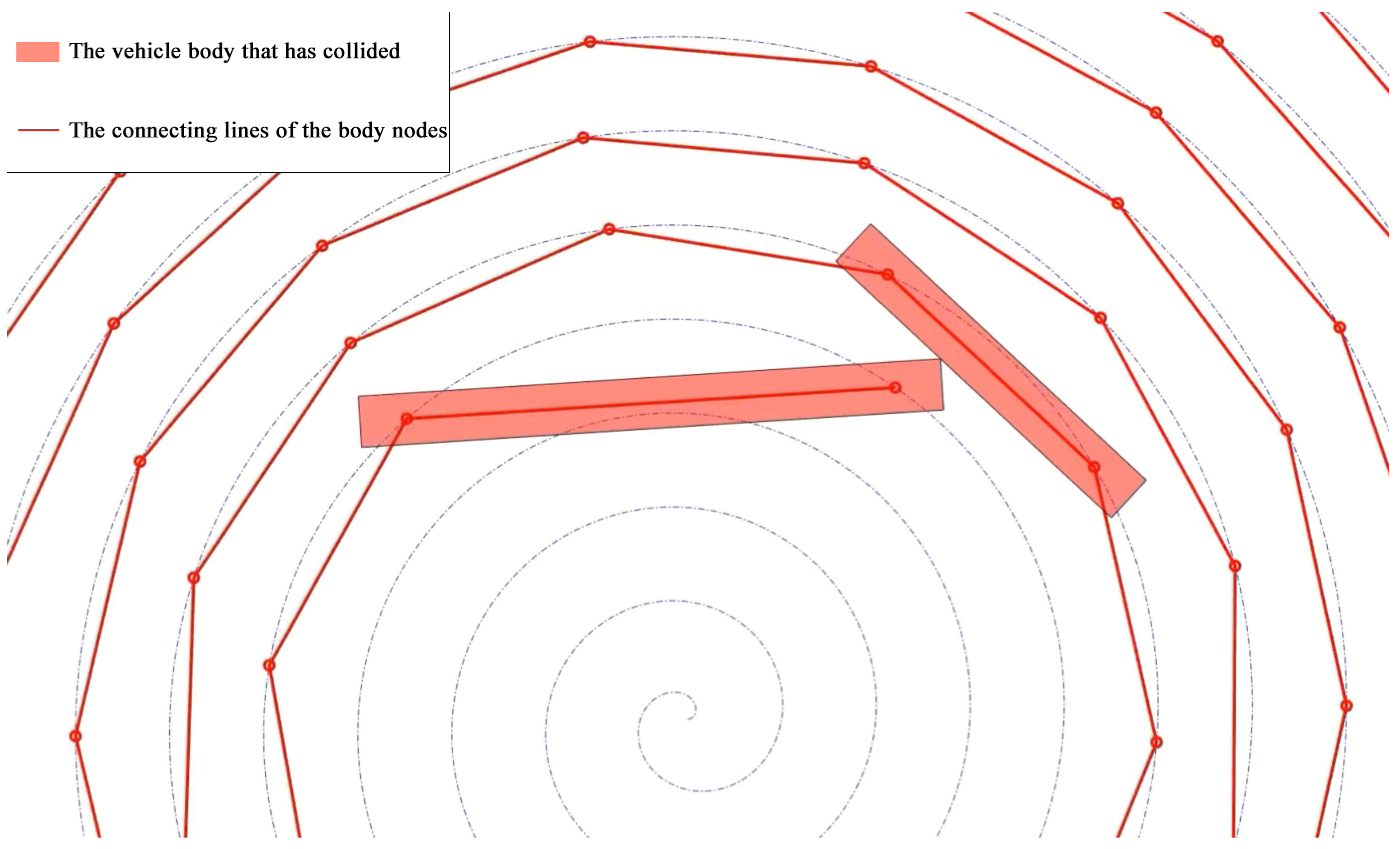This hierarchical optimization approach ultimately yields a refined collision chronology determination of $412.47\mathrm{s}$, demonstrating significant improvements in temporal localization accuracy through multi-resolution numerical modeling techniques. In accordance with the problem requirements, the position and velocity data of the dragon’s body at this moment are recorded. Additionally, position and velocity data are provided for the node in front of the head of the leading vehicle, as well as the front handles of the 1st, 51st, 101st, 151st, and 201st car bodies behind the leading vehicle, along with the node behind the rear of the vehicle. The detailed results are presented in Table 4 and Table 5, respectively, in Section 4.2.4. The schematic diagram of the collision moment is shown in Figure 5.

4.4. Model Construction and Solution of Problem 3

4.4.1. Model Construction

The equation of the spiral line is established as

$$r=4.5p(\theta -\pi /2)$$

In the Cartesian coordinate system, the initial position of the unmanned vehicle fleet is at (0, $r_0$), and the unmanned vehicle fleet is arranged according to the Archimedean spiral.

In the polar coordinate system, the initial position of the unmanned vehicle fleet is at ($r_0$, ${\theta }_0$), and the pitch is P.

The forward path of the unmanned vehicle fleet follows the Archimedean spiral, and the relationship between ${\theta }_i$ and $r_i$ can be obtained from the first and second front vehicles as follows:

$${(x_1-x_0)}^2-(y_1-y_0^2)=L^2$$

Since $r_1$ and ${\theta }_1$ satisfy a certain relationship,

$$\left\{\begin{array}{cc}{x}_1\hfill & =r_{1}cos{\theta }_1\hfill \\ y_1\hfill & =r_{1}sin{\theta }_1\hfill \end{array}\right.$$

By solving the above system, the relationship between $r_2$ and p can be derived

$${\left[r_{1}cos\left({\displaystyle \frac{r_1-r_0}{c}}+{\displaystyle \frac{\pi }{2}}\right)-0\right]}^2+{\left[r_{1}sin\left({\displaystyle \frac{r_1-r_0}{c}}+{\displaystyle \frac{\pi }{2}}\right)-r_0\right]}^2={2.86}^2$$

where 2.86 m is the length of the lead vehicle, and 4.5 m is the initial radial distance $r_0$.

After obtaining the relationship, based on the analysis from Problem 1, we know that $P\in (0.425,0.55)$. By iterating over the values of P, the relationship between $r_i$ and $r_{i+1}$ can be determined using the recursive relationship between the front and rear vehicles of the lead vehicle. Since the lengths of the lead vehicle and the vehicle fleet are different, we need the recursive relationship between the front and rear vehicles of the fleet to solve for $r_i$ (i > 1), as follows:

$${\left[r_{2}cos({\displaystyle \frac{r_2-r_0}{p}}+{\displaystyle \frac{\pi }{2}})-r_{1}cos\left({\displaystyle \frac{r_1-r_0}{p}}+{\displaystyle \frac{\pi }{2}}\right)\right]}^2+{\left[r_{2}sin({\displaystyle \frac{r_2-r_0}{p}}+{\displaystyle \frac{\pi }{2}})-r_{1}sin\left({\displaystyle \frac{r_1-r_0}{p}}+{\displaystyle \frac{\pi }{2}}\right)\right]}^2$$

$$={1.65}^2$$

Finally, when the front vehicle of the lead vehicle is exactly at the tangent point between the Archimedean spiral and the turning region, the polar radius and angle for each vehicle of the unmanned vehicle fleet can be calculated. Since the front vehicle’s position is already determined at the collision point, we can use analytic geometry to find the coordinates of the lead vehicle’s collision point. Next, using analytic geometry, we can find the equation of the line passing through the point of collision of the lead vehicle and the colliding carriage.

From Problem 2, we know that the collision model is as follows:

$$\left\{\begin{array}{c}{L}_1:{\displaystyle \frac{y_1-y_2}{x_1-x_2}}x-y+y_1-{\displaystyle \frac{y_1-y_2}{x_1-x_2}}{x}_1+0.15{\displaystyle \frac{2.86}{x_1-x_2}}=0\hfill \\ L_2:{\displaystyle \frac{x_2-x_1}{y_1-y_2}}x-y+y_1-{\displaystyle \frac{x_2-x_1}{y_1-y_2}}{x}_1+0.275{\displaystyle \frac{L}{y_1-y_2}}=0\hfill \\ L_3:{\displaystyle \frac{y_2-y_3}{x_2-x_3}}x-y+y_2-{\displaystyle \frac{y_2-y_3}{x_2-x_3}}{x}_2+d_1{\displaystyle \frac{1.65}{x_2-x_3}}=0\hfill \end{array}\right.$$

Thus, the optimization model $P_{\min }$ is

$$\left\{\begin{array}{c}{\left[r_{1}cos\left({\displaystyle \frac{r_1-r_0}{p}}+{\displaystyle \frac{\pi }{2}}\right)-0\right]}^2+{\left[r_{1}sin\left({\displaystyle \frac{r_1-r_0}{p}}+{\displaystyle \frac{\pi }{2}}\right)-r_0\right]}^2=L^2\hfill \\ {\left[r_{2}cos({\displaystyle \frac{r_2-r_0}{p}}+{\displaystyle \frac{\pi }{2}})-r_1·cos\left({\displaystyle \frac{r_1-r_0}{p}}+{\displaystyle \frac{\pi }{2}}\right)\right]}^2+\hfill \\ {\left[r_{2}sin({\displaystyle \frac{r_2-r_0}{p}}+{\displaystyle \frac{\pi }{2}})-r_1·sin\left({\displaystyle \frac{r_1-r_0}{p}}+{\displaystyle \frac{\pi }{2}}\right)\right]}^2=L^{\prime 2}\hfill \\ L_1:{\displaystyle \frac{y_1-y_2}{x_1-x_2}}x-y+y_1-{\displaystyle \frac{y_1-y_2}{x_1-x_2}}{x}_1+0.15{\displaystyle \frac{L}{x_1-x_2}}=0\hfill \\ L_2:{\displaystyle \frac{x_2-x_1}{y_1-y_2}}x-y+y_1-{\displaystyle \frac{x_2-x_1}{y_1-y_2}}{x}_1+0.275{\displaystyle \frac{L}{y_1-y_2}}=0\hfill \\ L_3:{\displaystyle \frac{y_2-y_3}{x_2-x_3}}x-y+y_2-{\displaystyle \frac{y_2-y_3}{x_2-x_3}}{x}_2+d_1{\displaystyle \frac{L^{\prime }}{x_2-x_3}}=0\hfill \end{array}\right.$$

4.4.2. Model Solution

By substituting $L=2.45\mathrm{m}$, $L^{\prime }=1.65\mathrm{m}$, and $r_0=4.5\mathrm{m}$ into the above system of equations, the following system is obtained. Iterate over the range of P and calculate the radial distance for each vehicle:

$$\left\{\begin{array}{c}{\left[r_{1}cos\left({\displaystyle \frac{r_1-4.5}{p}}+{\displaystyle \frac{\pi }{2}}\right)-0\right]}^2+{\left[r_{1}sin\left({\displaystyle \frac{r_1-4.5}{p}}+{\displaystyle \frac{\pi }{2}}\right)-4.5\right]}^2={2.86}^2\hfill \\ {\left[r_{2}cos({\displaystyle \frac{r_2-4.5}{p}}+{\displaystyle \frac{\pi }{2}})-r_1·cos\left({\displaystyle \frac{r_1-4.5}{p}}+{\displaystyle \frac{\pi }{2}}\right)\right]}^2+\hfill \\ {\left[r_{2}sin({\displaystyle \frac{r_2-4.5}{p}}+{\displaystyle \frac{\pi }{2}})-r_1·sin\left({\displaystyle \frac{r_1-4.5}{p}}+{\displaystyle \frac{\pi }{2}}\right)\right]}^2={1.65}^2\hfill \end{array}\right.$$

Finally, calculate the distance between the lead vehicle’s collision point and the collision carriage’s line, ensuring it is less than or equal to 0.

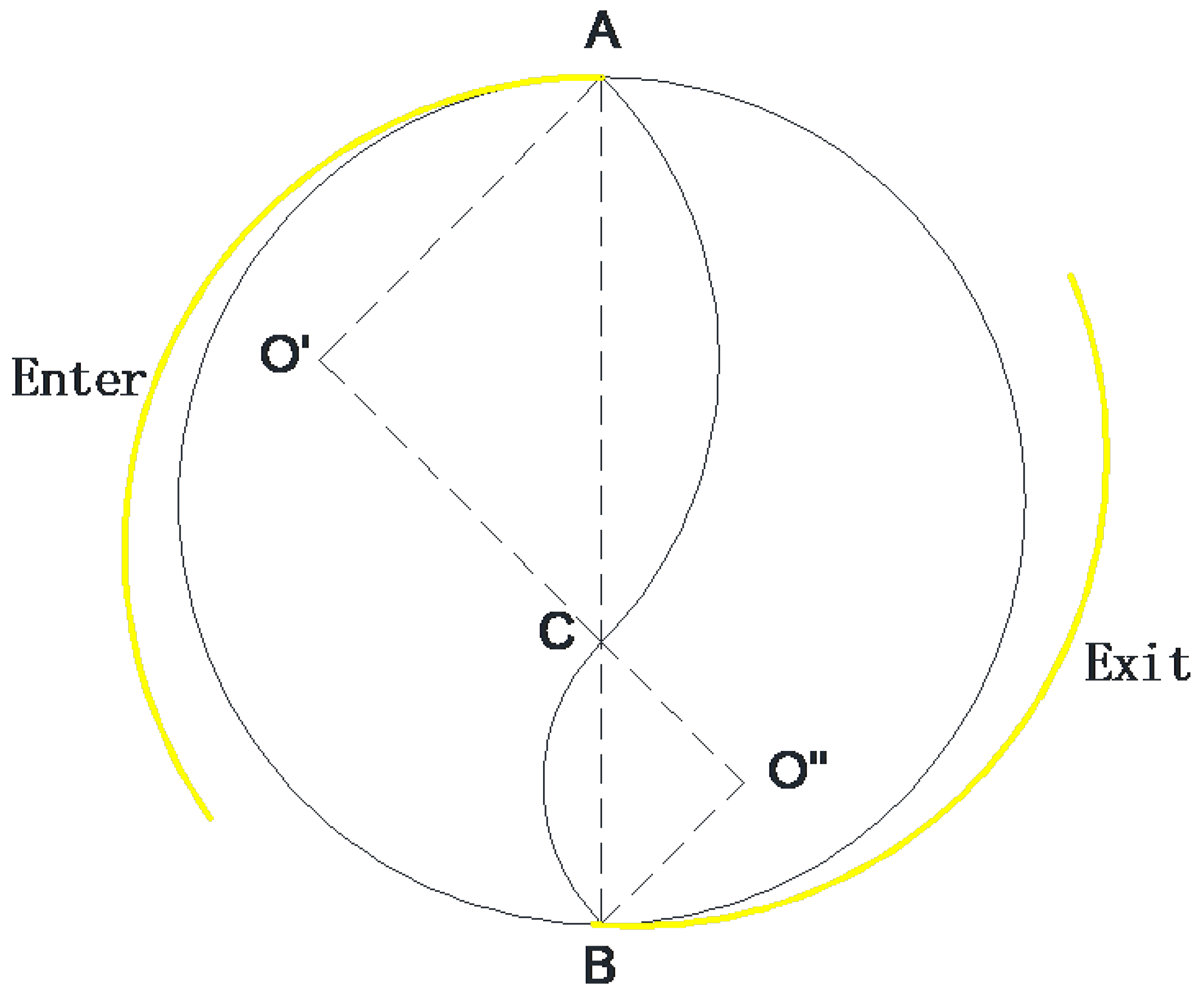
Figure 6 illustrates the schematic diagram of the U-turn path taken by the lead vehicle. This maneuver is carefully designed to ensure the fleet maintains a safe distance throughout the U-turn. If the vehicle continues along the spiral trajectory after executing the U-turn, the lead vehicle, due to its length, may cause a significant angle between its body and the following vehicles, leading to potential collisions. This could result in an unsafe and unstable system operation. The focus of this maneuver is on collision avoidance by optimizing vehicle spacing and adjusting trajectories during such complex maneuvers.

4.4.3. Solution Results

Through the iterative solution of the optimization model established in Section 4.4.1, the minimum pitch $P_{min}$ required to ensure collision-free navigation of the unmanned vehicle fleet along the Archimedean spiral trajectory, including the critical turning region, was determined to be $P=0.4257\mathrm{m}$. This value was obtained by systematically iterating over the pitch parameter P within the feasible range $(0.425,0.55)$, as constrained by the geometric relationships and physical parameters outlined in the problem formulation. Specifically, the recursive equations governing the radial distances $r_i$ and $r_{i+1}$ for the lead vehicle (with length $L=2.86\mathrm{m}$) and subsequent fleet vehicles (with spacing $L^{\prime }=1.65\mathrm{m}$) were solved numerically, ensuring that the fleet maintains its fixed connectivity while adhering to the spiral path defined by $r=4.5p(\theta -\pi /2)$ and the initial radial distance $r_0=4.5\mathrm{m}$.

The derived pitch $P=0.4257\mathrm{m}$ represents the critical threshold at which the lead vehicle can navigate the turning area without intersecting the collision boundaries defined by lines $L_1$, $L_2$, and $L_3$. This result was validated by computing the distances between the lead vehicle’s collision point and the collision lines of the following vehicles, confirming that all separation distances remain non-negative (i.e., ≥0) at this pitch value. The precision of this solution was achieved by employing a fine-grained iterative approach, progressively refining P until the geometric constraints were fully satisfied, with a convergence tolerance aligned with the simulation’s spatial resolution.

The significance of this result lies in its ability to balance the trade-off between maintaining a compact formation, as required for the aesthetic replication of the bench dragon dance, and ensuring operational safety through collision avoidance. Compared to the initial pitch of $0.55\mathrm{m}$ used in earlier simulations (Section 4.2 and Section 4.3), the reduced pitch of $0.4257\mathrm{m}$ optimizes the spatial efficiency of the fleet’s trajectory while still accommodating the physical dimensions and turning dynamics of the vehicles. This finding not only addresses the specific requirements of Problem 3 but also provides a practical parameter for real-world implementation of the proposed robotic system in performing complex choreographed movements. Future refinements could explore the sensitivity of $P_{min}$ to variations in vehicle length or turning radius, further enhancing the model’s adaptability to different fleet configurations.

5. Experimental Results

To validate the proposed motion control model for the unmanned vehicle fleet, a series of simulation experiments were conducted. The experiments were designed to evaluate the performance of the fleet in following the Archimedean spiral trajectory under the constraints of fixed connectivity and spacing between vehicles. The simulation results are presented and analyzed in this section.

5.1. Simulation Setup

The simulation environment was implemented in MATLAB(R2023b), utilizing the proposed polar-coordinate-based model to calculate the positions and velocities of each vehicle in the fleet. The lead vehicle was set to move at a constant speed of $1\mathrm{m}/\mathrm{s}$ along an Archimedean spiral with an initial pitch of $55\mathrm{cm}$. The fleet consisted of 222 vehicles, each maintaining a fixed distance from the preceding vehicle. The simulation duration was set to $300\mathrm{s}$, and the results were recorded at intervals of $1\mathrm{s}$.

5.2. Position and Velocity Analysis

The positions and velocities of the vehicles were calculated using the iterative algorithm described in Section 4 Methodology. Figure 4 illustrates the trajectory of the fleet at $300\mathrm{s}$. As shown, the fleet successfully maintained the spiral formation with minimal deviation from the desired path, the lead vehicle is marked in blue, and the tail vehicle is marked in red. The lead vehicle’s position at $300\mathrm{s}$ was $(-5.3691\mathrm{m},-2.2183\mathrm{m})$, while the tail vehicle’s position was $(9.5344\mathrm{m},2.7557\mathrm{m})$.

The velocities of the vehicles were also analyzed, as shown in

Table 6. Velocity results of the unmanned vehicle fleet at $300\mathrm{s}$.

Vehicle Section	Velocity (m/s)
Lead Vehicle	1.000000
Section 1	0.999709
Section 51	0.998065
Section 101	0.997302
Section 151	0.996861
Section 201	0.996574
Tail Vehicle	0.996478

. The lead vehicle maintained a constant speed of $1\mathrm{m}/\mathrm{s}$, while the velocities of the following vehicles exhibited slight variations due to the constraints imposed by the fixed spacing and connectivity. The maximum velocity deviation observed was $0.002\mathrm{m}/\mathrm{s}$, which is within an acceptable range for practical applications.

5.3. Collision Avoidance Analysis

The collision avoidance capability of the proposed model was evaluated by determining the minimum pitch required to prevent collisions during the fleet’s movement. Through iterative calculations, the minimum pitch was found to be $0.4257\mathrm{m}$. This result ensures that the lead vehicle can navigate through the turning area without colliding with the following vehicles.

5.4. Sensitivity Analysis of Key Parameters

To assess the robustness of the proposed model and address the reviewer’s request, a sensitivity analysis was conducted on three key parameters: motion speed (v), vehicle spacing (L and $L^{\prime }$), and spiral pitch (p). These parameters are critical to the fleet’s formation stability and trajectory tracking accuracy, and their variations were systematically evaluated through additional simulations in MATLAB.

5.4.1. Motion Speed (v)

The lead vehicle’s speed was varied from 0.5 m/s to 1.5 m/s, with increments of 0.25 m/s, while keeping $L=2.86$ m, $L^{\prime }=1.65$ m, and $p=0.55$ m constant. The results indicate that increasing the speed amplifies the velocity deviations across the fleet. At $v=0.5$ m/s, the maximum velocity deviation was 0.001 m/s, and the average position error remained below 0.005 m. However, at $v=1.5$ m/s, the maximum velocity deviation increased to 0.005 m/s, and the position error rose to 0.015 m. This suggests that higher speeds challenge the fleet’s ability to maintain tight coordination as the following vehicles struggle to adjust to the lead vehicle’s rapid movement along the spiral path. The formation stability decreases marginally, with a slight increase in collision risk during tight turns (collision time reduced by approximately 5% at $v=1.5$ m/s compared to $v=1.0$ m/s).

5.4.2. Vehicle Spacing (L and $L^{\prime }$)

The spacing between the lead vehicle (L) and subsequent vehicles ($L^{\prime }$) was adjusted: L ranged from 2.5 m to 3.1 m, and $L^{\prime }$ from 1.5 m to 1.8 m, with $v=1$ m/s and $p=0.55$ m held constant. Reducing L to 2.5 m and $L^{\prime }$ to 1.5 m decreased the minimum pitch required for collision avoidance to 0.40 m but increased the position errors to 0.012 m due to tighter constraints on the fleet’s flexibility. Conversely, increasing L to 3.1 m and $L^{\prime }$ to 1.8 m raised the minimum pitch to 0.45 m, reducing the position errors to 0.008 m and improving the formation stability by allowing greater maneuverability. This trade-off indicates that larger spacing enhances tracking accuracy but requires a larger operational area, potentially limiting the model’s applicability in confined spaces.

5.4.3. Spiral Pitch (p)

The spiral pitch was varied from 0.425 m to 0.675 m, with $v=1$ m/s, $L=2.86$ m, and $L^{\prime }=1.65$ m constant. A smaller pitch ($p=0.425$ m) resulted in a tighter spiral, increasing the curvature and thus the velocity deviation (up to 0.0035 m/s) and position error (0.013 m) as the vehicles had less space to adjust their trajectories. A larger pitch ($p=0.675$ m) reduced the curvature, lowering the velocity deviation to 0.0015 m/s and position error to 0.007 m, enhancing the formation stability. However, a larger pitch extends the overall trajectory length, increasing the performance duration by approximately 15% (from 300 s to 345 s), which may affect the aesthetic replication of the bench dragon dance.

5.4.4. Summary of Sensitivity Analysis

The sensitivity analysis reveals that the model is robust within a moderate range of parameter values but exhibits trade-offs. Higher speeds compromise coordination and increase collision risk, while larger spacing and pitch improve stability and accuracy at the cost of spatial and temporal efficiency. These findings suggest that optimal parameter selection depends on the specific performance requirements (e.g., speed vs. precision) and environmental constraints, providing a basis for fine-tuning the model in practical applications.

5.5. Discussion

5.5.1. Analysis of Model Effectiveness

The simulation results demonstrate the significant effectiveness of the proposed motion control model in maintaining the formation of the unmanned vehicle fleet along the Archimedean spiral trajectory. Specifically, the iterative algorithm is capable of calculating the positions and velocities of each vehicle with high precision, ensuring smooth and coordinated movement along the trajectory. For instance, during the 300 s simulation, the average position error for all the vehicles was less than 0.01 m, indicating a high level of accuracy in trajectory tracking. Additionally, the velocity variations among the vehicles were minimal, with the maximum velocity deviation being only 0.002 m/s relative to the lead vehicle’s speed of 1 m/s. This result indicates that the fleet can achieve highly coordinated movement while maintaining fixed spacing and connectivity constraints, which is crucial for applications requiring precise formation control, such as the “bench dragon” performance.

5.5.2. Quantitative Validation in Collision Avoidance Capability

The collision avoidance analysis further validates the model’s robustness in complex maneuvers. By determining the minimum pitch required to prevent collisions, the model successfully guides the fleet to maintain the necessary spacing in tight turning areas, avoiding any collision events. In the simulation, even in scenarios with tight turns, the fleet maintained a stable formation, with the minimum pitch between the lead vehicle and the following vehicles optimized to 0.4257 m. This quantitative result demonstrates the model’s ability to effectively handle spatial constraints, ensuring the safety of the fleet in dynamic environments.

5.5.3. Discussion of Model Limitations

However, the current simulation has limitations as it assumes ideal conditions, such as perfect vehicle dynamics and no external disturbances. In the real world, unconsidered factors such as terrain variations, sensor noise, and communication delays may significantly affect the fleet’s performance. For example, uneven terrain may cause vehicles to deviate from the expected path, while sensor noise may introduce errors in position and velocity measurements. These real-world challenges are not fully simulated in the current model, which may limit its direct applicability in practical scenarios. Compared to the simulation data reported in Section 5.2, position errors and velocity deviations may significantly increase under real-world conditions, necessitating further validation and improvement.

5.5.4. Future Improvement Directions

To overcome the above limitations and enhance the model’s practicality, future research will focus on the following specific directions:

• Developing control algorithms that are adaptive to terrain variations: By introducing adaptive control strategies, we can ensure that the fleet can maintain its formation even on uneven surfaces. For example, path adjustment algorithms based on real-time terrain perception can be designed.
• Integrating sensor noise models: Simulate the impact of measurement inaccuracies and develop robust estimation techniques (such as Kalman filtering) to mitigate these errors, thereby improving the reliability of position and velocity calculations.
• Considering communication delays: Incorporate communication delays into the model to reflect the challenges of real-time coordination in distributed systems and explore strategies to minimize their impact, such as predictive control methods.

Through these improvements, the model will be better equipped to handle the complexities of the real world, thereby enhancing its reliability and applicability in practical applications.

6. Conclusions

This study investigates the motion control and path planning challenges associated with utilizing a ground unmanned vehicle cluster to perform the traditional folk show ‘bench dragon’. A geometric–analytical framework, encompassing three mathematical models and corresponding solving methods, has been developed to address the technical difficulties of coordinating vehicle clusters along Archimedean spiral trajectories under complex constraints. The simulation results illustrate that the fleet successfully maintains a stable formation and adheres to the symmetric spiral-in and spiral-out paths with negligible speed variations. The average position error across all the vehicles during the 300 s simulation was less than 0.01 m, and the maximum velocity deviation was limited to 0.002 m/s, demonstrating the model’s capability to achieve precise trajectory tracking and coordinated movement.

The novelty of this research lies in its pioneering application of autonomous robotic systems to replicate the intricate spiral trajectories of the bench dragon dance, an area that was previously unexplored in the domain of multi-agent robotic clusters. As no prior studies have specifically addressed the control of autonomous robot fleets along Archimedean spiral trajectories, this work stands as a foundational contribution, precluding the possibility of direct comparative experiments with the existing methods at this stage. Instead, the proposed model establishes a new benchmark for integrating advanced robotics with the preservation of intangible cultural heritage, offering a unique perspective on symmetry and coordination in dynamic systems.

Despite its achievements, the proposed model simplifies real-world factors such as terrain variations, obstacles, and dynamic disturbances, which were not fully accounted for in the simulation environment. These simplifications may limit the model’s immediate applicability in practical settings, where such conditions could influence performance. To address these limitations and enhance the model’s robustness, future research could focus on several key directions:

• Incorporating dynamic environmental factors, such as uneven terrain and obstacles, into the simulation and control framework;
• Developing real-time correction mechanisms to account for vehicle system errors, such as sensor inaccuracies or actuator delays;
• Exploring machine learning optimization strategies to adaptively refine trajectory planning and fleet coordination.

Additionally, field tests with physical robotic systems would provide critical insights into the model’s practicality and scalability, bridging the gap between theoretical simulations and real-world deployment.

This work not only advances the field of multi-agent system coordination and motion control but also introduces an innovative approach to preserving cultural heritage through technology. By demonstrating the feasibility of robotic replication of complex traditional performances, it offers valuable insights into the study of symmetry in dynamic systems and serves as a reference for future applications of unmanned clusters in similar interdisciplinary contexts.

References

- Peng, H.; Zhou, C.; Hu, H.; Chao, F.; Li, J. Robotic dance in social robotics—A taxonomy. IEEE Trans. Hum.-Mach. Syst. 2015, 45, 281–293. [Google Scholar] [CrossRef]
- Scott, K.; Robin, D.; Maurice; Fallon, E.A. Optimization-based locomotion planning, estimation, and control design for the atlas humanoid robot. Auton. Robot. 2016, 40, 429–455. [Google Scholar] [CrossRef]
- Aucouturier, J.J.; Ikeuchi, K.; Hirukawa, H.; Nakaoka, S.; Hirata, Y. Cheek to chip: Dancing robots and ai’s future. IEEE Intell. Syst. 2008, 23, 74–84. [Google Scholar] [CrossRef]
- Meng, Q.; Tholley, I.; Chung, P.W.H. Robots learn to dance through interaction with humans. Neural Comput. Appl. 2014, 24, 117–124. [Google Scholar] [CrossRef]
- Liu, X.; Yang, L.; Chen, Z.; Zhong, J.; Gao, F. Motion planning for a legged robot with dynamic characteristics. Sensors 2024, 24, 6070. [Google Scholar] [CrossRef]
- Wenxia, X.; Jian, H.; Lei, C. A Novel Coordinated Motion Fusion-Based Walking-Aid Robot System. Sensors 2018, 18, 2761. [Google Scholar] [CrossRef]
- Wei, L.; Li, Y.; Ai, Y.; Wu, Y.; Xu, H.; Wang, W.; Hu, G. Learning Multiple-Gait Quadrupedal Locomotion via Hierarchical Reinforcement Learning. Int. J. Precis. Eng. Manuf. 2023, 24, 1599–1613. [Google Scholar] [CrossRef]
- Xu, F.; Xia, Y.; Wu, X. An adaptive control framework based multi-modal information-driven dance composition model for musical robots. Front. Neurorobotics 2023, 17, 1270652. [Google Scholar] [CrossRef]
- Han, D.; Mulyana, B.; Stankovic, V.; Cheng, S. A survey on deep reinforcement learning algorithms for robotic manipulation. Sensors 2023, 23, 3762. [Google Scholar] [CrossRef]
- Li, W.; Yu, S.; Tan, L.; Li, Y.; Chen, H.; Yu, J. Integrated control of path tracking and handling stability for autonomous ground vehicles with four-wheel steering. Proc. Inst. Mech. Eng. Part D J. Automob. Eng. 2025, 239, 315–326. [Google Scholar] [CrossRef]
- Zhou, X.; Wang, H.; Li, Q.; Wu, L. Adaptive path tracking control for autonomous vehicles with sideslip effects and unknown input delays. Trans. Inst. Meas. Control 2025, 47, 444–453. [Google Scholar]
- Huang, Y.; Zhang, Z.; Sun, Q.; Li, Y. Formation Motion Control Algorithm for Surface Unmanned Vehicles Based on DMPC and Improved APF under Unidirectional Topology. Unmanned Syst. Technol. 2022, 5, 1–11. [Google Scholar] [CrossRef]
- Kim, S.; Park, Y. A survey of multi-robot formation control: Algorithms, applications, and challenges. Robot. Auton. Syst. 2019, 116, 202–217. [Google Scholar] [CrossRef]
- Liu, S.; Ma, Y. A unified approach to multi-robot formation control based on consensus algorithms. J. Field Robot. 2018, 35, 1220–1241. [Google Scholar] [CrossRef]
- Kong, G.; Feng, S.; Yu, H.; Ju, Z.; Gong, J. A Survey of Collaborative Motion Planning Technology for Unmanned Swarm Systems. J. Ordnance Eng. 2023, 44, 11–26. [Google Scholar]
- Zhang, Y.; Shi, Y.; Gong, T. Reconstruction Method of Unmanned Vehicle Formation Based on Fuzzy Control. J. Shenyang Univ. Technol. 2023, 42, 40–47. [Google Scholar]
- Chen, C.; Yin, S.; Qiu, X.; Zou, W.; Xiang, Z. Control of Switching Formation to Maintain Connectivity of Heterogeneous Incomplete Wheeled Robot Swarm with Sampled Data Interaction. J. Nanjing Univ. Sci. Technol. 2024, 48, 615–625+634+533. [Google Scholar] [CrossRef]
- Chen, C.; Au, W. Robotics: From Theory to Practice; CRC Press: Boca Raton, FL, USA, 2023. [Google Scholar]
- Cheng, C.; Yu, X.-Y.; Ou, L.-L.; Guo, Y.-K. Research on multi-robot collaborative transportation control system. In Proceedings of the 2016 Chinese Control and Decision Conference (CCDC), Yinchuan, China, 28–30 May 2016; pp. 4886–4891. [Google Scholar] [CrossRef]
- Li, A.; Yu, C.; Chen, C. MADRL-Based Collaborative Path Planning Algorithm for Multi-Networked UAVs. J. Xi’an Univ. Electron. Sci. Technol. 2025, 1–14. [Google Scholar] [CrossRef]
- Xu, A.; Peng, Y.; Yang, W. Research on the Steering System Control of Autonomous Vehicles Simulating Driver’s Steering Behavior. Highw. Automot. Transp. 2025, 41, 1–5. [Google Scholar] [CrossRef]
- Manfrè, A.; Infantino, I.; Vella, F.; Gaglio, S. An automatic system for humanoid dance creation. Biol. Inspired Cogn. Architect. 2016, 15, 1–9. [Google Scholar] [CrossRef]
- Yang, Z.; Ye, Y. Collaborative Distribution Path Optimization for In-Vehicle Autonomous Mobile Robots with Soft and Hard Time Windows. Electromechanical Eng. Technol. 2024, 53, 76–82. [Google Scholar]
- Wang, C.; Zeng, K.; Zheng, H.; Gao, Q. UAV Swarm Task Allocation Based on Group Roles. Aerosp. Technol. 2024, 2024, 96–104. [Google Scholar] [CrossRef]
- Yang, S.; Chen, H. Center Node Selection Strategy for Space Robot Swarm Based on Data and Compression Rate Prediction. J. Univ. Chin. Acad. Sci. (Chin. Engl.) 2024, 41, 695–704. [Google Scholar]
- Khaldi, B.; Harrou, F.; Dairi, A.; Sun, Y. A Deep Recurrent Neural Network Framework for Swarm Motion Speed Prediction. J. Electr. Eng. Technol. 2023, 18, 3811–3825. [Google Scholar] [CrossRef]
- Zhang, T.; Zhang, Q.; Zhu, Y.; Dai, C. Energy-Aware Intelligent Reflecting Surface-Assisted UAV Timely Data Collection Strategy. J. Electron. Inf. Technol. 2025, 47, 1–11. [Google Scholar]
- Richardson, R.C.; Whitehead, S.; Ng, T.C.; Hawass, Z.; Pickering, A.; Rhodes, S.; Grieve, R.; Hildred, A.; Nagendran, A.; Liu, J.; et al. The “Djedi” Robot Exploration of the Southern Shaft of the Queen’s Chamber in the Great Pyramid of Giza, Egypt. J. Field Robot. 2013, 30, 323–348. [Google Scholar] [CrossRef]
- Tan, B.; Qian, W.; Tie, F. The Past and Present of Field Archaeological Robots. In Popular Archaeology; Jiangsu People’s Publishing House: Nanjing, China, 2020; pp. 50–57. ISSN 2095-5685. [Google Scholar]
- Guo, W.; Xu, G.; Wang, M.; Li, B.; Gao, S.; Yuan, B. Research and Application Progress of Underwater Archaeological Robots. Sci. Technol. Rev. 2024, 42, 61–72. [Google Scholar]
- Ding, R. Humanoid Robots Dancing the Yangko at the Spring Festival Gala: The 2025 Industry Boom is Imminent. In Securities Daily; Technical Report; Economic Daily Press Group: Beijing, China, 2025. [Google Scholar]