Abstract
We consider the problem of computed tomography (CT). This ill-posed inverse problem arises when one wishes to investigate the internal structure of an object with a non-invasive and non-destructive technique. This problem is severely ill-conditioned, meaning it has infinite solutions and is extremely sensitive to perturbations in the collected data. This sensitivity produces the well-known semi-convergence phenomenon if iterative methods are used to solve it. In this work, we propose a multigrid approach to mitigate this instability and produce fast, accurate, and stable algorithms starting from unstable ones. We consider, in particular, symmetric Krylov methods, like lsqr, as smoother, and a symmetric projection of the coarse grid operator. However, our approach can be extended to any iterative method. Several numerical examples show the performance of our proposal.
1. Introduction
Computed tomography (CT) is an ill-posed inverse problem extremely relevant in several areas of science, engineering, and cultural heritage preservation. CT is a non-invasive and non-destructive technique used to reconstruct the internal structure of an object. The final result of CT is a map of the absorption coefficients of the object, which can be obtained through the application of the Radon transform. Assume that an X-ray is irradiated at an angle, , through a two-dimensional object. If we represent the absorption coefficient of the scanned object by and assume that f is regular enough, then we can express the Radon transform as follows:
where L is the straight-line path along which the X-ray travels, denotes the line integral along L, summing up the contributions of along that line, and is the total intensity loss of the X-ray beam after passing through the scanned object at an angle . In practice, a CT scanner captures values of for some angles . The fundamental problem in CT imaging is to reconstruct an approximation of , i.e., to recover the internal structure of the object from these measurements.
If we approximate f by a piece-wise constant function on a two-dimensional grid with n elements, we can approximate the integral in (1) by the following:
where denotes the set of indices of the elements of the grid that the X-ray passes through, is the value of the absorption coefficient (that we assumed constant) in the grid element i, and is the length of the path that the X-ray travels in the i-th grid element. Considering a finite set of angles (and, therefore, X-rays) , for , we obtain the following linear system of equations:
We can rewrite the system (2) compactly as follows:
where is usually a rectangular matrix, with , containing the lengths in (2), collects the measurements, and contains the unknown coefficients that we wish to recover. The measurements, , known as the sinogram, are usually corrupted by some errors, and the “exact” ones are usually not available. In practical applications, we only have access to , such that we have the following:
where denotes the Euclidean norm. We will assume that a fairly accurate estimate of is available. The matrix, A, may be ill-conditioned, i.e., its singular values may decay rapidly to zero with no significant gap between consecutive ones. Moreover, the system may have many more unknowns than equations; this may be due to several reasons. For instance, it may be impossible to scan the object from certain angles or one may not want to irradiate it with too much radiations. The latter is a common case when one deals with medical applications. Therefore, the CT inversion is a discrete inverse problem. We refer the interested reader to [1,2] for more details on CT and to [3,4] for more details on ill-posed inverse problems.
Since the linear system of equations
is a discrete ill-posed problem, one needs to regularize it. There are many possible approaches to regularization, in this work, we consider the so-called iterative regularization methods. Iterative methods, like Krylov methods, exhibit the semi-convergence phenomenon [5], i.e., in the first iterations, the iterates approach the desired solution , where denotes the Moore–Penrose pseudo-inverse of A. After a certain, unknown, amount of iterations have been performed, the noise present in is amplified, corrupting the computed solution, and the iterates eventually converge to . The latter is a very poor approximation of , and in most cases, is completely useless. Therefore, regularization is obtained by early stopping the iterations, before the noise is amplified. Determining an effective stopping criterion is still a matter of current research, and an imprudent choice may produce extremely poor reconstructions.
In recent years, Krylov methods have been considered for solving CT imaging problems. In particular, recently, a variation of the GMRES algorithm has been proposed [6]. This method considers an unmatched transpose operator, similar to what has been done in [7] for image deblurring. Algebraic iterative reconstruction methods are possible alternatives to Krylov methods often applied in CT; see [8] and references therein. Several sparsity-promoting algorithms have been proposed in the literature, often in combination with data-driven deep learning methods; see, e.g., [9,10,11]. Concerning multigrid methods, to the best of our knowledge, there are very few proposals, and they consider the multigrid strategy only to accelerate the convergence, solving a Tikhonov regularization model [12], or resorting to a domain decomposition strategy [13,14]. To the best of our knowledge, this is the first time an algebraic multigrid algorithm has been developed to solve the CT problem directly.
In this paper, we propose an iterative regularization multigrid method that stabilizes the convergence of the iterative lsqr method. The latter algorithm is an iterative Krylov method that solves the least-squares problem
As we mentioned above, the solution to the minimization problem (5) is of no interest, and regularization is achieved by early stopping of the iterations. Depending on the problem, the convergence of the lsqr method may be so fast that accurately selecting a stopping iteration may be challenging. Combining this Krylov method with the multigrid approach, with properly selected projection and restriction operators, allows us to construct a more stable and accurate algorithm. This is mainly achieved by exploiting the symmetry of the smoother (lsqr, which solves the symmetric normal equations associated with (5)) and the symmetric Galerkin projection of the coarse operator. Moreover, in our multigrid method, we can simply add the projection into the nonnegative cone to further improve the quality of the reconstruction.
Note that our multigrid method does not resort to Tikhonov regularization as in [12,15], and its aim is not to accelerate the convergence as in [13,14], but is inspired by iterative regularization multigrid methods for image deblurring problems as discussed in [16,17]. Therefore, we obtain a reliable iterative regularization method, robust with respect to the stopping iteration, but with a computational cost usually larger than that of the lsqr method used as the smoother.
2. Multigrid Method
We will now briefly describe how the multigrid method (MGM) works for solving invertible, usually positive definite, linear systems [18]. The main idea of classical MGM is to split into two subspaces. The first one is where the operator, A, is well-conditioned, and the second one is where the operator is ill-conditioned.
It is well-known that iterative methods first reduce the errors in the well-conditioned space and, only in later iterations, solve the problem in the ill-conditioned one. The cost per iteration is usually of the order of the cost of the matrix-vector product with A. Even if matrix A is moderately ill-conditioned, the decrease of the error in the ill-conditioned space may be extremely slow, and, overall, a large number of iterations is required to achieve numerical convergence, making the iterative method computationally unattractive.
On the other hand, direct methods require a fixed amount of operations, regardless of the conditioning of A. However, the cost is usually sensibly higher than the one of a single iteration of iterative methods, i.e., if , then the cost is usually . Moreover, they usually factor the matrix into the product of two or more matrices that are “easier” to handle. However, these factors may not have the same properties as the original matrix. This is particularly of interest if the matrix A is sparse. In this case, even if , it is still possible to store A, however, if the factors are full, they may require too much memory to be stored and handled.
MGM couples the two approaches exploiting the strengths of both iterative and direct methods and overcoming their shortcomings. We define the operators:
where , , , and . The sequence stops when the minimum between and is small enough. The operator projects a vector into a smaller size subspace and, when , we have that , where the superscript T denotes the transposition. If , cannot be the transpose of , due to the difference in the dimensions, but it still represents the adjoint of the operator discretized by . According to the Galerkin approach, we define the following:
The matrices are the projection of the original operator A into smaller subspaces. The choice of such subspaces and, hence, of the projectors and , is crucial for the effectiveness of the MGM. In particular, they have to be the ill-conditioned subspaces of matrices in order to obtain fast convergence. We will discuss later how to choose them to enforce regularization for ill-posed problems.
The MGM is an iterative method. This algorithm is quite involved, therefore, we first describe the two-grid method (TGM).
The TGM, like the MGM, exploits the so-called “error equation”. Let be an approximation of the exact solution . We can write the error as follows:
It is trivial to see that, for the linear system (3), we have the following:
Therefore, an improved approximation of , denoted by , can be obtained by approximately solving the error equation , obtaining , and setting the following:
To compute , one may simply apply a few steps of an iterative method, however, as we discussed above, this would reduce the error only in the well-conditioned space. Reducing the error in the ill-conditioned space may require too much computational work using a simple iterative method. Therefore, in order to obtain a fast solver, we wish to exploit direct methods to tackle the ill-conditioned space. The main drawback of direct methods is the high computational cost. Assuming that projects into a subspace of small dimension such that can be factorized cheaply, then a system of the form can be solved efficiently using a direct method. A single iteration of the TGM goes as follows:
where by , we denote the application of a few steps of an iterative method, like a Krylov method, to the original system (3), with the starting guess .
If n is large, which is usually the case, then may be too large to invert; therefore, to solve the system, one can use the TGM, further projecting the problem. Doing this recursively gives rise to the MGM algorithm. One projects the problem L times until the sizes of are small enough to directly invert it. We refer to each projection as a level. We summarize the computation of a single iteration of MGM in Algorithm 1.
Note that in Algorithm 1 we do not specify explicitly the stopping criterion so that we can later tailor the algorithm to our application of interest, i.e., CT. Also, for , the initial guess is the zero vector. This is because, on lower levels, we are solving the error equation, and one expects the solution to have all vanishing components.
Note that in CT problems, the ill-conditioned subspace resides in the high frequencies. Therefore, if we project into such a subspace to speed up convergence, we risk amplifying the noise, which can destroy the quality of the restored image. On the other hand, for this application, stabilizing instead of accelerating the convergence is more important. Therefore, in the next section, we will choose the grid transfer operators to project the problem in the lower frequencies as done in [16,17] for image deblurring problems. The main difference between image deblurring and CT is that, in image deblurring, matrix A is square and structured (e.g., block Toeplitz with Toeplitz blocks (BTTB), block circulant with circulant blocks (BCCB)), while here, in CT, we consider rectangular sparse matrices, so the methods used for image deblurring cannot be applied.
| Algorithm 1: MGM method |
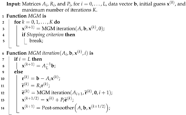 |
3. Our Proposal
We are now in a position to detail our algorithmic proposal.
The first element we wish to describe is the restriction operator, . The prolongation is chosen as . We will assume that the vector is the vectorization of a two-dimensional matrix X, i.e.,
where the operator “vec” orders the entries of X in lexicographical order. We denote the inverse operation by “”. For simplicity of notation, we will assume that , i.e., that X is a square of size . The restriction operator combines two operators. The first, defined by a stencil with , selects the subspace to which the problem is projected; see [19] for further details. The second one is a downsampling operator, which defines the size of the coarser problem. In detail, if s is odd, it is defined as follows:
while, if s is even, it is defined as follows:
Let ∗ denote the convolution operator and ⊗ denote the Kronecker product; then, we define the following:
We can iteratively define by applying the above construction to the lower levels. Namely, if , then we define as in (6) if is odd or as in (7) if is even. Assuming , then we define the following:
We consider four possible choices of M, as follows:
These correspond to different B-spline approximations, where has order i [20]. The first one, i.e., , sums up four adjacent grid elements, while the other ones correspond to different types of averages. We wish to discuss in more detail. Using this restrictor corresponds to summing up the lengths of the ray at a certain angle on each of the four grid elements that are “fused” to get from level i to level ; see Figure 1. Therefore, using this restrictor, intuitively, corresponds to re-discretizing the problem on a coarser grid when we move from level i to level and, in some sense, construct a so-called “geometric” multigrid.
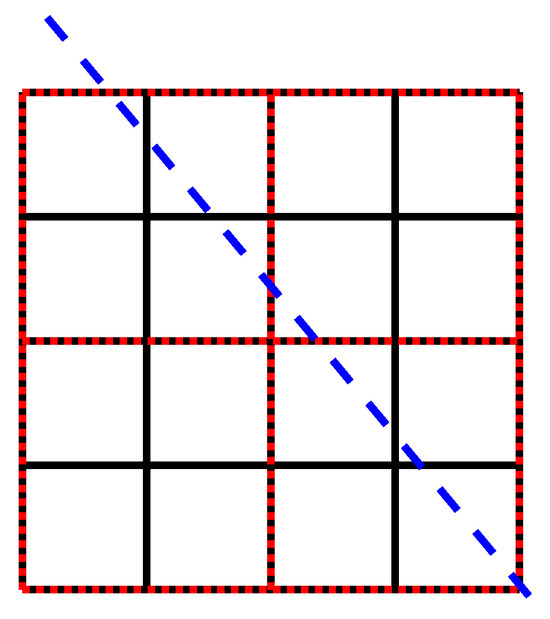
Figure 1.
An X-ray going through an object discretized at two different levels of the MGM. In black is the grid at level i and in red is the one at level . The blue dashed line represents an X-ray going through the object. Each square represents a small portion of the object where we assume the structure to be constant.
Theoretically, the difference between the operators is that each one has a different order, changing the size of the low-frequency subspace, where we project the problem [21]. Furthermore, when the order is even, the operators are symmetric, while the others are not.
As the post-smoother, we use the lsqr algorithm; see [22]. The lsqr method is crucial to our proposal since it can handle rectangular matrices, which is usually the case with CT, and provides a more stable implementation of the mathematically equivalent CGLS [23]. Given an initial guess, , and an initial residual, , this Krylov method, at each iteration, solves the following:
where
The lsqr algorithm uses the Golub–Kahan bidiagonalization algorithm to construct an orthonormal basis of . We will assume that we have access to the matrix or to an accurate approximation of it; see [2,6] for a discussion on non-matching transposes in CT. In the latter case, one may need to use reorthogonalization on the Golub–Kahan algorithm.
Absorption coefficients are always nonnegative, therefore, to ensure that the computed solution satisfies this property, at each iteration, we project the computed solution in the nonnegative cone. This can be simply achieved by setting all the negative values to zero. Projection into the nonnegative cone is often employed in the solution to ill-posed inverse problems since the projection into a convex set is a form of regularization; see, e.g., [24,25,26]. This nonnegative projection is performed after the post-smoother and only at the finest level , because the coarser levels solve the error equations, so they do not have any sign constraints.
Finally, we describe the stopping criterion employed in our algorithm. If we let , then would converge to a solution to the noisy problem (5). As mentioned above, this is not ideal as this solution is usually meaningless. To achieve regularization, we early stop the iterations. We employ the discrepancy principle (DP); see [3]. The DP prescribes that the iterations are stopped as soon as the following condition is met:
where is an upper-bound for the norm of the noise (see (4)) and is a user- defined constant.
The theory of the discrepancy principle states that the parameter has to be greater than one [27]; however, the greater we take it, the earlier it stops the method, so it is common practice to choose a value very close to 1 [28]. To summarize, the novelty of our method stands in the choice of the grid transfer operators, as long as the projection in the nonnegative cone, which is specific to the CT problem. We sum up the computations in Algorithm 2. Note that, since the matrix might be rectangular and may be rank-deficient, we use rather than .
| Algorithm 2: MGM method for CT |
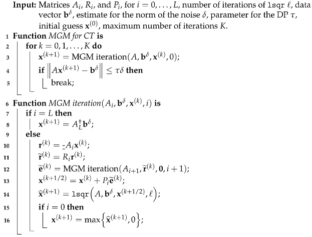 |
4. Numerical Examples
To show the potentiality and performance of our algorithmic proposal, we consider three examples with synthetic data.
Our aim is to show that, coupling MGM with a Krylov method, like lsqr, produces a more stable and more accurate algorithm. Therefore, we compare our approach with the usage of lsqr and the simultaneous iterative reconstruction technique (SIRT), which is a regularized form of a weighted least squares method often used in computed tomography problems [29,30].
We compare the methods in terms of the number of iterations and accuracy. We measure the latter using the relative restoration error defined by the following:
As mentioned above, we stop our method, as well as lsqr and SIRT, with the DP, where we set . Moreover, we set the number of iterations of lsqr to perform at each iteration of MGM to and we set a maximum number of outer iterations, .
The matrix A was explicitly formed using the MATLAB IRTools toolbox [28].
All computations were performed on MATLAB r2021b running on Windows 11 on a laptop with an 11th Gen Intel Core i7 processor with 16 GB of RAM with 15 digits of precision.
- Shepp–Logan (full angles).
In our first example, we consider the Shepp–Logan phantom discretized on a grid of pixels; see Figure 2a. We irradiate the phantom with 362 parallel rays at 180 equispaced angles between 0 and . Therefore, we obtain . This is an ideal case, where we assume that we can irradiate the object with as many rays and from as many angles as we wish. We obtain the noise-free sinogram in Figure 2b. We consider different levels of noise to show the behavior of our method in different scenarios. The noise level is if we have the following:
We set and always consider white Gaussian noise. We report the noise-corrupted sinogram with in Figure 2c. Note that .
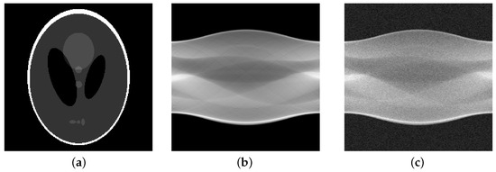
Figure 2.
Shepp–Logan phantom test problem: (a) True image ( pixels), (b) True sinogram ( pixels), (c) Noisy sinogram (10% Gaussian noise).
As mentioned above, we compare our algorithm with lsqr and SIRT. As stated above, we expect the solution to be nonnegative and, therefore, in our method, we project the computed solution into the nonnegative cone at each iteration. To improve its accuracy further, we perform the same projection in the lsqr method ensuring that all the computed solutions are physically meaningful. In all the tests, the SIRT method performed worse than the others, computing not very accurate reconstructions and requiring a large amount of iterations to converge. In Figure 3, we report the evolution of the RRE against the iterations for all considered methods and noise levels. We can observe that semi-convergence is more evident for the lsqr method than for our algorithmic proposal. Regardless of the considered, our method is more stable than lsqr as the RRE increases much slower. We can also observe that the convergence is the most stable when . This is more evident for higher levels of noise. It is clear that, for the lsqr method, if one overestimates the stopping iteration, then the RRE may become extremely large. This is not the case for our MGM methods. In Table 1, we report the RRE obtained at the “optimal” iterations, i.e., the one that minimizes the RRE, and at the DP iteration. In all cases, we can observe that our method is more accurate than the lsqr algorithm, albeit at a generally higher computational cost. However, we would like to stress that the cost per iteration of both lsqr and the MGM is of the same order of magnitude as one matrix-vector product with A and one with , as analyzed in [16]. Since A is extremely sparse, this cost is ; therefore, performing few iterations is computationally extremely cheap. For the noise level, , we report the solutions computed by lsqr and by the MGM with in Figure 4.
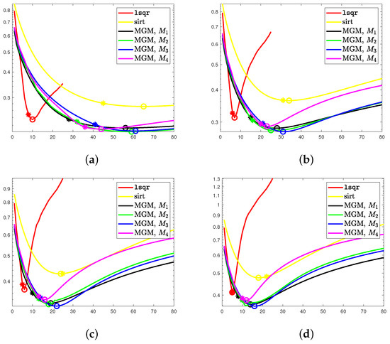
Figure 3.
Shepp–Logan phantom (full angles). Evolution of the RRE against the iteration for each considered noise level. The ∗ marks the discrepancy principle iteration, while ∘ denotes the optimal one. (a) , (b) , (c) , (d) .

Table 1.
Shepp–Logan phantom with full and limited angles. RREs and stopping iterations (in brackets) obtained with lsqr and the MGM for the different choices of in (8).
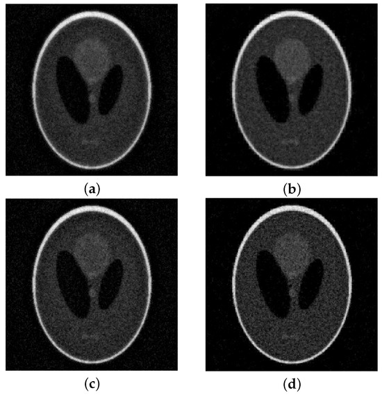
Figure 4.
Shepp–Logan (full angles) with 10% noise. On top of the reconstructions obtained at the DP iteration: (a) lsqr, (b) MGM, . At the bottom, the optimal reconstructions: (c) lsqr, (d) MGM, .
We conclude this example by showing the behavior of our method when we set . We fix , , and we compare the RRE evolution against the iterations of lsqr and MGM with either and , i.e., when we perform two steps of the post-smoother. We show this in Figure 5. We can observe that for , the number of iterations required to reach convergence decreases significantly, even though the cost per iteration is doubled. The resulting method is, however, less stable than the one with , and the obtained RRE is slightly higher. Therefore, in the following, we will set for all examples.
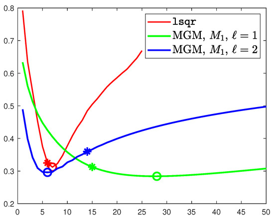
Figure 5.
Evolution of the RRE against the iteration for the multigrid with grid transfer operators of order one. Comparison between 1 and 2 steps of lsqr as the post-smoother. The ∗ marks the discrepancy principle iteration, while ∘ denotes the optimal one.
- Shepp–Logan (limited angles).
Depending on the situation, it may occur that one cannot irradiate an object with as many rays as required. It is, therefore, of high importance to verify how an algorithm performs when fewer data are collected. To this aim, we now consider the same phantom as above, but only half of the angles, i.e., we select 90 equispaced angles between 0 and . This produces a matrix . Note that the number of columns of A is roughly double the number of rows.
As above, we consider four levels of noise, namely and report the evolution of the RRE in Figure 6. We can observe that the obtained results are similar to the ones in the previous case, i.e., our method is more accurate and more stable, albeit requiring more iterations to converge. Moreover, as in the previous case, the highest stability is obtained for . This is confirmed by the results in Table 1. For the noise level , we report the solutions computed by lsqr and by the MGM with in Figure 7. Note that all the operators perform well, improving the stability of lsqr and keeping the same computational cost. However, has the lowest semi-convergence, especially with higher levels of noise and when the problem is strongly underdetermined due to the limited angles used.
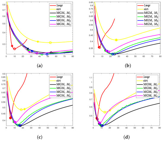
Figure 6.
Shepp–Logan phantom (limited angles). Evolution of the RRE against the iteration for each considered noise level . The * marks the discrepancy principle iteration, while ∘ denotes the optimal one. (a) , (b) , (c) , (d) .
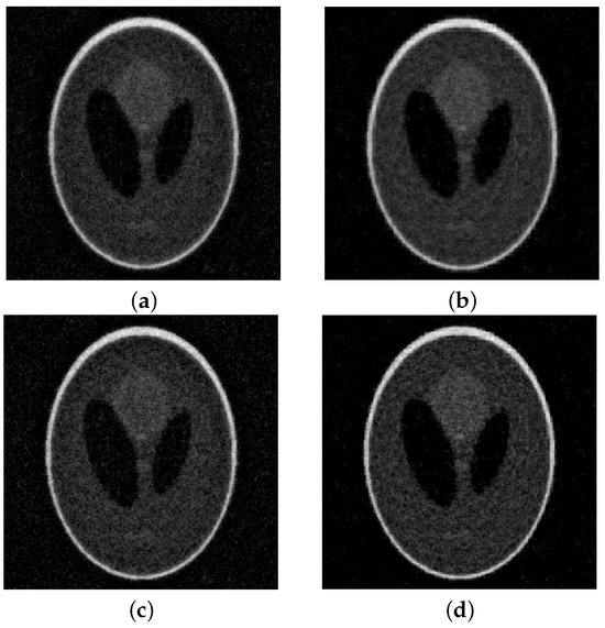
Figure 7.
Shepp–Logan (limited angles) with 10% noise. On top of the reconstructions obtained at the DP iteration: (a) lsqr, (b) MGM, . At the bottom the optimal reconstructions: (c) lsqr, (d) MGM, .
- MRI image.
Finally, we consider a more realistic image. This is a slice taken from an anisotropic 3D MRI volume that simulates the scan of a human brain present in the MRI dataset in MATLAB. In this case, the image is composed of pixels; see Figure 8. We irradiate the image with 181 parallel rays at 90 equispaced angles between 0 and . This produces a matrix . We corrupt the data with white Gaussian noise, resulting in the sinogram shown in Figure 8b.
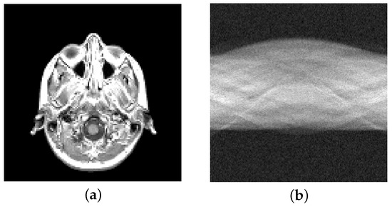
Figure 8.
MRI image test problem: (a) True image ( pixels), (b) noisy sinogram (5% Gaussian noise).
We report the evolution of the RRE against the iterations in Figure 9. We can observe that the results are very close to the ones obtained for the Shepp–Logan phantom. In particular, gives more stable convergence, while higher-order projectors provide slightly better reconstructions. This can also be seen from the results reported in Table 2 and Figure 10. The latter shows the computed solutions by the MGM using and , each stopped at the discrepancy principle iteration.
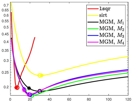
Figure 9.
MRI image. Evolution of the RRE against the iteration with 5% Gaussian noise. The ∗ marks the discrepancy principle iteration, while ∘ denotes the optimal one.
Table 2.
MRI image. RREs and stopping iterations (in brackets) obtained with lsqr and the MGM for the different choices of in (8) with 5% noise.
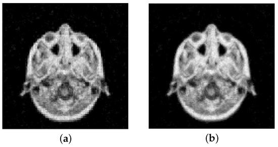
Figure 10.
MRI test image with 5% noise. Reconstructions obtained at the DP iteration: (a) MGM, , (b) MGM, .
5. Conclusions
In this paper, we proposed a multigrid method for solving the CT problem. The proposed method is obtained using the lsqr algorithm as the post-smoother. We showed that combining a Krylov method with the multigrid approach can improve the accuracy of the algorithm and greatly improve its stability. This latter property is of extreme interest as it mitigates the semi-convergence phenomenon and simplifies the task of selecting an appropriate stopping criterion, allowing for greater confidence in consistently obtaining good reconstructions, even when the problem is highly underdetermined and ill-conditioned due to high levels of noise. Several computed examples showed that our method is stable and produces satisfactory results. Future work will include extending this approach to three-dimensional CT applications, with the aid of multilinear linear algebra techniques, applying it to real datasets, and combining it with variational methods.
Author Contributions
Conceptualization, A.B. and M.D.; Implementation, A.B. and M.R.; writing—original draft preparation, A.B., M.D. and M.R.; writing—review and editing, A.B., M.D. and M.R.; Validation, A.B., M.D. and M.R. These authors made equal contributions to this work. All authors have reviewed and approved the final version of the manuscript.
Funding
The authors are members of the GNCS group of INdAM and are partially supported by INdAM-GNCS 2024 Project “Tecniche numeriche per problemi di grandi dimensioni” (CUP_ E53C24001950001). A.B. is partially supported by the PRIN 2022 PNRR project no. P2022PMEN2 financed by the European Union—NextGenerationEU and by the Italian Ministry of University and Research (MUR). A. B. and M. D. are partially supported by the PRIN 2022 project “Inverse Problems in the Imaging Sciences (IPIS)” (2022ANC8HL) financed by the European Union—NextGenerationEU and by the Italian Ministry of University and Research (MUR). A.B.’s work is partially funded by Fondazione di Sardegna, Progetto biennale bando 2021, and “Computational Methods and Networks in Civil Engineering (COMANCHE)”.
Data Availability Statement
Data are contained within the article.
Conflicts of Interest
The authors declare no conflicts of interest. The funders had no role in the design of the study; in the collection, analysis, or interpretation of data; in the writing of the manuscript; or in the decision to publish the results.
References
- Buzug, T.M. Computed tomography. In Springer Handbook of Medical Technology; Springer: Berlin/Heidelberg, Germany, 2011; pp. 311–342. [Google Scholar]
- Hansen, P.C.; Jørgensen, J.; Lionheart, W.R.B. Computed Tomography: Algorithms, Insight, and Just Enough Theory; Society for Industrial and Applied Mathematics: Philadelphia, PA, USA, 2021. [Google Scholar]
- Engl, H.W.; Hanke, M.; Neubauer, A. Regularization of Inverse Problems; Springer Science & Business Media: Berlin/Heidelberg, Germany, 1996; Volume 375. [Google Scholar]
- Hansen, P.C. Rank-Deficient and Discrete Ill-Posed Problems: Numerical Aspects of Linear Inversion; SIAM: Philadelphia, PA, USA, 1998. [Google Scholar]
- Hanke, M. Conjugate Gradient Type Methods for Ill-Posed Problems; Chapman and Hall/CRC: Boca Raton, FL, USA, 2017. [Google Scholar]
- Hansen, P.C.; Hayami, K.; Morikuni, K. GMRES methods for tomographic reconstruction with an unmatched back projector. J. Comput. Appl. Math. 2022, 413, 114352. [Google Scholar] [CrossRef]
- Donatelli, M.; Martin, D.; Reichel, L. Arnoldi methods for image deblurring with anti-reflective boundary conditions. Appl. Math. Comput. 2015, 253, 135–150. [Google Scholar] [CrossRef]
- Dong, Y.; Hansen, P.C.; Hochstenbach, M.E.; Brogaard Riis, N.A. Fixing nonconvergence of algebraic iterative reconstruction with an unmatched backprojector. SIAM J. Sci. Comput. 2019, 41, A1822–A1839. [Google Scholar]
- Rantala, M.; Vanska, S.; Jarvenpaa, S.; Kalke, M.; Lassas, M.; Moberg, J.; Siltanen, S. Wavelet-based reconstruction for limited-angle X-ray tomography. IEEE Trans. Med. Imaging 2006, 25, 210–217. [Google Scholar] [PubMed]
- Bubba, T.A.; Kutyniok, G.; Lassas, M.; März, M.; Samek, W.; Siltanen, S.; Srinivasan, V. Learning the invisible: A hybrid deep learning-shearlet framework for limited angle computed tomography. Inverse Probl. 2019, 35, 064002. [Google Scholar]
- Xiang, J.; Dong, Y.; Yang, Y. FISTA-Net: Learning a Fast Iterative Shrinkage Thresholding Network for Inverse Problems in Imaging. IEEE Trans. Med. Imaging 2021, 40, 1329–1339. [Google Scholar] [CrossRef] [PubMed]
- Bolten, M.; MacLachlan, S.P.; Kilmer, M.E. Multigrid preconditioning for regularized least-squares problems. arXiv 2023, arXiv:2306.11067. [Google Scholar] [CrossRef]
- Marlevi, D.; Kohr, H.; Buurlage, J.W.; Gao, B.; Batenburg, K.J.; Colarieti-Tosti, M. Multigrid reconstruction in tomographic imaging. IEEE Trans. Radiat. Plasma Med. Sci. 2019, 4, 300–310. [Google Scholar] [CrossRef]
- Zhang, Z.; Chen, K.; Tang, K.; Duan, Y. Fast multi-grid methods for minimizing curvature energies. IEEE Trans. Image Process. 2023, 32, 1716–1731. [Google Scholar]
- Donatelli, M. A multigrid for image deblurring with Tikhonov regularization. Numer. Linear Algebra Appl. 2005, 12, 715–729. [Google Scholar]
- Donatelli, M.; Serra-Capizzano, S. On the regularizing power of multigrid-type algorithms. SIAM J. Sci. Comput. 2006, 27, 2053–2076. [Google Scholar]
- Buccini, A.; Donatelli, M. A multigrid frame based method for image deblurring. Electron. Trans. Numer. Anal. 2020, 53, 283–312. [Google Scholar]
- Briggs, W.L.; Henson, V.E.; McCormick, S.F. A Multigrid Tutorial; SIAM: Philadelphia, PA, USA, 2000. [Google Scholar]
- Bolten, M.; Donatelli, M.; Huckle, T. Analysis of smoothed aggregation multigrid methods based on Toeplitz matrices. Electron. Trans. Numer. Anal. 2015, 44, 25–52. [Google Scholar]
- Donatelli, M. An algebraic generalization of local Fourier analysis for grid transfer operators in multigrid based on Toeplitz matrices. Numer. Linear Algebra Appl. 2010, 17, 179–197. [Google Scholar]
- Donatelli, M.; Serra-Capizzano, S. Filter factor analysis of an iterative multilevel regularizing method. Electron. Trans. Numer. Anal. 2007, 29, 163–177. [Google Scholar]
- Golub, G.H.; Van Loan, C.F. Matrix Computations; JHU Press: Baltimore, MD, USA, 2013. [Google Scholar]
- Björck, r.; Elfving, T.; Strakos, Z. Stability of Conjugate Gradient and Lanczos Methods for Linear Least Squares Problems. SIAM J. Matrix Anal. Appl. 1998, 19, 720–736. [Google Scholar] [CrossRef]
- Bai, Z.Z.; Buccini, A.; Hayami, K.; Reichel, L.; Yin, J.F.; Zheng, N. Modulus-based iterative methods for constrained Tikhonov regularization. J. Comput. Appl. Math. 2017, 319, 1–13. [Google Scholar] [CrossRef]
- Gazzola, S. Flexible CGLS for box-constrained linear least squares problems. In Proceedings of the 2021 21st International Conference on Computational Science and Its Applications (ICCSA), Cagliari, Italy, 13–16 September 2021; pp. 133–138. [Google Scholar] [CrossRef]
- Nagy, J.G.; Strakos, Z. Enforcing nonnegativity in image reconstruction algorithms. In Proceedings of the Mathematical Modeling, Estimation, and Imaging, San Diego, CA, USA, 31 July–1 August 2000; Volume 4121, pp. 182–190. [Google Scholar]
- Groetsch, C. The Theory of Tikhonov Regularization for Fredholm Equations of the First Kind; Chapman & Hall/CRC Research Notes in Mathematics Series; Pitman Advanced Pub. Program: London, UK, 1984. [Google Scholar]
- Gazzola, S.; Hansen, P.C.; Nagy, J.G. IR Tools: A MATLAB package of iterative regularization methods and large-scale test problems. Numer. Algorithms 2019, 81, 773–811. [Google Scholar] [CrossRef]
- Elfving, T.; Hansen, P.C.; Nikazad, T. Semiconvergence and Relaxation Parameters for Projected SIRT Algorithms. SIAM J. Sci. Comput. 2012, 34, A2000–A2017. [Google Scholar] [CrossRef]
- Hansen, P.C.; Saxild-Hansen, M. AIR Tools—A MATLAB package of algebraic iterative reconstruction methods. J. Comput. Appl. Math. 2012, 236, 2167–2178. [Google Scholar] [CrossRef]
Disclaimer/Publisher’s Note: The statements, opinions and data contained in all publications are solely those of the individual author(s) and contributor(s) and not of MDPI and/or the editor(s). MDPI and/or the editor(s) disclaim responsibility for any injury to people or property resulting from any ideas, methods, instructions or products referred to in the content. |
© 2025 by the authors. Licensee MDPI, Basel, Switzerland. This article is an open access article distributed under the terms and conditions of the Creative Commons Attribution (CC BY) license (https://creativecommons.org/licenses/by/4.0/).