1. Introduction
Fractional calculus is a branch of mathematics that generalizes differentiation and integration to non-integer orders. Currently, fractional calculus is rapidly evolving within applied mathematics, physics, engineering, and most scientific fields [
1,
2,
3,
4]. This growth has been driven by fractional calculus’s unique capability to model complex phenomena, exhibit memory dependence, and demonstrate non-local behavior, which appear in various systems and may not be captured by traditional integer-order models [
5,
6,
7,
8]. The fact that a substantial amount of high-impact research has emerged demonstrates the numerous applications and practical significance of fractional calculus [
9,
10].
Various studies have demonstrated fractional calculus’s ability to analyze complex dynamical systems, including chaotic systems with multiple coexisting attractors, fractional-order circuits, and encryption mechanisms. In summary, these studies highlight fractional calculus’s ability to enhance system adaptability, detect dynamic features, and model intricate behaviors across various fields [
11,
12,
13,
14,
15].
The Caputo fractional derivative is one of the most popular variants since it incorporates memory effects and hereditary properties in an appropriate way that aligns with realistic modeling in complex systems [
16,
17]. The Caputo derivative offers advantages over other derivatives in terms of computational simplicity, accuracy, smoother solution regularity, and better convergence properties. Furthermore, it is well suited for the analysis of initial-value problems in physical and biological systems, where the initial conditions generally involve standard integer-order derivatives [
18,
19,
20]. These features make the Caputo fractional derivative highly suitable for analyzing dynamic behavioral systems and modeling fractional-order epidemiology, offering a valuable tool for simulating complex disease behaviors often overlooked by traditional models [
21,
22].
Recently, fractional calculus has played a crucial role in integrating numerical schemes with approximate solutions for complex systems. Numerical schemes, such as finite difference, finite element, and spectral methods, have been combined with fractional derivatives to efficiently solve problems in materials science, control systems, and fluid dynamics [
23,
24,
25,
26,
27]. Additionally, it has been successfully applied to the simulation of anomalous diffusion processes, wave propagation in heterogeneous media, and financial modeling, where traditional methods struggle to capture underlying complexities [
28,
29,
30,
31]. By combining numerical techniques with approximate fractional solutions, these methods enhance the accuracy and efficiency of solving real-world problems exhibiting memory effects and long-range interactions.
Numerous analytical methods have been used to solve fractional systems, each with strengths and applications. We highlight the construction of approximate solutions to the model (
2) using a numerical approach to NCFD in terms of the fractional operator paradigm, as presented in [
32]. This is particularly suitable for handling the complexities brought by fractional dynamics, and it provides a good and accurate approximation of the system’s behavior over time. We used this approach due to its ability to handle the complexity of fractional-order systems, e.g., memory effects and long-range dependence, which are of utmost importance in capturing the chaotic behavior of the inverted Rössler system. Our preferred numerical approach ensures convergence and stability, as well as its ability to handle the complexity of the system’s dynamics, making it a very efficient tool in chaotic detection.
The Homotopy Perturbation Method (HPM) [
33,
34,
35,
36,
37] is a semi-analytic technique introduced to deal with linear and nonlinear problems. It is considered a complete and accurate method. To develop perturbation techniques, which need a small parameter in the equation, the main idea behind this method is to build a homotopy that includes the parameter q. As q transitions from 0 to 1, the deformation process occurs, accompanied by the initial solution being deformed into the original solution of the equation. The noticeable aspect is that we can guess the initial approximate solution by leveraging the given conditions, which are a basic requirement for the method to work. Furthermore, the HPM breaks down the nonlinear terms into special polynomials, which are called He’s polynomials [
38,
39]; the final solution appears in a series form. Many modifications of the method have been used and discussed by researchers, revealing a significant improvement in analytical solutions. The He–Laplace method [
40,
41] uses the approach of combining analytical methods with integral transforms [
42,
43,
44,
45,
46]. It is therefore a hybrid analytical method, combining the merits of the Homotopy Perturbation method, the Laplace transform, and He’s polynomials. It is used to handle differential equations more efficiently by reducing them to algebraic forms that we can easily solve. The He–Laplace method results in fast-converging approximate or exact solutions with low computational cost, leading to a systematic approach. Moreover, the He–Laplace method has turned out to be an effective instrument for intricate fractional systems. These results contribute to enhancing the reach and precision of solution methods for fractional calculus and applied mathematics.
The classical Rössler system consists of three interconnected nonlinear ordinary differential equations (ODEs) that model a chaotic dynamical system. Since its introduction by R¨ossler in the 1970s, it has remained a standard example in chaos theory [
47]. Symmetric inversion represents a deviation from the classical Rössler system. This variation significantly impacts its behavior and stability. These chaotic systems are studied to analyze their stability, identify their dynamic properties, and understand how chaos influences real-world systems. Researchers also seek control strategies for these systems and explore their potential practical applications in scientific fields. The equations in an inverted Rössler system are given by [
48]
X, Y, and Z represent the dimensions, while A, B, and C are referred to as control parameters. We present two methods for the numerical approximation of the results: one based on the Caputo fractional derivative and another based on the H-LM to find semi-analytical solutions. Caputo-type derivatives offer significant advantages in modeling the system, including the ability to describe memory effects with flexible parameters due to the fractional order, maintaining the smoothness of the solutions, and enabling more precise modeling of chaotic dynamics. The above advantages make this approach based on Caputo derivatives much more suitable for complex systems.
where
,
, and
, with initial conditions
.
The fractional-order inverted Rössler system, which is represented by Equation (
2), generalizes the classical chaotic model by adding memory effects in the form of Caputo fractional derivatives. The addition of memory effects allows a better description of sophisticated dynamical behaviors, in which the system states are not only dependent on the current conditions but also on their history. The fractional model works excellently in capturing long-range dependencies and abnormal diffusion phenomena and thus has practical applications in physics, engineering, and biological systems. Researchers can adjust the order of the fraction so that the system’s reaction to outside influences is maximized, and its prediction capability is enhanced where traditional integer-order models fail to detect subtle dynamical patterns.
This paper presents two advanced numerical approximation methods for the fractional system, including the Caputo derivative of the inverted symmetric Rössler system. These techniques offer distinct advantages in the detailed analysis of the system’s complex dynamics. The H-LM is highly effective due to its rapid convergence and high computational efficiency, making it well suited for obtaining approximate solutions with minimal computational resources. In contrast, the Caputo fractional derivative method reveals the system’s chaotic behavior and provides chaotic solutions, making it capable of analyzing complex dynamics such as symmetric attractors and chaos detection. A detailed comparison of the two techniques is conducted, considering their precision, computational speed, advantages, and disadvantages. A performance comparison between the H-LM and the Caputo method provides an overview of the applicability and relevance of both methods in chaotic systems. The results are expected to be valuable for future applications of these methods, particularly in systems with sensitive initial conditions and complex strange attractor structures.
Conventional numerical methods, such as the RK4 method and the Adams–Bashforth–Moulton method, have been widely applied to study chaotic systems. They are principally designed for integer-order systems and are not able to represent the memory effects and long-range correlations of fractional-order dynamics. The RK4 method excels in solving ordinary differential equations but is less effective when dealing with fractional derivatives. Similarly, even though predictor-corrector schemes like Adams–Bashforth–Moulton (ABM) are sufficient in terms of accuracy, they are time-consuming and may not preserve chaotic system dynamics. Alternatively, the NCFD scheme is an appropriately designed scheme with numerical stability that also presents an exact chaotic dynamics description in fractional-order systems. Beyond this, the H-LM presents an analytically stable scheme that includes stability and efficiency advantages and can be suitable for fractional chaotic systems. Surpassing the limitations of classical methods, the schemes represent superior tools with which to investigate and model complicated dynamical phenomena.
In this work, we verify the efficacy of two hybrid schemes—the numerical scheme for the Caputo fractional derivative (NCFD) and the He–Laplace Method (H-LM)—in investigating and solving fractional-order chaotic systems. The two methods mainly deviate from and surpass traditional techniques, the latter of which is highly vulnerable to numerical instability or computational complexity. The NCFD method produces extremely high-accuracy numerical solutions, indeed embracing the intricate chaotic dynamics of the fractional-order inverted Rössler system. In contrast, the H-LM offers a quick analytical method that produces accurate and stable solutions with low computational complexity. Combining these two complementary approaches, the current research bridges the numerical accuracy gap with analytical insight and provides a broader understanding of chaotic fractional-order systems. The introduced schemes successfully determine and describe chaotic attractors and have the capacity to model a large class of fractional-order complex systems. These innovations provide new possibilities for scientists and engineers to perform more rigorous simulations and control operations in various applications in science and engineering.
3. Numerical Approach to NCFD
In this section, we discuss the development of the approximate solutions for the model (
2) using an efficient numerical approach in the framework of the fractional operator, as described in [
32]. We consider this method because it allows us to address the complexities arising from fractional dynamics, providing a robust approximation of the system’s behavior over time. Herein, we summarize the results and key observations of the model, focusing on the stability, convergence, and accuracy of the solutions by varying different parameters. The outcomes show the efficiency of the numerical method in capturing the intricate dynamics of the model with high precision.
Finite difference discretization (
):
Lagrange interpolation approximation:
where the Caputo fractional operators and
satisfy the Lipschitz condition as follows:
where
is a Lipschitz constant. By applying (8), we have
where
represents the fractional-order integral operator and the Caputo operator is indicated by the corresponding operators in each case.
Over
, with a constant time step length
during simulation)
, where
, suppose that
is the approximation of
at
for
. The finite difference method for the initial value problem (8) yields the following numerical approach for the underlying operators:
The method is very important, as it handles the intricacies introduced by fractional dynamics with high accuracy. Provides appropriate and stable approximations in the time variation of the system’s behavior. Computationally, it is efficient; hence, this method can accommodate long-term simulations. Moreover, its convergence properties ensure that the results remain reliable under various parameter settings. These advantages confirm the ability of the method to capture intricate model behaviors, thereby proving its effectiveness in providing robust insights into system dynamics.
4. Application of the NCFD to the Inverted Rössler System
This section presents a comprehensive analysis of a system of equations under different initial conditions, fractional orders, and time parameters. We explore the system’s behavior, stability, and the impact of fractional calculus on its dynamics.
Table 1,
Table 2 and
Table 3 provide a summary of the step-by-step analysis of the solutions of a system of equations for different initial conditions and parameters.
Table 1 and
Table 2 consider the system with the initial conditions
and
, respectively, both with
and
. Several step sizes are employed, and one can see in the tables that the solutions converge as the step size decreases. This is an indication of the stability and correctness of the numerical methods being employed. The RK4 method is employed as the benchmark solution against which the accuracy of smaller step sizes is evaluated.
Table 3 presents another example where
and
, with
X,
Y, and
Z. This table shows the behavior of the system over a longer period of time and therefore provides further insight into the numerical accuracy and stability of the system. Together, these tables demonstrate that numerical methods can be very potent in solving complex systems and typically yield great insight into science and engineering for practical applications. Smaller
improves accuracy but increases cost, while larger
risks instability in NCFD simulations.
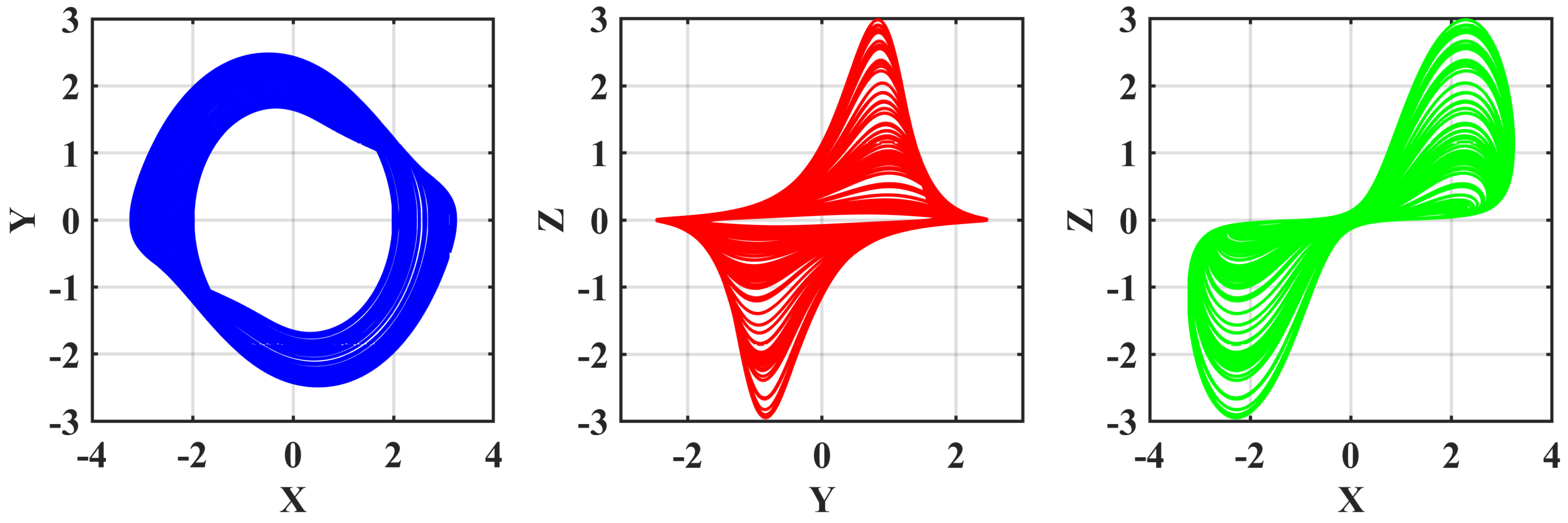
The plots in
Figure 1,
Figure 2,
Figure 3 and
Figure 4 show three different perspectives of system (1) for
,
,
, and 1, with parameters
and initial conditions
. Each group of graphs for a given value of
describes how the system evolves with
and examines its sensitivity to changes in fractional orders. That is, as
, the system’s orbits become clearer, indicating a transition to classical dynamics. These plots effectively illustrate the impact of fractional calculus on system dynamics and show the complex behavior exhibited by systems under different fractional orders. The choice of graphs is not arbitrary but a deliberate attempt to expose the strange features of fractional systems. The graphs provide an integrated view of the impact of fractional orders on system dynamics, filling the gap between application and theory. By illustrating the sensitivity of the system with respect to
α, the plots show the flexibility and richness of fractional calculus, making it an important tool for modeling and analyzing sophisticated systems. This information has extensive applications in science and engineering, offering new ways to study and manipulate systems with memory and non-locality. All the computations were performed using MATLAB R2024a (MathWorks, Inc., Natick, MA, USA).
7. Numerical Method Accuracy
In this section, we compare the accuracy of various numerical methods for solving the system with
.
Table 7 and
Table 8 compare the NCFD method for different step sizes (
and
), the RK4 method for
, and the H-LM, providing insights into the convergence and precision of the methods.
In this section, we present the precision of various numerical schemes applied to the system when
.
Table 7 and
Table 8 give a detailed comparison of the NCFD method for different step sizes (
and
), the RK4 method with a high-precision step size of
, and the H-LM using the first few terms. A comparison of this type is instructive for analyzing the convergence behavior and relative accuracy of the methods, highlighting their weaknesses and strengths in approximating the system dynamics of the three variables (
X,
Y, and
Z).
Table 9 evaluates the accuracy of the H-LM and the NCFD method against the ABM method for
. The results indicate that the H-LM exhibits a small error margin when compared to high-precision ABM solutions (
), testifying to its reliability. The versions of ABM with different step sizes equally highlight the importance of numerical resolution, with finer steps yielding better results. These results validate the H-LM’s ability to solve fractional-order chaotic systems with competitive precision.
To better show the advantages, disadvantages, and range of applications of these methods, we highlight their key characteristics. The advantages of the NCFD method include high numerical accuracy and the ability to capture complex chaotic dynamics, but its main disadvantage is its higher computational cost. The H-LM offers simplicity, stability, and analytic insight but may be limited when dealing with very stiff systems. Both methods are applicable to various fractional-order models in science and engineering, particularly in the analysis of complex and chaotic systems.


 ,
, 


