An Improved Set-Valued Observer and Probability Density Function-Based Self-Organizing Neural Networks for Early Fault Diagnosis in Wind Energy Conversion Systems

Abstract

Fault diagnosis is crucial for ensuring the reliability and safety of wind energy conversion systems (WECSs). However, existing methods are often specific to components or specific types of wind turbines and face challenges, such as difficulty in threshold setting and low accuracy in diagnosing faults at early stages. To address these challenges, this paper proposes a novel fault diagnosis method based on self-organizing neural networks (SONNs) and probability density functions (PDFs). First, an improved set-valued observer (ISVO) is designed to accurately estimate the states of WECSs, considering the time delay and unknown nonlinearity of overall model. Then, the PDF is derived by fitting the estimation error data to characterize three common multiplicative faults of the pitch system actuators. Two types of SONNs are developed to cluster the parameter sets of the PDF. Finally, the PDFs of the estimation error are reconstructed based on the clustering results, thereby designing fault diagnosis strategies that enable a rapid and highly accurate diagnosis of early-stage faults. Simulation results demonstrate that the proposed strategies achieved an early fault diagnosis accuracy rate of over 90%, with the fastest diagnosis time being approximately 0.11 s. Under the same fault conditions, the diagnosis time is 1 s faster than that of a k-means-based fault diagnosis strategy. This study provides a threshold-free, high-accuracy, and rapid fault diagnosis strategy for early fault diagnosis in WECS. By combining neural networks, the proposed method addresses the issue of threshold dependency in fault diagnosis, with potential applications in improving the reliability and safety of wind power generation.

1. Introduction

Wind energy has been widely recognized as one of the most cost-effective and rapidly expanding sources of renewable clean power [1]. The evolution of modern WECS has seen a trend toward large-capacity single machines with automatic operation and unmanned functionality. Over time, the deployment of WECSs has expanded to include deep-sea and high-altitude areas, driven by the need for more efficient and widespread energy generation. However, these advancements have also introduced challenges due to harsh environmental conditions, necessitating stricter requirements for WECS design, layout, fault diagnosis, and fault-tolerant operation. Early research into wind turbine fault diagnosis was categorized by Gao et al. [2] into four distinct methods: model-based methods, signal-based methods, knowledge-based methods, and hybrid methods that combine the three. This foundational work provided a comprehensive literature analysis that set the stage for subsequent research. Building on this, Rezamand et al. [3] later classified fault detection and diagnosis (FDD) into model-based, data-driven, and knowledge-based approaches, further refining the understanding of fault diagnosis methodologies. Zhao [4] contributed to this field by classifying fault detection (FD) of WECS into two categories: methods for the component part and methods for the overall model. This classification underscored the importance of focusing on specific components or different types of wind turbines, such as blade pitches [5], doubly fed induction generators [6,7], and permanent magnet synchronous generators [8]. In more recent studies, Mansouri et al. [9,10] utilized Gaussian process regression (GPR) for feature extraction and developed a fault classifier based on a multi-class random forest (RF) to identify specific faults in IGBTs within WECSs. Their work demonstrated high accuracy and good performance in fault detection. Following this, Fezai et al. [11] proposed a reduced GPR-based RF fault detection strategy, while Mansouri et al. [12] developed an intervalized GPR-based RF fault detection strategy. These strategies showed satisfactory performance compared to traditional methods like principal component analysis (PCA), support vector machine (SVM), decision tree (DT), naive Bayes (NB), discriminant analysis (DA), and k-nearest neighbor (KNN). Hussain et al. [13] summarized 130 research papers on condition monitoring and fault diagnosis of wind turbines, highlighting that data-based fault diagnosis methods were currently the main focus of research; clustering and k-means were the primary techniques for outlier detection; and 12% of the articles addressed non-specific component faults. Despite these advancements, many studies have focused on component faults in WECS, often neglecting the interactions between components and the effects of component faults on the overall system. This limitation has prompted the need for more comprehensive mathematical models that account for the complexity of WECS, including nonlinearities and time delays. Such models would facilitate a deeper understanding of the interactions between components and the impact of component faults on the system, thereby enhancing the research and application of WECS fault diagnosis.

The research on observer-based fault detection for unknown or nonlinear systems highlights several key approaches and their respective contributions and limitations. Zhang et al. [14] proposed a recursive fault detection observer for nonlinear systems experiencing mismatched nonlinear faults, utilizing a predetermined non-negative function related to output estimation accuracy to establish a tight detection threshold. Pujol-Vazquez et al. [15] developed dual observers capable of estimating upper and lower bounds of errors, along with fault detection and classification strategies. However, their approach faced significant limitations, including the lack of theoretical and empirical support for threshold setting and fault classification, as well as the inability to determine fault detection time. Tolouei [16] addressed nonlinear systems by decomposing them into fault and noise subsystems, designing a fault subsystem observer using the nonlinear parity approach. Recognizing the challenges of establishing accurate mathematical models for complex systems, many studies have turned to approximation models to simplify observer design. For instance, in [4], the power coefficient $C_p\left(\lambda ,\beta \right)$ in the dynamic aerodynamic model of WECSs was treated as a variable obtained through table lookup. Borja-Jaimes et al. [17] designed sliding mode observers for wind turbine benchmarks to achieve the FDI of six types of actuator faults, with excellent fault reconstruction capabilities. However, the fitting degrees were not high, and it was unable to determine the fault diagnosis time. Bakhshi et al. [18] addressed the issue of pitch angle sensor faults in wind turbine systems by designing an observer-based adaptive guaranteed control. This control method exhibits an integral absolute error that is smaller than that of adaptive fuzzy backstepping control. Eissa et al. [19] focused on the nonlinear faults of brushless DC (BLDC) motors, developing an observer with online gain-tuning capabilities using the fuzzy adaptive pole configuration method. These studies collectively emphasize the continued relevance and value of researching observer-based fault detection methods, particularly in addressing the complexities and uncertainties inherent in nonlinear systems.

In the context of unknown or nonlinear systems, Gaussian random variables have traditionally been employed to model unmeasured variables or disturbances, often leading to asymmetric or multimodal random distributions. This has prompted systematic research into the use of PDF shapes for control purposes, as documented in [20]. Li [21] made significant contributions in this area by focusing on stochastic systems. He utilized square-root B-spline expansion to approximate the PDFs of system outputs and developed a fault detection strategy based on a nonlinear observer with a computable threshold. Building on this work, Li extended the approach to stochastic systems with delays [21], incorporated static neural networks to enhance the square-root B-spline expansion [22], and designed adaptive network parameter update laws [23]. These advancements were validated through simulations, which demonstrated a significant improvement in fault detection time. Further contributions to PDF-based fault detection methods include the work of Zhuang et al. [24], who developed a Parzen window-based PDF estimation technique for detecting air-gap eccentricity and ball cage broken-bearing faults in rotating machinery. Zarch et al. [25] proposed an online methodology for estimating the PDF of system outputs using fuzzy logic and applied it to detect sudden faults in continuous stirred tank reactors (CSTRs). Collectively, these studies highlight the versatility and effectiveness of PDF-based fault detection systems, showcasing their ability to rapidly identify unexpected faults across a wide range of applications.

The continuous advancement of intelligent algorithms has led to their widespread application in fault diagnosis for complex systems, particularly in data-driven approaches that do not rely on explicit models. Victor et al. [26] categorized fault diagnosis into model-based methods, signal-based methods, and data-driven methods and argued that complex systems require the integrated application of multiple diagnostic techniques. Therefore, designing fault diagnosis strategies based on observers and intelligent algorithms holds significant research value, as it reduces the uncertainty of intelligent algorithms while preserving the accuracy of model-based algorithms. Esvan et al. [27] utilized fault-free data to train an adaptive network-based fuzzy inference method for identifying the dynamic model of wind turbines. They designed a set of qLPV partition observers to detect faults, achieving a diagnosis time shorter than that of SVMKF and MBIO. To address uncertainties in WECSs, Mansouri et al. [28] proposed a data-processing method for wind turbines and squirrel cage induction machines (SCIMs), termed reduced artificial butterfly optimization–multiscale interval support vector machines (RABO-MS-ISVM). This method effectively extracted significant features from multiscale data with high accuracy. For icing faults in wind turbine blades, Tong et al. [29] introduced the ellipsoidal nearest neighbor graph (ENNG) calculation strategy to develop the ellipsoidal semi-supervised extreme-learning machine (ESS-ELM) algorithm, which effectively addressed the challenge of insufficient labeled samples. Notably, the choice of image-processing algorithm for pre-configuration did not impact the effectiveness of fault detection. Zemali et al. [30] employed Kalman filtering to generate residuals and used an adaptive network-based fuzzy inference system to evaluate and classify faults. This method can successfully classify multiple types of faults. However, the fastest diagnosis time for blade angle actuator faults is 7.05 s. As an unsupervised learning method, clustering algorithms were widely applied in fault diagnosis due to their ability to reduce dimension and operate without the need for labeled data. Zhang et al. [31] applied SOCNN to classify and diagnose faults in railroad turnout equipment, with the correct rate reaching more than 95%. Mahar et al. [32] employed the k-means method to cluster data on the average speed and average temperature of DFIG bearings in wind turbines and verified the correctness of the results. However, the lower limit of the temperature range for fault warning is relatively low, leading to a higher probability of false alarms. Qu et al. [33] optimized a SOM neural network using the particle swarm optimization (PSO) algorithm for cases where series arc fault features were not obvious, achieving a detection accuracy of up to 95% with a double-clustering algorithm. For intermittent faults in electronic equipment, Cui et al. [34] designed a SOM for feature labeling and used SVM for multi-classification, significantly improving fault diagnosis accuracy compared to traditional artificial neural networks (ANNs). SONN-based fault diagnosis strategies have been successfully applied to various practical systems, such as engine fuel-supply systems [35] and marine seawater-cooling systems [36]. These studies collectively demonstrate the versatility and effectiveness of intelligent algorithm-based fault diagnosis systems across a wide range of applications. SONNs, in particular, have proven highly suitable for data-driven fault diagnosis due to their superior data clustering performance.

Previous research [37] has shown that the time and accuracy of observer-based fault diagnosis depend on strict threshold settings. However, stricter thresholds also increase the risk of misjudging faults. Hu et al. [38] argued that model-driven methods were highly sensitive to uncertainties in modeling and measurement, whereas data-driven methods did not require an in-depth understanding of the model but may lead to a higher rate of misjudgment. Song et al. [39] believed that, compared to model-driven methods, data-driven parameter prediction methods offered greater accuracy, required more data and model construction efforts, and provided faster prediction speeds. They also suggested that a hybrid approach combining both methods could yield better results. Therefore, designing a method that integrates model-driven and data-driven approaches can achieve higher accuracy and speed while maintaining high sensitivity to complex systems. This paper designs a multi-method composite fault diagnosis strategy. The strategy uses an ISVO to generate residuals for a WECS model that includes unknown nonlinearities and delays. These residuals are then fitted to obtain their PDFs. Two SONNs are applied to perform a cluster analysis on the parameters of multiple PDF sets, and a fault diagnosis strategy is designed based on the clustering results. Compared to linear approximation models, the WECS model, incorporating delays and unknown nonlinearities, is more realistic, and the ISVO designed on this basis exhibits better state-tracking performance. Large-scale data are more suitable for extracting feature information using probability-based methods. Unlike SVM [40] and RF [10], which require labeled data for training, SONNs are an unsupervised learning method that does not require labeled data, and they have a simple structure and faster training speed. This method does not require setting thresholds, it only needs to diagnose faults based on the scalar values of errors. This strategy can fully utilize simulation and historical data for training and testing, addressing the issue of high misjudgment rates in early fault diagnosis caused by strict thresholds.

The structure of this paper is organized as follows. Section 2 establishes the mathematical model of the WECS with delayed input and an unknown component. Section 3 provides the design of the ISVO, the establishment of the pitch system actuator faults model, and the establishment of two types of SONNs. Section 4 presents the fault diagnosis strategy for the WECS, which integrates the improved SVO, PDF, and SONN. Section 5 discusses the numerical simulation for fault diagnosis and includes a comparative study. Finally, Section 6 provides the conclusions.

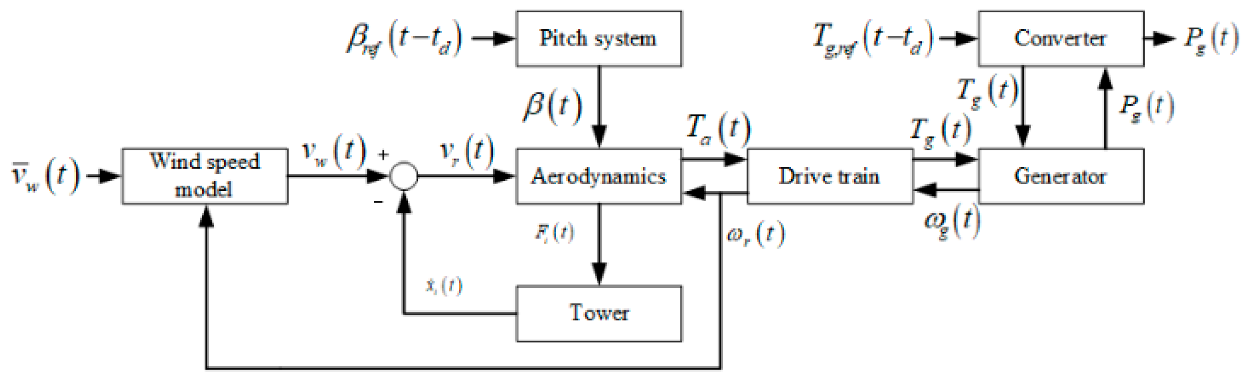
2. Model of a WECS with Delayed Inputs and an Unknown Part

To achieve the design objectives of this study, it is crucial to establish a high-precision mathematical model of the WECS. This model serves as the foundation for observer design and fault mathematical models, and it also provides the original data for the application of PDF fitting. The WECS model presented in this paper is derived from the Danish standard three-pitch horizontal-axis active-yaw WECS developed by KK Wind Solutions in Ikast, Denmark. The system comprises several subsystems: the wind model, pitch system, aerodynamics, wind turbine tower, drive train, generator, and converter. Figure 1 illustrates the relationships among the subsystems, considering the interaction effects.

The delays in this system occur in the pitch angle actuators and the converter, influenced by communication distance, signal interference, communication mode, and communication equipment. For a single WECS, the various delays can be consolidated into a uniform-sized delay factor for further study. Consequently, this paper defines a uniform symbol $t_d$ for the system delays, taking the maximum value of the delays. The mathematical model of the WECS adopted in this paper is based on prior work [37], which neglects the dynamic aerodynamic forces $F_t\left(t\right)$ acting on the wind turbine tower and the resulting tower displacement $x_t\left(t\right)$, as well as the motion control model of the active yaw system. The mathematical model for each part is as follows.

2.1. The Pitch System Model

The pitch system is represented as a second-order system with a communication delay, described as follows:

$${\ddot{\beta }}_i\left(t\right)=-2\zeta {\omega }_n{\dot{\beta }}_i\left(t\right)-{\omega }_n^2{\dot{\beta }}_i\left(t\right)+{\omega }_n^2{\beta }_{ref,i}\left(t-t_d\right)$$

(1)

for $i=1,2,3$, where ${\beta }_i\left(t\right)$ represents the pitch angle [°], ${\beta }_{ref,i}\left(t-t_d\right)$ represents the delayed reference input of ${\beta }_i\left(t\right)$ [°], ${\omega }_n$ represents the natural frequency of the pitch actuators, $\zeta$ represents the damping ratio of the pitch actuators, and $i$ represents the $i\text{-}th$ pitch actuator. This provides a generic description of a single pitch for a general three-pitch WECS. The simulation data indicate slight differences among the three pitch angles due to the differing phases among the pitches. In this paper, it is assumed that the three pitches have the same angle, as described by the above formula.

2.2. The Aerodynamics Model

The aerodynamics can be modeled as an unknown nonlinear system with two variables, described as follows:

$$T_a\left(t\right)=\rho \pi R^2{v}_r^3\left(t\right)C_p\left(\lambda \left(t\right),\beta \left(t\right)\right)/2{\omega }_r\left(t\right)$$

(2)

where $T_a\left(t\right)$ represents the aerodynamic torque applied to the rotor [Nm], ${\omega }_r\left(t\right)$ represents the rotor angular velocity [rad/s], $v_r\left(t\right)$ represents the effective wind speed on the rotor [m/s], and $C_p\left(\lambda \left(t\right),\beta \left(t\right)\right)$ stands for the power coefficient, which is a data set related to the tip-speed ratio $\lambda \left(t\right)$ and the effective pitch angle $\beta \left(t\right)$. Although there is no explicit formula for it, it can be obtained by consulting lookup tables. Such an unknown nonlinear aerodynamic mathematical model exhibits superior accuracy and dynamic response compared to conventional linear approximation models. The actual wind $v_w\left(t\right)$ acting on the pitches causes displacements of the turbine tower, from which the rotor’s effective wind speed $v_r\left(t\right)$ is obtained. As previously assumed, the turbine tower remains stationary. Consequently, the effective wind speed $v_r\left(t\right)$, which has been calculated, is applied in this study.

2.3. The Drivetrain Model

The drivetrain consists of a low-speed shaft connected to the pitch, a high-speed shaft connected to the generator rotor, and a gearbox that connects the low-speed shaft and the high-speed shaft. The aerodynamic torque exerts a driving force on the pitch, causing the low-speed shaft to rotate. This rotation is transmitted through the gearbox to drive the generator. The drive train is modeled by three first-order differential equations, described as:

$${\dot{\omega }}_r\left(t\right)={\displaystyle \frac{T_a\left(t\right)}{J_r}}-{\displaystyle \frac{K_{dt}{\theta }_{\Delta }\left(t\right)}{J_r}}-{\displaystyle \frac{\left(B_{dt}+B_r\right)}{J_r}}{\omega }_r\left(t\right)+{\displaystyle \frac{B_{dt}}{N_g{J}_r}}{\omega }_g\left(t\right)$$

(3)

$${\dot{\omega }}_g\left(t\right)={\displaystyle \frac{K_{dt}}{N_g{J}_g}}{\theta }_{\Delta }\left(t\right)+{\displaystyle \frac{B_{dt}}{N_g{J}_g}}{\omega }_r\left(t\right)-\left({\displaystyle \frac{B_{dt}}{N_g^2{J}_g}}+{\displaystyle \frac{B_g}{J_g}}\right){\omega }_g\left(t\right)-{\displaystyle \frac{T_g\left(t\right)}{J_g}}$$

(4)

$${\dot{\theta }}_{\Delta }\left(t\right)={\omega }_r\left(t\right)-{\displaystyle \frac{1}{N_g}}{\omega }_g\left(t\right)$$

(5)

where ${\theta }_{\Delta }\left(t\right)$ represents the torsion angle of the drive train [rad/s], ${\omega }_g\left(t\right)$ represents the angular velocity of the generator rotor [rad/s], and $T_g\left(t\right)$ represents the generator rotor torque [Nm].

2.4. The Converter Model

The converter is modeled as a first-order system with a time delay, described as:

$${\dot{T}}_g\left(t\right)=-{\displaystyle \frac{1}{{\tau }_g}}{T}_g\left(t\right)+{\displaystyle \frac{1}{{\tau }_g}}{T}_{g,ref}\left(t-t_d\right)$$

(6)

where ${\tau }_g$ represents the time constant and $T_{g,ref}\left(t-t_d\right)$ represents the delayed reference value of generator torque [Nm].

Consequently, the state-space model of a WECS with a delayed input and an unknown nonlinear component is constructed from the aforementioned subsystems. The model descriptions are presented as follows:

$$\begin{array}{l}\dot{X}\left(t\right)=AX\left(t\right)+B_2{U}_2\left(t-t_{dl}\right)+B_3\Phi +ED\left(t\right)\\ Y\left(t\right)=CX\left(t\right)+N\left(t\right)\end{array}$$

(7)

where $X\left(t\right)={\left[\begin{array}{cccccc}{\omega }_r\left(t\right)& {\omega }_g\left(t\right)& {\theta }_{\Delta }\left(t\right)& T_g\left(t\right)& {\beta }_i\left(t\right)& {\dot{\beta }}_i\left(t\right)\end{array}\right]}^T$, $U_2\left(t-t_{dl}\right)={\left[\begin{array}{cc}{T}_{g,ref}\left(t-t_{g,d}\right)& {\beta }_{ref,i}\left(t-t_d\right)\end{array}\right]}^T$, $\Phi =\left[{\displaystyle \frac{v_r^3\left(t\right)}{{\omega }_r\left(t\right)}}{C}_p{\left(\lambda \left(t\right),\beta \left(t\right)\right)}_m\right]$, $A=\left[\begin{array}{cccccc}{A}_{11}& A_{12}& A_{13}& 0& 0_{1\times 3}& 0_{1\times 3}\\ A_{21}& A_{22}& A_{23}& A_{24}& 0_{1\times 3}& 0_{1\times 3}\\ 1& A_{32}& 0& 0& 0_{1\times 3}& 0_{1\times 3}\\ 0& 0& 0& A_{44}& 0_{1\times 3}& 0_{1\times 3}\\ 0_{3\times 1}& 0_{3\times 1}& 0_{3\times 1}& 0_{3\times 1}& 0_{3\times 3}& I_{3\times 3}\\ 0_{3\times 1}& 0_{3\times 1}& 0_{3\times 1}& 0_{3\times 1}& A_{65}& A_{66}\end{array}\right]$, $B_2=\left[\begin{array}{cc}0& 0_{1\times 3}\\ 0& 0_{1\times 3}\\ 0& 0_{1\times 3}\\ B_{241}& 0_{1\times 3}\\ 0_{3\times 1}& 0_{3\times 3}\\ 0_{3\times 1}& B_{262}\end{array}\right]$, $B_3=\left[\begin{array}{c}{B}_{312}\\ 0\\ 0\\ 0\\ 0_{3\times 1}\\ 0_{3\times 1}\end{array}\right]$, $C=\left[\begin{array}{cccccc}0& 1& 0& 0& 0_{1\times 3}& 0_{1\times 3}\\ 0& 0& 0& 1& 0_{1\times 3}& 0_{1\times 3}\end{array}\right]$, $A_{11}=-{\displaystyle \frac{\left(B_{dt}+B_r\right)}{J_r}}$, $A_{12}={\displaystyle \frac{B_{dt}}{N_g{J}_r}}$, $A_{13}=-{\displaystyle \frac{K_{dt}}{J_r}}$, $A_{21}={\displaystyle \frac{B_{dt}}{N_g{J}_g}}$, $A_{22}=-\left({\displaystyle \frac{B_{dt}}{N_g^2{J}_g}}+{\displaystyle \frac{B_g}{J_g}}\right)$, $A_{23}={\displaystyle \frac{K_{dt}}{N_g{J}_g}}$, $A_{24}=-{\displaystyle \frac{1}{J_g}}$, $A_{32}=-{\displaystyle \frac{1}{N_g}}$, $A_{44}=-{\displaystyle \frac{1}{{\tau }_g}}$, $A_{65}=-{\omega }_n^2{I}_{3\times 3}$, $A_{66}=-2\zeta {\omega }_n{I}_{3\times 3}$, $B_{241}={\displaystyle \frac{1}{{\tau }_g}}$, $B_{262}={\omega }_n^2{I}_{3\times 3}$, $B_{312}={\displaystyle \frac{\rho A}{2J_r}}$. $ED\left(t\right)$ represents a white noise that affects all states. Given that noise signals are incorporated into the mathematical model, this paper assumes that the state vector $X\left(t\right)$ represents the measured value vector.

3. Observer Design, Faults Setting, and SONN Construction

This section is comprised of four parts: the improved set-value observer design, the pitch angle actuator faults modeling approach, the design for the SOCNN, and the design for the SOMNN. The details are provided below.

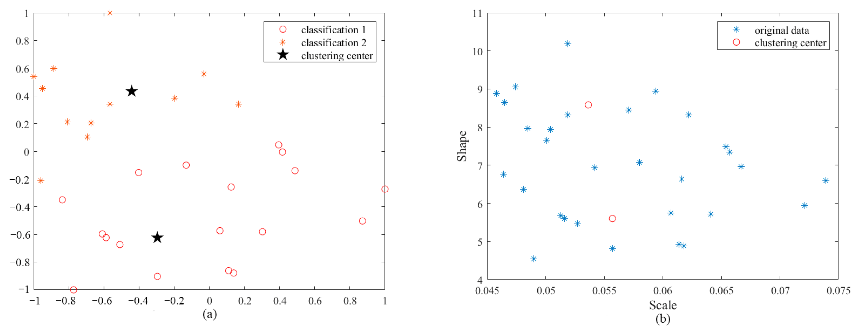
3.1. Design of Improved SVO

The general state-space function of a continuous system with delayed inputs and unknown nonlinear parts is as follows:

$$\begin{array}{l}\dot{x}\left(t\right)=ax\left(t\right)+b_1{u}_1\left(t\right)+b_2{u}_2\left(t_{id}\right)+b_3\varphi \left(x_{un}\left(t\right),u_3\left(t\right)\right)+ed\left(t\right)\\ y\left(t\right)=cx\left(t\right)+n\left(t\right)\end{array}$$

(8)

where $b_3\varphi \left(x_{un}\left(t\right),u_3\left(t\right)\right)$ represents the unknown nonlinear item, $\varphi \left(x_{un}\left(t\right),u_3\left(t\right)\right)$ represents the result vector of each sample of the unknown nonlinear item, $x_{un}\left(t\right)$ represents the variable related to the state $x\left(t\right)$ in the unknown nonlinear part, and $u_3\left(t\right)$ represents the variable independent of $x\left(t\right)$. For the above system, an improved SVO is designed to estimate the states within an adjustable interval. The form of the improved SVO is presented as follows:

$$\dot{\widehat{x}}\left(t\right)=\left(a-l_{un}c\right)\widehat{x}\left(t\right)+b_1{u}_1\left(t\right)+b_2{u}_2\left(t_{id}\right)+b_3\varphi \left({\widehat{x}}_{un}\left(t\right),u_3\left(t\right)\right)+l_{un}y\left(t\right)$$

(9)

Thus, the estimation error $e\left(t\right)=\widehat{x}\left(t\right)-x\left(t\right)$ is expressed as follows:

$$\dot{e}\left(t\right)=\left(a-l_{un}c\right)e\left(t\right)+l_{un}n\left(t\right)-ed\left(t\right)+b_3\left(\varphi \left({\widehat{x}}_{un}\left(t\right),u_3\left(t\right)\right)-\varphi \left(x_{un}\left(t\right),u_3\left(t\right)\right)\right)$$

(10)

By applying the Euler approximation algorithm, function (10) can be approximated and discretized. The approximated discretization result can be divided into a linear part and a nonlinear part. By applying the strong positive D-invariance and the global Lipschitz condition to the linear part, the inequalities concerning its upper and lower bounds can be obtained. The inequalities about the upper and lower bounds of the nonlinear bounded part are easily known. The approximated discretization results can be seen to be convergent by combining two inequalities through the strong positive D-invariance, ensuring the discrete estimation error is convergent. Therefore, the continuous estimation error is also convergent. By substituting several different sets of state vertices and changing the corresponding parameters into the inequality considering the worst case, the range of values for each element of the gain matrix $l_{un}$ can be obtained by solving the inequality. Taking the value of the gain matrix $l_{un}$ several times and substituting it into function (10) for the simulation experiments allows for the determination of the specific value of the gain matrix $l_{un}$. It is important to note that the specific value of $l_{un}$ is not unique, and the different values may affect the subsequent experimental procedures and the results. The experimental procedure, the detailed observer design process, the convergence proof process, and the gain matrix $l_{un}$ calculation process have been described in detail in [4], as well as the performance of the state estimate and the differences with traditional observers. These processes will not be repeated in this paper.

3.2. Modelling of Pitch Angle Actuators Faults

This paper focuses on the fault diagnosis of actuator faults in the pitch system 2.1. The most common faults of pitch angle actuators include hydraulic pump wear, hydraulic leakage, and high air content in the hydraulic oil [37]. The mathematical models of these faults can be described as variable-parameter models of the pitch system Section 2.1. Consequently, a simplified fault model is proposed as follows:

$$\begin{array}{l}{\ddot{\beta }}_i\left(t\right)=-2\tilde{\zeta }\left(t\right){\tilde{\omega }}_n\left(t\right){\dot{\beta }}_i\left(t\right)-{\tilde{\omega }}_n^2\left(t\right){\beta }_i\left(t\right)+{\tilde{\omega }}_n^2{\beta }_{ref}\left(t-t_d\right)\\ \tilde{\zeta }\left(t\right)=\left(1-{\alpha }_m\left(t\right)\right)\zeta +{\alpha }_m\left(t\right){\zeta }_i\\ {\tilde{\omega }}_n\left(t\right)=\left(1-{\alpha }_m\left(t\right)\right){\omega }_n+{\alpha }_m\left(t\right){\omega }_{n,i}\end{array}$$

(11)

where ${\alpha }_m\left(t\right)$ represents the fault conditions, $m=pw,hl,ha$. For hydraulic pump wear, ${\alpha }_{pw}\left(t\right)\in \left[0,1\right]$ represents the indicator of hydraulic pump wear, and its change rate is ${\dot{\alpha }}_{pw}\left(t\right)\ge 0$. This fault is irreversible before fault treatment. The pump pressure drops to 75% of the normal pressure when ${\alpha }_{pw}=1$. For hydraulic leakage, ${\alpha }_{hl}\left(t\right)\in \left[0,1\right]$ represents the indicator of hydraulic leakage. Similar to ${\alpha }_{pw}\left(t\right)$, the change rate of ${\alpha }_{hl}\left(t\right)$ satisfies ${\dot{\alpha }}_{hl}\left(t\right)\ge 0$. The pump pressure drops to 50% of the normal pressure when ${\alpha }_{hl}=1$. For high air content in hydraulic oil, ${\alpha }_{ha}\left(t\right)\in \left[0,1\right]$ represents the indicator of air content in hydraulic oil. Unlike ${\alpha }_{pw}\left(t\right)$ and ${\alpha }_{hl}\left(t\right)$, the change rate of ${\alpha }_{ha}\left(t\right)$ can be either positive or negative. When ${\alpha }_{ha}=1$, the air content in hydraulic oil is 15%, which is considered to be an extreme case.

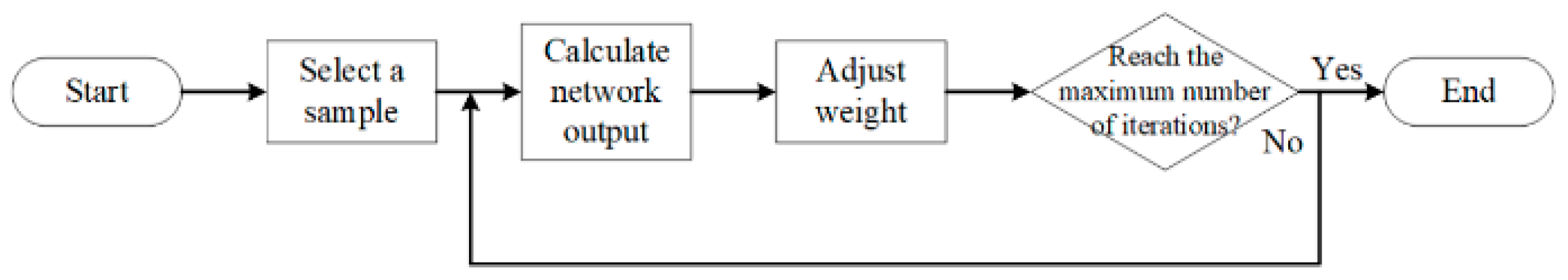
3.3. Design of SOCNN

An SOCNN is an unsupervised neural network with a two-layer structure, as illustrated in Figure 2.

At the beginning of the computation, the weights of the input layer are randomly assigned to the competitive layer, and each neuron has an equal probability of winning. After a single computation, a single output neuron is designated as the winner and labeled one. This neuron’s excitability is further enhanced by the weight adjustment, while the non-winning neurons are labeled zero and remain unchanged by the weight adjustment. The competitive neural network learns the distribution of the training samples through competitive learning. Each training sample is associated with an excited neuron in the competitive layer. When a new sample is input, it can be clustered according to the excited neurons. Figure 3 shows the flowchart of a single iteration of the SOCNN.

The learning steps for SOCNN are as follows:

• Initialize the runtime environment;
• Build the network. Assume that the sample data $p$ is divided into two categories, initializing weights $w$ to random values and tentatively set the learning rate $net.it=0.2$;
• Normalize the samples and feed them serially into the network;
• Identify the winning neuron. Calculate network output $yout=w*p$. Find the neuron $y_k$ with the maximum value in the output neuron $yout$ and designated it as the winning neuron;
• Adjust weights. For the winning neuron $y_k$, adjust the corresponding weights according to $\Delta w_{rk}=\eta \left(p_r-w_{ik}\right)$, while the weights of the remaining neurons are not adjusted;
• Determine whether there is convergence. Repeat steps 4 to 5. Set the maximum number of iterations. The program will automatically stop after reaching this certain number of iterations;
• Test and label. After the weights stop updating, feed the original training samples into the network for category labeling.

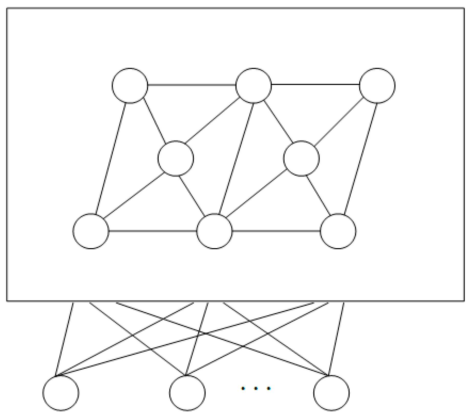
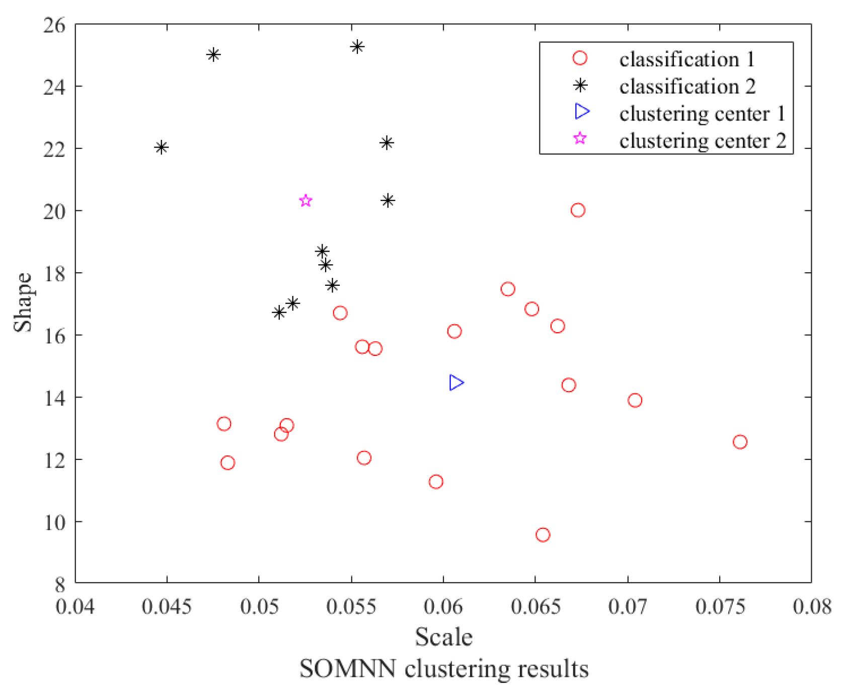
3.4. Design of SOMNN

SOMNNs are analogous to SOCNNs in that they are unsupervised learning networks with competitive neurons. The distinguishing feature of SOMNN is its ability to discern the topology of the input vectors in addition to learning the distribution of input samples. This requires the involvement of multiple neurons to achieve pattern classification. The structure of a SOMNN is depicted in Figure 4.

The learning steps for SOMNN are as follows:

• Initialize the runtime environment;
• Input training samples and normalize them;
• Build the network. Determine the dimension of the weight matrix based on the dimensions of the input and output vectors. Set the learning rate of change formula as follows:

  $$l{r}_m=l{r}_{\max }-{\displaystyle \frac{m}{N}}\left(l{r}_{\max }-l{r}_{\min }\right)$$

  (12)

  where $m$ represents the current iteration number, $N$ represents the total number of iterations, $l{r}_{\max }$ represents the maximum value of the learning rate, and $l{r}_{\min }$ represents the minimum value of the learning rate. The radius of the neighborhood of the optimal node is calculated as follows:

  $$d=d_{\max }-{\displaystyle \frac{m}{N}}\left(d_{\max }-d_{\min }\right)$$

  (13)

  where $d_{\max }$ represents the maximum value of the radius of the neighborhood, and $d_{\min }$ represents the minimum value of the radius of the neighborhood;
• Iterative updating. Randomly draw a vector from the sample set and feed it into the network. Calculate the Euclidean distance between the weights and the input vector using the following function:

  $$d_k=\sqrt{{\displaystyle \sum _{m=1}^n{\left(x_m-w_{mk}\right)}^2}}$$

  (14)

  Find the minimum value of $d_k$ and mark as $d_K$; the neuron corresponding to $d_K$ is the winning neuron. Then, the learning rate for the current number of iterations and the neighborhood size parameter are calculated to determine the neighborhood domain. The weights are updated for the neurons within the neighborhood;
• Determine whether the maximum number of iterations has been reached. If not, return to step 4 until the end of training;
• Obtain the trained network, feed the training samples into the network, and obtain the clustering results.

4. Design of Fault Diagnosis Strategies

This section presents fault diagnosis strategies based on improved SVO, PDF, and SONN for WECS pitch actuator faults, employing offline design and online testing methods. The fault diagnosis strategies can be categorized into two types based on the application of two different kinds of SONNs. The first type is the fault diagnosis strategy employing SOCNN, denoted as FDS-ISVO-PDF-SOCNN. The second type is the fault diagnosis strategy employing SOMNN, denoted as FDS-ISVO-PDF-SOMNN. Although the two fault diagnosis strategies exhibit slight differences, the offline design process and the basis for fault diagnosis remain consistent. The following Figure 5 outlines the flowchart of offline design.

To determine the most suitable distribution algorithm for fitting the probability density function of the data, we tested the fitting results of the Gaussian distribution, Gamma distribution, and Weibull distribution separately. We used the ${\chi }^2$ test and the log-likelihood value test to evaluate the fitting results of the three distributions. The visual graphs of the fitting results for the three distributions are shown in Figure 6, and their ${\chi }^2$ test and log-likelihood value test results are presented in

Table 1. PDF fitting accuracy test results for the three distribution algorithms. The tested data are the No. 3 preprocessed dataset from Fault Case 1.

Distribution Algorithm	${\mathit{\chi }}^2$ Test	Log-Likelihood Value Test
Gaussian distribution	$h=1,p=7.2488\times {10}^{-319}$	$-4.8624\times {10}^3$
Gamma distribution	$h=0,p=0.3608$	$5.4734\times {10}^4$
Weibull distribution	$h=1,p=4.7708\times {10}^{-66}$	$1.3147\times {10}^4$

.

As illustrated in Figure 6, the fitting performance of the PDF based on the Gamma distribution surpasses that of the Gaussian distribution and is comparable to that of the Weibull distribution. We employed the ${\chi }^2$ test and the log-likelihood value test to evaluate the three distribution algorithms. The ${\chi }^2$ test yields two values, $h$ and $p$. The $h$ indicates whether to reject the null hypothesis, where $h=1$ signifies the rejection of the null hypothesis, implying that the two samples originate from different distributions, and $h=0$ suggests that the null hypothesis cannot be rejected, indicating that the two samples may come from the same distribution. The $p$ is used to assess the similarity between the distributions of the two samples. A larger $p$ denotes a greater similarity between the sample distributions, while a smaller $p$ indicates less similarity. The log-likelihood value test provides only the log-likelihood value, where a higher log-likelihood value suggests that the tested data better conforms to the specific distribution under the current parameters. As can be inferred from Table 1, the fitting degree of the PDF based on the Gamma distribution is significantly better than that of the other two distribution algorithms. Consequently, the offline design of the fault diagnosis strategy adopts the Gamma distribution for PDF fitting.

Once the fault diagnosis strategy design is complete, the subsequent step is to perform an online fault diagnosis. The FDS in this paper involves inputting the obtained processed pitch angle estimation error data $d{e}_{\beta }\left(t\right)$ into the PDFs $F_{C{r}_j{e}_{\beta -tr-SOCNN,i}}$ and $F_{C{r}_j{e}_{\beta -tr-SOMNN,i}}$ to derive the scalar values $SV\beta \left(t\right)$. Thus, the faults can be diagnosed based on the following assumptions:

$$\begin{array}{l}SV\beta \left(t\right)=0\Rightarrow fault-free\\ SV\beta \left(t\right)>0\Rightarrow faulted\end{array}$$

(15)

Define the fault diagnosis time (FDT) $t_{od}=t_{fd}-t_{fo}$ to evaluate the quality of the FDS, where $t_{fo}$ represents the fault occurrence time and $t_{fd}$ represents the fault diagnosis time.

5. Simulation Studies and Discussion

This section includes four parts, including the parameters of WECS and the parameter setting of the ISVO, the fault diagnosis simulations of three fault cases, the fault diagnosis simulations, and the comparative studies of fault diagnosis performance.

5.1. Parameters Setting of the WECS and the ISVO

This paper chooses a 4.8 MW WECS benchmark model as the simulation object. The parameters are listed in

Table 2. Values of the WECS properties.

Symbol	Quantity	Value (Unit)
$B_r$	Viscous friction coefficient of the low-speed shaft	$7.11 \left(\mathrm{Nm}\left(\mathrm{rad}/\mathrm{s}\right)\right)$
$B_g$	Viscous friction coefficient of the high-speed shaft	$45.6 \left(\mathrm{Nm}\left(\mathrm{rad}/\mathrm{s}\right)\right)$
$J_r$	Moment of inertia of the low-speed shaft	$5.5\times {10}^7 {\mathrm{kgm}}^2$
$J_g$	Moment of inertia of the high-speed shaft	$390 {\mathrm{kgm}}^2$
$B_{dt}$	Torsional damping coefficient of the drive train	$775.49 \left(\mathrm{Nm}\left(\mathrm{rad}/\mathrm{s}\right)\right)$
$K_{dt}$	Torsional stiffness of the drive train	$2.7\times {10}^9 \left(\mathrm{Nm}/\mathrm{rad}\right)$
$N_g$	Ratio of the drive train	95
${\tau }_g$	Time constant of the first-order system	0.02
${\omega }_n$	Pitch actuator model natural frequency	$11.11 \left(\mathrm{rad}/\mathrm{s}\right)$
$\zeta$	Pitch actuator model damping ratio	0.6
$\rho$	Air density	$1.225 \left({\mathrm{kg}/\mathrm{m}}^3\right)$
$R$	Radius of the cross-section of the pitch sweep	$57.5 \left(\mathrm{m}\right)$

below.

Therefore, the coefficient matrices can be calculated. By choosing at least 10 different sets of vertexes $v_j$ and the corresponding matrices $f_i^{\mathrm{T}}$, $\eta =0.9$, and $\epsilon =1$, the range of each element of the matrix $l_{un}$ can be obtained as $l_{un}={\left[\begin{array}{cccccccccc}20& 14360& -0.6& 1& -0.6& -0.6& -0.6& -2.6& -2.6& -2.6\\ 243& 8400& 0.3& 0.4& 0.3& 0.3& 0.3& -110& -110& -110\end{array}\right]}^{\mathrm{T}}$.

The selection process of one vertex set $v_j$ is as follows. First, a random state is selected from one simulation result of the system (10). Second, an extreme value is randomly selected from the simulation curve of the selected state, and the corresponding simulation moment is recorded. The aforementioned state values are then combined into a vertex set $v_j$ for the purpose of calculating the gain matrix $l_{un}$. It is recommended that the aforementioned selection process be repeated at least 10 times in order to obtain a smaller range of $l_{un}$. The corresponding matrix $f_i^{\mathrm{T}}$ is generally selected as a unit matrix. In the rest of this section, the simulations of fault diagnosis results for three specific fault cases are presented. The simulation environment is MATLAB/SIMULINK 2022a. The simulation time is 100 s.

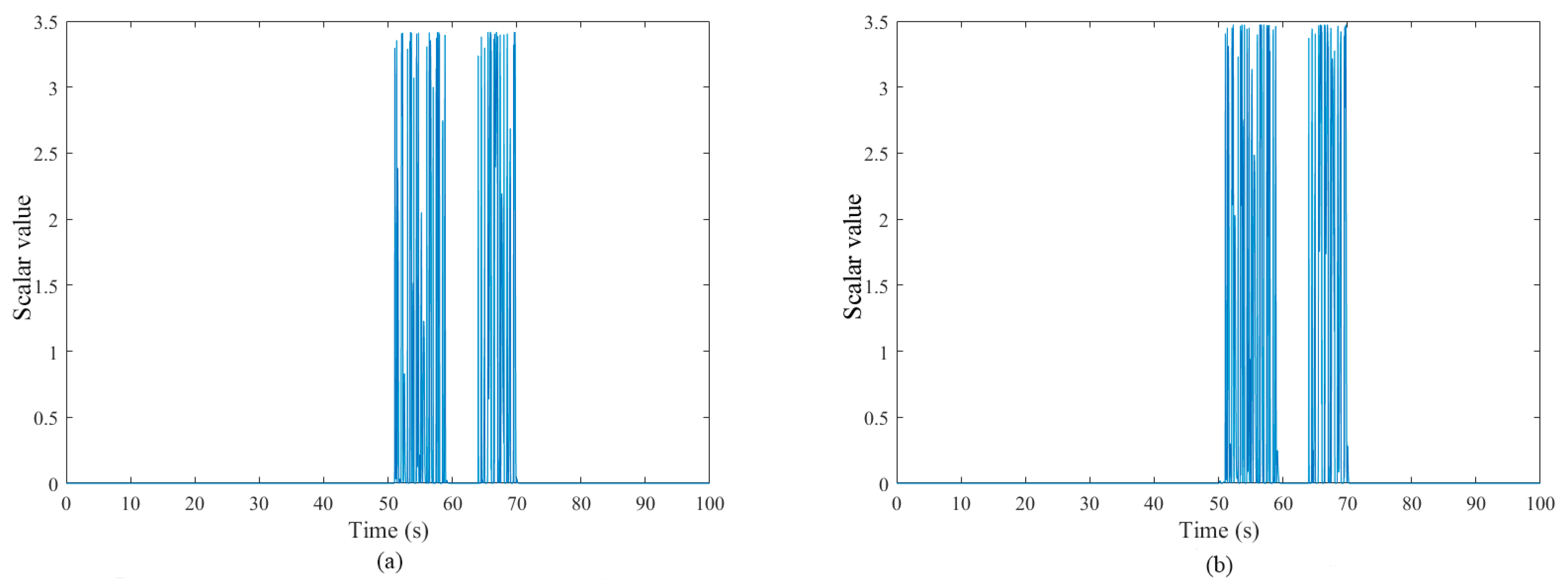
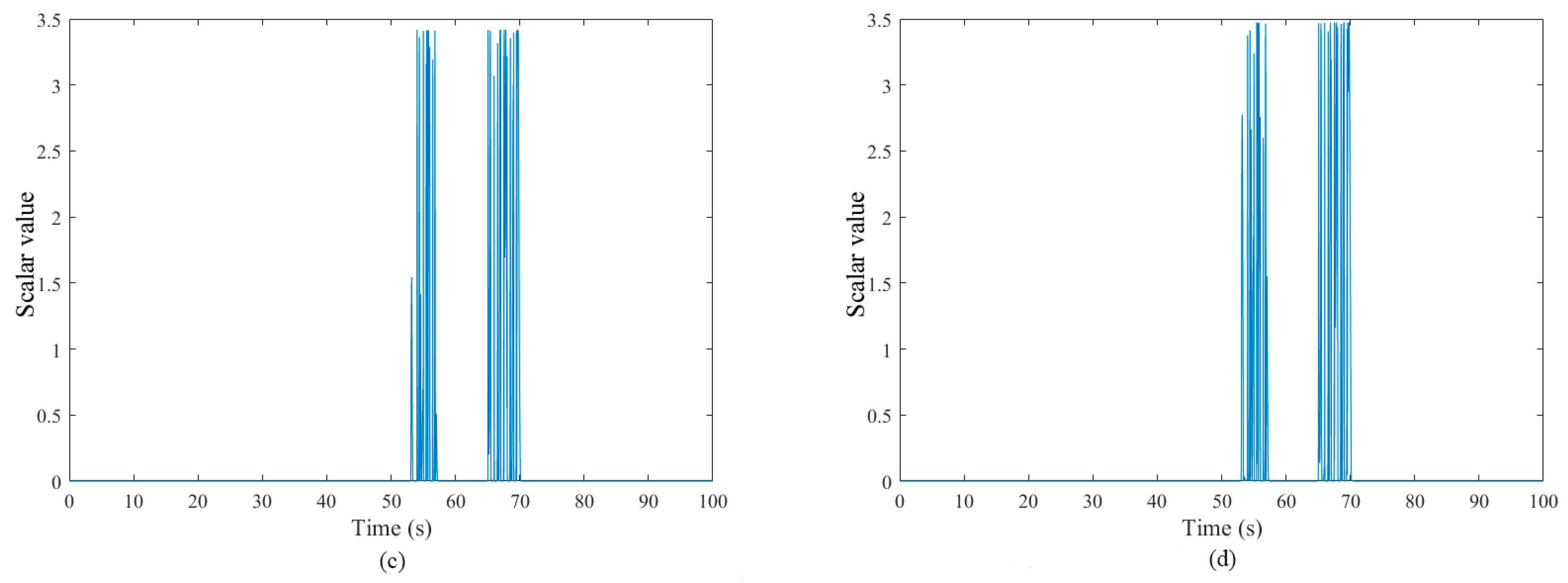
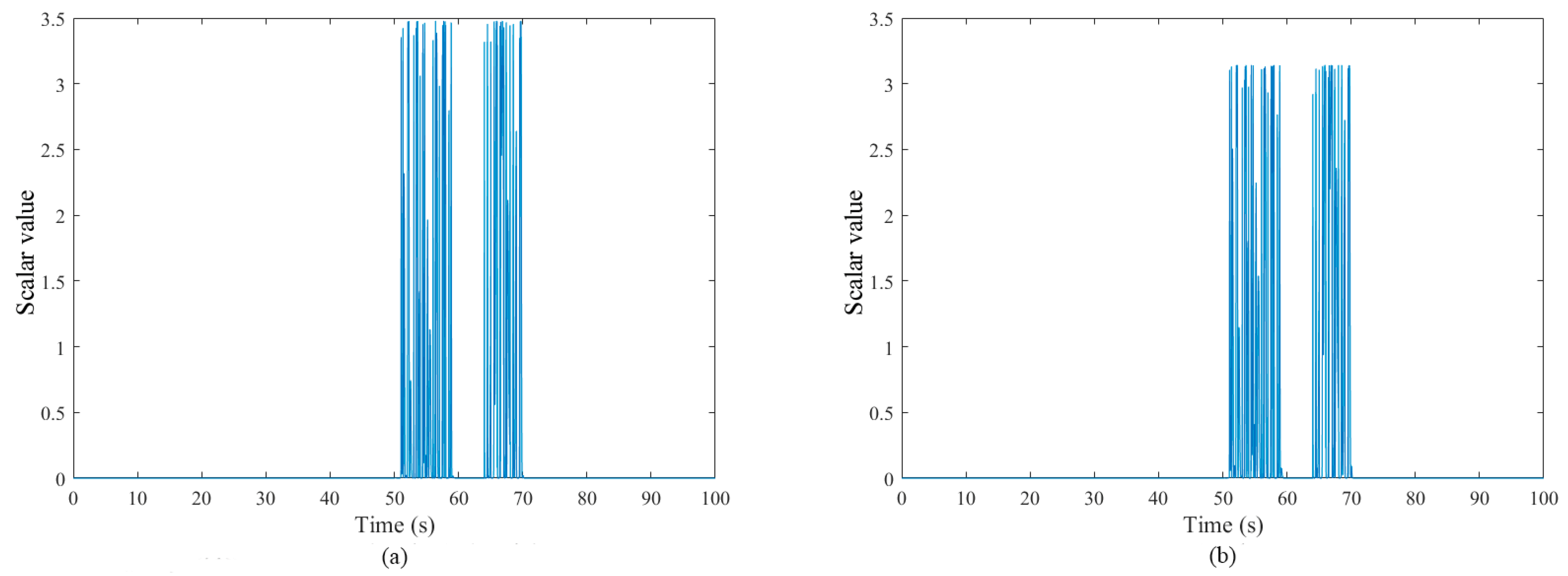
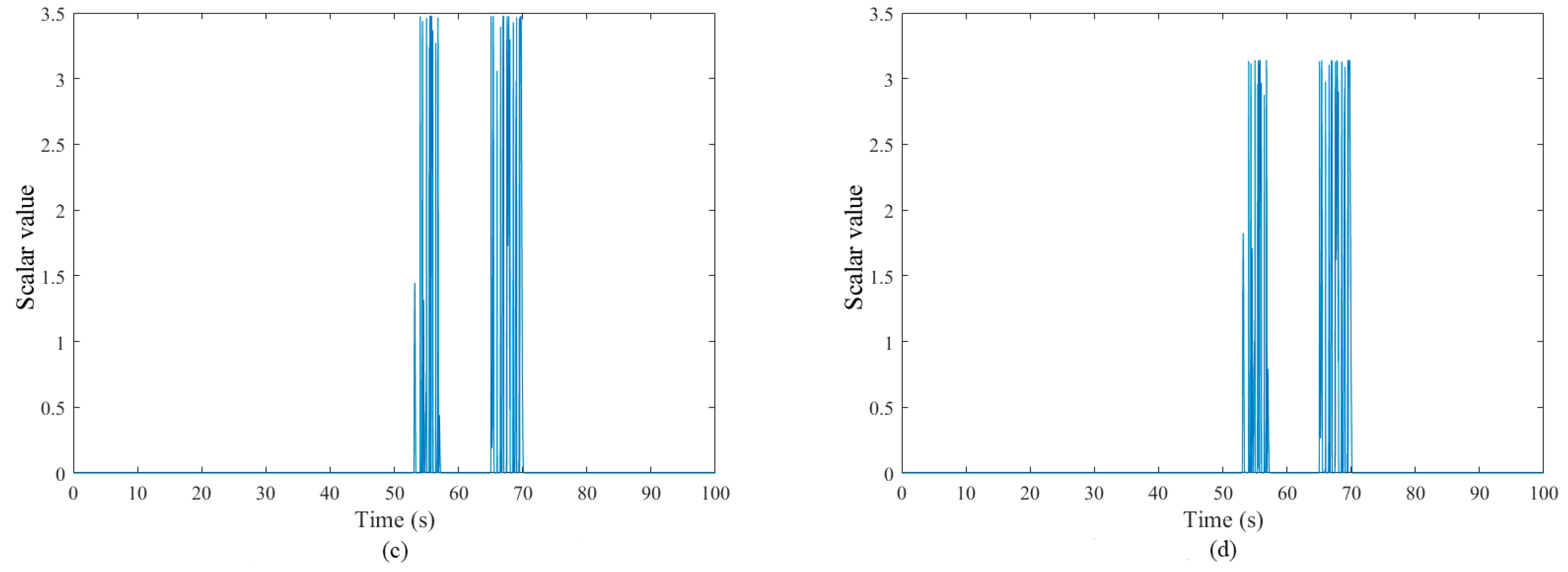
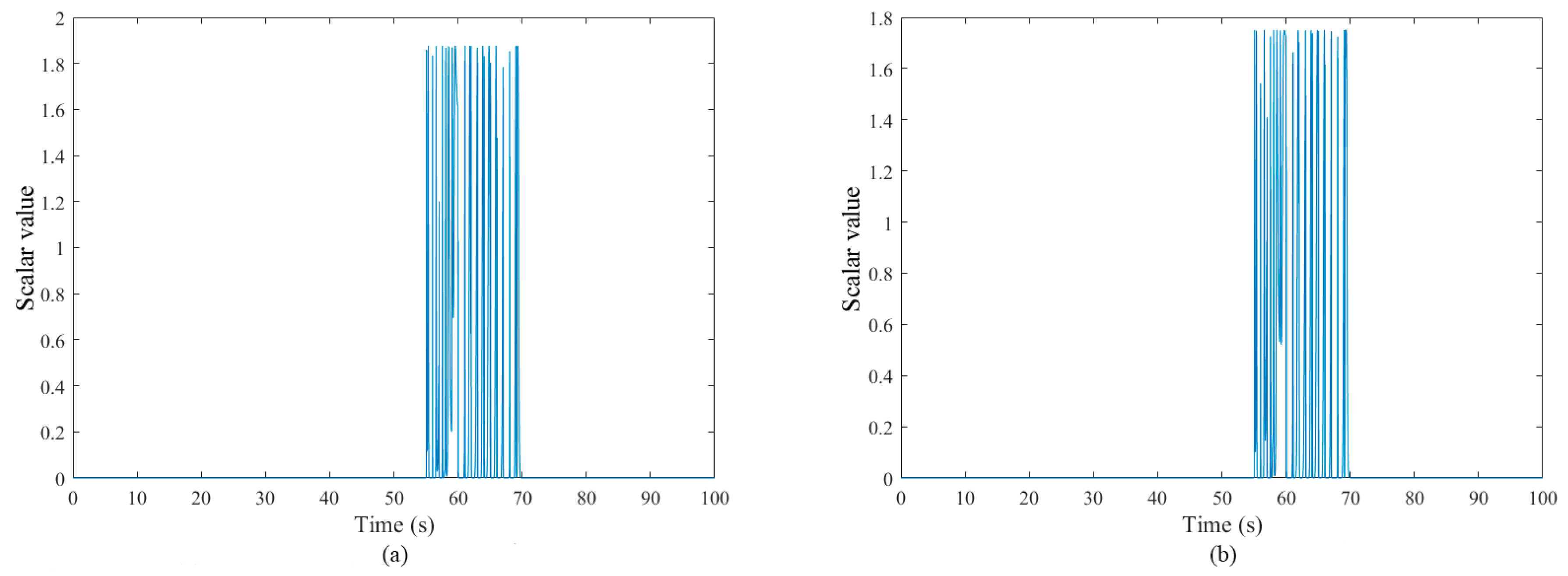
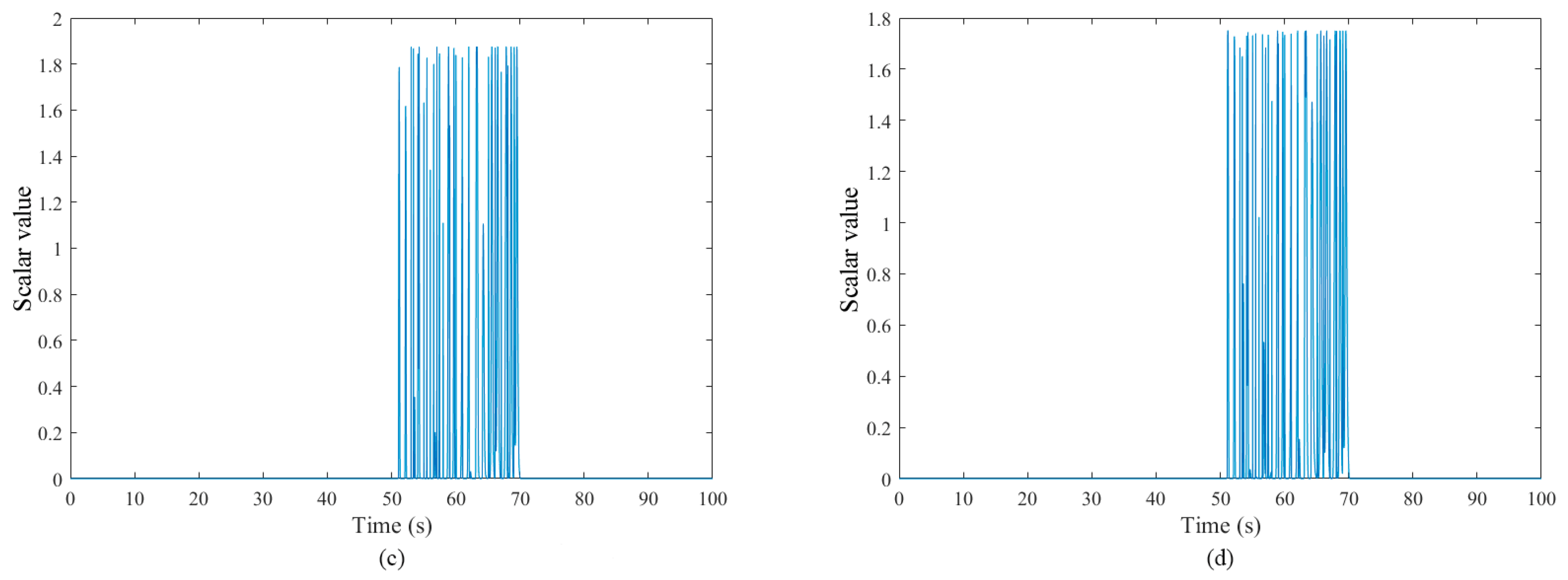
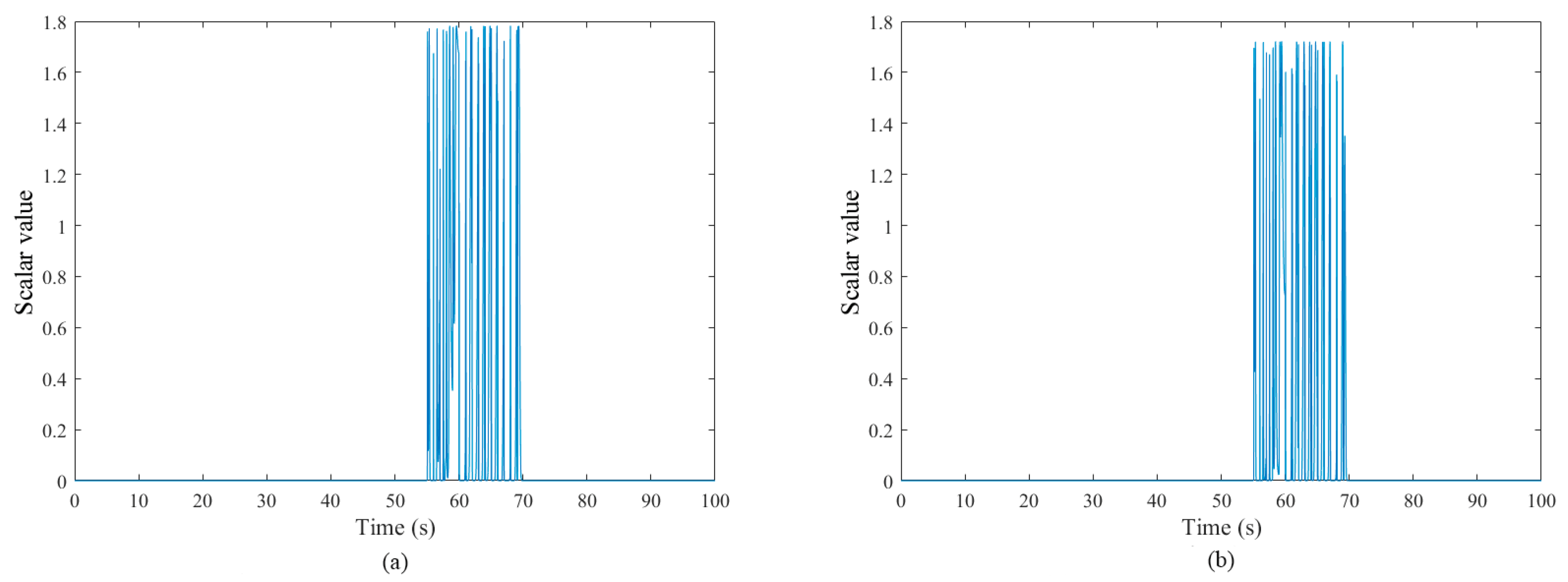
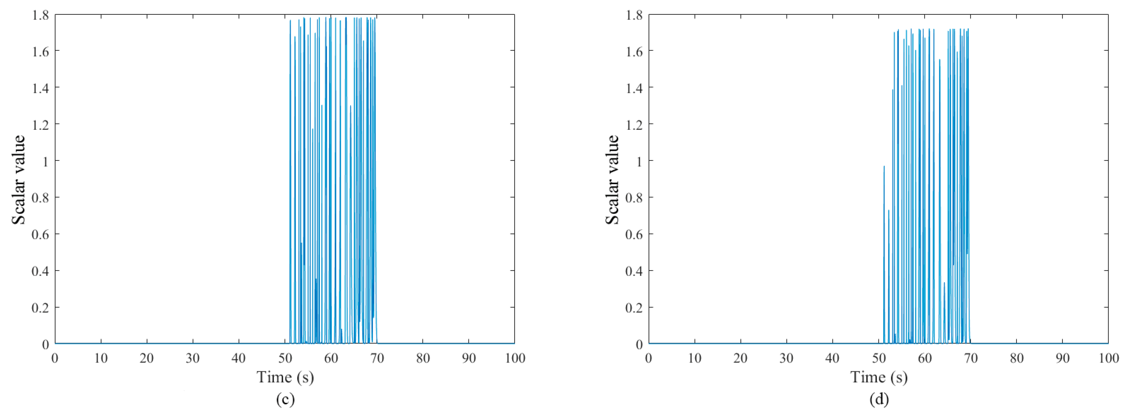
5.2. Fault Diagnosis Simulations and Analysis of Three Fault Cases

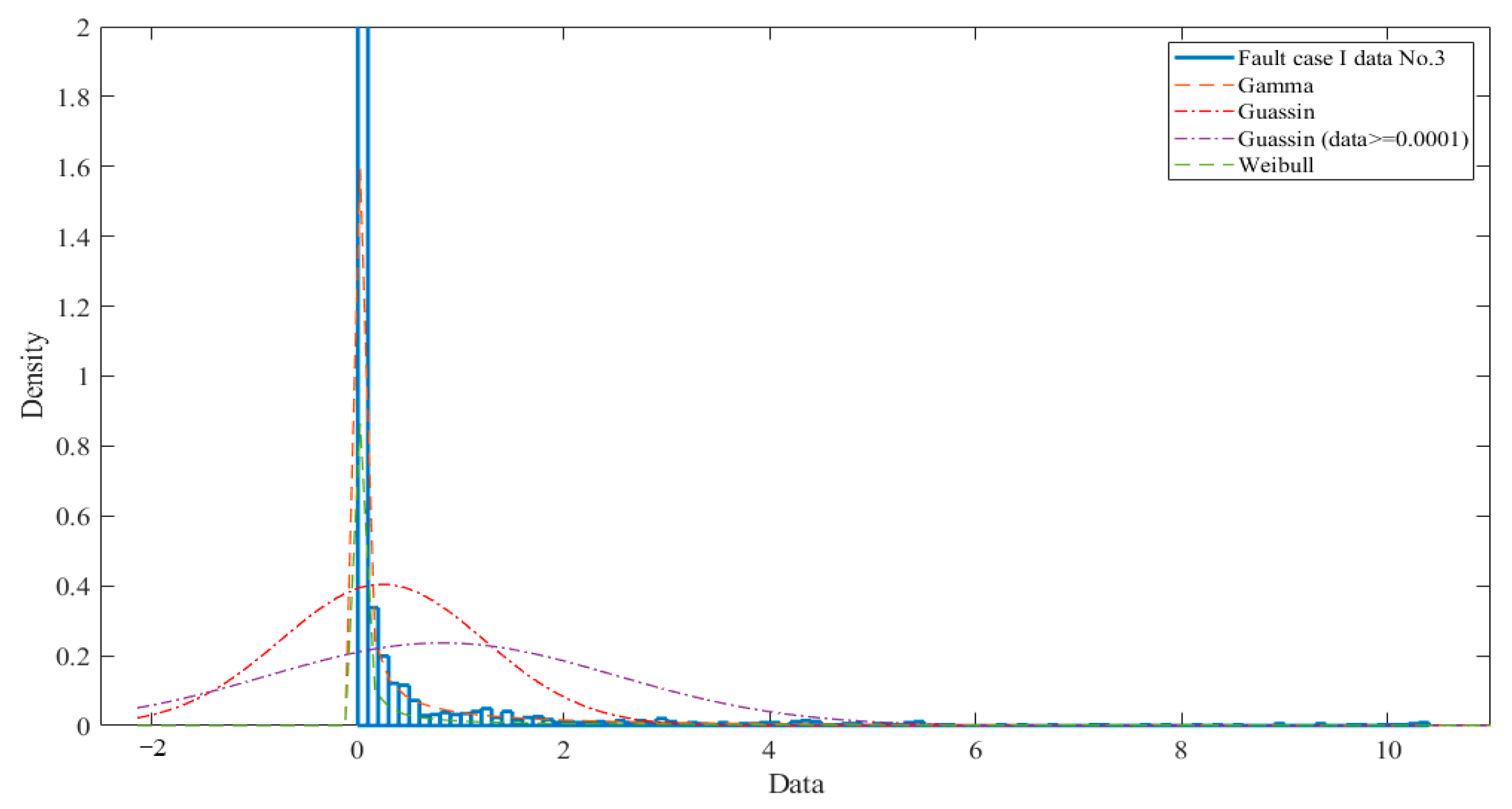
5.2.1. Fault Case I: Hydraulic Pump Wear

In actual engineering, hydraulic pump wear progresses relatively slowly, typically changing over the course of ten years. In this paper, it is assumed that hydraulic pump wear occurs at $t_{fo}=50.0 \mathrm{s}$. The indicator of hydraulic pump wear ${\alpha }_{pw}\left(t\right)$ increases linearly from zero to one in 10 s and remains constant for 10 s. Fault Case I ends at 70.0 s. By performing the offline design step of the fault diagnosis strategy, the SOCNN clustering results of the fitted PDF parameters can be obtained as shown below.

Figure 7 illustrates the results of applying the offline design steps of the fault diagnosis strategy for Fault Case I, where the SOCNN clustering results are two points $C{r}_1{e}_{\beta -tr-SOCNN,1}\left(0.0520, 5.8765\right)$ and $C{r}_2{e}_{\beta -tr-SOCNN,1}\left(0.0624, 4.2196\right)$ in Figure 7b. Subsequently, the PDFs of the Gamma distribution are constructed based on the two clustering results $C{r}_1{e}_{\beta -tr-SOCNN,1}$ and $C{r}_2{e}_{\beta -tr-SOCNN,1}$. Two sets of data are randomly selected from the training data $e_{\beta -tr,1}$ to test the two PDFs, labeled as $P_{case1-SOC-1}$ and $P_{case1-SOC-2}$. The test results are shown in Figure 8.

Figure 8 demonstrates that the two classes of PDFs constructed based on the SOCNN clustering results successfully pass the tests on the 15th and 23rd data randomly selected from the training data $e_{\beta -tr,1}$, indicating that the FDS-ISVO-PDF-SOCNN can effectively detect faults. The next section presents a similar simulation procedure and the results for SOMNN.

Figure 9 illustrates the results of applying the offline design steps of the fault diagnosis strategy for Fault Case I, where the SOMNN clustering results are represented by two points $C{r}_1{e}_{\beta -tr-SOMNN,1}\left(0.0496,6.1804\right)$ and $C{r}_2{e}_{\beta -tr-SOMNN,1}\left(0.0636,4.8090\right)$. Subsequently, the PDFs of the Gamma distribution are constructed based on the two clustering results $C{r}_1{e}_{\beta -tr-SOMNN,1}$ and $C{r}_2{e}_{\beta -tr-SOMNN,1}$, respectively. The 15th and 23rd training data $e_{\beta -tr,1}$ are applied to test the two PDFs, labeled as $P_{case1-SOM-1}$ and $P_{case1-SOM-2}$. The test results are shown in Figure 10.

Figure 10 demonstrates that the two classes of PDFs constructed based on the SOMNN clustering results can successfully pass the tests on the 15th and 23rd training data $e_{\beta -tr,1}$, indicating that the FDS-ISVO-PDF-SOMNN can effectively detect faults. The comparison of Figure 7 and Figure 9 reveals that the clustering results of SOCNN and SOMNN are disparate, despite using the same training data. The comparison of Figure 8 and Figure 10 shows that the test results differ for the same test data. The test results of the clustering center $C{r}_2{e}_{\beta -tr-SOMNN,1}$ of SOMNN are notably smaller than that of the corresponding clustering center $C{r}_2{e}_{\beta -tr-SOCNN,1}$ of SOCNN.

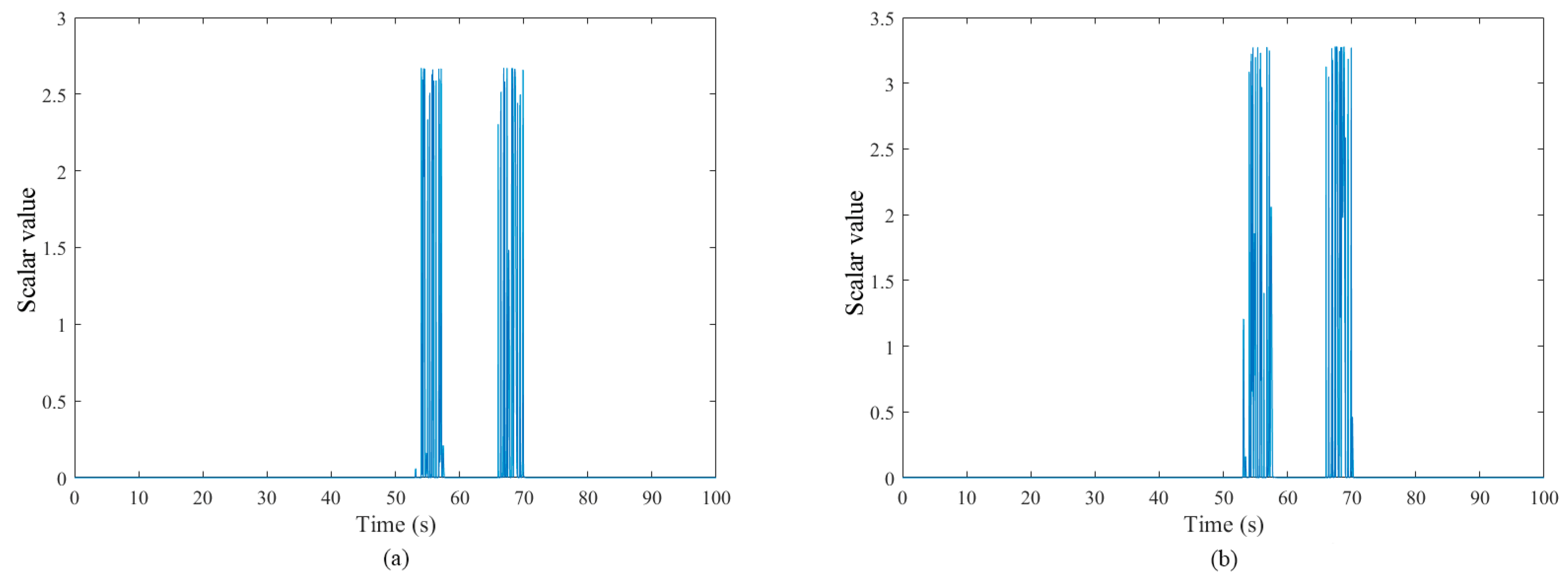
5.2.2. Fault Case II: Hydraulic Leak

In actual engineering, hydraulic leaks in the pitch system are typically short, usually within 2 min. In this paper, it is assumed that the hydraulic cylinder leaks at $t_{fo}=50.0 \mathrm{s}$. The indicator of hydraulic leak ${\alpha }_{hl}\left(t\right)$ increases linearly from zero to one in 10 s and remains constant for 10 s. The fault ends at 70.0 s. Similar to Fault Case I, by performing the offline design step of the fault diagnosis strategy, the SOCNN clustering results of the fitted PDF parameters can be obtained as shown below.

Figure 11 illustrates the results of applying the offline design steps of the fault diagnosis strategy for Fault Case II. With the SOCNN clustering results are two points $C{r}_1{e}_{\beta -tr-SOCNN,2}\left(0.0526,17.1720\right)$ and $C{r}_2{e}_{\beta -tr-SOCNN,2}\left(0.0659,12.7981\right)$, as shown in Figure 11b. Subsequently, PDFs of the Gamma distribution are constructed according to the two clustering results $C{r}_1{e}_{\beta -tr-SOCNN,2}$ and $C{r}_2{e}_{\beta -tr-SOCNN,2}$, respectively. Two sets of data are randomly selected from the training data $e_{\beta -tr,2}$ to test the two PDFs, labeled as $P_{case2-SOC-1}$ and $P_{case2-SOC-2}$. The test results are presented in Figure 12.

Figure 12 demonstrates that the two classes of PDFs constructed based on the SOCNN clustering results successfully pass the tests on the 6th and 25th data randomly selected from the training data $e_{\beta -tr,2}$, indicating that the FDS-ISVO-PDF-SOCNN is effective for fault diagnosis. Next, the similar simulation procedure and results for the SOMNN are discussed.

Figure 13 illustrates the results of applying the offline design steps of the fault diagnosis strategy for Fault Case II. With the SOMNN clustering results are two points $C{r}_1{e}_{\beta -tr-SOMNN,2}\left(0.0525,20.2972\right)$ and $C{r}_2{e}_{\beta -tr-SOMNN,2}\left(0.0606,14.4491\right)$. Subsequently, PDFs of the Gamma distribution are constructed according to the two clustering results $C{r}_1{e}_{\beta -tr-SOMNN,2}$ and $C{r}_2{e}_{\beta -tr-SOMNN,2}$, respectively. The 6th and 25th training data $e_{\beta -tr,2}$ are used to test the two PDFs, labeled as $P_{case2-SOM-1}$ and $P_{case2-SOM-2}$. The test results are presented in Figure 14.

Figure 14 demonstrates that the two classes of PDFs constructed based on the SOMNN clustering results can successfully pass the tests on the 6th and 25th training data $e_{\beta -tr,2}$, indicating that the FDS-ISVO-PDF-SOMNN effectively performs fault diagnosis. Comparing Figure 11 and Figure 13 reveals that the clustering results of SOCNN and SOMNN are distinct despite the use of the same training data. Additionally, comparing Figure 12 and Figure 14 indicates that the difference between test results is minimal. The test results of the clustering center $C{r}_1{e}_{\beta -tr-SOMNN,2}$ of SOMNN are slightly lower than that of the corresponding clustering center $C{r}_1{e}_{\beta -tr-SOCNN,2}$ of SOCNN.

5.2.3. Fault Case III: Hydraulic Oil Has a High Air Content

Similar to Fault Case II, the increased air content in the hydraulic oil results in a shorter duration of the fault. In this paper, it is assumed that the hydraulic cylinder of the hydraulics leaks at $t_{fo}=50.0 \mathrm{s}$. The indicator of hydraulic leak ${\alpha }_{ha}\left(t\right)$ increases linearly from zero to one in 10 s and remains constant for 10 s. The fault ends at 70.0 s. Following the same procedure as in Fault Case II, the SOCNN clustering results for the fitted PDF parameters are obtained and illustrated below.

Figure 15 illustrates the results of applying the offline design steps of the fault diagnosis strategy for Fault Case III. With the SOCNN clustering results are two points $C{r}_1{e}_{\beta -tr-SOCNN,3}\left(0.0536,8.5827\right)$ and $C{r}_2{e}_{\beta -tr-SOCNN,3}\left(0.0557,5.6021\right)$ in Figure 15b. Subsequently, the PDFs of the Gamma distribution are constructed according to the two clustering results $C{r}_1{e}_{\beta -tr-SOCNN,3}$ and $C{r}_2{e}_{\beta -tr-SOCNN,3}$, and two sets of data are randomly selected from the training data $e_{\beta -tr,3}$ to test the two PDFs, labeled as $P_{case3-SOC-1}$ and $P_{case3-SOC-2}$. The test results are presented in Figure 16.

Figure 16 demonstrates that the two classes of PDFs constructed from the SOCNN clustering results can successfully pass the tests on the 12th and 27th data randomly selected from the training data $e_{\beta -tr,3}$, indicating that the FDS-ISVO-PDF-SOCNN is effective for fault diagnosis. Next, the simulation procedure and results for SOMNN will be presented.

Figure 17 illustrates the results of applying the offline design steps of the fault diagnosis strategy for Fault Case III, where the clustering results of the SOMNN are represented by two points $C{r}_1{e}_{\beta -tr-SOMNN,3}\left(0.0507,7.4920\right)$ and $C{r}_2{e}_{\beta -tr-SOMNN,3}\left(0.0638,6.3437\right)$. Subsequently, PDFs of the Gamma distribution are constructed according to the two clustering results $C{r}_1{e}_{\beta -tr-SOMNN,3}$ and $C{r}_2{e}_{\beta -tr-SOMNN,3}$, respectively. The 12th and 27th training data $e_{\beta -tr,3}$ are used to test the two PDFs, labeled as $P_{case3-SOM-1}$ and $P_{case3-SOM-2}$. The test results are shown in Figure 18.

Figure 18 shows that the two classes of PDFs constructed based on the SOMNN clustering results can successfully pass the tests on the 12th and 27th training data $e_{\beta -tr,3}$, indicating that the FDS-ISVO-PDF-SOMNN is effective for fault diagnosis. The comparison of Figure 15 and Figure 17 reveals that the clustering results of the SOCNN and the SOMNN differ significantly, despite using the same training data. The comparison of Figure 16 and Figure 18 indicates that the difference between test results is minimal, with the primary discrepancy observed in the values obtained.

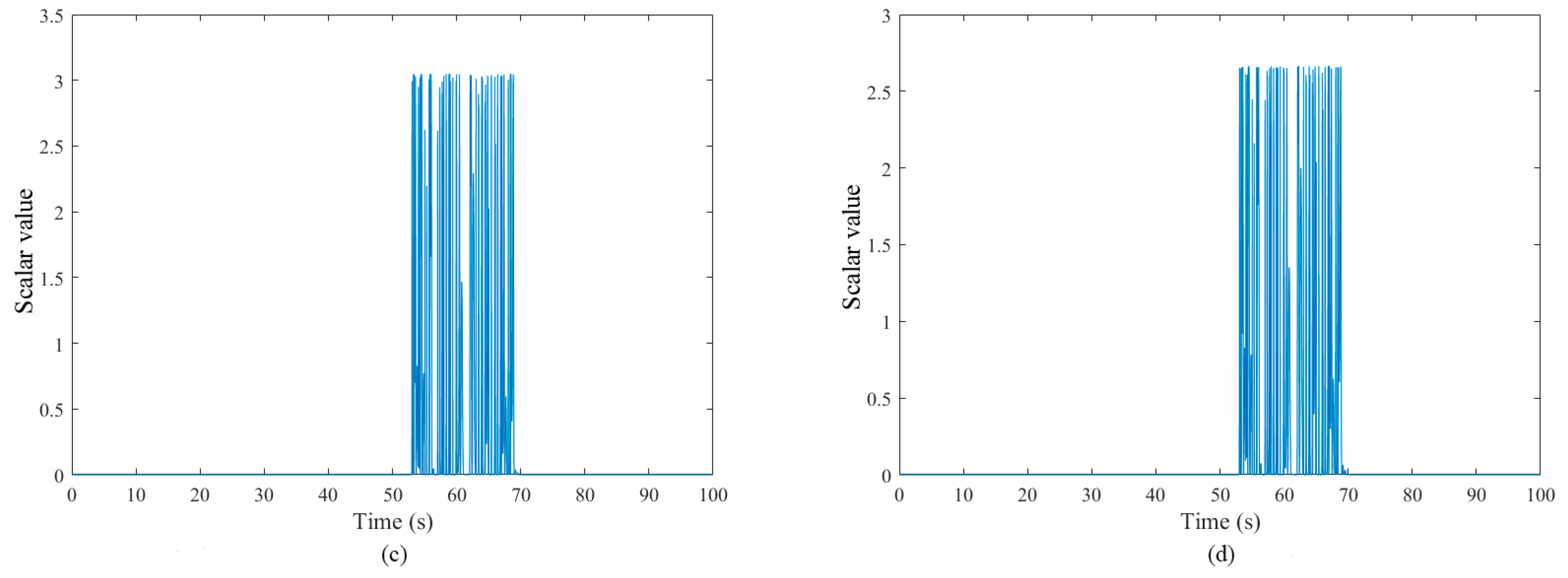
5.3. Comparative Studies for Different Fault Diagnosis Performance

This section compares and contrasts the fault diagnosis strategies developed in this paper with other prevalent fault diagnosis strategies, including FDT, and the diagnosis accuracy. The simulations are conducted using a unified WECS model under Fault Case I. The results of the FDT test for the 20 test data sets are presented in

Table 3. FDT of 3 types of fault diagnosis strategies.

No.	SOCNN1	SOCNN2	SOMNN1	SOMNN2	K-mean1	K-mean2
31	0.15 s	1.02 s	1.04 s	1.03 s	1.03 s	0.16 s
32	1.05 s	1.04 s	1.06 s	1.05 s	1.05 s	1.04 s
33	1.04 s	0.19 s	1.04 s	1.03 s	1.04 s	0.21 s
34	3.03 s	3.03 s	3.02 s	3.03 s	3.03 s	3.02 s
35	1.04 s	0.15 s	1.04 s	0.16 s	1.03 s	0.16 s
36	0.15 s	0.13 s	0.17 s	0.16 s	0.19 s	0.14 s
37	4.04 s	4.03 s	4.04 s	4.03 s	4.04 s	4.03 s
38	1.04 s	0.12 s	1.04 s	0.15 s	1.04 s	0.21 s
39	1.08 s	0.12 s	1.08 s	0.17 s	1.12 s	1.09 s
40	0.12 s	0.11 s	0.14 s	0.11 s	0.19 s	0.16 s
41	3.04 s	3.03 s	3.04 s	3.03 s	3.05 s	3.05 s
42	1.10 s	1.09 s	1.16 s	1.10 s	1.17 s	1.12 s
43	2.04 s	2.03 s	2.04 s	2.04 s	2.05 s	2.04 s
44	1.03 s	0.97 s	1.03 s	1.03 s	1.04 s	1.02 s
45	0.14 s	0.11 s	0.14 s	0.11 s	0.18 s	0.16 s
46	1.03 s	1.02 s	1.02 s	1.02 s	1.04 s	1.03 s
47	2.04 s	2.03 s	2.04 s	2.04 s	2.05 s	2.04 s
48	7.02 s	7.02 s	7.02 s	7.02 s	7.02 s	7.02 s
49	0.16 s	0.13 s	0.15 s	0.16 s	0.20 s	0.17 s
50	5.02 s	5.02 s	5.01 s	5.02 s	5.02 s	5.03 s

, where SOCNN1 represents the FDT of FDS based on the SOCNN clustering point $C{r}_1{e}_{\beta -tr-SOCNN,1}\left(0.0520, 5.8765\right)$, SOCNN2 represents the FDT of FDS based on the SOCNN clustering point $C{r}_2{e}_{\beta -tr-SOCNN,1}\left(0.0624, 4.2196\right)$, SOMNN1 represents the FDT of FDS based on the SOMNN clustering point $C{r}_1{e}_{\beta -tr-SOMNN,1}\left(0.0496,6.1804\right)$, SOMNN2 represents the FDT of FDS based on the SOMNN clustering point $C{r}_2{e}_{\beta -tr-SOMNN,1}\left(0.0636,4.8090\right)$, K-mean1 represents the FDT of FDS based on the K-mean clustering point $\left(0.0510, 6.2880\right)$, and K-mean2 represents the FDT of FDS based on the K-mean clustering point $\left(0.0585, 5.0451\right)$.

As can be seen from Table 3, the fault diagnosis accuracy of the fault diagnosis strategy based on SONN can reach 100%. The fault diagnosis accuracy can reach 90% in the early stage of the fault occurrence (within 5 s after the fault starts), and the fault diagnosis time of No. 48 and No. 50 tests exceeds 5 s. Compared with FDS-ISVO-PDF-SOMNN and FDS-ISVO-PDF-Kmean, FDS-ISVO-PDF-SOCNN has a significantly shorter FDT under the same fault condition. Among the 20 test results, the FDS-ISVO-PDF-SOCNN using the second cluster center $C{r}_2{e}_{\beta -tr-SOCNN,1}\left(0.0624, 4.2196\right)$ has a shorter FDT than the FDS-ISVO-PDF-SOCNN using the first cluster center $C{r}_1{e}_{\beta -tr-SOCNN,1}\left(0.0520, 5.8765\right)$ in 16 test results, with the fastest FDT reaching 0.11 s, showing a faster fault diagnosis speed.

Table 4. The average FDT of nine classes of FDSs.

FDS Class	Simulation Object	Average FDT (s)
SOCNN1	WECS under Fault Case I	1.30
SOCNN2		1.13
SOMNN1		1.35
SOMNN2		1.19
K-mean1		1.36
K-mean2		1.16
FFT-ISVO *		2.65
SVO-DIs *		3.82 (threshold = 1)
SVO		4.18 (threshold = 1)

* FFT-ISVO: fault detection strategy based on the improved set-valued observer estimation error fast Fourier transform. * SVO-DIs: fault detection strategy based on the set-valued observer with delayed inputs.

shows that the SONN-based FDS achieves a faster average FDT compared to the SVO-based FDT and does not require adjustments for threshold settings. Summarizing the results from Table 3 and Table 4, it can be concluded that the FDS-ISVO-PDF-SOCNN using the second clustering center $C{r}_2{e}_{\beta -tr-SOCNN,1}\left(0.0624, 4.2196\right)$ exhibits the fastest fault diagnosis speed and the highest accuracy in pre-fault diagnosis.

6. Conclusions

The findings of this study suggest that the proposed fault diagnosis strategy for WECSs, which integrates ISVO, PDFs, and SONN, holds considerable promise for addressing actuator faults in pitch systems. The ISVO, capable of handling unknown nonlinearities and delayed inputs while preserving state tracking and controllability, demonstrates potential applicability to a wider range of dynamic systems with similar complexities. The study’s approach of fitting a Gamma probability distribution to estimation errors and employing clustering techniques (SOCNN and SOMNN) to reconstruct the Gamma PDF represents a novel contribution to fault diagnosis methodologies. While the simulation results indicate a high correct diagnosis rate (100% for fault diagnosis and 90% for early-stage fault diagnosis) and a significantly reduced diagnosis time (as fast as 0.11 s), the performance of the strategy may vary depending on the specific characteristics of the WECS and the nature of the faults encountered. Moreover, the mathematical models of the three pitch angle actuator faults (11) tested in the simulation are similar. The distinction lies solely in the difference in numerical values. This strategy cannot rigorously diagnose the fault types solely based on the scalar values of the estimation errors. The dual requirements of offline design and online operational verification highlight the practical challenges associated with implementing such a strategy in real-world settings. This design proposes a threshold-free fault diagnosis strategy, characterized by high precision, high accuracy, and the capability for rapid detection of incipient faults. It estimates the state from a global model, extracts features by fitting a PDF to a large volume of data, reconstructs the PDF based on the clustering results, and devises a fault diagnosis strategy grounded in scalar values. This approach addresses the issue of setting fault estimation thresholds and mitigates the problem of misjudgment in early fault detection. This method is capable of not only addressing the estimation errors of the observer but also processing historical SCADA data. Future research should focus on designing various fault diagnosis strategy frameworks based on intelligent algorithms, such as principal component analysis, deep neural networks, and hybrid techniques, to fully leverage the massive historical data from SCADA systems and extend their application scope to complex models in other industrial applications.

References

1. Morshedizadeh, M.; Kordestani, M.; Carriveau, R.; Ting, D.S.; Saif, M. Improved power curve monitoring of wind turbines. Wind Eng. 2017, 41, 260–271. [Google Scholar] [CrossRef]
2. Gao, Z.; Liu, X. An overview on fault diagnosis, prognosis and resilient control for wind turbine systems. Processes 2021, 9, 300. [Google Scholar] [CrossRef]
3. Rezamand, M.; Kordestani, M.; Carriveau, R.; Ting, D.S.; Saif, M. A new hybrid fault detection method for wind turbine blades using recursive PCA and wavelet-based PDF. IEEE Sens. J. 2020, 20, 2023–2033. [Google Scholar] [CrossRef]
4. Zhao, R.N. Fault detection of WECSs based on improved SVO and Fourier transformation. IEEE Access 2024, 12, 65341–65351. [Google Scholar] [CrossRef]
5. Ebrahim, M.A.; Ramadan, H.S.; Soliman, M. Robust nonfragile approach to resilient design of PID-based blade pitch control for wind energy conversion system. Asian J. Control 2019, 21, 1952–1965. [Google Scholar] [CrossRef]
6. Tir, Z.; Malik, O.P.; Hashemnia, M.N. Intelligent control of a brushless doubly-fed induction generator. Int. J. Syst. Assurance Eng. Manag. 2019, 10, 326–338. [Google Scholar] [CrossRef]
7. Karakasis, N.E.; Mademlis, C.A. High efficiency control strategy in a wind energy conversion system with doubly fed induction generator. Renew. Energy 2018, 125, 974–984. [Google Scholar] [CrossRef]
8. Omar, A.; Khater, F.; Shaltout, A. Per unit modeling of wind energy conversion system based on PMSG. In Proceedings of the International Conference on Advanced Control Circuits and Systems (ACCS), International Conference on New Paradigms in Electronics & Information Technology (PEIT), Alexandria, Egypt, 5–8 November 2017; pp. 117–126. [Google Scholar]
9. Mansouri, M.; Fezai, R.; Trabelsi, M.; Mansour, H.; Nounou, H.; Nounou, M. Fault diagnosis of wind energy conversion systems using gaussian process regression-based multi-class random forest. IFAC-PapersOnLine 2022, 55, 127–132. [Google Scholar] [CrossRef]
10. Fezai, R.; Dhibi, K.; Mansouri, M.; Trabelsi, M.; Mansour, H.; Bouzrara, K.; Nounou, H.; Nounou, M. Effective random forest-based fault detection and diagnosis for wind energy conversion systems. IEEE Sens. J. 2021, 21, 6914–6921. [Google Scholar] [CrossRef]
11. Fezai, R.; Bouzrara, K.; Mansouri, M.; Nounou, H.; Nounou, M.; Trabelsi, M. Reduced GPR based RF approach for fault diagnosis of wind energy conversion systems. In Proceedings of the 2021 18th International Multi-Conference on Systems, Signals & Devices (SSD), Monastir, Tunisia, 22–25 March 2021; pp. 595–600. [Google Scholar]
12. Mansouri, M.; Fezai, R.; Trabelsi, M.; Hajji, M.; Harkat, M.; Nounou, H. A novel fault diagnosis of uncertain systems based on interval gaussian process regression: Application to wind energy conversion systems. IEEE Access 2020, 8, 219672–219679. [Google Scholar] [CrossRef]
13. Hussain, M.; Hussain, N.M.; Shaikh, F.; Dhirani, L.L.; Kumar, L.; Sleiti, A.K. Condition Monitoring and Fault Diagnosis of Wind Turbine: A Systematic Literature Review. IEEE Access 2024, 12, 190220–190239. [Google Scholar] [CrossRef]
14. Zhang, Z.H.; Hao, L.Y.; Guo, M.J. Fault detection for uncertain nonlinear systems via recursive observer and tight threshold. Appl. Math. Comput. 2022, 414, 126665. [Google Scholar] [CrossRef]
15. Pujol-Vazquez, G.; Acho, L.; Gibergans-Báguena, J. Fault detection algorithm for wind turbines’ pitch actuator systems. Energies 2020, 13, 2861. [Google Scholar] [CrossRef]
16. Tolouei, H.; Shoorehdeli, M.A. Nonlinear parity approach to fault detection in nonlinear systems using unknown input observer. Iran J. Sci. Technol. Trans. Electr. Eng. 2021, 45, 321–333. [Google Scholar] [CrossRef]
17. Borja-Jaimes, V.; Adam-Medina, M.; García-Morales, J.; Guerrero-Ramírez, G.V.; López-Zapata, B.Y.; Sánchez-Coronado, E.M. Actuator FDI Scheme for a Wind Turbine Benchmark Using Sliding Mode Observers. Processes 2023, 11, 1690. [Google Scholar] [CrossRef]
18. Bakhshi, A.; Afi, A. Observer-based adaptive guaranteed control of wind turbine system subject to pitch angle sensor fault. Int. J. Dynam. Control 2024, 12, 1987–1999. [Google Scholar] [CrossRef]
19. Eissa, M.A.; Sali, A.; Ahmad, F.A.; Darwish, R.R. Observer-based fault detection approach using fuzzy adaptive poles placement system with real-time implementation. IEEE Access 2021, 9, 83272–83284. [Google Scholar] [CrossRef]
20. Wang, H. Control of Nonlinear Stochastic Systems. In Bounded Dynamic Stochastic Systems: Modelling and Control; Springer: London, UK, 2000; pp. 107–121. [Google Scholar]
21. Li, T.; Guo, L.; Wu, L. Observer-based optimal fault detection using PDFs for time-delay stochastic systems. Nonlinear Anal. Real World Appl. 2008, 9, 2337–2349. [Google Scholar] [CrossRef]
22. Li, T.; Guo, L. Optimal fault-detection filtering for non-gaussian systems via output PDFs. IEEE Trans. Syst. Man Cybern.—Part A Syst. Hum. 2009, 39, 476–481. [Google Scholar]
23. Li, T.; Zhang, Y. Fault detection and diagnosis for stochastic systems via output PDFs. J. Frankl. Inst. 2011, 348, 1140–1152. [Google Scholar] [CrossRef]
24. Zhuang, Z.; Li, F.; Wei, C. A probability density estimation for fault detection. Adv. Mater. Res. 2012, 562–564, 1113–1116. [Google Scholar] [CrossRef]
25. Zarch, M.G.; Alipouri, Y.; Poshtan, J. Fault detection based on online probability density function estimation. Asian J. Control 2017, 19, 1–10. [Google Scholar]
26. Aviña-Corral, V.; Rangel-Magdaleno, J.J.; Barron-Zambrano, J.H.; Rosales-Nuñez, S. Review of fault detection techniques in power converters: Fault analysis and diagnostic methodologies. Measurement 2024, 234, 114864. [Google Scholar] [CrossRef]
27. Esvan-Jesús, P.P.; Vicenç, P.; Francisco-Ronay, L.E.; Guillermo, V.P.; Ildeberto, S.R.; Sergio, E.S. Fault detection and isolation in wind turbines based on neuro-fuzzy qLPV zonotopic observers. Mech. Syst. Signal Process. 2023, 191, 110183. [Google Scholar]
28. Mansouri, M.; Dhibi, K.; Nounou, H.; Nounou, M. Interval-valued SVM based ABO for fault detection and diagnosis of wind energy conversion systems. IEEE Access 2022, 10, 130406–130414. [Google Scholar] [CrossRef]
29. Tong, R.; Li, P.; Gao, L.; Lang, X.; Miao, A.; Shen, X. A novel ellipsoidal semisupervised extreme learning machine algorithm and its application in wind turbine blade icing fault detection. IEEE Trans. Instrum. Meas. 2022, 71, 1–16. [Google Scholar] [CrossRef]
30. Zemali, Z.; Cherroun, L.; Hadroug, N.; Hafaifa, A.; Iratni, A.; Alshammari, O.S.; Colak, I. Robust intelligent fault diagnosis strategy using Kalman observers and neuro-fuzzy systems for a wind turbine benchmark. Renew. Energy 2023, 205, 873–898. [Google Scholar]
31. Zhang, Y.; Huang, Y. Research on turnout fault classification diagnosis based on SOM algorithm. In Proceedings of the 2021 7th International Symposium on Mechatronics and Industrial Informatics (ISMII), Zhuhai, China, 22–24 January 2021; pp. 296–299. [Google Scholar]
32. Mahar, A.A.; Mirjat, N.H.; Chowdhry, B.S.; Kumar, L.; Tran, Q.T.; Zizzo, G. Condition Assessment and Analysis of Bearing of Doubly Fed Wind Turbines Using Machine Learning Technique. Energies 2023, 16, 2367. [Google Scholar] [CrossRef]
33. Qu, N.; Chen, J.; Zuo, J. PSO–SOM neural network algorithm for series arc fault detection. Adv. Math. Phys. 2020, 2020, 6721909. [Google Scholar] [CrossRef]
34. Cui, W.; Xue, W.; Li, L.; Shi, J. A method for intermittent fault diagnosis of electronic equipment based on labeled SOM. In Proceedings of the 2020 International Conference on Sensing, Diagnostics, Prognostics, and Control (SDPC), Beijing, China, 5–7 August 2020; pp. 149–154. [Google Scholar]
35. Zhang, Y.; Jia, Y.; Guo, C. Intelligent fault diagnosis of engine based on PCA-SOM. J. Phys. Conf. Ser. 2020, 1453, 012022. [Google Scholar] [CrossRef]
36. Guo, L.; Zhang, J.; Zou, Y. An intelligent fault diagnosis method of marine seawater cooling system based on SOM neural network. In Proceedings of the 2021 International Symposium on Computer Science and Intelligent Controls (ISCSIC), Rome, Italy, 12–14 November 2021; pp. 233–236. [Google Scholar]
37. Zhao, R.N.; Shen, Y.X. Fault detection of WECSs with a delayed input and an unknown part based on SVO. IEEE Access 2020, 8, 121050–121058. [Google Scholar] [CrossRef]
38. Hu, Z.K.; Chen, B.Q.; Chen, W.L.; Tan, D.B.; Shen, D.T. Review of model-based and data-driven approaches for leak detection and location in water distribution systems. Water Supply 2021, 21, 3282–3306. [Google Scholar] [CrossRef]
39. Song, H.D.; Liu, X.J.; Song, M.Q. Comparative study of data-driven and model-driven approaches in prediction of nuclear power plants operating parameters. Applied Energy 2023, 341, 121077. [Google Scholar] [CrossRef]
40. Mushabi, P.; Matsebe, O.; Samikannu, R. Application of PCA and SVM in fault detection and diagnosis of bearings with varying speed. Math. Probl. Eng. 2022, 1, 5266054. [Google Scholar]
Figure 1. Relationship diagram of the subsystems of the WECS.
Symmetry 17 00448 g001
Figure 2. Schematic diagram of SOCNN structure.
Symmetry 17 00448 g002
Figure 3. Flowchart of one iteration of SOCNN.
Symmetry 17 00448 g003
Figure 4. Structure diagram of SOMNN.
Symmetry 17 00448 g004
Figure 5. Flowchart of the offline design for fault diagnosis strategies.
Symmetry 17 00448 g005
Figure 6. Fitting results of random data PDF for the three distribution algorithms.
Symmetry 17 00448 g006
Figure 7. SOCNN clustering results for 30 samples of Gamma distribution fitting results for Fault Case I: (a) SOCNN clustering results, (b) original data and mapping of clustering results.
Symmetry 17 00448 g007
Figure 8. Test results of SOCNN clustering for two sets of randomized test data: (a) results of applying the 15th training data of Fault Case I to test the PDF built from clustering center (0.0520, 5.8765), (b) results of applying the 15th training data of Fault Case I to test the PDF built from clustering center (0.0624, 4.2196), (c) results of applying the 23rd training data of Fault Case I to test the PDF built from clustering center (0.0520, 5.8765), and (d) results of applying the 23rd training data of Fault Case I to test the PDF built from clustering center (0.0624, 4.2196).
Symmetry 17 00448 g008aSymmetry 17 00448 g008b
Figure 9. SOMNN clustering results for 30 samples of Gamma distribution fitting results for Fault Case I.
Symmetry 17 00448 g009
Figure 10. Test results of SOMNN clustering result for two sets of randomized test data: (a) results of applying the 15th training data of Fault Case I to test the PDF built from clustering center (0.0496, 6.1804), (b) results of applying the 15th training data of Fault Case I to test the PDF built from clustering center (0.0636, 4.8090), (c) results of applying the 23rd training data of Fault Case I to test the PDF built from clustering center (0.0496, 6.1804), and (d) results of applying the 23rd training data of Fault Case I to test the PDF built from clustering center (0.0636, 4.8090).
Symmetry 17 00448 g010aSymmetry 17 00448 g010b
Figure 11. SOCNN clustering results for 30 samples of Gamma distribution fitting results for Fault Case II: (a) SOCNN clustering results, (b) original data and mapping of clustering results.
Symmetry 17 00448 g011
Figure 12. Test results of SOCNN clustering result for two sets of randomized test data: (a) results of applying the 6th training data of Fault Case II to test the PDF built from clustering center (0.0526, 17.1720), (b) results of applying the 6th training data of Fault Case II to test the PDF built from clustering center (0.0659, 12.7981), (c) results of applying the 25th training data of Fault Case II to test the PDF built from clustering center (0.0526, 17.1720), and (d) results of applying the 25th training data of Fault Case II to test the PDF built from clustering center (0.0659, 12.7981).
Symmetry 17 00448 g012aSymmetry 17 00448 g012b
Figure 13. SOMNN clustering results for 30 samples of Gamma distribution fitting results for Fault Case II.
Symmetry 17 00448 g013
Figure 14. Test results of SOMNN clustering results for two sets of randomized test data: (a) results of applying the 6th training data of Fault Case II to test the PDF built from clustering center (0.0525, 20.2972), (b) results of applying the 6th training data of Fault Case II to test the PDF built from clustering center (0.0606, 14.4491), (c) results of applying the 25th training data of Fault Case II to test the PDF built from clustering center (0.0525, 20.2972), and (d) results of applying the 25th training data of Fault Case II to test the PDF built from clustering center (0.0606, 14.4491).
Symmetry 17 00448 g014aSymmetry 17 00448 g014b
Figure 15. SOCNN clustering results for 30 samples of Gamma distribution fitting results for Fault Case III: (a) SOCNN clustering results, (b) original data and mapping of clustering results.
Symmetry 17 00448 g015
Figure 16. Test results of SOCNN clustering results for two sets of randomized test data: (a) results of applying the 12th training data of Fault Case III to test the PDF built from clustering center (0.0536, 8.5827), (b) results of applying the 12th training data of Fault Case III to test the PDF built from clustering center (0.0557, 5.6021), (c) results of applying the 27th training data of Fault Case III to test the PDF built from clustering center (0.0536, 8.5827), and (d) results of applying the 27th training data of Fault Case II to test the PDF built from clustering center (0.0557, 5.6021).
Symmetry 17 00448 g016aSymmetry 17 00448 g016b
Figure 17. SOMNN clustering results for 30 samples of Gamma distribution fitting results for Fault Case III.
Symmetry 17 00448 g017
Figure 18. Test results of SOMNN clustering results for two sets of randomized test data: (a) results of applying the 12th training data of Fault Case III to test the PDF built from clustering center (0.0507, 7.4920), (b) results of applying the 12th training data of Fault Case III to test the PDF built from clustering center (0.0638, 6.3437), (c) results of applying the 27th training data of Fault Case III to test the PDF built from clustering center (0.0507, 7.4920), and (d) results of applying the 27th training data of Fault Case II to test the PDF built from clustering center (0.0638, 6.3437).
Symmetry 17 00448 g018aSymmetry 17 00448 g018b