A Fault Identification Method for Ferroresonance Based on a Gramian Angular Summation Field and an Improved Cloud Model

Abstract

Due to the broad frequency domain and nonlinear characteristics of ferroresonance signals, traditional time–frequency analysis methods often face challenges such as misjudgment, difficulty in threshold setting, and noise interference when extracting features from ferroresonance overvoltage signals. A fault identification method for ferroresonance based on the Gramian Angular Summation Field (GASF) and an improved cloud model is proposed to address the identified problems. Firstly, this paper employs Symplectic Geometric Mode Decomposition (SGMD) to denoise the ferroresonance overvoltage signal, extract its characteristic modal components, and reconstruct the signal. Secondly, the reconstructed one-dimensional signal is transformed into a two-dimensional image using GASF. Subsequently, we extract texture features of GASF images with different resonance types by grey-level co-occurrence matrix (GLCM) and establish the corresponding cloud distribution model to characterize these textures. Finally, we calculate the membership degree between the standard cloud for the signal to be identified and the index cloud in the cloud distribution model, enabling accurate identification of the type of ferroresonance based on this membership degree. Simulation and actual measurement data analyses validate the feasibility and effectiveness of the proposed method.

1. Introduction

As the construction of the new electricity system continues to advance, a significant number of distributed renewable energy sources and power electronic devices have been integrated into both urban and rural distribution networks [1]. This integration has led to an increasingly intricate operation mode for the distribution system. In light of the frequent changes in operational modes and load conditions, issues such as voltage fluctuations, frequency variations, and phase imbalance have become more prevalent in the distribution system [2]. These phenomena not only increase the likelihood of ferroresonance but also exacerbate its potential hazards [3]. The overvoltage and overcurrent phenomena resulting from ferroresonance significantly compromise the reliability of power supply in the distribution network [4].

Accurately identifying ferroresonance is the prerequisite for putting microprocessor resonance eliminators into the power system to achieve resonance suppression [5]. Therefore, researching ferroresonance identification is crucial for enhancing power supply reliability. Ferroresonance identification methods typically involve two key steps: first, extracting features from ferroresonance overvoltage signals using techniques such as synchrosqueezing wavelet transform (SST), variational mode decomposition (VMD), and S-transform, and second, setting classification thresholds based on the extracted features or employing machine learning algorithms like support vector machines (SVMs) and convolutional neural networks (CNNs) for classification and identification [6]. In [7], the correlation coefficient method and SST are utilized to extract the primary mode of the resonance signal, followed by Hilbert transform to obtain time–frequency information, thereby achieving resonance identification. This method enables non-aliasing extraction of the intrinsic modes of the resonance overvoltage signal. However, when dealing with multi-frequency time-varying signals, SST exhibits endpoint effects, which may lead to misjudgment. In [8], the authors employ S-transform and kernel principal component analysis to decompose and extract features from the resonance signal, subsequently inputting the extracted feature quantities into an SVM for training and resonance signal identification. This method demonstrates robustness in handling abnormal points and noise in the input data. In [9], the overvoltage time series was decomposed using wavelet transform, and characteristic parameters were extracted via principal component analysis. Subsequently, the ferroresonance overvoltage signal was identified using the Fisher classifier model with multi-resolution mapping capabilities. However, due to the fact that SVM and Fisher models require a relatively long time for training and parameter adjustment, their recognition rates tend to be relatively low. In [10], a resonance identification method based on the phase voltage spectrum and the mean envelope line of phase current is proposed. It exhibits strong identification capabilities for arc grounding and ferroresonance faults. However, due to limitations in detection window length, its ability to identify short-term faults is relatively weak. In [11], VMD is used to extract frequency-domain features from the resonance overvoltage signal and performs resonance identification based on the frequency-domain characteristics of different resonance types. It can accurately determine the optimal parameter combination even when the fault signal’s sampling frequency varies significantly. However, the required identification time is relatively long when the sampling frequency and signal dimension are significant.

The aforementioned feature extraction methods are primarily based on one-dimensional time series data of ferroresonance overvoltage. However, the nonlinear characteristics of ferroresonance are challenging to comprehensively and accurately represent in one-dimensional space [12]. To more precisely describe the evolution information of moving points, some scholars map the one-dimensional ferroresonance overvoltage sequence to a multi-dimensional space, and through revealing the nonlinear characteristics of the signal in the multi-dimensional space, they achieve the classification and identification of ferroresonance signals [13]. In [14], it is demonstrated that bifurcation diagrams can represent the chaotic characteristics of ferroresonance states, but the study did not provide specific criteria for discriminating between different types of resonance. In [15], phase space reconstruction (PSR) algorithms were utilized to map the overvoltage time series into phase space, and the two-dimensional reconstructed attractor’s average grey level was adopted to describe the nonlinear characteristics of ferroresonance overvoltage quantitatively. The method is capable of identifying various types of ferroresonance. However, it does not provide specific thresholds for classifying resonance overvoltage. In [16], the overvoltage time series was mapped into a high-dimensional space and the geometric and attribute features of the reconstructed attractor’s phase plane trajectory were analyzed. This provided reference K values for different types of resonance, thereby achieving resonance identification. It effectively avoids virtual earthing phenomena. However, the absence of noise reduction makes it highly susceptible to noise interference, leading to misjudgment. In summary, existing ferroresonance identification methods face several challenges, including a high risk of misjudgment [17], difficulty in setting appropriate thresholds [18], mutual interference between adjacent frequency modes [19], and low identification rates when extracting features from ferroresonance overvoltage signals.

GASF is a method for transforming one-dimensional time series data into Gramian matrices in polar coordinate systems [20]. It converts the one-dimensional time series into Gramian matrices via inner product operations and encodes them. The resulting encoded images capture the chaotic characteristics of the time-domain overvoltage sequence [21]. Moreover, by eliminating redundant information during the encoding process, GASF images not only reveal the temporal correlation and modal differences between non-stationary time-varying signals but also preserve the numerical information inherent in the time series [22]. Therefore, GASF can accurately represent the nonlinear characteristics of ferroresonance overvoltage time series.

GASF techniques are widely applied in fields such as bearing fault diagnosis and load identification, often in conjunction with machine learning algorithms like CNNs and swin transformers [23,24]. However, due to the significant time consumption involved in data training and parameter adjustment for these machine-learning algorithms, they struggle to meet the rapidity requirements of ferroresonance fault identification [25]. The cloud model, derived from fuzzy set theory and probability theory, facilitates the uncertainty transformation between quantitative data and qualitative concepts without requiring extensive data training or parameter adjustment [26]. Consequently, this method can effectively satisfy the stringent requirements for rapid response and high reliability in the identification of ferroresonance characteristics.

In summary, this paper proposes a fault identification method for ferroresonance based on the GASF and an improved cloud model. We use the noise-resistant high-performance SGMD algorithm to process different types of ferroresonance overvoltage signals, extracting characteristic modal components and reconstructing the signals. Secondly, the GASF transformation encodes the reconstructed one-dimensional data into two-dimensional images. The texture features of these GASF images are then extracted using the GLCM. Three texture measures, entropy, contrast, and angular second moment, are selected to establish the texture cloud distribution model of the reconstructed GASF images for resonance identification. Finally, the membership degree between the standard cloud to be identified and the index clouds in the cloud distribution model is calculated, enabling accurate identification of the resonance type based on this membership degree. The feasibility and effectiveness of the proposed method are validated through simulation and actual measurement data analysis.

2. The Mechanism of Ferroresonance

The present power system contains many components that involve inductance and capacitance. During normal operation, the parameters of inductors and capacitors do not match. However, when the system encounters exciting conditions such as non-synchronous closing or the clearance of a single-phase ground fault, the original stable operating state is disrupted, potentially leading to matching parameters between inductors and capacitors, thereby causing ferroresonance overvoltage [27]. 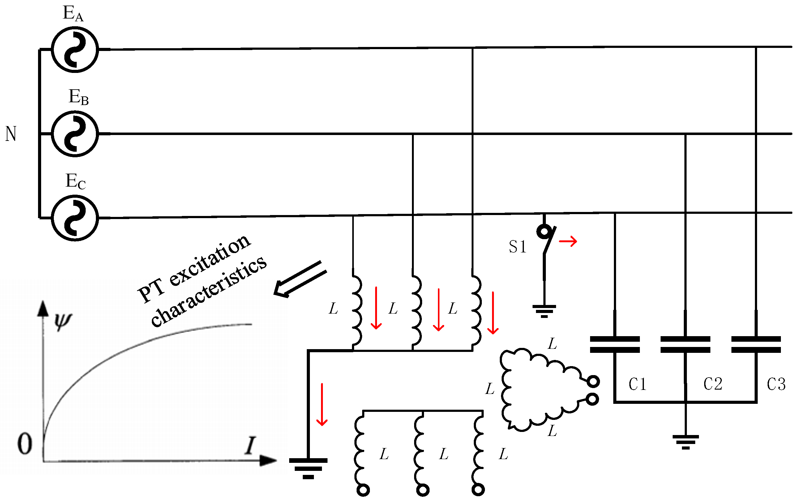Figure 1 illustrates the mechanism by which the clearance of a single-phase ground fault can excite ferroresonance.

A grounded potential transformer (PT) is typically installed to monitor the bus voltage in a neutral ungrounded system. At this time, the only path to ground for the system is through the grounding point of the PT’s primary winding. Owing to the nonlinear magnetization properties inherent in the PT, when switch S1 opens and the single-phase grounding fault clears, the significant charge stored in the non-fault phases A and B during the fault period can only be discharged through the grounding point of the PT’s primary winding, as indicated by the red arrows in the figure. The resulting instantaneous inrush current causes magnetic saturation of the PT, leading to a sharp drop in excitation impedance. Ferroresonance is excited when this impedance matches the earth capacitance parameters. Due to varying degrees of magnetic saturation, the natural oscillation angular frequency of the nonlinear oscillation circuit changes accordingly. Consequently, fundamental frequency, fractional frequency, and high-frequency ferroresonance may occur for the same circuit.

3. Resonance Fault Identification Based on GASF and Improved Cloud Model

3.1. The Principle of SGMD

Based on Takens’ embedding theorem [28], the high-dimensional time series $X=\left\{x_1,x_2,\cdot \cdot \cdot ,x_n\right\}$ can be equivalently reconstructed into a multi-dimensional state space, thereby yielding the reconstructed trajectory matrix $X_{\mathrm{C}}$.

$$X_{\mathrm{c}}=\left[\begin{array}{cccc}{x}_1& x_{1+\tau }& \cdots & x_{1+\left(d-1\right)\tau }\\ ⋮& ⋮& & ⋮\\ x_m& x_{m+\tau }& \cdots & x_{m+\left(d-1\right)\tau }\end{array}\right]$$

(1)

where $\tau$ represents the delay time and d is the embedding dimension. When the embedding dimension and delay time change, the reconstructed trajectory matrix also changes accordingly. This paper employs the power spectral density (PSD) method to configure the aforementioned parameters. Specifically, by analyzing the PSD of the signal, we identify its primary frequency component $f_0$, and let $\tau =1/f_0$. The embedding dimension is determined based on the bandwidth information from the PSD analysis; typically, a wider bandwidth corresponds to a higher embedding dimension. If the maximum peak frequency $f_{\max }$ of time series X’s PSD is identified, and when the normalized frequency is below the threshold of ${10}^{-3}$, the embedding dimension d is set to n/3. The normalization threshold is an empirical coefficient, commonly defined as a percentage of the total PSD energy. Reference [29] demonstrated through simulations that a threshold of ${10}^{-3}$ can effectively remove high-frequency noise while preserving the primary characteristics of the signal. Therefore, this paper adopts a threshold of ${10}^{-3}$. If the threshold requirement is not satisfied, then $d=1.2\times (F_s/f_{\max })$, where Fs denotes the sampling frequency.

Calculate the covariance matrix $A=X_{\mathrm{c}}^T{X}_{\mathrm{c}}$ of the trajectory matrix and then construct the Hamiltonian matrix $M$.

$$M=\left[\begin{array}{cc}A& 0\\ 0& -A^{\mathrm{T}}\end{array}\right]$$

(2)

Let $N=M^2$ and construct the symplectic orthogonal matrix $Q$ via Equation (2).

$$Q^{\mathrm{T}}NQ=\left[\begin{array}{cc}B& R\\ 0& B^{\mathrm{T}}\end{array}\right]$$

(3)

where B is an upper triangular matrix. If the eigenvalue of B is ${\lambda }_1,{\lambda }_2,\cdot \cdot \cdot {\lambda }_d$, then by the properties of the Hamiltonian matrix, the eigenvalue of the covariance matrix A is

$${\sigma }_i=\sqrt{{\lambda }_i} i=1,2,\cdots ,d$$

(4)

To perform symplectic geometry transformation decomposition on matrix $M$, we first construct a real matrix $H$ to replace the symplectic orthogonal matrix $Q$ and set $S=Q^{T}X,Z=QS$. Consequently, the reconstructed trajectory matrix $Z$ can be obtained. The construction process is as follows:

First, the transformation coefficient matrix $S$ is derived from the trajectory matrix and the eigenvectors of the unitary matrix.

$$S_i=Q_i^T{X}^T$$

(5)

The transformation of matrix $S$ yields the reconstructed matrix $Z$.

$$Z_i=Q_i{S}_i$$

(6)

where $Z_i(i=1,2,\cdot \cdot \cdot ,d)$ is the initial single-component matrix. Summing up $Z_i$ as mentioned above will yield the trajectory matrix $Z=Z_1+Z_2+\cdot \cdot \cdot +Z_d$.

If the elements in the matrix ${10}^{-3}$ are $z_{ij}$, where $1\le i\le d,$ then $n=m+(d-1)\tau$, $d^{*}=\min (m,d)$, and $m^{*}=\max (m,d)$ $Y_i(y_1,y_2,\cdot \cdot \cdot ,y_k,\cdot \cdot \cdot ,y_n)$, the reconstructed signal, is determined by Equation (7).

Therefore, the diagonal average transfer matrix is

$$y_k=\left\{\begin{array}{l}{\displaystyle \frac{1}{k}}{\displaystyle \sum _{p=1}^k{z}_{p,k-p+1}^{*}\hspace{0.33em}\hspace{0.33em}\hspace{0.33em}\hspace{0.33em}\hspace{0.33em}\hspace{0.33em}\hspace{0.33em}\hspace{0.33em}\hspace{0.33em}\hspace{0.33em}\hspace{0.33em}\hspace{0.33em}\hspace{0.33em}\hspace{0.33em}\hspace{0.33em}\hspace{0.33em}\hspace{0.33em}\hspace{0.33em}\hspace{0.33em}\hspace{0.33em}1⩽k<d^{*}}\\ {\displaystyle \frac{1}{d^{*}}}{\displaystyle \sum _{p=1}^{d^{*}}{z}_{p,k-p+1}^{*}\hspace{0.33em}\hspace{0.33em}\hspace{0.33em}\hspace{0.33em}\hspace{0.33em}\hspace{0.33em}\hspace{0.33em}\hspace{0.33em}\hspace{0.33em}\hspace{0.33em}\hspace{0.33em}\hspace{0.33em}\hspace{0.33em}\hspace{0.33em}\hspace{0.33em}\hspace{0.33em}\hspace{0.33em}\hspace{0.33em}{d}^{*}⩽k⩽m^{*}}\\ {\displaystyle \frac{1}{n-k+1}}{\displaystyle \sum _{p=k-m^{*}+1}^{n-m^{*}+1}{z}_{p,k-p+1}^{*}\hspace{0.33em}\hspace{0.33em}\hspace{0.33em}\hspace{0.33em}{m}^{*}<k⩽n}\end{array}\right.$$

(7)

where, when $m<d$, $z_{ij}^{*}=z_{ij}$; otherwise,$z_{ij}^{*}=z_{ji}$.

The reconstructed signal $y_i$ is not an independent component and requires periodic similarity comparison. Only components with high reconstruction similarity should be retained. If the first reconstructed component is SGC1, the elements involved in the reconstruction of SGC1 should be removed from matrix Y. The resulting parameter matrix is denoted as g¹. Sum the remaining elements of matrix $G^1$ to obtain $g^1$ and calculate the normalized average variance of the residual signal:

$$NMS{E}^h={\displaystyle \frac{{\displaystyle \sum _{e=1}^n{g}^h}(e)}{{\displaystyle \sum _{e=1}^{n}x}(e)}}$$

(8)

where h represents the number of iterations. When NEME is less than the threshold requirement, the decomposition process ends, and the final decomposition result is obtained.

$$x{(n)}^2={\displaystyle \sum _{h=1}^{N}S}G{C}^h{(n)}^2+g^{(N+1)}(n)$$

(9)

where N is the number of components obtained from the decomposition.

3.2. GASF Coding Principle

The Gramian Angular Field (GAF) is a technique that transforms one-dimensional time series into two-dimensional images through encoding. GAF and time series have a corresponding mapping relationship, which can reveal the periodic characteristics of ferroresonance signals in polar coordinates [30]. The specific process is as follows:

To mitigate the potential bias introduced by the maximum observation on the inner product, the time series $X=\left\{x_1,x_2,\cdot \cdot \cdot ,x_n\right\}$ is first normalized to lie within the interval ([−1, 1]) using the following equation:

$${\tilde{x}}_i={\displaystyle \frac{(x_i-\max (X))+(x_i-\min (X))}{\max (X)-\min (X)}}$$

(10)

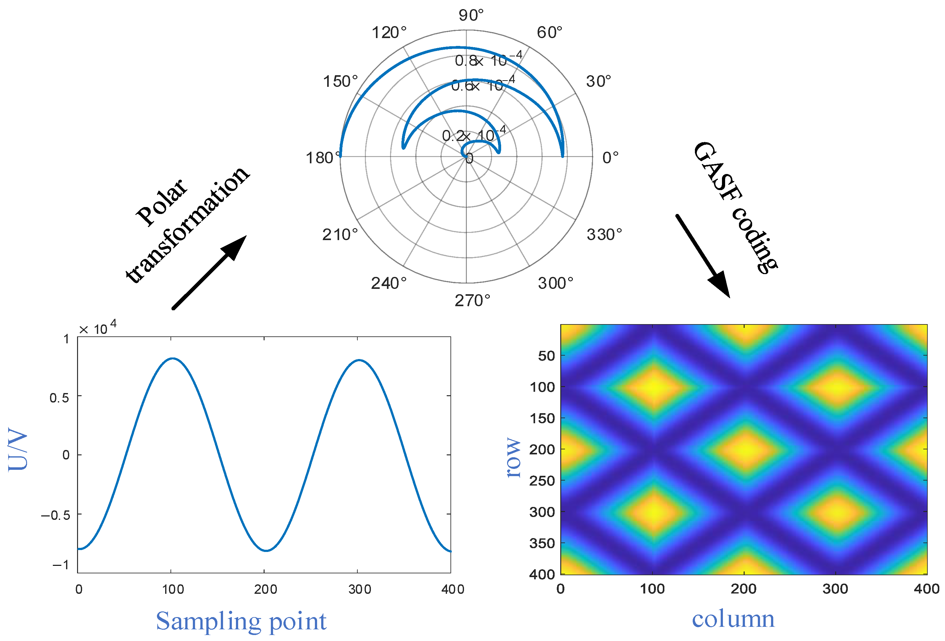
To encode the timestamp as the radius r, convert the scaled values into angles $\phi$, and subsequently transform the normalized time series into the polar coordinate system. The complexity of this conversion is linearly related to the length of the input data sequence; that is, as the length of the data sequence increases, the computational complexity increases accordingly. The calculation formula is

$$\left\{\begin{array}{l}\phi =\arccos ({\tilde{x}}_i)\hspace{0.33em}\hspace{0.33em}\hspace{0.33em}\hspace{0.33em}\hspace{0.33em}\hspace{0.33em}\hspace{0.33em}\hspace{0.33em}\hspace{0.33em}-1\le {\tilde{x}}_i\le 1\\ r={\displaystyle \frac{t_i}{N}}\hspace{0.33em}\hspace{0.33em}\hspace{0.33em}\hspace{0.33em}\hspace{0.33em}\hspace{0.33em}\hspace{0.33em}\hspace{0.33em}\hspace{0.33em}\hspace{0.33em}\hspace{0.33em}\hspace{0.33em}\hspace{0.33em}\hspace{0.33em}\hspace{0.33em}\hspace{0.33em}\hspace{0.33em}\hspace{0.33em}\hspace{0.33em}\hspace{0.33em}\hspace{0.33em}{t}_i\in N\end{array}\right.$$

(11)

where N represents a constant factor in the polar coordinate system, and t denotes the timestamp. As time progresses, the sequence X is mapped to different angles and radii in the polar coordinate system, resulting in distortions among points at various angular positions across the circle. From Equation (11), it can be observed that due to the relationship $-1\le {\tilde{x}}_i\le 1$ and $0\le {\phi }_i\le \pi$, within this interval, the cos$\phi$ function exhibits monotonicity. Therefore, a unique mapping exists for a specific time series. Consequently, GAF can accurately characterize ferroresonance overvoltage signals with nonlinear features.

The GASF is constructed by computing the cumulative angles between each pair of angular points in the polar coordinate system, which allows for the extraction of temporal correlations across varying time intervals [31]. The encoding method of GASF is defined as follows:

$$GASF=\left[\begin{array}{ccc}\cos ({\varphi }_1+{\varphi }_1)& \cdots & \cos ({\varphi }_1+{\varphi }_n)\\ \cos ({\varphi }_2+{\varphi }_1)& \cdots & \cos ({\varphi }_2+{\varphi }_n)\\ ⋮& \cos ({\varphi }_i+{\varphi }_i)& ⋮\\ \cos ({\varphi }_n+{\varphi }_1)& \cdots & \cos ({\varphi }_n+{\varphi }_n)\end{array}\right]={\tilde{X}}^{\prime }\cdot \tilde{X}-\sqrt{I-{{\tilde{X}}^{\prime }}^2}\cdot \sqrt{I-{\tilde{X}}^2}$$

(12)

where $\tilde{X}$ and ${\tilde{X}}^{\prime }$ denote the row vectors of the sequence before and after scaling, I represents the unit row vector, and ${\phi }_i\left\{i=1,2,\cdot \cdot \cdot ,n\right\}$ is the angle between the corresponding vectors.

Following the GAF transformation, various types of ferroresonance overvoltage signals are converted into corresponding GASF matrices, which are $n\times n$-dimensional symmetric matrices. Since each matrix element involves a trigonometric function operation, the computational complexity scales quadratically with the sequence length. Consequently, dimensionality reduction is necessary when the sequence length exceeds 1000. In this study, the input data lengths range from 200 to 400, classifying them as short sequences, thereby resulting in relatively low transformation complexity. Subsequently, by scaling each element in the matrix, a pixel matrix within the range [0, 255] is generated, thereby constructing the Gram image of the ferroresonance signal. The GASF conversion process is illustrated in Figure 2.

3.3. Grey-Level Co-Occurrence Matrix

The GLCM is a widely used technique for extracting texture features from images. It captures comprehensive information about the image’s grey levels across multiple dimensions, including variation amplitude, direction, and spatial intervals between adjacent pixels. Specifically, the GLCM represents the joint probability density of pixel grey-level pairs obtained based on a specified displacement relationship between neighbouring pixels. This matrix characterizes the spatial distribution of grey levels in the image and provides an intuitive representation of the grey-level domain within the spatial domain [32].

If the two-dimensional digital image f(x,y) has a grey level of G and a size of $M\times N$, then the GLCM can be expressed as

$$P(i,j,d,\theta )=g\{(x_1,y_1),(x_2,y_2)\in M\times N|f(x_1,y_1)=i,f(x_2,y_2)=j\}$$

(13)

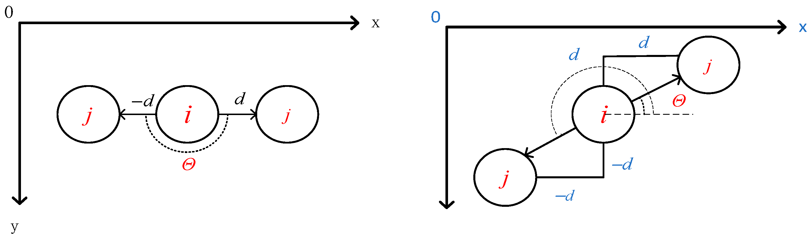
In the formula, P is a G×G matrix, g(x) represents the number of elements in the set, θ is the angle formed by the horizontal coordinate axis and two pixel points, and d is the distance between the pixel points. The values of d and θ determine the pixel direction of the GLCM. The illustration of the pixel direction is shown in Figure 3.

Let $P(i,j,d,\theta )$ represent the element at the i-th row and j-th column of the GLCM. By traversing the entire image and recording the occurrence frequency of each grey-level pair (i, j) while keeping the displacement relationship between pixel pairs unchanged, the following matrix can be constructed:

$$P_d=\left[\begin{array}{cccccc}{P}_d(0,0)& P_d(0,1)& \cdots & P_d(0,j)& \cdots & P_d(0,G-1)\\ P_d(1,0)& P_d(1,1)& \cdots & P_d(1,j)& \cdots & P_d(1,G-1)\\ \cdots & \cdots & \cdots & \cdots & \cdots & \cdots \\ P_d(i,0)& P_d(i,1)& \cdots & P_d(i,j)& \cdots & P_d(i,G-1)\\ \cdots & \cdots & \cdots & \cdots & \cdots & \cdots \\ P_d(G-1,0)& P_d(G-1,1)& \cdots & P_d(G-1,j)& \cdots & P_d(G-1,G-1)\end{array}\right]$$

(14)

In this paper, d = 2 and θ = 0° are selected; then, the point coordinate values in the GLCM can be expressed as:

$$P(f(x_1,y_1),f(x_2,y_2),2,0^{°})={\displaystyle \sum \{[f(}{x}_1,y_1),f(x_2,y_2)]\mid x_2-x_1=0,\left|y_2-y_1\right|=2\}$$

(15)

where we let $\mathrm{\Sigma }$ represent the total number of elements that meet the constraint conditions.

To more effectively characterize the texture information of images, this study employs the second-order statistics derived from the GLCM to describe image texture quantitatively. Second-order statistical measures commonly include entropy, contrast, angular second moment, and homogeneity. This paper selects entropy, angular second moment, and contrast as the key texture feature values for image analysis.

3.4. Improved Cloud Model Theory

3.4.1. Principles of Cloud Model

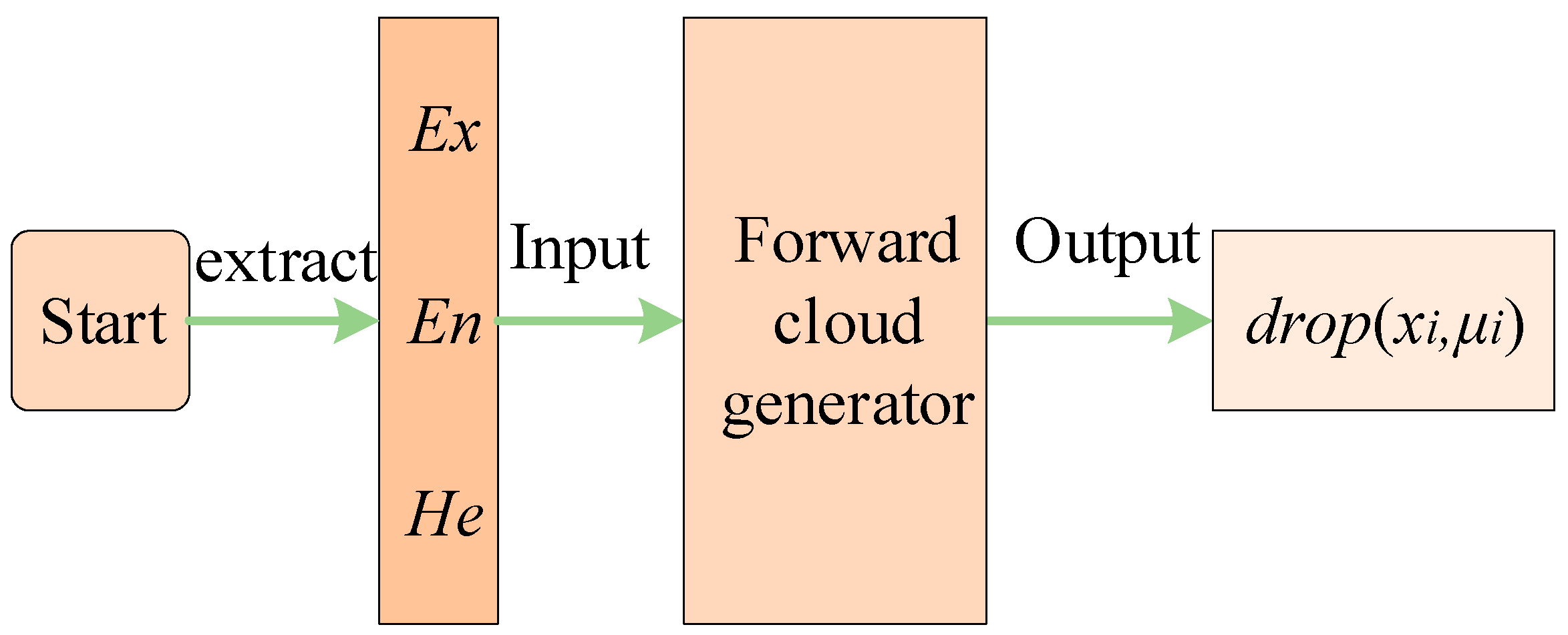
The cloud model, derived from fuzzy set theory and probability theory, facilitates the transformation of uncertainty between quantitative data and qualitative concepts. Assume that U is a dataset and $U=\left\{x\right\}$ is an argument domain; let U denote the universe of discourse and A be a fuzzy set within U. For any element x in A, x represents a random realization of A, with $\mu (x)\in [0,1]$ indicating its membership degree to A. The mapping distribution of A in the numerical domain space of U is referred to as a cloud. In this context, the membership degree of element x to a qualitative concept in the universe of discourse U is represented by a cloud droplet $drop(x_i,{\mu }_i)$.

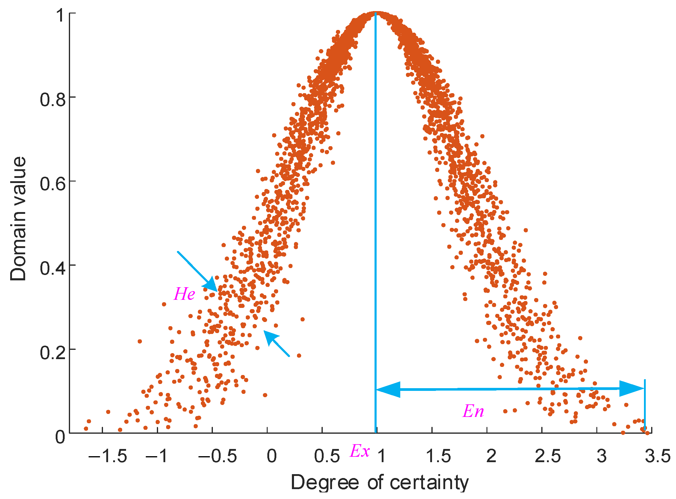
In the cloud model framework, two distinct types of generators are employed: the forward cloud generator and the reverse cloud generator. The reverse cloud generator, the standard cloud generator, is utilized to quantify the digital characteristics of cloud droplets. Conversely, the forward cloud generator transforms input data into a predefined number of cloud droplets. These generators characterize the cloud model using three key parameters: entropy (En), expectation (Ex), and hyper-entropy (He). Expectation denotes the central tendency of cloud droplet distribution within the domain space. The entropy characterizes the fuzziness and randomness of the observed data, reflecting the extent to which the fuzzy concept within the domain space encompasses cloud droplets. Hyper-entropy serves as a measure of entropy, indicating both the thickness of the cloud layer and the dispersion of cloud droplets [33]. The traditional cloud model relies on parameters such as Ex, En, and He, which can only characterize the overall distribution of input data but struggle to capture the spatial distribution features of images. This paper proposes an improved cloud model method that incorporates image texture features (entropy, angular second moment, and contrast) into the cloud generator as feature parameters. This approach leverages the intrinsic relationship between these texture features and resonance signals. By doing so, it establishes a bridge between the spatial distribution characteristics of resonance signals and the uncertainty transformation in the cloud model, thereby achieving the conversion from GLCM quantitative data to the qualitative concept of resonance types. The mapping relationships of the relevant parameters are detailed in Equations (16)–(18). Figure 4 illustrates the relationship between these characteristic parameters and the cloud droplets.

Sample entropy calculation formula:

$$E_{\mathrm{x}}=\overline{X}={\displaystyle \frac{1}{n}}{\displaystyle \sum _{i=1}^n{x}_i}$$

(16)

Entropy, which is the mean value of the elements in the GLCM, reflects the amount of information and the complexity of the texture features in an image. The higher the entropy value, the richer and more complex the texture information in the image.

The formula for calculating the angular second moment is

$$E_n=f_1={\displaystyle \sum _{i=1}^G{\displaystyle \sum _{j=1}^G[}}\widehat{P}(i,j){]}^2$$

(17)

where $\stackrel{⌢}{P}(i,j)$ is the normalized GLCM element, representing the probability of grey value occurrence.

The angular second moment reflects the uniformity of image texture and the consistency of grey-level distribution. Higher values of this statistic indicate more regular textures and more uniform grey-level distributions in the image.

Contrast calculation formula:

$$H_{\mathrm{e}}=f_2={\displaystyle \sum _{n=0}^{G-1}{n}^2}{\displaystyle \sum _{i=1}^G{\displaystyle \sum _{j=1}^G\widehat{P}}}(i,j)$$

(18)

where $n=\left|i-j\right|$, $n^2$ represents the square of the difference in grey level.

Contrast reflects the depth and sharpness of the image texture. The sharper the image, the higher the contrast.

The input parameters of the cloud model, namely entropy, contrast, and angular second moment, serve as key bridges for transforming uncertainty from the quantitative data of GLCM to the qualitative concept of resonance types. These parameters effectively quantify the texture features of reconstructed images derived from ferroresonance signals, thereby significantly enhancing the accuracy and robustness of type recognition.

3.4.2. Forward Cloud Generator

(1)

Generate a normal random number with an expected value of En and a variance of $H{e}^2$.

$$E_{nn}=\mathrm{norm}(E_n,H_e^2)$$

(19)

(2)

Generate a normal random number with an expected value of Ex and a variance of ${E_{nn}}^2$.

$$x_i=norm(Ex,E_{nn}^2)x_i=norm(Ex,E_{nn}^2)$$

(20)

(3)

Calculate the sample certainty.

$$\mu (x_i)=\exp [-{\displaystyle \frac{{(x-E_x)}^2}{2E_{nn}^2}}]$$

(21)

(4)

Sample x and certainty degree constitute a cloud droplet. Repeat Equations (19)–(21) until a sufficient number of cloud droplets are generated. An example of the forward cloud generator is shown in Figure 5.

3.4.3. Cloud Model Membership Degree Measurement

(1)

Generate the cloud droplets of the index cloud and the cloud to be tested.

$$\left\{\begin{array}{l}Dro{p}^1(i)=\mathrm{Coud}(E{x}^1,E{n}^1,H{e}^1,n)\\ Dro{p}^2(i)=\mathrm{Coud}(E{x}^1,E{n}^1,H{e}^1,n)\end{array}\right.$$

(22)

(2)

Sort the cloud droplets.

$$\left\{\begin{array}{l}\mathrm{Sort}(D{\mathrm{rop}}^1)\\ \mathrm{Sort}(D{\mathrm{rop}}^2)\end{array}\right.$$

(23)

(3)

Screen out cloud droplets within the range of $\left[Ex-3En,Ex+3En\right]$.

(4)

Calculate the Euclidean distance between two cloud droplets after the screening. If it meets the set threshold requirement, it can be considered that the two have similarity.

$$\left\{\begin{array}{l}dis(i)=\sqrt{{(x1(i)-x2(i))}^2+{(y1(i)-y2(i))}^2}\\ sim=mean(dis)\end{array}\right.$$

(24)

where dis represents the Euclidean distance between two cloud droplets; sim indicates similarity.

3.5. Identification Process of Ferroresonance Faults

The fault identification process of ferroresonance based on GASF and the improved cloud model is as follows:

(1)

Obtain the overvoltage time series, decompose the original sequence using the SGMD algorithm to extract the dominant mode of the signal, and reconstruct the signal.

(2)

Map the one-dimensional reconstructed overvoltage sequence into a two-dimensional image using GASF and perform grayscale processing on the encoded image.

(3)

Extract the texture features of GASF images for different types of ferroresonance through the GLCM and establish a set of texture feature parameters.

(4)

Use the standard cloud generator to construct the cloud distribution model of the texture feature parameters for the reconstructed GASF images of different resonance types. Repeat steps 1–3 to generate the standard cloud model of the signal to be identified using the forward cloud generator.

(5)

Calculate the membership degree between the standard cloud of the signal to be identified and the cloud model library of resonance type indicators, and determine the type of ferroresonance based on this.

To facilitate a clearer understanding of the algorithm flow, the pseudo-code of the proposed method is presented below (Algorithm 1).

Algorithm 1: Ferroresonance fault identification

Input: Overvoltage signal Output: Resonance type begin # Step 1: SGMD Denoising and Signal Reconstruction denoised_signal = SGMD_denoise(overvoltage_signal) reconstructed_signal = reconstruct(denoised_signal, selected_components) # Step 2: GASF Image Transformation gasf_image = GASF_transform(reconstructed_signal) # Step 3: GLCM Texture Feature Extraction glcm = compute_GLCM(gasf_image) texture_features = {   ‘entropy’: calculate_GLCM_entropy(glcm),   ‘ASM’: calculate_GLCM_ASM(glcm),   ‘contrast’: calculate_GLCM_contrast(glcm)} # Step 4: Cloud Model Generation for Resonance Types cloud_models = {} for resonance_type IN training_data:   model_features = aggregate_features(training_data[resonance_type])   cloud_models[resonance_type] = generate_cloud_model(model_features) end for # Step 5: Membership Calculation and Type Identification test_cloud = build_standard_cloud(texture_features) max_membership = 95 # Assuming percentage representation (i.e., 95%) identified_type = None for resonance_type IN cloud_models:   membership_score = compute_membership(test_cloud, cloud_models [resonance   _type])   if membership_score > max_membership:      identified_type = resonance_type   end if end for return identified_type end

4. Simulation Verification

4.1. Simulation Parameter Settings

To verify the feasibility of the method, as in Algorithm 1. A 110/10 kV distribution system ferroresonance simulation model was constructed using EMTP-ATP, as illustrated in Figure 1. The identification scheme was validated through simulation. The excitation characteristic parameters of the PT are provided in

Table 1. PT excitation parameters.

I/mA	$\mathit{\varphi }$/Wb	I/mA	$\mathit{\varphi }$/Wb
1.5	5.09	11.62	38.32
2.5	12.77	18.83	47.17
5.3	24.15	28.10	52.14
7.6	30.51	44.11	56.62

. The three-phase voltages at the 110 kV level are

$$\left\{\begin{array}{l}{E}_A=U_{\mathrm{m}}\sin (\omega t+{\theta }_0+0^{°})\\ E_B=U_{\mathrm{m}}\sin (\omega t+{\theta }_0-{120}^{°})\\ E_C=U_{\mathrm{m}}\sin (\omega t+{\theta }_0+{120}^{°})\end{array}\right.$$

(25)

where $U_{\mathrm{m}}=110000\sqrt{2}/\sqrt{3}=89.8146\hspace{0.33em}\mathrm{k}V$; ${\theta }_0$ is the initial phase angle of the power source.

4.2. GASF-Encoded Images Based on SGMD Reconstruction

4.2.1. Time Series of Ferroresonance Overvoltage

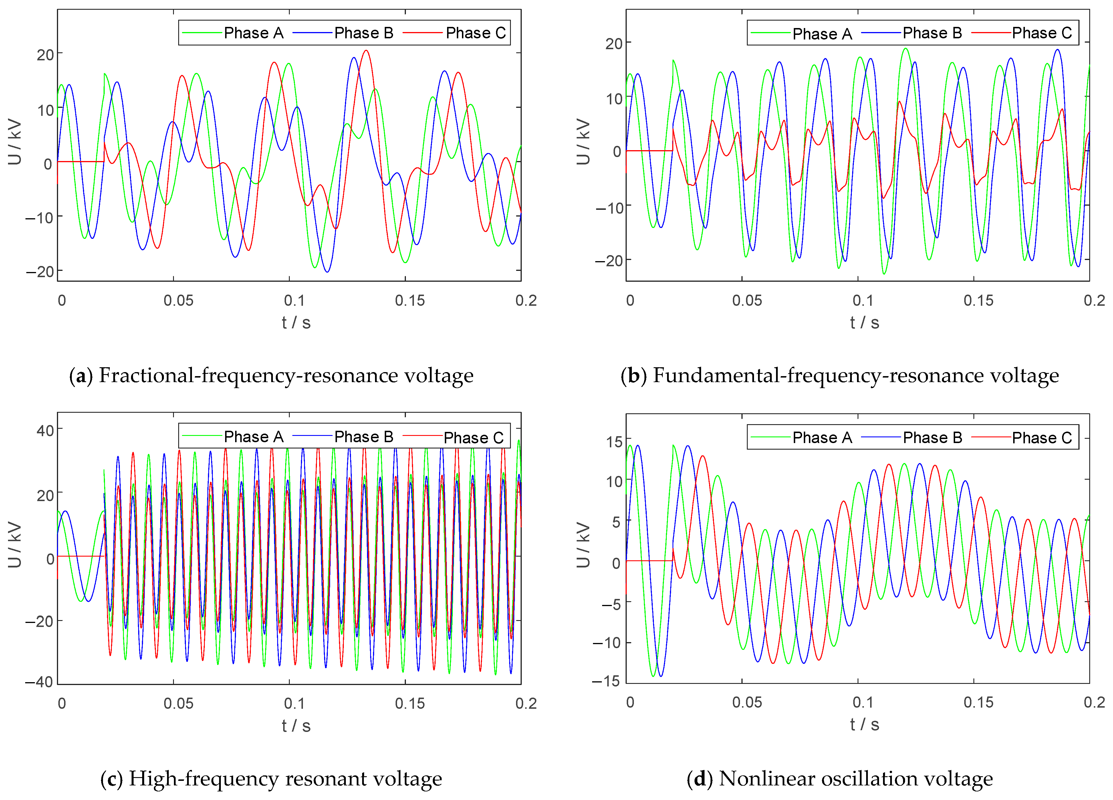
As shown in Figure 6, different ferroresonances exhibit distinct time–frequency characteristics on the same time scale. In the case of fractional frequency resonance, the resonant frequency is a fraction of the power frequency. At this point, the overvoltage level is relatively low, but the overcurrent level is high, which can easily lead to the burnout of the PT. In the fundamental-frequency-resonance state, the resonant frequency matches the power frequency, and the overvoltage level often exceeds the line voltage. In contrast, the overcurrent level is relatively lower compared to fractional frequency resonance. In the high-frequency-resonance state, the resonant frequency is an integer multiple of the power frequency. At this point, the overvoltage level can reach 3 to 4 times the rated voltage, posing a serious threat to the insulation performance of electrical equipment. In contrast, the overcurrent level is usually low and generally does not affect the safe operation of the PT. In the nonlinear oscillation state, the dominant resonant frequency is the fundamental frequency, with additional low-frequency components present. The waveform exhibits nonlinear changes on the time scale, and at this point, the overcurrent level can reach 2 to 3 times the fuse current of the PT.

4.2.2. Time Series Reconstruction Characteristics of Ferroresonance Overvoltage

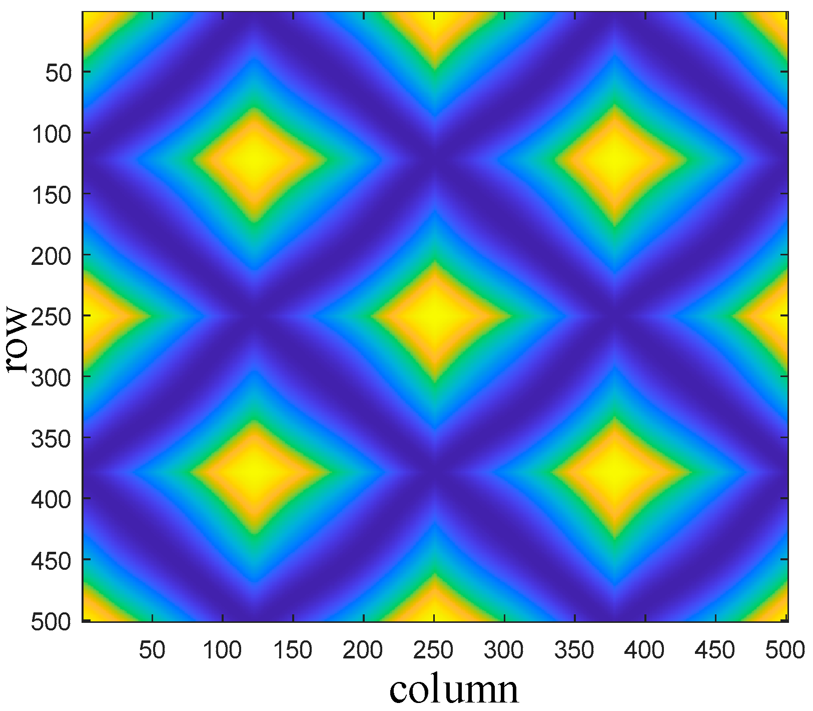
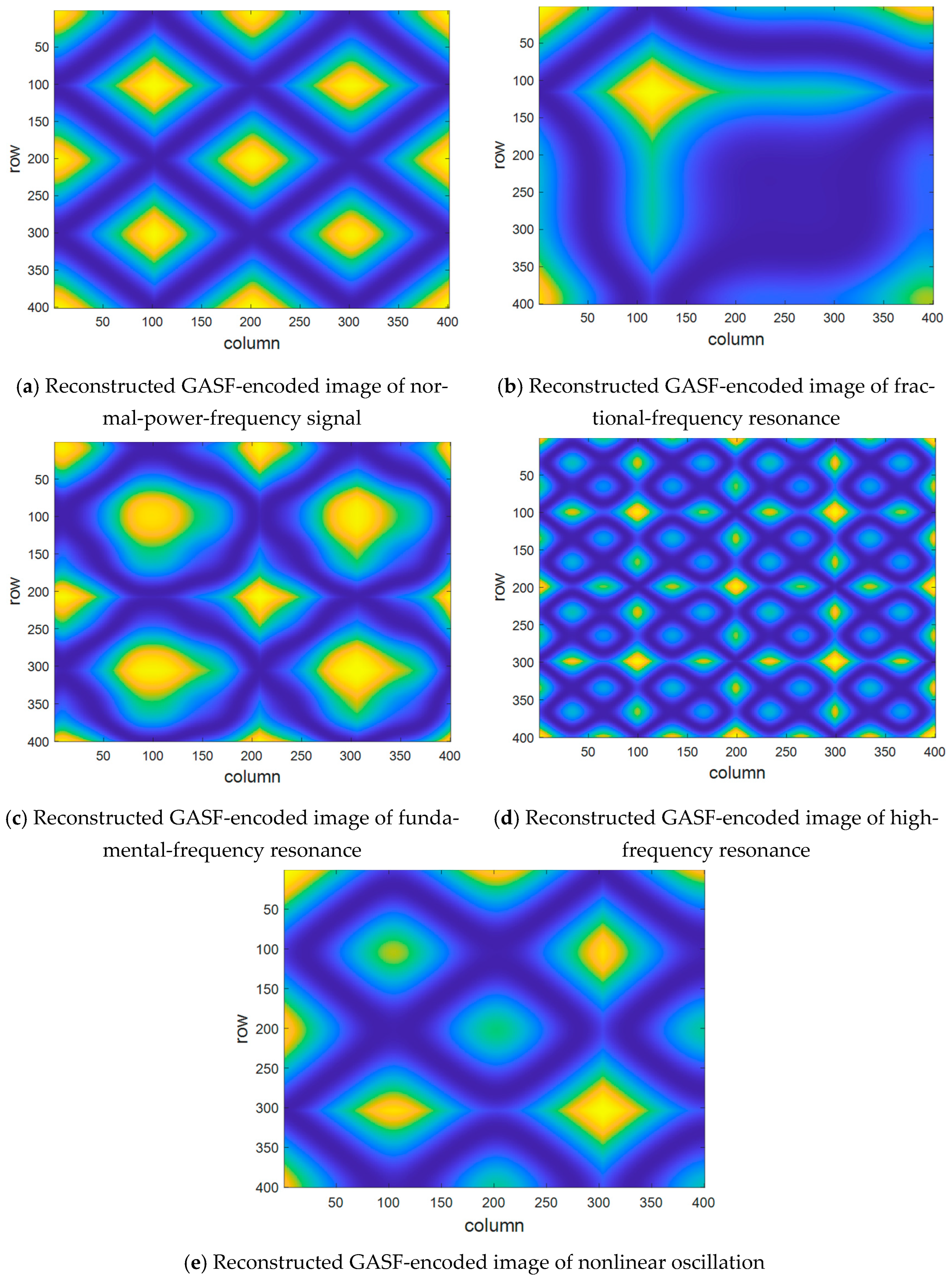
The GASF transformation encodes one-dimensional ferroresonance signals into two-dimensional feature matrices corresponding to the time series. Therefore, GASF can reveal the chaotic characteristics of ferroresonance signals in polar coordinates. Taking the ferroresonance shown in Figure 6 as an example (with a sampling frequency of 10 kHz), the GASF-encoded images of the ferroresonance for two power-frequency cycles obtained by the method proposed in this paper are as follows.

As illustrated in Figure 7, GASF-encoded images of different types of ferroresonance signals exhibit distinct texture features. The encoded image of the standard-power-frequency signal displays high symmetry, with each phase point cluster in an axisymmetric state and the groove depths evenly distributed. In the fractional-frequency-resonance encoded image, each phase point cluster’s size is slightly smaller than the standard-power-frequency signal, and the number of phase point centre clusters also decreases accordingly. The fundamental-frequency-resonance encoded image similarly distributes phase point clusters to the standard-power-frequency encoded image. However, the phase points within each cluster are randomly distributed and no longer symmetrical, with unevenly distributed groove depths. The high-frequency-resonance encoded image contains more phase point clusters, but each cluster has weaker energy, resulting in more complex texture features. The nonlinear oscillation encoded image shows a symmetrical distribution of phase point clusters and evenly distributed groove depths, but the overall image lacks global symmetry.

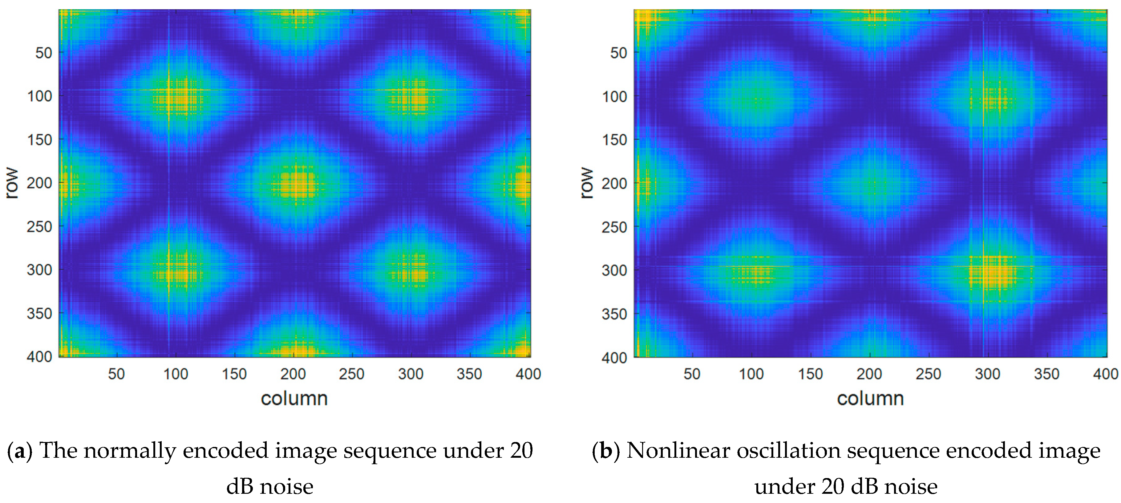
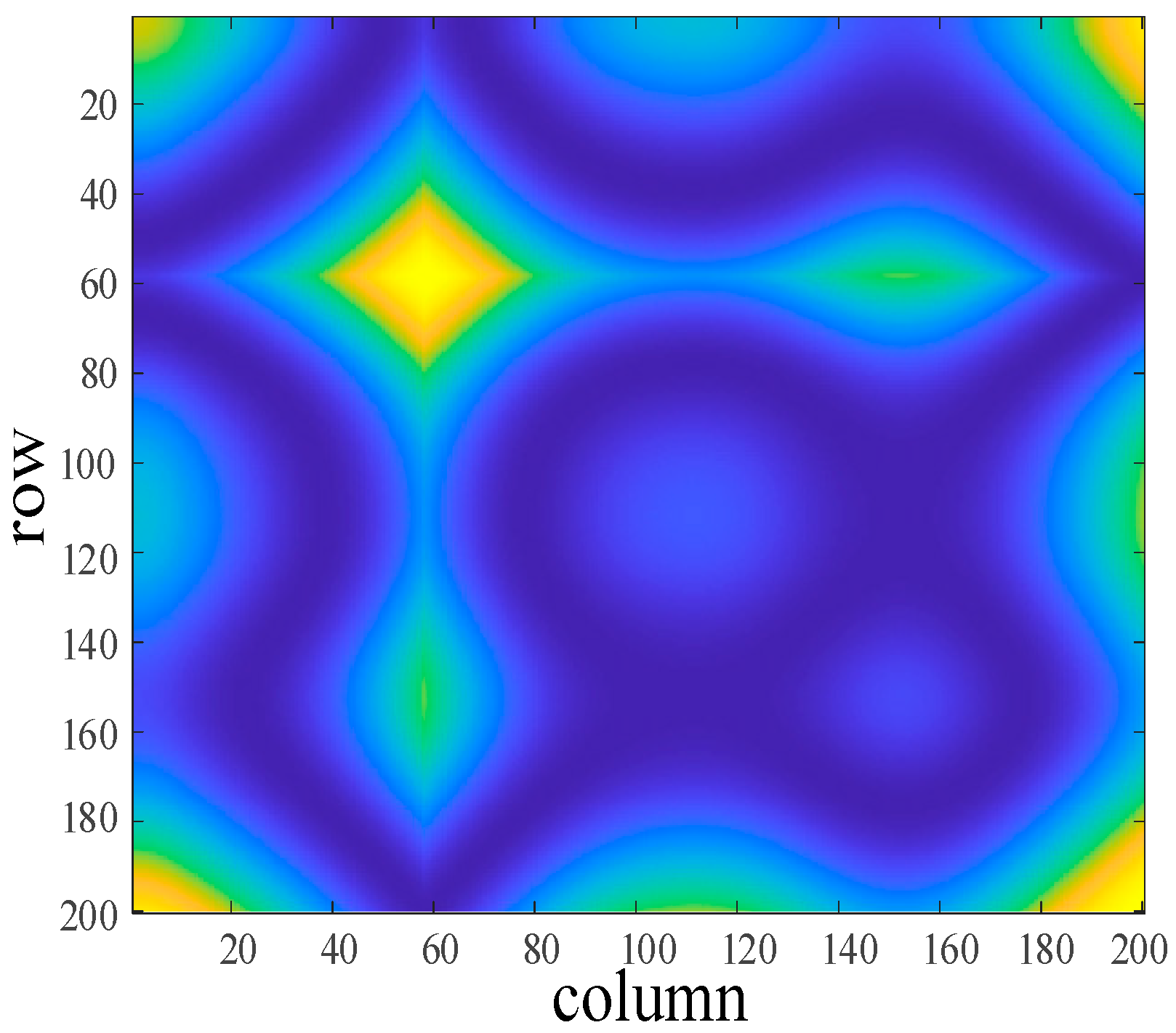
GASF is a technique that transforms one-dimensional time series into two-dimensional images through encoding, maintaining a corresponding mapping relationship between the GASF image and the time series. Noise can obscure the evolution information of moving points. To verify the impact of noise on GASF-encoded images, we use the normal sequence and the nonlinear oscillation sequence from Figure 6 as examples. After adding 20 dB noise, the encoded images are shown in Figure 8.

As shown in Figure 8, the coarseness of texture, the distribution of grey levels, and the depth of grooves in the GASF-encoded image are significantly different under the influence of noise compared to the noise-free condition. Ignoring the impact of noise on the texture features can lead to inaccurate extraction of these features from the GASF-encoded image of ferroresonance signals. Therefore, when mapping a time series to a multi-dimensional space to describe the evolution information of moving points, it is essential to eliminate noise interference.

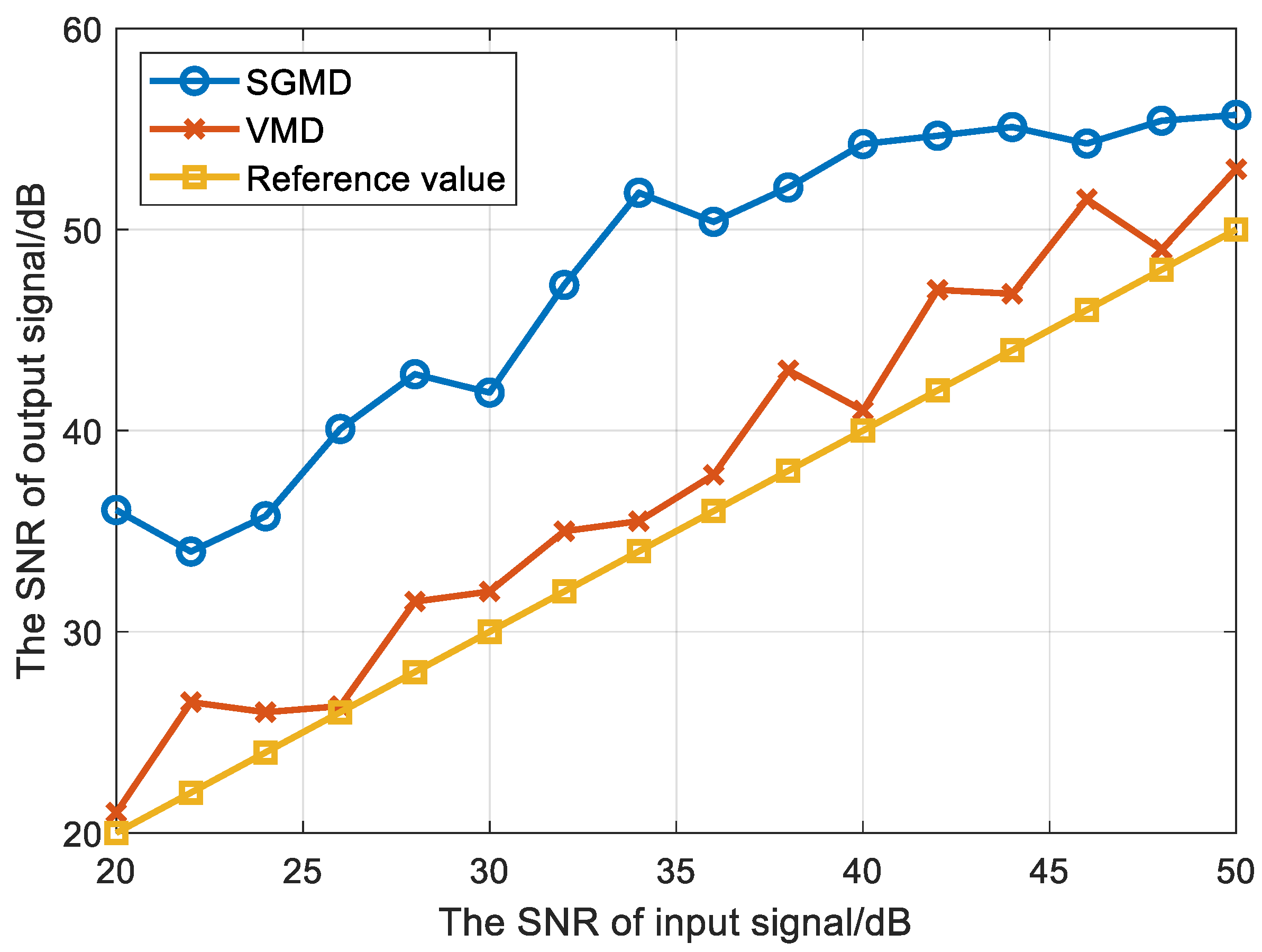
To verify the denoising performance of the SGMD algorithm, we introduced Gaussian white noise with signal-to-noise ratios (SNRs) ranging from 20 to 50 dB into the normal sequence signal and conducted a comparative analysis with the VMD algorithm. The SNR curves after denoising are presented in Figure 9. Here, SNR = 10 × log10(signal power/noise power). A larger SNR indicates that the signal noise is smaller and the noise reduction effect is more obvious.

As illustrated in Figure 9, the SNR after noise reduction using the VMD method remains very close to the pre-noise reduction reference value, indicating that this method has limited effectiveness in reducing noise. The decomposed signal still contains a significant amount of noise components, which may substantially interfere with the accuracy of resonance identification. In contrast, the SGMD method demonstrates more stable and superior noise reduction performance. Within the SNR range of 20 to 35 dB, its noise reduction performance exhibits a linear upward trend and significantly outperforms the VMD method. When the SNR exceeds 36 dB, the noise reduction effect of the SGMD method stabilizes above 50 dB. At this point, the noise content is low and will not affect the texture features of the reconstructed image. Overall, the SGMD method provides better noise reduction and can more accurately reveal the evolution information within the resonance signal.

4.3. Analysis of Texture Features in GASF Images of Ferroresonance

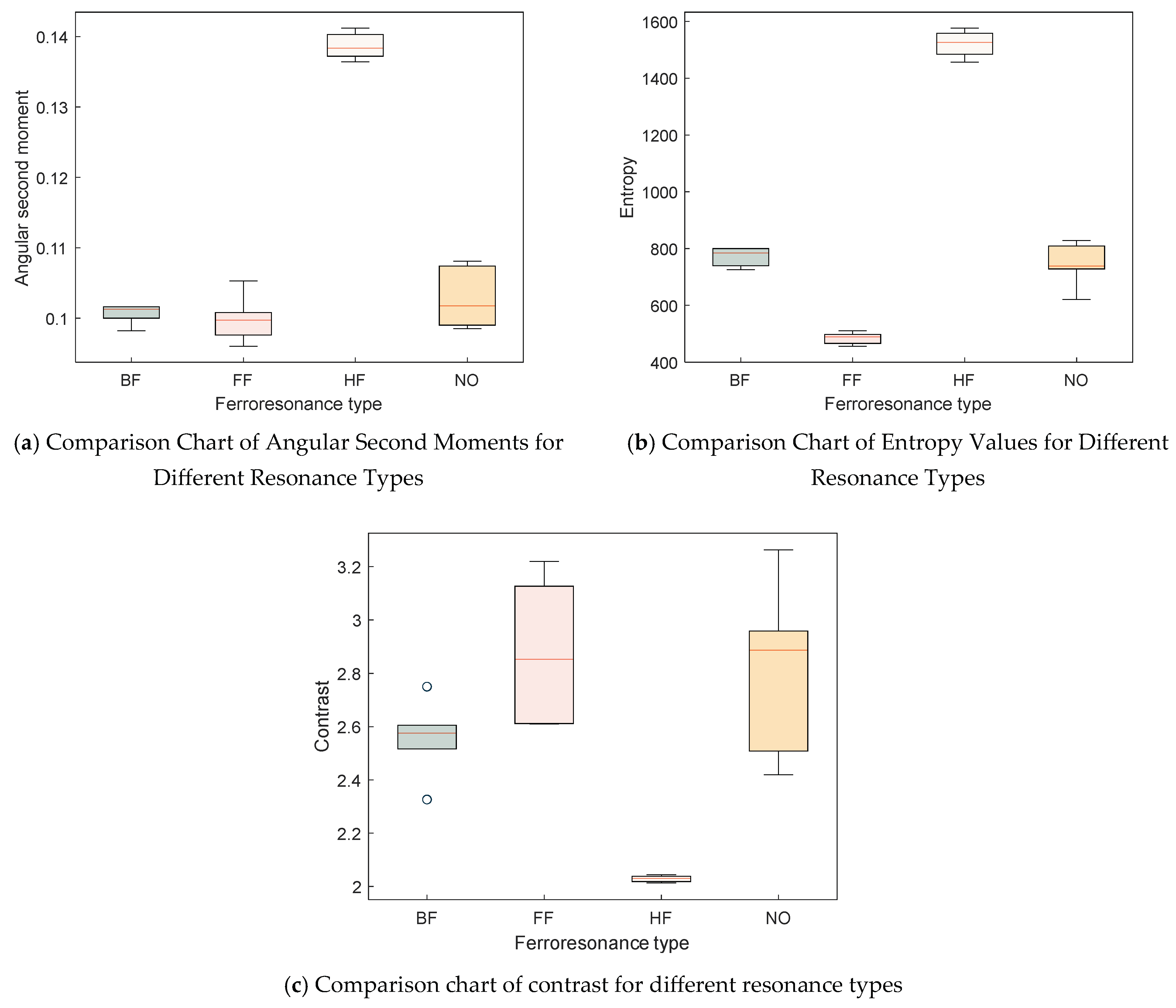
This paper employs the GLCM to extract the spatial mapping relationships of each phase point in the two-dimensional GASF-encoded images to quantitatively describe the texture features of the time series reconstruction images of ferroresonance overvoltage. The following data represent the texture features extracted from six characteristic period resonance signal-encoded images using GLCM. These features include entropy, contrast, and angular second moment, and the characteristic parameters of fractional frequency (FF), fundamental (base) frequency (BF), high frequency (HF), and nonlinear oscillation (NO) are shown in Figure 10.

The angular second moment reflects the coarseness of image texture and the uniformity of grey-level distribution. Figure 10a shows that the angular second moment value of the high-frequency-resonance GASF-encoded image is relatively large, indicating a more uniform grey-level distribution. In contrast, the angular second moment values of fundamental-frequency-resonance images exhibit relatively concentrated changes, suggesting that the fluctuation range within each period is relatively small. The angular second moment changes for the other two resonances are more significant, indicating notable differences in texture coarseness and grey-level distribution uniformity between these two resonant GASF-encoded images.

The entropy value reflects the amount of information in the image texture features and the complexity of the texture. As shown in Figure 10b, the entropy value of the high-frequency-resonance image is the highest, indicating higher texture complexity. Conversely, the entropy value of the fractional-frequency-resonance image is the lowest, indicating less information content in its texture features. Due to the significant differences in entropy values among different resonance types, entropy can serve as an important feature parameter for distinguishing various resonance types.

The contrast reflects the depth of texture grooves and the clarity of the image. Figure 10c shows that the phase point clusters in the high-frequency-resonance GASF-encoded image are distributed uniformly, with relatively uniform groove depths, resulting in lower contrast. In contrast, the groove depths in the fundamental-frequency-resonance GASF-encoded image are unevenly distributed, leading to higher contrast. For nonlinear oscillation and fractional-frequency-resonance GASF-encoded images, the phase point clusters are not symmetrically distributed overall, and compared to the fundamental-frequency-resonance image, they have fewer phase point clusters. Therefore, their contrasts are relatively higher.

In summary, the image texture feature parameters extracted from the GLCM for different types of resonances, such as entropy, contrast, and angular second moment, exhibit significant differences and follow certain patterns. Therefore, different types of ferroresonances can be effectively identified based on the variation patterns of these feature parameters. To quantitatively represent the differences among these feature parameters, the mean values of the six characteristic period feature parameters shown in Figure 9 are used as the feature values to characterize the texture features under different resonance types. The relevant feature value parameters are detailed in

Table 2. Texture feature values of grey-level co-occurrence matrix.

Types	Entropy	Angular Second Moment	Contrast
Normal state	927.23	0.0807	4.399
Fractional frequency	487.36	0.0979	3.1422
Fundamental frequency	923.08	0.0799	2.5265
High frequency	1514	0.1259	3.342
Nonlinear oscillation	733.34	0.0856	5.493

.

As shown in Table 2, the entropy values of different resonance types exhibit significant variation. The entropy values for normal sequences (927.23) and fundamental-frequency resonance (923.08) are relatively high, while those for fractional-frequency resonance (487.36) and nonlinear oscillation resonance (733.34) are notably lower. The entropy value for high-frequency resonance (1514) is the highest, significantly exceeding other types, indicating substantial differences in image complexity among the various resonance types.

In terms of the angular second moment, the value for fundamental-frequency resonance is the lowest (0.0799), whereas that for high-frequency resonance is the highest (0.1259). The angular second moment values for the remaining types—fractional frequency (0.0979), normal (0.0807), and nonlinear oscillation (0.0856)—are relatively close. This suggests that the angular second moment varies less across different resonance types, with only high-frequency resonance showing a more pronounced increase.

In terms of contrast, nonlinear oscillation (5.493) exhibits the highest value, far surpassing other types. Normal resonance (4.399) and high-frequency resonance (3.342) have relatively high contrast, indicating distinct variations in the depth of grooves in their images. In contrast, fractional-frequency resonance (3.1422) and fundamental-frequency resonance (2.5265) have lower contrast, suggesting more moderate variations in the depth of grooves. Overall, the contrast differences among different resonance types reflect the intensity of depth variations in the reconstructed resonance images, from weakest to strongest: fundamental frequency, fractional frequency, high frequency, normal, and nonlinear oscillation.

In summary, entropy, angular second moment, and contrast display clear patterns across different resonance types. By inputting these feature parameters into the cloud model, we can achieve an uncertainty transformation between quantitative data and the qualitative concept of resonance types, thereby enabling accurate identification of resonance types.

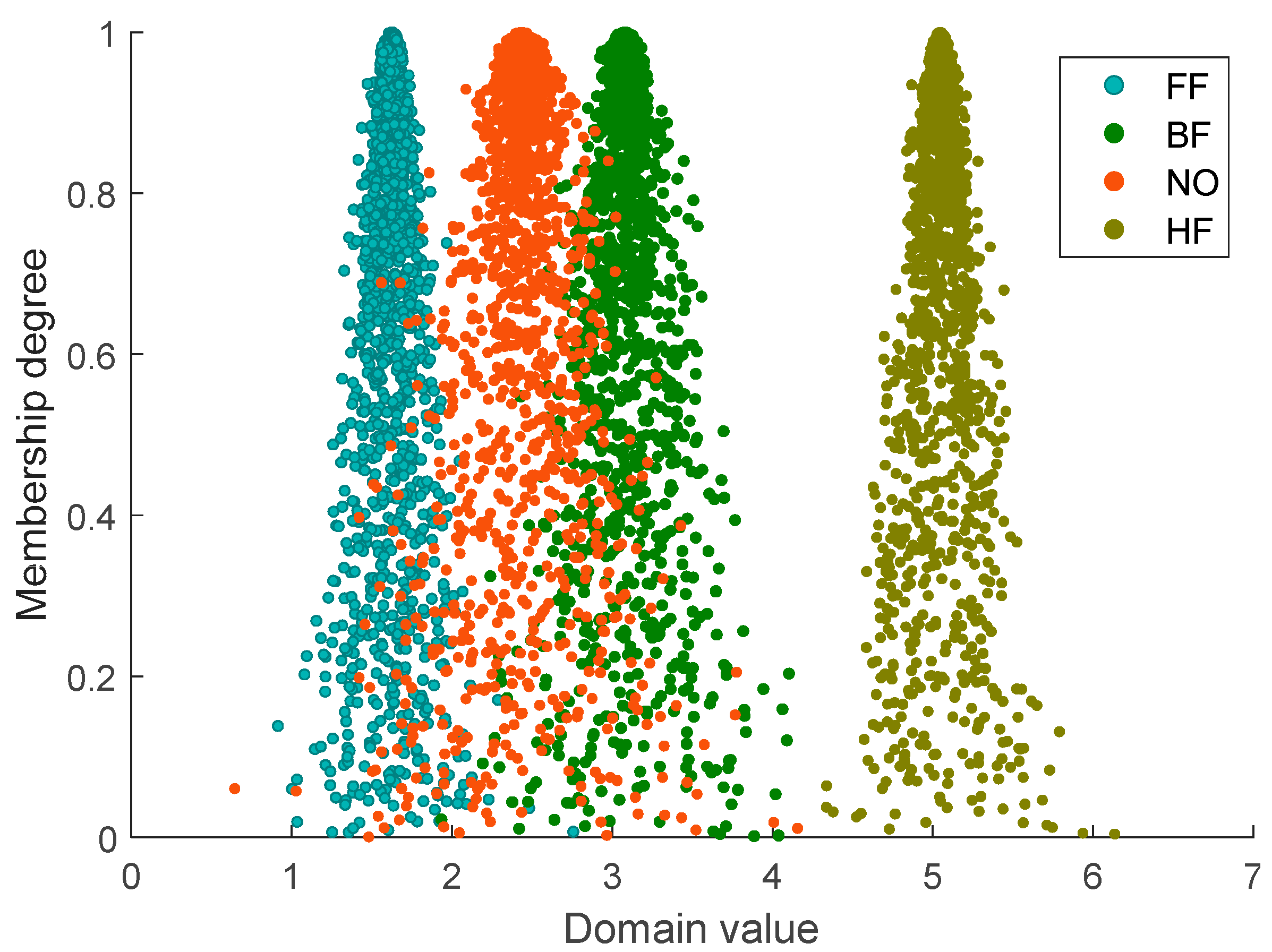
Cloud distribution models of texture feature parameters of reconstructed GASF images of different resonance types were established using the standard cloud generator, as shown in Figure 11. The texture feature parameters are derived from the GLCM of the reconstructed image using Equations (16)–(18). These extracted texture feature values serve as the input parameters for the cloud model. A sufficient number of cloud droplets are then generated via Equations (19)–(21), and the collection of these cloud droplets constitutes the cloud model.

4.4. Comparative Verification

Through the analysis in the Introduction Section, we summarize the limitations of existing resonance identification methods, and the summary is shown in

Table 3. Comparison of limitations of different methods.

Method Types	Extracted Features	Threshold Setting	Misjudgment Rate	Identification Rate
SST	Time-domain and frequency-domain information	Threshold setting is difficult due to the interference of power-frequency signals.	Moderate	Moderate
VMD	Frequency-domain information	Threshold setting is difficult due to the interference of power-frequency signals.	High	Relatively fast
SVM	Time-domain and frequency-domain information	It does not involve threshold setting, but requires a large number of samples for data training.	Low	Relatively low
PSR	Reconstruction of attractor phase plane trajectory characteristics	Threshold setting is imperfect due to noise interference.	High	Fast
Proposed method	GASF encodes image texture features	The SGMD is adopted for noise reduction processing, and the feature extraction is not disturbed by noise. The cloud model rate of belonging is used for resonance identification, avoiding the problem of threshold setting.	Low	Fast

.

As shown in Table 3, the proposed method first uses SGMD to denoise the sequence, thereby ensuring the uniqueness of the mapping relationship between the GASF image and the time series. Secondly, it performs resonance identification by extracting the texture features of the GASF image, effectively avoiding the interference of the signal’s frequency-domain features. Finally, it uses the cloud model to achieve the uncertainty transformation from the quantitative data of GLCM to the qualitative concept of resonance types. This not only avoids the threshold-setting problem but also reduces the reliance on a large amount of sample data, thus having a lower misjudgment rate and a faster identification speed.

To verify the accuracy of the proposed method, we conducted validation using the EMTP-ATP ferroresonance simulation data constructed above under noisy conditions. The simulation results are presented in

Table 4. Results of ferroresonance signal identification.

Noise (SNR)	Series	VMD	Phase Space Reconstruction (PSR)		Proposed Method
			Calculation Criterion	Reference Criterion
50 dB	1	Fractional frequency	0020	0020	Fractional frequency
	2	/	1111	1211	Fundamental frequency
	3	High frequency	0102	0002	High frequency
	4	/	0100	0100	Nonlinear oscillation
30 dB	1	Fractional frequency	0020	0020	Fractional frequency
	2	/	1011	1211	Fundamental frequency
	3	High frequency	0102	0002	High frequency
	4	/	0100	0100	Nonlinear oscillation
20 dB	1	Fractional frequency	0020	0020	Fractional frequency
	2	/	1011	1211	Fundamental frequency
	3	High frequency	0102	0002	High frequency
	4	/	0000	0100	Nonlinear oscillation
0 dB	1	Fractional frequency	0020	0020	Fractional frequency
	2	/	1211	1211	Fundamental frequency
	3	High frequency	0002	0002	High frequency
	4	/	0100	0100	Nonlinear oscillation

. For comparative validation, we employed the frequency-domain identification method VMD and the phase space reconstruction method based on the characteristics of the reconstructed attractor phase plane trajectory. The PSR method includes four evaluation metrics: point distribution factor, correlation dimension, centre distance, and radius vector offset. Each metric corresponds to a reference criterion derived from the resonance type criteria proposed in [31]. By comparing the calculated criteria with the reference criteria, the resonance type can be determined. The calculation rules for the criteria are as follows: when the deviation of the feature quantity from the normal state is within ±10%, the value is set to 1; when the deviation exceeds 10%, the value is set to 2; and when the deviation is less than -10%, the value is set to 0.

As shown in Table 4, in the absence of noise, the VMD method based on frequency-domain identification can accurately identify fractional-frequency resonance and high-frequency resonance. However, due to the presence of fundamental-frequency components in nonlinear oscillations, this method cannot effectively distinguish between fundamental-frequency resonance and nonlinear oscillations. The PSR identification method identifies resonances by extracting the attribute and geometric features of the reconstructed attractor from the ferroresonance signal. Under noise-free conditions, this method accurately identified all types of resonances in time series 1 to 4, and the results of the proposed method are consistent with those of the PSR method.

After adding noise, the VMD method’s identification results remain consistent with those in the noise-free case, indicating that this method is less affected by noise when identifying resonances based on the frequency-domain features of the signal. However, due to the similarity in frequency-domain features between fundamental-frequency resonance and nonlinear oscillations, the VMD method cannot effectively distinguish between these two types of resonances. When using PSR for identification, at a signal-to-noise ratio (SNR) of 50 dB, the calculated criteria for all resonances except fractional-frequency resonance deviate to varying degrees and no longer meet the reference criteria provided by this method, leading to misjudgment. When the SNR decreases to 20 dB, the calculated criteria for all types of resonances except fractional-frequency resonance deviate significantly, and the reference criteria provided by this method fail.

In summary, the proposed method considers the impact of noise on the GASF-encoded image. It employs the SGMD to denoise the original signal, effectively improving the discrimination accuracy of ferroresonance. Therefore, for the above situations, the method can accurately identify the specific types of resonances.

5. Verification by Measured Data

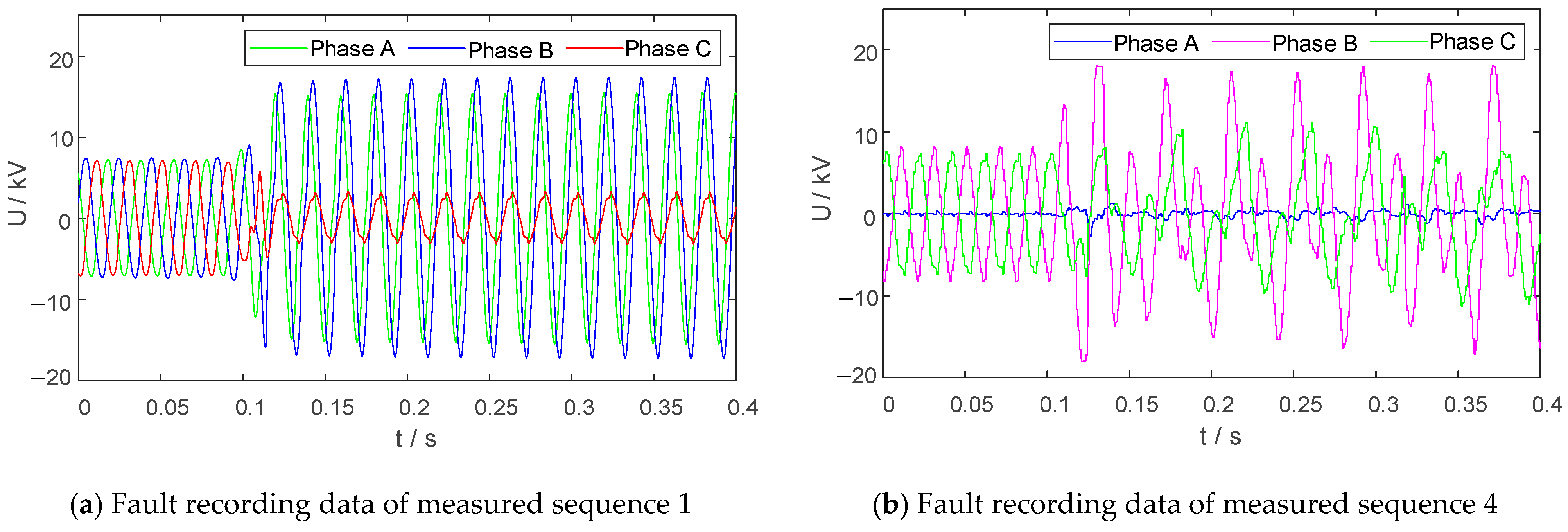
Measured data I were obtained from a 10 kV bus in an urban area of Yunnan Province. In this region, the earth capacitance $X_C$ and the excitation inductance $X_L$ of the PT fall within the resonance range (0.01 ≤ $X_C/X_L$ ≤ 0.5). When the system experiences disturbances such as single-phase grounding faults or no-load closing, ferroresonance may be triggered. In 2023, the 10 kV bus experienced over 20 ferroresonance incidents, which significantly impacted the power supply reliability in the region. To verify the accuracy of the proposed method under high-noise conditions, we selected three sets of fault recording data with high noise content for simulation validation (sequences 1 to 3, with a sampling frequency of 12.8 kHz and SNR approaching 20 dB). To further validate the effectiveness of the proposed method under low sampling rates, measured data II were obtained from fault recordings of another 10 kV bus in Yunnan Province, following the same sequence selection rules (sequences 4 to 6, with a sampling frequency of 5000 Hz). Partial fault recording data are shown in Figure 12.

For sequences 1 to 6 mentioned above, two power-frequency cycles are selected from each group for GASF encoding. Taking the data (a) and (b) in Figure 11 as an example, the encoded images are shown in Figure 13 and Figure 14.

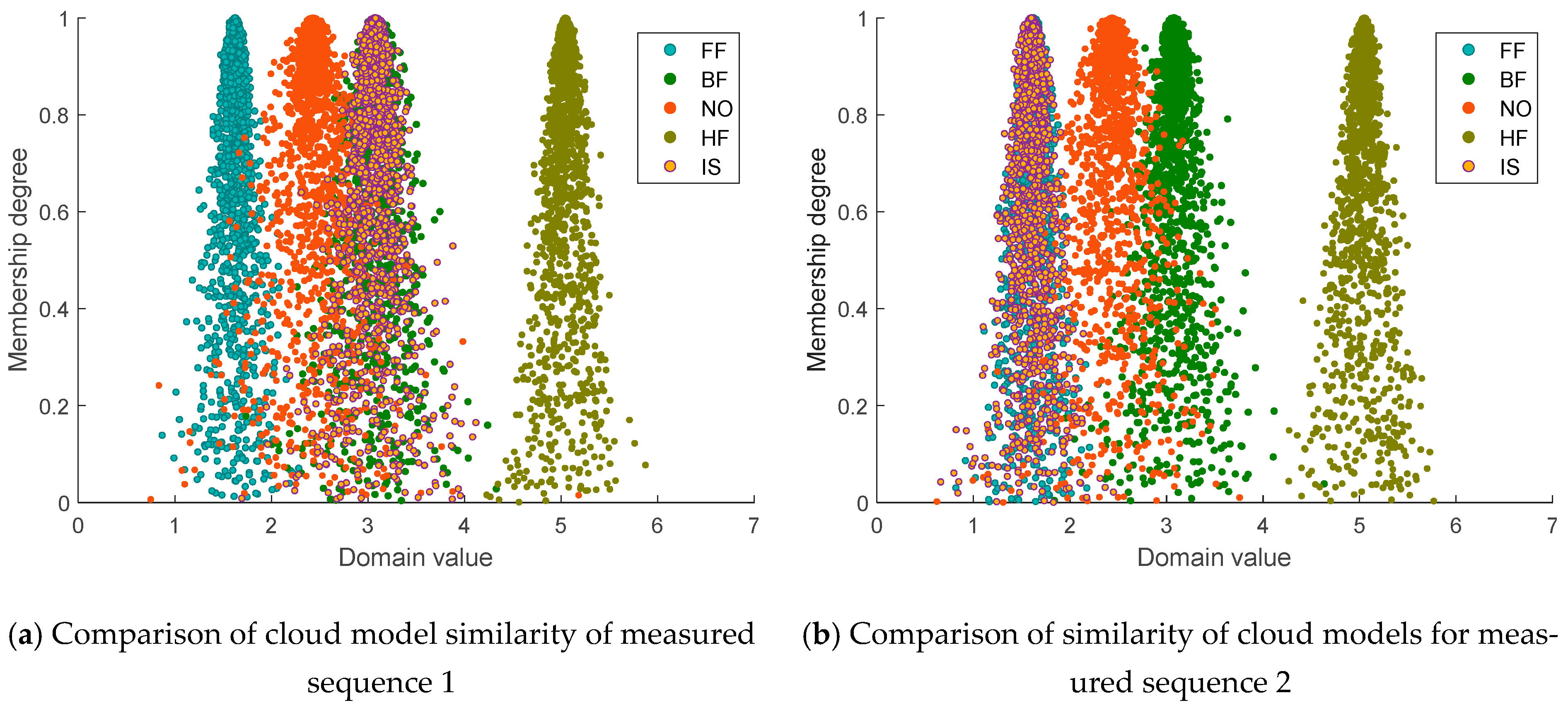
As shown in Figure 13 and Figure 14, the size of each phase point cluster in the measured fractional-frequency-resonance encoded image is significantly smaller than that of the standard-power-frequency signal, and the number of phase point centre clusters also decreases accordingly. The distribution of phase point clusters in the fundamental-frequency-resonance encoded image is similar to that of the power-frequency encoded image. However, the phase points within each cluster are randomly distributed and no longer symmetrical, and the depth of the grooves is unevenly distributed. This reconstructed image exhibits texture features consistent with those of the GASF-encoded images from the simulation part, indicating the feasibility of identifying resonance by extracting texture features from the reconstructed ferroresonance images. The texture features of the GASF images of the measured data sequences were extracted using GLCM, and the improved cloud model method was employed to identify the resonance type of the measured sequences. The similarity comparison of the cloud models of sequence 1 and sequence 4 is shown in Figure 15, where IS stands for identification signal.

As shown in Figure 15, the standard cloud models of measured sequences 1 and 2 coincide with the fundamental-frequency-resonance index cloud model and the fractional-frequency-resonance index cloud model, respectively. By calculating the membership degree between the standard cloud of the measured sequence and the index clouds of different resonance types using Equation (24), the specific resonance type can be determined when the membership degree meets the threshold requirement. For instance, for measured sequence 1, the membership degree between its standard cloud and the fundamental-frequency-resonance index cloud is ≥ 95%, indicating that this sequence corresponds to fundamental-frequency resonance. The identification results for all measured sequences are summarized in

Table 5. Results of measured data identification.

Sequence	VMD	Phase Space Reconstruction	Proposed Method
1	/	fundamental frequency	fundamental frequency
2	/	fundamental frequency	fundamental frequency
3	fractional frequency	/	fractional frequency
4	fractional frequency	/	fractional frequency
5	fractional frequency	/	fractional frequency
6	/	fundamental frequency	fundamental frequency

.

As shown in Table 5, the VMD method identifies resonance by extracting the frequency-domain features of the resonance signal. For resonance types such as sequences 3 to 5, which exhibit distinct frequency-domain characteristics, the VMD method achieves a 100% identification accuracy rate. However, for sequences 1 and 2, which are ferroresonances with oscillation frequencies at the power frequency, the VMD method loses its identification capability due to interference from the power-frequency signal.

The PSR method introduces the resonance overvoltage time series into a two-dimensional phase space. It extracts the geometric features and attribute characteristics of the phase space reconstruction attractor for resonant identification. Since this method does not account for noise, it fails to identify high-noise-content time series (such as sequences 3 to 5), resulting in an identification accuracy rate of 0%. This indicates that the proposed resonance criterion is no longer applicable under such conditions.

The proposed method performs denoising processing on all sequences to be identified, ensuring the uniqueness of the mapping relationship between the GASF image and the time series. Consequently, when dealing with high-noise-content sequences (such as sequences 3 to 5), the proposed method achieves a 100% identification accuracy rate. Additionally, by converting the overvoltage time series into GASF images for resonance identification, this method no longer relies on the frequency-domain features of the signal. Therefore, for fundamental-frequency resonances that VMD cannot effectively identify, this method also achieves an accuracy rate of 100%. In conclusion, the measured data demonstrate that the proposed method has high accuracy in resonance identification. Additionally, this method only requires extracting two resonance cycle voltage data points for resonance identification, eliminating the need for classifiers such as SVM or CNNs. This reduces the time required for dataset training and parameter adjustment, significantly shortening the fault discrimination time.

Based on the analysis and verification of the above measured data, it is evident that the algorithm proposed addresses existing issues in current ferroresonance identification methods, such as susceptibility to misjudgment, difficulty in setting thresholds, and low identification rates when extracting features from ferroresonance overvoltage signals. Furthermore, it is simple to operate and can complete resonance identification within two to three power-frequency cycles. Therefore, the proposed algorithm meets the requirements for rapidity and reliability in ferroresonance identification.

6. Conclusions

This paper addresses the challenges associated with traditional time-frequency analysis methods in extracting features from ferroresonance overvoltage signals, including misjudgment, threshold-setting difficulty, and sensitivity to noise interference. The SGMD algorithm is employed for denoising and reconstructing the overvoltage time series. Subsequently, the GASF method maps the reconstructed time series into two-dimensional images, from which texture features are extracted to facilitate accurate resonance identification. Through simulation analysis and case verification, the following conclusions are drawn:

(1)

The GASF image and the time series have a corresponding mapping relationship. Noise can obscure the evolution information of moving points. Therefore, this paper employs the SGMD algorithm to denoise the sequence to be identified, ensuring the uniqueness of the mapping relationship between the GASF image and the time series and avoiding misjudgment caused by noise.

(2)

GASF images can reveal the temporal correlation and modal differences among ferroresonance signals while preserving the numerical information in the time series. Consequently, this method enables precise characterization of the broad frequency-domain and nonlinear properties of ferroresonance overvoltage signals.

(3)

Ferroresonance exhibits self-sustaining characteristics. Consequently, the faster the identification rate, the less the system is affected by overvoltage. In the identification process, the method extracts only two power-frequency cycle data points for resonance identification without needing classifiers such as SVM or CNN, which reduces the time required for dataset training and parameter adjustment, significantly shortening the fault discrimination time.

(4)

Ferroresonance can induce overvoltage and overcurrent phenomena in power systems, posing a significant threat to the safe operation of electrical equipment. In extreme cases, it may result in equipment damage, malfunctioning of protective devices, and even large-scale blackouts and other critical incidents. Consequently, achieving accurate and rapid identification of ferroresonance is crucial for ensuring the safe and reliable operation of power systems.

The research objectives, identification method, and resonance criteria of this paper primarily focus on ferroresonance overvoltage. Given the similarities between ferroresonance overvoltage and arc grounding overvoltage in power systems, misjudgments may occur in practical applications. Therefore, future research will focus on analyzing the interference characteristics of various overvoltage signals in ferroresonance identification. By systematically collecting and quantifying the texture features of these signals, we will construct a multi-scale interference cloud model that integrates the noise coupling mechanism, aiming to enhance the universality and robustness of the proposed method in practical applications.