A Three-Channel Feature Fusion Approach Using Symmetric ResNet-BiLSTM Model for Bearing Fault Diagnosis

Abstract

For mechanical equipment to operate normally, rolling bearings—which are crucial parts of rotating machinery—need to have their faults diagnosed. This work introduces a bearing defect diagnosis technique that incorporates three-channel feature fusion and is based on enhanced Residual Networks and Bidirectional long- and short-term memory networks (ResNet-BiLSTM) model. The technique can effectively establish spatial-temporal relationships and better capture complex features in data by combining the powerful spatial feature extraction capability of ResNet and the bidirectional temporal modeling capability of BiLSTM. Specifically, the one-dimensional vibration signals are first transformed into two-dimensional images using the Continuous Wavelet Transform (CWT) and Markov Transition Field (MTF). The upgraded ResNet-BiLSTM network is then used to extract and combine the original one-dimensional vibration signal along with features from the two types of two-dimensional images. Finally, experimental validation is performed on two bearing datasets. The results show that compared with other state-of-the-art models, the computing cost is greatly reduced, with params and flops at 15.4 MB and 715.24 MB, respectively, and the running time of a single batch becomes 5.19 s. The fault diagnosis accuracy reaches 99.53% and 99.28% for the two datasets, respectively, successfully realizing the classification task.

1. Introduction

Rolling bearings work similarly to the train’s “ankle joints” and are crucial parts for the dependable operation of high-speed trains. They primarily serve to support loads, transmit alternating forces, and facilitate motion conversion [1]. Given the extensive operational hours and complex environmental conditions faced by high-speed trains in China, these bearings are frequently subjected to harsh environments characterized by elevated temperatures, severe shocks, and significant fluctuations in temperature and humidity. Consequently, monitoring their condition and implementing intelligent fault diagnosis for high-speed train bearings have become imperative for ensuring the safety and stability of train operations [2].

Numerous academic fields, including computer science, mechanics, mathematics, and signal processing, are involved in the study of rolling bearing defect identification. Scholars have been focusing more on machine learning and deep learning methods in recent years. These strategies use pattern recognition techniques and large data analysis to provide automated rolling bearing fault diagnosis [3]. Vibration signals from rolling bearings exhibit high sensitivity to early-stage faults and can effectively reflect changes in the condition of the bearing over time. Furthermore, advancements in vibration signal acquisition technologies have established them as one of the most widely utilized data sources for diagnosing faults in rolling bearings [4].

Time-domain analysis methods are capable of extracting comprehensive and complete information, enabling accurate analysis of the temporal characteristics of signals. These methods are particularly effective for analyzing non-periodic signals and demonstrate strong performance in fault diagnosis [5]. In order to diagnose faults, Zong et al. [6] used the Gini index in conjunction with three dimensionless time-domain features: average margin factor, average kurtosis factor, and average pulse factor. This information is fed into an Extreme Learning Machine (ELM) classifier to detect different defect kinds. Wang et al. [7] employed Singular Value Decomposition (SVD) to reconstruct the original signal, from which they extracted time-domain features along with power spectral entropy features that were successfully utilized in a classifier for fault classification purposes. Liang et al. [8] introduced one-dimensional time-domain signals into a one-dimensional extended convolutional network with residual connections to facilitate bearing fault diagnosis across various noise environments and loading conditions.

Single-feature defect diagnosis techniques are severely hampered by the non-stationarity of vibration signals from mechanical equipment. One interesting method for problem diagnostics has been identified as signal-to-image conversion [9]. Zhou et al. [10] presented a rolling bearing defect diagnosis technique that combines Vision Transformers (ViT), Convolutional Neural Networks (CNN), and Gramian Angular Field. The model’s fault diagnosis accuracies were 99.79% and 99.63%, respectively, following validation on two datasets. Hu et al. [11] applied the continuous wavelet transform to convert the bearing vibration signals into time-frequency images and then integrated these signals with the motor current data before feeding them into a network model. In various noise environments, the fault diagnosis accuracy reached 98%. These studies suggest that image-based signal transformation methods have great potential for application in rolling bearing fault diagnosis.

In bearing fault diagnosis, multi-channel data [12] can provide richer and more comprehensive fault information, effectively reducing the interference of random factors present in single-channel data. Sun et al. [13] embedded the representation patterns of rotating machinery faults from multi-modal information into an attention mechanism, focusing on extracting representative fault features with physical significance, thereby generating a universal representation of multi-modal information. Xu et al. [14] fused horizontal and vertical vibration signals using Principal Component Analysis (PCA), then employed Continuous Wavelet Transform to generate time-frequency feature maps, which were subsequently input into a residual neural network for feature extraction and classification. Using a model-data integrated digital twin system, Shi et al. [15] were the first to combine simulation signals with observed signals from rolling bearings displaying different fault modes. They then transformed 1D vibration signals into 2D images that contained time-frequency information using a Markov transition matrix-based image encoding technique. Using real bearing data, the created model’s effectiveness was evaluated. In order to create a multi-channel input network model that could simultaneously learn from these three image types, Gao et al. [16] used signal processing techniques to convert one-dimensional vibration signals into three different kinds of two-dimensional time-frequency images. The results show that the multi-channel technique achieved a 100% accuracy rate in fault diagnosis tasks compared to single-channel diagnostic models.

ResNet excelled in the field of deep learning, effectively extracting local and global features of vibration signals, and alleviating the problem of disappearing gradients through residual connections, making the training of deep networks more stable. Traditional machine learning methods, such as SVM and random forest, rely on artificial feature extraction and it is difficult to effectively capture complex time series dependencies. BiLSTM can capture the time series characteristics of the signal, taking into account both forward and backward information, thereby improving the ability to model time-dependent patterns. Combining spatial features extracted by ResNet with temporal features captured by BiLSTM can enhance the robustness and generalization ability of the model. With the advent of the big data era, the equipment monitoring data is growing exponentially, and the efficiency of single-mode signal processing methods is facing a challenge. At the same time, the computational burden of deep learning models has increased. Therefore, an enhanced ResNet-BiLSTM three-channel feature fusion method for bearing defect identification is proposed in this paper. The aim of this technique is to reduce the computational burden of deep models when processing multi-modal data while improving the effectiveness and accuracy of problem identification.

This paper’s remaining sections are arranged as follows. The fundamental ideas of the Continuous Wavelet Transform, Bidirectional Long Short-Term Memory Networks, Residual Neural Networks, Markov Transition Field, and Cross-Attention Mechanisms are presented in Section 2. The enhanced ResNet-BiLSTM three-channel feature fusion method’s construction is shown in Section 3. Two sets of bearing experimental data are used in Section 4 to examine the performance of the suggested approach. The conclusion and prospects are finally presented in Section 5.

2. Basic Theory

2.1. Continuous Wavelet Transform

The Continuous Wavelet Transform is a signal processing technique used for multi-scale analysis of signals, capturing their characteristics at different frequencies and time scales [17]. The basic principle is as follows:

The CWT decomposes and reconstructs the signal using a wavelet function. In order to efficiently capture the local aspects of the signal, a wavelet function is a localized function that can have localized properties in both the time and frequency domains. In order to acquire wavelet coefficients at several scales, the CWT convolves the signal with wavelet functions at distinct frequencies and scales. This allows for multi-scale analysis of the signal in both the frequency and temporal domains. The formula for CWT is given by Equation (1):

$$CW{T}_f\left(a,b\right)=\left[f\left(t\right),{\psi }_{a,b}\left(t\right)\right]={\displaystyle \frac{1}{\sqrt{a}}}{\displaystyle \int f\left(t\right)}{\psi }^{*}\left({\displaystyle \frac{t-b}{a}}\right)dt$$

(1)

Here, the mother wavelet is scaled and translated to produce A: ${\psi }_{a,b}\left(t\right)$

$${\psi }_{a,b}\left(t\right)={\displaystyle \frac{1}{\sqrt{a}}}\psi \left({\displaystyle \frac{t-b}{a}}\right)$$

(2)

In the equation, a is the scale factor, which corresponds to the scaling related to frequency, and b is the translation factor, $\psi$ represents the wavelet basis function.

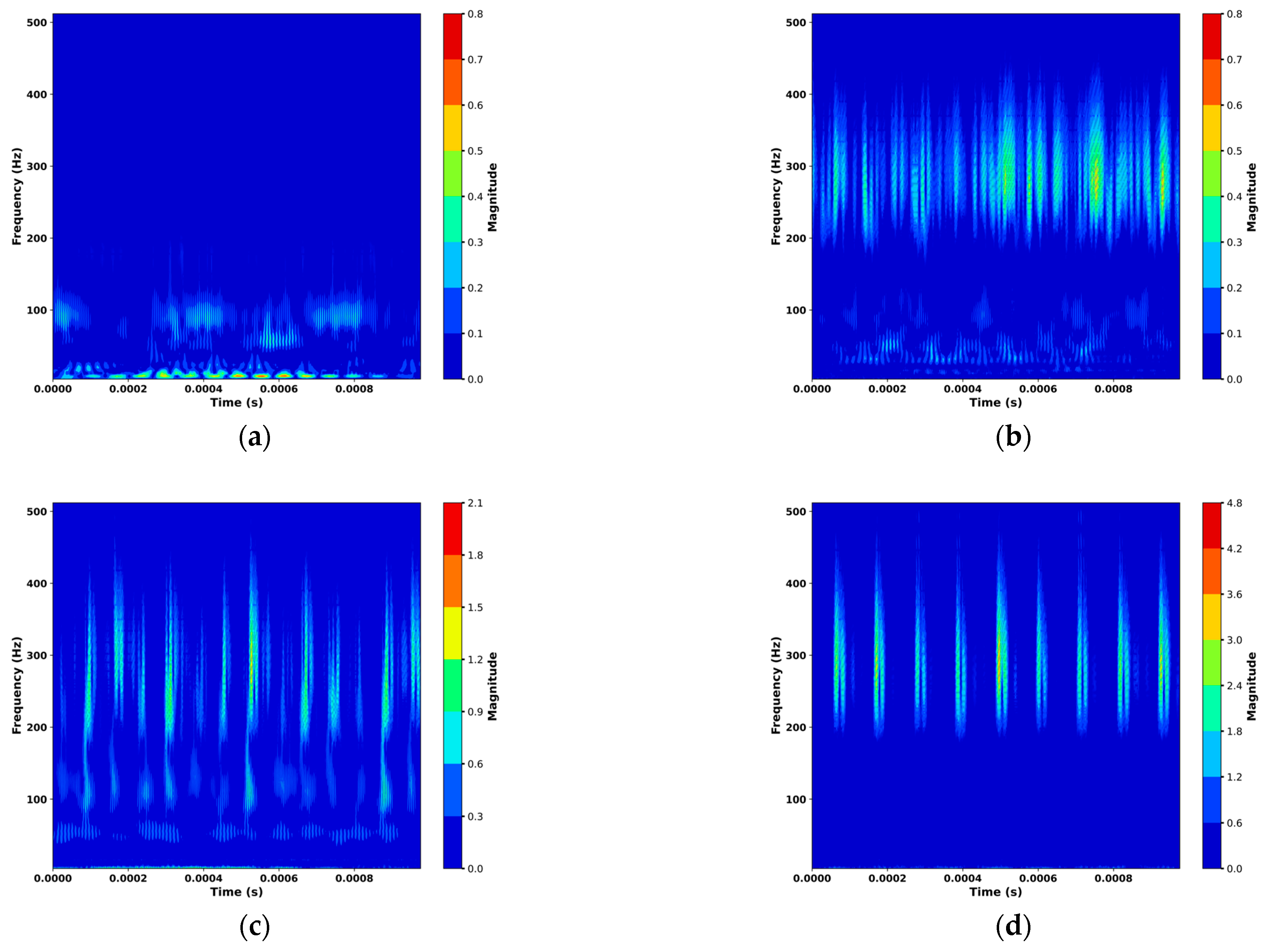
The Morlet wavelet is chosen as the wavelet basis function in this investigation because its waveform resembles the impact characteristics brought on by rolling bearing problems [18]. Figure 1a–d shows the CWT images of rolling bearings under four health states.

2.2. Markov Transition Field

The Markov Transition Field incorporates both temporal and spatial factors into the traditional Markov model, constructing a Markov transition matrix while preserving the temporal correlation of the original signal by transforming a one-dimensional time-domain signal into a two-dimensional image [19].

The original time-series signal X = {x₁, x₂ …, x_n} is divided into Q quantile regions based on the signal amplitude at different time instants. Each data point has distinct characteristics, and they are mapped to different quantile regions $q_i$ (i ∈ [1, Q]). hen, along the time axis, a Markov chain is used to calculate the transitions between quantile points, thereby constructing the Markov transition matrix D, as shown in Equation (3).

$$D=\left(\begin{array}{ccc}{d}_{11}& \dots & d_{1Q}\\ ⋮& \ddots & ⋮\\ d_{Q1}& \cdots & d_{QQ}\end{array}\right)=\left(\begin{array}{ccc}P\left(x_i\in q_1\left|x_{i-1}\in q_1\right.\right)& \dots & P\left(x_i\in q_1\left|x_{i-1}\in q_n\right.\right)\\ ⋮& \ddots & ⋮\\ P\left(x_i\in q_n\left|x_{i-1}\in q_1\right.\right)& \cdots & P\left(x_i\in q_n\left|x_{i-1}\in q_n\right.\right)\end{array}\right)$$

(3)

In the equation, $d_{ij}$ represents the probability of data points in the quantile region $q_i$ transitioning to the quantile region $q_j$. The dynamic probabilistic transitions within the time series data are not taken into account by the Markov state transition matrix, which solely computes the transition probabilities between successive time steps. Equation (4) illustrates how the Markov-Kernel Filter overcomes this constraint by producing a dynamic probability transition matrix M across time scales.

$$M=\left(\begin{array}{ccc}{M}_{11}& \dots & M_{1n}\\ ⋮& \ddots & ⋮\\ M_{n1}& \cdots & M_{nn}\end{array}\right)=\left(\begin{array}{ccc}{D}_{ij\left|x_i\in q_{i,}{x}_i\in q_i\right.}& \dots & D_{ij\left|x_i\in q_{i,}{x}_n\in q_i\right.}\\ ⋮& \ddots & ⋮\\ D_{ij\left|x_n\in q_{i,}{x}_i\in q_i\right.}& \cdots & D_{ij\left|x_n\in q_{i,}{x}_n\in q_i\right.}\end{array}\right)$$

(4)

Using the Markov probability transition matrix D, which is displayed in Equations (2) and (3), the MTF calculation steps entail calculating the transition probabilities between $x_1$ and $x_2$. For instance, $M_{12}$ stands for the transition probability from $x_1$ to $x_2$, or the likelihood of moving from the quantile unit, which contains $x_1$, to the quantile unit, which contains $x_2$. By consulting matrix D, the corresponding transition probability $d_{ij}$ is identified as the second element in the first row of the matrix, which is then used to construct the dynamic probability transition matrix MTF with dimension n × n. Figure 2a–d shows the MTF images of rolling bearings under four health states.

2.3. Residual Networks

Due to their remarkable feature extraction capabilities, residual networks—a common deep learning architecture—are employed extensively in a variety of domains, including image recognition and natural language processing [20]. This study employs two types of residual modules: the Bottleneck Block and the Identity Block. Additionally, the ScConv module is introduced in both blocks to replace the traditional 3 × 3 convolution layer, effectively reducing spatial and channel redundancies within the network.

2.3.1. Residual Block

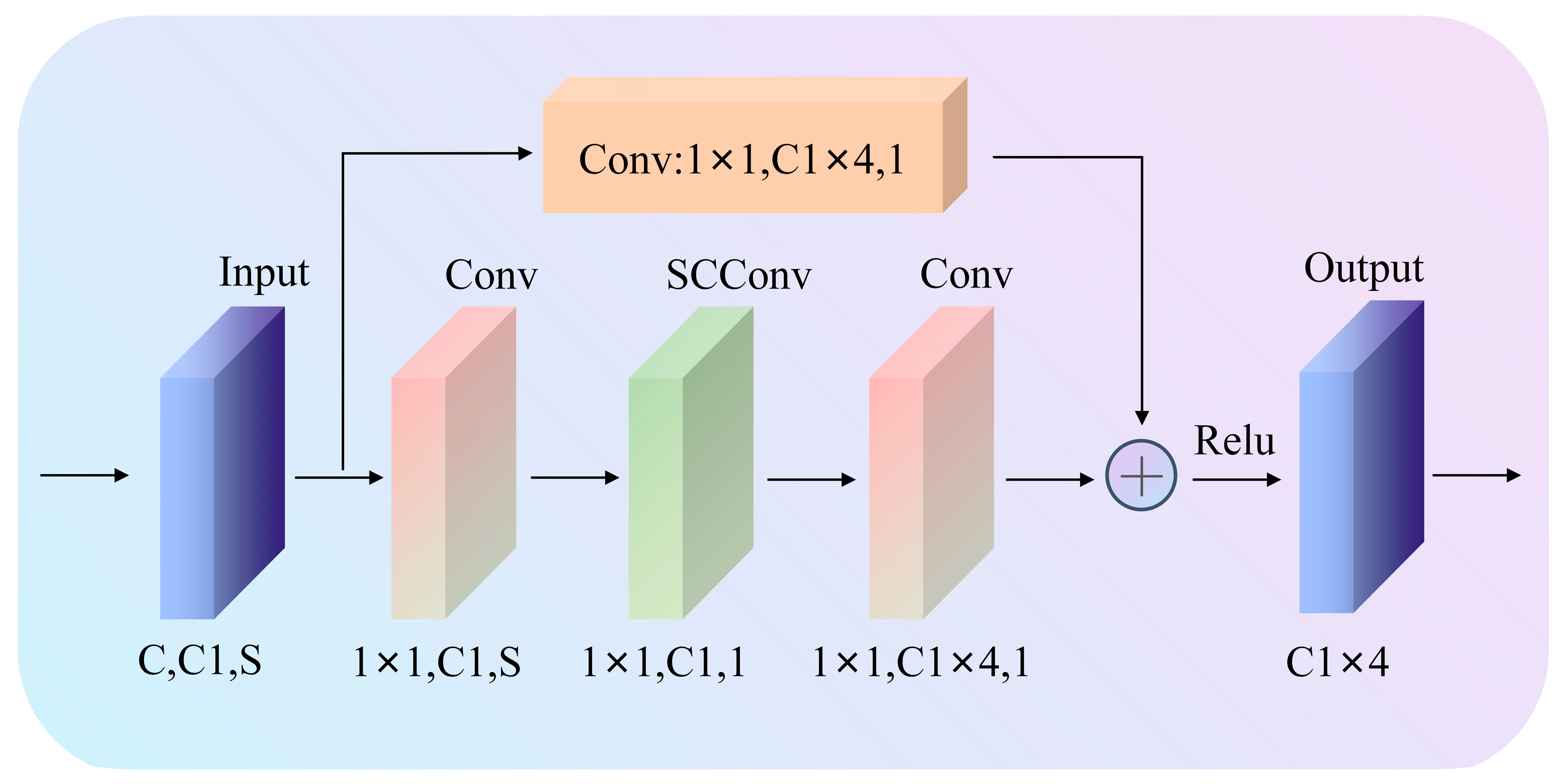
Figure 3 shows the Bottleneck Block’s convolutional structure. In order to lower the number of channels and, consequently, the number of parameters and computational complexity, this structure first employs a 1 × 1 convolution layer. After that, a ScConv module is used to extract features. Lastly, an up-scaling operation is performed using a second 1 × 1 convolution layer to restore the number of channels. This design’s benefit is that it can efficiently extract features while drastically cutting down on computation and parameters. It also helps with gradient backpropagation, which is particularly useful in networks with deeper structures. In the graphic, S stands for the convolution stride, C for the input channel number, and C1 for the output channel number.

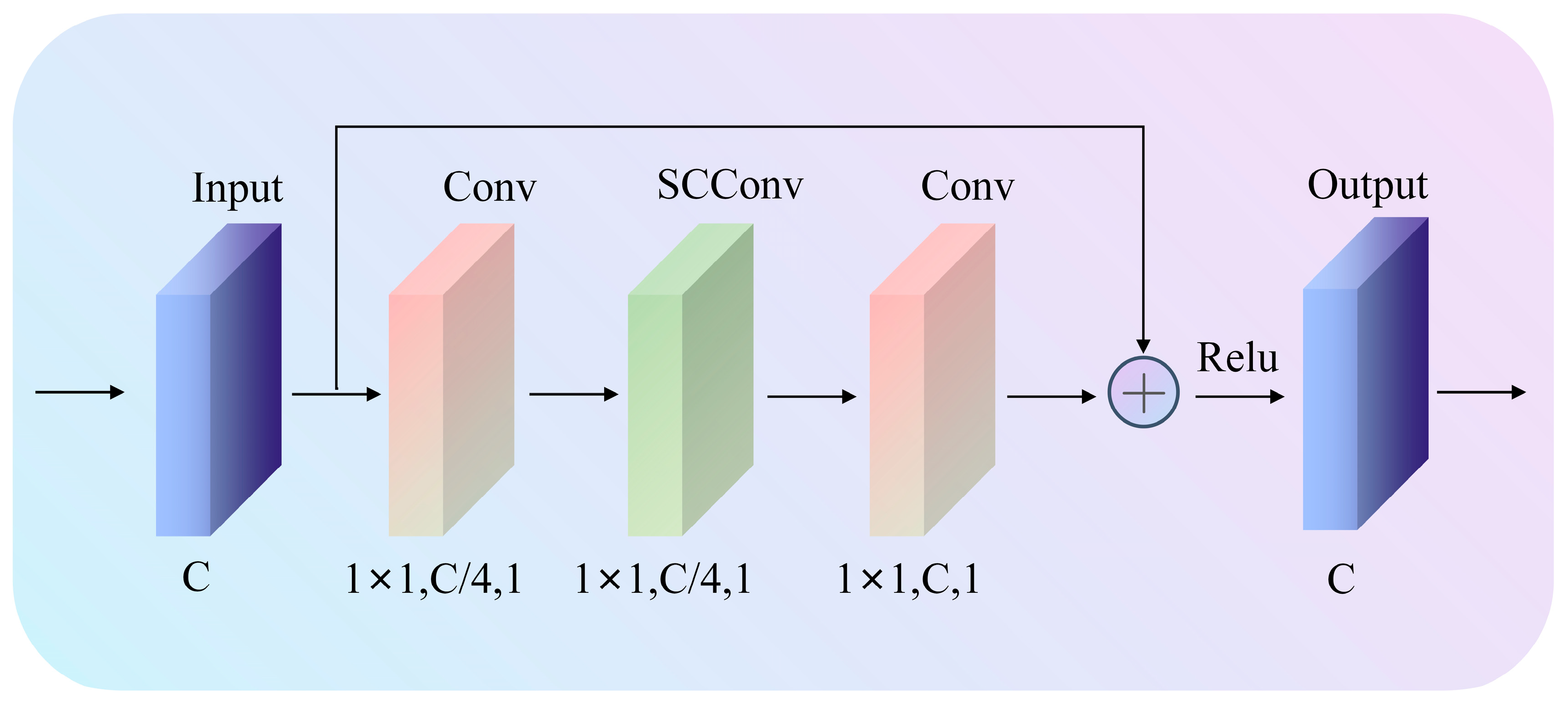
The Identity Block, shown in Figure 4, has a structure similar to the Bottleneck Block but with the same input and output dimensions, allowing them to be used in a sequential manner. The main purposes of this module are to deepen the network, solve the vanishing gradient issue, and successfully maintain the information’s integrity.

2.3.2. ScConv Module

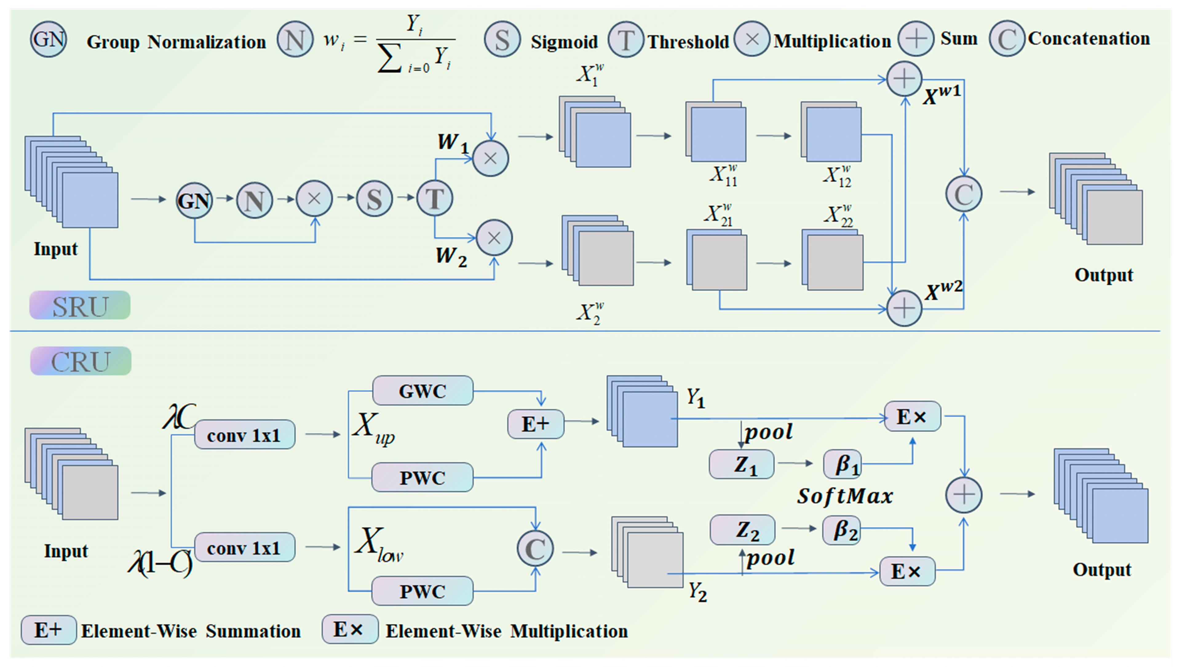
The ScConv module reduces both spatial and channel redundancy in convolutional neural networks by integrating the Spatial Reconstruction Unit (SRU) with the Channel Reconstruction Unit (CRU) [21]. Whereas the CRU maximizes channel features, the SRU maximizes spatial features. Lastly, the optimized features are transmitted to the subsequent convolutional block after being added to the initial residual connection. In Figure 5, the model structure is displayed.

The Spatial Reconstruction Unit (SRU) optimizes spatial features by separating and reconstructing the input feature X. Group normalization is applied as shown in Equation (5).

Equation (6) is used to produce the normalized weights, which indicate the relative relevance of various feature maps. A threshold is then utilized to apply gating after these weights are used to map the weighted features to the range (0, 1) using a Sigmoid function. By setting the threshold weight to 1 or 0.5, either full or partial information weights can be obtained with the specific calculation formula provided in Equation (7).

$$G{N}_{out}=GN(X)=\gamma {\displaystyle \frac{X-\mu }{\sqrt{{\sigma }^2+\epsilon }}}+\beta$$

(5)

$$W_{\gamma }=\{{\omega }_i\}={\displaystyle \frac{{\gamma }_i}{{\displaystyle {\sum }_{j=1}^C{\gamma }_i}}},i,j=1,2,\cdots ,C$$

(6)

$$W=Gate(sigmoid(W_{\gamma }(GN(X))))$$

(7)

In the equation, $\mu$ and $\sigma$ represents the mean and standard deviation, $\gamma$ and β are trainable variable and $\epsilon$ is a small constant used to ensure stability.

The reconstruction operation involves adding features with more information to those with less information, generating a more informative feature while saving space.

Equations (8) through (11) demonstrate how cross-reconstruction is used to merge two weighted features with disparate information to create $X^{\omega 1}$ and $X^{\omega 2}$, which are combined to produce the feature map with spatial refinement.

$$X_1^w=W_1\times X$$

(8)

$$X_2^w=W_2\times X$$

(9)

$$X_{11}^W+X_{22}^W=X^{w1}$$

(10)

$$X_{12}^W+X_{21}^W=X^{w2}$$

(11)

The Channel Reconstruction Unit (CRU) takes the spatially optimized features as input and generates channel-optimized features. CRU reduces channel redundancy through segmentation, transformation, and fusion operations while retaining the expressive power of the features.

The input spatially refined feature $X^{\omega }$ is split into two sections by the segmentation procedure, each with a channel size of λC and (1 − λ)C. Both feature sets are then compressed using convolutional kernels, producing $X_{up}$ and $X_{low}$.

The input is initially processed using pointwise convolution (PWC) and groupwise convolution (GWC) operations, which are carried out independently for each group. The output $Y_1$ is then obtained by adding the results. In order to generate the output $Y_2$, the input is further utilized as supplemental data and subjected to a pointwise convolution (PWC) [22].

The fusion operation utilizes a simplified SKNet method for the adaptive merging of $Y_1$ and $Y_2$ [23]. In particular, the pooled features $S_1$ and $S_2$ are obtained by first combining global geographical information and channel statistics using global average pooling. Then, a softmax function is applied to $S_1$ and $S_2$ to obtain the feature weight vector ${\beta }_1$ and ${\beta }_2$. Lastly, as indicated by Equation (12), the output Y is calculated using the feature weight vectors.

$$Y={\beta }_1{Y}_1+{\beta }_2{Y}_2$$

(12)

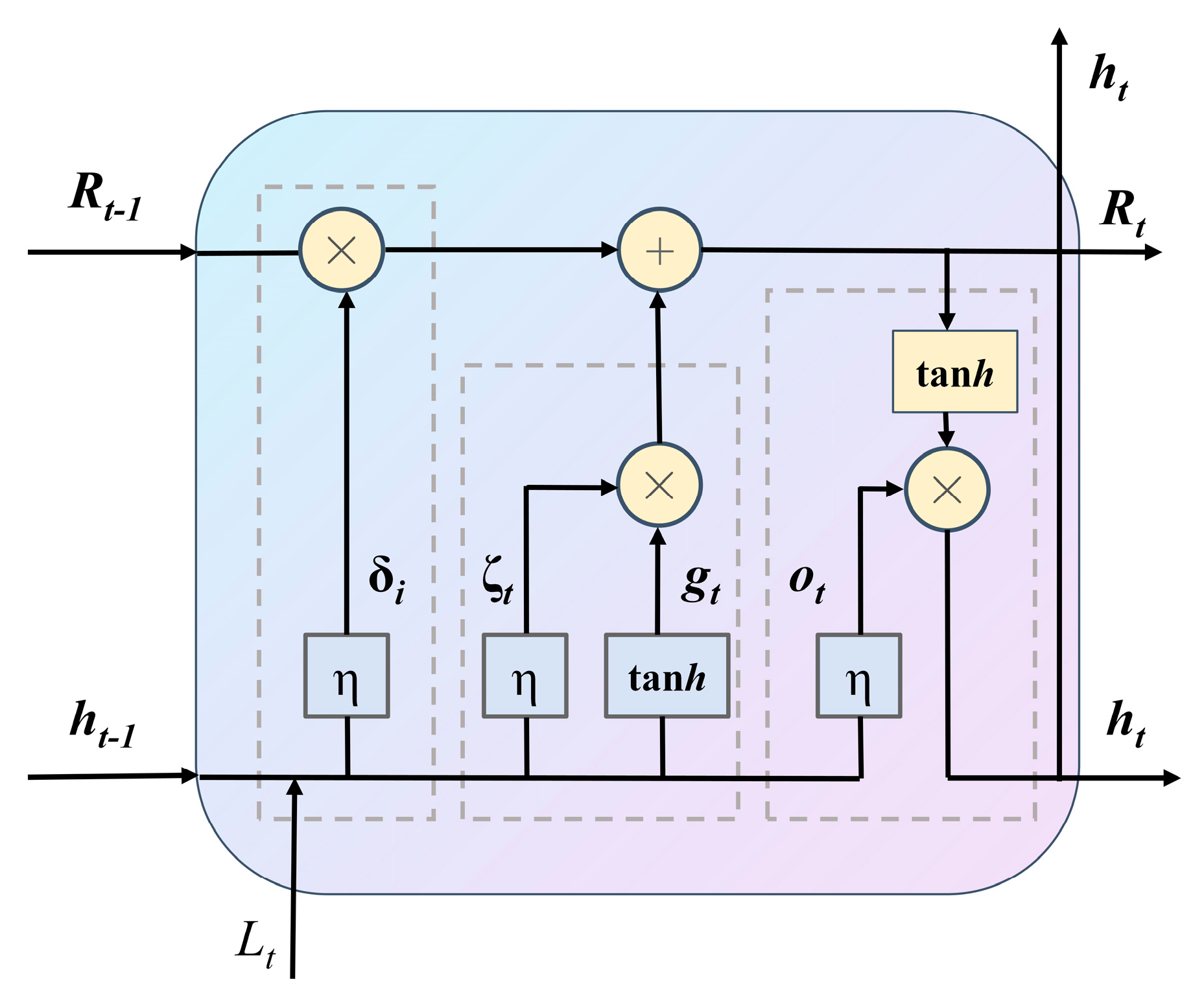
2.4. Bidirectional Long-And Short-Term Memory Networks

LSTM [24] effectively retains long-term dependent information by introducing memory units and gate mechanisms (forgetting gates, input gates, and output gates), mitigates the phenomenon of gradient vanishing, and provides a better fit for nonlinear prediction. The structure is shown in Figure 6. BILSTM processes the input sequences in 2 directions, forward and reverse, by means of 2 independent LSTM layers, respectively.

The Oblivion Gate is responsible for controlling the transfer of information and is mainly responsible for extracting some valid information from the external input:

$${\delta }_t=\eta (E_{\delta }[h_{t-1},L_t]+R_{\delta })$$

(13)

where ${\mathsf{\delta }}_t$ represents the forgetting gate’s input, η the activation function, ${\mathrm{E}}_s$ the forgetting gate’s input weight, $h_{t-1}$ the output state value at the previous instant, L_t the input amount, and R_s the forgetting gate’s deviation.

Whether or not fresh data is added to memory is determined by the input part of the gate:

$${\zeta }_t=\eta (E_{\zeta }[h_{t-1},L_t]+R_{\zeta })$$

(14)

$$g_t=\tanh (E_z[h_{t-1},L_t]+R_z)$$

(15)

where: ${\mathsf{\zeta }}_t$ is the input to the input gate; ${\mathrm{E}}_{\mathsf{\zeta }}$ is the input gate weight; ${\mathrm{R}}_{\mathsf{\zeta }}$ is the input gate deviation; $g_t$ is the candidate unit state; ${\mathrm{E}}_{\mathrm{z}}$ is the memory unit weight; and ${\mathrm{R}}_{\mathrm{z}}$ is the memory unit deviation.

Where the candidate unit state is denoted by ${\mathrm{g}}_{\mathrm{t}}$, the memory unit weight by ${\mathrm{E}}_{\mathrm{z}}$, the input gate weight by ${\mathrm{E}}_{\mathsf{\zeta }}$, the input gate deviation by ${\mathrm{R}}_{\mathsf{\zeta }}$, the input gate input by ${\mathsf{\zeta }}_t$, and the memory unit weight by ${\mathrm{R}}_{\mathrm{z}}$.

The output gate is responsible for deciding the output.

$$o_t=\eta (E_o[h_{t-1},L_t]+R_o)$$

(16)

$$o_t=f(\overrightarrow{E_h}\overrightarrow{h_t}+\overrightarrow{E_h}\overrightarrow{h_{t-1}}+R_t)$$

(17)

where: $o_t$ is the input to the input gate; E_t is the output gate weight; R_t is the output gate deviation; $\stackrel{⃑}{E_h}$ and $\overleftarrow{E_h}$ re the forward and backward connection weights; $\stackrel{⃑}{h_t}$ and $\overleftarrow{h_{t-1}}$ are the forward and backward output state values; and ${\mathrm{R}}_{\mathrm{t}}$ is the output gate deviation.

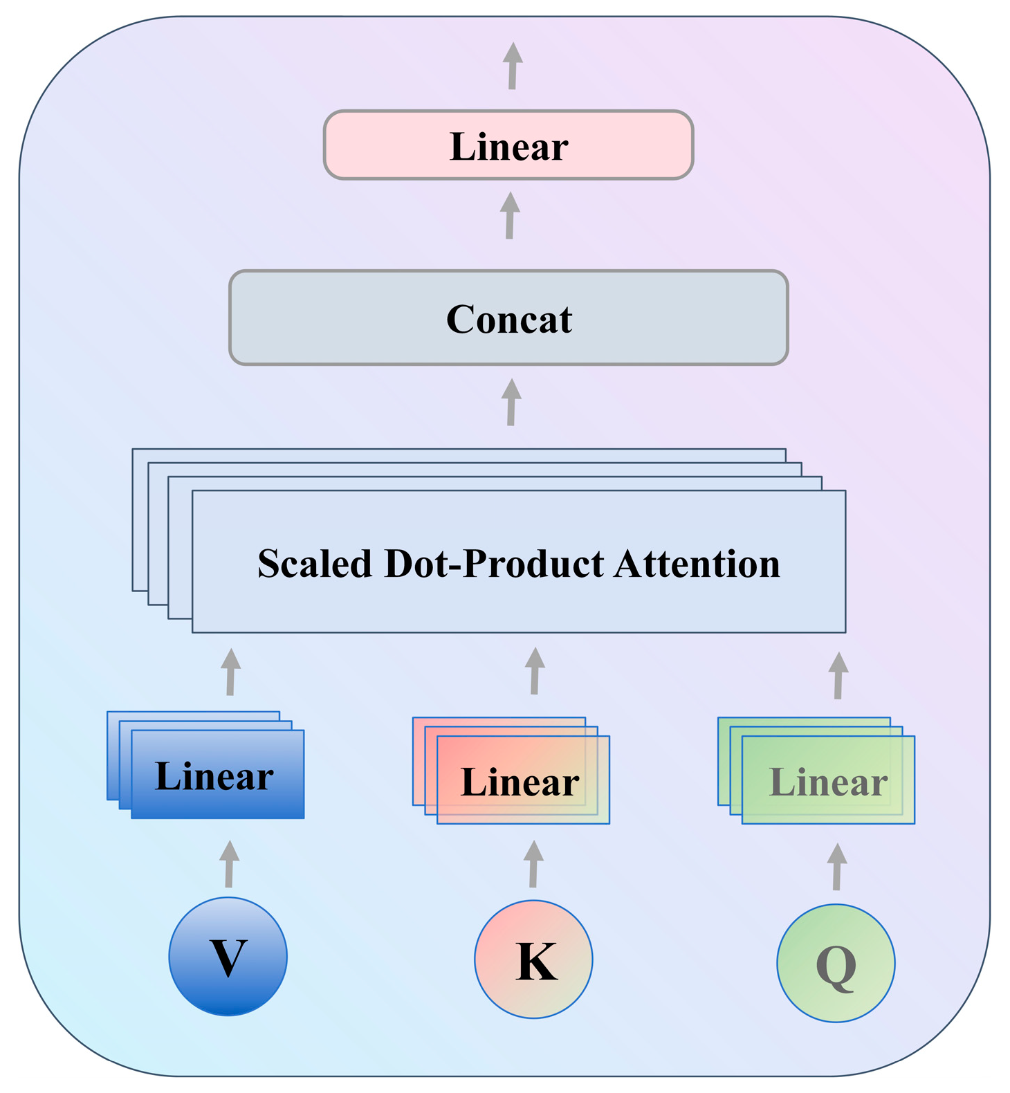
2.5. Cross-Attention Mechanism

The cross-attention mechanism’s computation method is comparable to that of the self-attention mechanism and is based on the calculation of Query, Key, and Value: A self-attention mechanism’s queries, keys, and values originate from a single input sequence, whereas a cross-attention mechanism’s queries originate from one input sequence and its keys and values from another, the structure is shown in the Figure 7 [25].

The computational steps are as follows:

First, the input query, key and value are transformed using a linear layer.

The query Q is dot-producted with the key K to determine the correlation score between the two inputs. Using the linear layer, the correlation score between the two inputs is determined. Here is the formula.

$$OU{T}_{attention}=soft\max ({\displaystyle \frac{Q{K}^T}{\sqrt{d_k}}})$$

(18)

where, ${QK}^T$ is the dot product of the query and the keys, which represents the similarity of the two sequences at different positions, and $d_k$ is the dimension of the keys, which is used as a scaling factor to avoid too large values.

Calculate the attention weights: convert these similarities into probability distributions by means of the softmax function, which represents the attention weights of the query for each key.

Weighted summation: these attention weights are applied to the values V to end up with the output vector. This is equivalent to extracting the attention information from the sequence of values and feeding it into the next network layer.

3. Three-Channel Feature Fusion Model Based on Improved Resnet-BiLSTM

In order to solve the problem of bearing defect diagnostics under different load scenarios, this study proposes a unique three-channel feature fusion technique based on the integration of bidirectional long and short-term memory networks and an improved residual neural network. First, the Markov variation field and continuous wavelet transform are used to convert the one-dimensional data into picture form. The 2D-ResNet-BiLSTM structure is then used to extract features from the two types of images independently, which are then supplied into the cross-attention mechanism by weighted fusion. Simultaneously, the fully connected layer classifies the one-dimensional signals that have been retrieved from the 1D-ResNet-BiLSTM structure and paired with the 2D features to feed into the cross-attention mechanism. Figure 8 depicts the general model structure of the suggested approach.

The one-dimensional data has an initial shape of 32 × 1024, which is extended to a dimension of 32 × 1 × 1024 by the unsqueeze (1) operation in PyTorch and input into the 1D-Resnet-BiLSTM structure after continuous wavelet and Markov variation field processing, the data is converted into a two-dimensional image with a shape of 32 × 224 × 224 × 3 and input into the 2D-Resnet-BiLSTM structure. Each Resnet module contains a Bottleneck Block and an Identity Block, arranged in the order shown in Figure 8; the specific output of each feature extraction module is shown in

Table 1. Feature Extraction Module Output Shape.

Network Module	Output Size	Network Module	Output Size
1D_Conv1	32 × 16 × 1024	2D_Conv1	32 × 112 × 112 × 64
1D_Pool	32 × 16 × 512	2D_Pool	32 × 56 × 56 × 64
1D_Resnet	32 × 16 × 512	2D_Resnet_1	32 × 28 × 28 × 256
1D_Conv2	32 × 1 × 512	2D_Resnet_2	32 × 14 × 14 × 512
1D_BILSTM	32 × 49 × 512	2D_Resnet_3	32 × 7 × 7 × 1024
		2D_BILSTM	32 × 49 × 512

.

The features processed by continuous wavelet transform and Markov variation field are weighted and fused and input into the cross-attention mechanism, which is calculated as shown in Equation (19):

$$featur{e}_{2d}={\vartheta }_{1}C+{\vartheta }_{2}M$$

(19)

where ϑ₁ = ϑ₂ = 0.5, C is the feature extracted by the continuous wavelet image transform channel, and M is the feature extracted by the Markov transform field image transform channel.

4. Experimentation and Analysis

A bearing life prediction test bed, a PC with an i5-7300HQ processor, and an RTX 1050 graphics card are among the tools used for the studies in this study. The PyTorch (v2.3.0) deep learning framework was used for model training and experimental validation.

Western Reserve University’s bearing data and the experimental data obtained from the bearing life prediction test bed were used to validate the trials.

4.1. Indicators for Model Evaluation

This work employs four assessment metrics—Precision, Recall, F1 Score, and Accuracy—to assess the effectiveness of the proposed method and to compare it with leading contemporary methods.

$$Precision={\displaystyle \frac{TP}{TP+FP}}$$

(20)

$$Recall={\displaystyle \frac{TP}{TP+FN}}$$

(21)

$$\begin{array}{cc}{F}_1& Score\end{array}={\displaystyle \frac{2*(Precision*Recall)}{Precision+Recall}}$$

(22)

$$Accuracy={\displaystyle \frac{TP+TN}{TP+TN+FP+FN}}$$

(23)

where TP denotes true positive, TN denotes true negative, FP denotes false positive, and FN denotes false negative.

4.2. CWRU Dataset Validation

4.2.1. Sample Division of the Dataset

Bearing sampling parameters are set as follows: sampling frequency is 12 kHz, motor speed is 1772 rpm, and bearing load is 1 HP. For every load, the bearings were in one of four health states: roller failure, inner ring failure, outer ring failure, or normal state. As shown in

Table 2. CWRU data classification.

Damage Type	Damage Size	Sample Count	Tag
Normal	None	233	0
Inner	0.007 inch	233	1
	0.014 inch	233	2
	0.021 inch	233	3
Ball	0.007 inch	233	4
	0.014 inch	233	5
	0.021 inch	233	6
Outer	0.007 inch	233	7
	0.014 inch	233	8
	0.021 inch	233	9

, each failure condition has three distinct damage levels: 0.007 inches, 0.014 inches, and 0.021 inches, in addition to the healthy state. The length of each sample data point is 1024, and the overlap rate is 0.5. After perturbation with random seeds, all 2330 samples were finally created and divided into training, validation, and test sets in the ratio of 60%:20%:20%.

4.2.2. Ablation Experiments

This work designs six sets of ablation experiments to compare with the suggested method in order to confirm the significance of each component in the proposed model. Each group of ablation experiments is described in

Table 3. Model description and accuracy.

Model	Description
Model-1	1D_Sc-Resnet + BILSTM
Model-2	CWT + MKF + 2D_Sc-Resnet + BILSTM + Attention
Model-3	CWT + MKF + 1D&2D_Sc-Resnet + Attention
Model-4	CWT + 1D&2D_Sc-Resnet + BILSTM + Attention
Model-5	MKF + 1D&2D_Sc-Resnet + BILSTM + Attention
Model-6	CWT + MKF + 1D&2D_Sc-Resnet + BILSTM
Model-7	CWT + MKF + 1D&2D_ Resnet + BILSTM + Attention
Proposed Model	CWT + MKF + 1D&2D_Sc-Resnet + BILSTM + Attention

. Model-1 only contains the one-dimensional data feature extraction module of the proposed Model. Model-2 includes a 2-D data feature extraction module of the proposed Model. Compared with the proposed Model, Model-3 lacks a BILSTM structure. Model-4 includes a one-dimensional data feature extraction module and a wavelet transform two-dimensional data feature extraction module. Model-5 includes a one-dimensional data feature extraction module and Markov transform two-dimensional data feature extraction module. Model-6 lacks Attention structure; Model-7 lacks ScConv structure and uses residual blocks of normal structure, and

Table 4. Evaluation indexes of each model in ablation experiment.

Model	Params	Flops	Batch	Precision (Avg)	Recall (Avg)	F1 Score (Avg)	Accuracy (Avg)
Model-1	4.49 MB	318.53 MB	2.41 s	87.35% ± 0.15%	87.04% ± 0.13%	87.19% ± 0.16%	87.04% ± 0.14%
Model-2	15.11 MB	681.77 MB	4.35 s	96.69% ± 0.12%	96.25% ± 0.14%	96.47% ± 0.13%	96.24% ± 0.14%
Model-3	11.2 MB	544.17 MB	4.17 s	96.63% ± 0.14%	96.64% ± 0.16%	96.63% ± 0.15%	96.64% ± 0.17%
Model-4	8.4 MB	420.13 MB	3.09 s	98.36% ± 0.12%	98.31% ± 0.10%	98.33% ± 0.13%	98.32% ± 0.15%
Model-5	8.4 MB	420.13 MB	3.09 s	98.32% ± 0.13%	98.28% ± 0.15%	98.29% ± 0.12%	98.28% ± 0.12%
Model-6	14.32 MB	659.71 MB	4.74 s	97.54% ± 0.11%	97.67% ± 0.10%	97.41% ± 0.14%	97.54% ± 0.13%
Model-7	24.37 MB	1.28 G	12.05 s	99.36% ± 0.10%	99.31% ± 0.12%	99.33% ± 0.09%	99.31% ± 0.11%
Proposed Model	15.4 MB	715.24 MB	5.19 s	99.56% ± 0.08%	99.55% ± 0.10%	99.56% ± 0.09%	99.53% ± 0.08%

shows the mean and standard deviation of precision, recall, F1 score, and accuracy as well as params, flops, and individual batch run time for each group of models on the test set, repeated experiments were validated using K-fold cross-validation, with a value of 5 selected for K while Figure 9a–h displays the confusion matrix.

Through the setup of ablation experiments, it is shown that the combination of features of different dimensions can successfully realize the complementary information and provide a rich basis for analysis and decision-making; the addition of BiLSTM and Attention can effectively mine the bidirectional spatio-temporal features and enhance the feature expression ability; moreover, the addition of Ssconv reduces the number of params and flops, and dramatically improves the computational efficiency. Therefore, the proposed model has an efficient and accurate design as well as excellent performance.

4.2.3. T-SNE Visualization

To confirm how the number of 2D-Resnet layers affects the model’s performance, we additionally employ the t-SNE visualization technique. As illustrated in Figure 10, the classification effect of the test set samples is visualized using one 2D-Resnet, two 2D-Resnets, and three 2D-Resnets, respectively.

The samples of different categories in (a) overlap seriously and the sample points of the same category are widely spaced, which indicates that the classification effect of one 2D-Resnet is not good; (b) the sample classification effect of each category is improved obviously, but there are still some intersections between some categories; (c) the sample classification effect of each category is optimal; therefore, the network model with three 2D-Resnet layers is able to achieve optimal sample classification.

4.2.4. Comparison with Advanced Models

In order to prove the superiority of the proposed model, this paper also compares it with four state-of-the-art models; DCNN-WOA-DELM [26] sends the one-dimensional data features extracted by DCNN to the WOA-DELM model for bearing fault diagnosis. MCR-KA-Resnet [27] model fuses the three transformed images of MTF, CWT, and RP and uses the improved residual network for feature extraction and classification. IG-CWT-VGG [28] model first performs gradient optimization on one-dimensional data and then transforms it into a CWT image for feature extraction and classification using the VGG model. The MTF-MARN [29] model converts one-dimensional vibration signals into two-dimensional MTF images as input to the residual network and adds mixed attention mechanism to the residual structure to enhance the feature extraction capability; each model uses the Western Reserve University public bearing dataset, repeated experiments were validated using K-fold cross-validation, with a value of 5 selected for K.

Table 5. Evaluation indicators compared with advanced models.

Model	Params	Flops	Batch	Precision (Avg)	Recall (Avg)	F1 Score (Avg)	Accuracy (Avg)
DCNN-WOA-DELM	32.33 M	1.81 G	10.2 s	99.33% ± 0.15%	99.29% ± 0.18%	99.31% ± 0.17%	99.32% ± 0.16%
MCR-KA-Resnet	27.2 M	2.52 G	8.23 s	99.40% ± 0.12%	99.35% ± 0.14%	99.35% ± 0.13%	99.36% ± 0.14%
IG-CWT-VGG	78.4 M	8.41 G	12.25 s	99.52% ± 0.14%	99.52% ± 0.16%	99.48% ± 0.15%	99.51% ± 0.17%
MTF-MARN	34.2 M	2.30 G	9.15 s	99.50% ± 0.12%	99.48% ± 0.10%	99.51% ± 0.13%	99.48% ± 0.15%
Proposed Model	15.4 MB	715.24 MB	5.19 s	99.56% ± 0.08%	99.55% ± 0.10%	99.56% ± 0.09%	99.53% ± 0.08%

contains the average and standard deviation of Precision, Recall, F1 Score, and Accuracy, along with Params, Flops, and individual batch run time.

In addition, the confusion matrix of the four advanced models is shown in Figure 11a–d, and the confusion matrix of the proposed model is shown in Figure 9h.

Experimental results show that the proposed model achieves excellent performance on all evaluation metrics. Feature fusion allows the model to perform more consistently under different data characteristics or signal quality, avoiding performance fluctuations that may result from a single feature dimension. The excellent performance of the proposed model highlights its effectiveness in solving classification tasks, with particularly significant improvements in recall and F1 scores, and these results demonstrate the effectiveness of the proposed approach in achieving fault classification.

4.3. Validation of Simulated Condition Data Set

4.3.1. Lab Bench Description and Sample Division

The bearing life prediction test bench is used to simulate the fault bearing condition of high-speed trains under normal operating conditions. A vibration acceleration sensor and data acquisition device were used to collect bearing vibration data under various fault conditions. Hydraulic cylinder, oil pump, gear pump, operating platform, oil tank, data collector and other equipment constitute most of the unique components of the experimental device, as shown in Figure 12.

A frequency of 20 kHz, a sampling length of 6 s, a motor speed of 1000 rpm, and bearing loads of 0 N, 1000 N, and 2000 N are used to sample the vibration data of the bearings used for the experiments in this section. There are four different health states for the bearings under each load, as indicated in

Table 6. Bearing life prediction test bench data classification.

Damage Type	Load	Sample Count	Tag
Normal	0	233	0
	1000	233	1
	2000	233	2
Inner	0	233	3
	1000	233	4
	2000	233	5
Ball	0	233	6
	1000	233	7
	2000	233	8
Outer	0	233	9
	1000	233	10
	2000	233	11

.

For every sample, there are 1024 data points, and the overlap rate is 0.5. After perturbation with random seeds, all 2796 samples were finally created and divided into training, validation, and test sets in the ratio of 60%:20%:20%.

4.3.2. Experimental Result

This research compares the suggested model with the conventional model LSTM and the combined model of VGG16 [30], Resnet34, and Swin Transformer [31] in order to demonstrate its superiority. The application of LSTM on one-dimensional time series efficiently handles the prediction, classification, and generation tasks of sequence data by capturing long-term dependencies and temporal features; VGG16 realizes efficient classification performance by deep convolutional network to extract hierarchical image features and achieve efficient classification performance; ResNet34 solves the problem of gradient vanishing in deep network training by introducing residual structure, thus improving classification accuracy and model stability; Swin Transformer achieves efficient fusion and classification of global and local information of images through local attention mechanism and multi-scale feature extraction; each of the models all use the bearing dataset measured by the bearing experimental bench, repeated experiments were validated using K-fold cross validation, with a value of 5 selected for K.

Table 7. The evaluation index is compared with the traditional model.

Model	Params	Flops	Batch	Precision (Avg)	Recall (Avg)	F1 Score (Avg)	Accuracy (Avg)
LSTM + VGG16	142.2 M	15.54 G	18.20 s	96.36% ± 0.23%	96.20% ± 0.21%	96.27% ± 0.19%	96.29% ± 0.22%
LSTM + Resnet34	26 M	3.64 G	15.40 s	97.88% ± 0.18%	97.63% ± 0.15%	97.75% ± 0.17%	97.63% ± 0.16%
LSTM + Swin Transformer	32.2 M	4.54 G	10.25 s	97.08% ± 0.20%	97.05% ± 0.18%	97.10% ± 0.16%	97.07% ± 0.19%
Proposed Model	15.4 MB	715.24 MB	5.19 s	99.30% ± 0.07%	99.27% ± 0.08%	99.29% ± 0.06%	99.28% ± 0.07%

contains the average and standard deviation of precision, recall, F1 Score, and accuracy, along with params, flops, and individual batch run time.

Additionally, the classification performance test results of the suggested approach with the other three methods for the test set samples are visualized using the confusion matrix in Figure 13.

The experimental results show that although the combined model can realize the classification of different categories of fault features, there still exists a small amount of sample confusion between individual categories, while the proposed model, through the improved residual structure with the invocation of the attention mechanism, shows a significant improvement in the precision, recall, F1 score, and accuracy. Therefore, the proposed model has obvious advantages in the field of fault diagnosis.

5. Conclusions and Discussion

The following is a summary of the key findings of this paper’s suggested three-channel feature fusion fault diagnostic approach, which is based on an enhanced ResNet-BiLSTM model:

• Continuous wavelet transform and Markov variation field are used to transform one-dimensional vibration signals into two-dimensional images. This helps to understand the dynamic changes in time series by revealing the possible relationship between time and frequency and illustrating the probability of system state transfer.
• The one-dimensional time series features and two-dimensional image features are fused using a cross-attention mechanism that can capture the intricate dependencies between various modes and dynamically adjust the information flow between the features, further improving the model’s generalization ability. The two-dimensional image features are processed using a weighted fusion strategy, which increases the complementarity of the features and decreases the redundant information.
• The model achieves 99.53% and 99.28% recognition accuracy on the public bearing dataset and the simulated real-world working condition dataset, respectively, demonstrating its outstanding classification performance across various bearing datasets.

Despite the exceptional performance of the approach shown in this study, real-time performance, data reliance, and computational complexity can all be improved. Future studies can concentrate on improving the model’s interpretability, maximizing its computational efficiency, and determining how to further boost the model’s performance in situations involving real-time applications and small data volumes.

References

1. Mohammed, H.K.; Ali, N.A. A systematic review of rolling bearing fault diagnoses based on deep learning and transfer learning: Taxonomy, overview, application, open challenges, weaknesses and recommendations. Ain Shams Eng. J. 2023, 14, 101945. [Google Scholar] [CrossRef]
2. Wang, C.P.; Qi, H.Y.; Hou, D.M. Ensefgram: An optimal demodulation band selection method for the early fault diagnosis of high-speed train bearings. Mech. Syst. Signal Process. 2024, 213, 111346. [Google Scholar] [CrossRef]
3. Govind, V.; Sumika, C.; Mert, S. A roadmap to fault diagnosis of industrial machines via machine learning: A brief review. Measurement 2025, 242, 116216. [Google Scholar] [CrossRef]
4. Omri, M.; Itai, D.; Jacob, B. A systematic literature review of deep learning for vibration-based fault diagnosis of critical rotating machinery: Limitations and challenges. J. Sound Vib. 2024, 590, 118562. [Google Scholar] [CrossRef]
5. Riku, N.; Konsta, K.; Mika, P. Automation of low-speed bearing fault diagnosis based on autocorrelation of time domain features. Mech. Syst. Signal Process. 2020, 138, 106572. [Google Scholar] [CrossRef]
6. Zong, M.; Ying, Z.; Bo, Z. Research on rolling bearing fault diagnosis method based on ARMA and optimized MOMEDA. Measurement 2022, 189, 110465. [Google Scholar] [CrossRef]
7. Wang, S.Q.; Lian, G.G.; Cheng, C. A novel method of rolling bearings fault diagnosis based on singular spectrum decomposition and optimized stochastic configuration network. Neurocomputing 2024, 574, 127278. [Google Scholar] [CrossRef]
8. Liang, H.; Zhao, X. Rolling Bearing Fault Diagnosis Based on One-Dimensional Dilated Convolution Network with Residual Connection. IEEE Access 2021, 9, 31078–31091. [Google Scholar] [CrossRef]
9. Nie, G.C.; Zhang, Z.W.; Jiao, Z.H. A novel intelligent bearing fault diagnosis method based on image enhancement and improved convolutional neural network. Measurement 2024, 242, 116148. [Google Scholar] [CrossRef]
10. Zhou, Z.; Ai, Q.; Lou, P. A Novel Method for Rolling Bearing Fault Diagnosis Based on Gramian Angular Field and CNN-ViT. Sensors 2024, 24, 3967. [Google Scholar] [CrossRef]
11. Hu, Q.; Fu, X.; Guan, Y. A Novel Intelligent Fault Diagnosis Method for Bearings with Multi-Source Data and Improved GASA. Sensors 2024, 24, 5285. [Google Scholar] [CrossRef] [PubMed]
12. Zhang, Z.W.; Jiao, Z.H.; Li, Y.J. Intelligent fault diagnosis of bearings driven by double-level data fusion based on multichannel sample fusion and feature fusion under time-varying speed conditions. Reliab. Eng. Syst. Saf. 2024, 251, 110362. [Google Scholar] [CrossRef]
13. Sun, D.Y.; Li, Y.B.; Liu, Z. Physics-inspired multimodal machine learning for adaptive correlation fusion based rotating machinery fault diagnosis. Inf. Fusion 2024, 108, 102394. [Google Scholar] [CrossRef]
14. Xu, Z.; Chen, X.; Li, Y. Hybrid Multimodal Feature Fusion with Multi-Sensor for Bearing Fault Diagnosis. Sensors 2024, 24, 1792. [Google Scholar] [CrossRef]
15. Shi, H.T.; Li, Y.Y.; Bai, X.T. A model-data combination driven digital twin model for few samples fault diagnosis of rolling bearings. Meas. Sci. Technol. 2023, 35, 9. [Google Scholar] [CrossRef]
16. Gao, H.; Ma, J.; Zhang, Z. Bearing Fault Diagnosis Method Based on Attention Mechanism and Multi-Channel Feature Fusion. IEEE Access 2024, 12, 45011–45025. [Google Scholar] [CrossRef]
17. Jiang, G.J.; Yang, J.S.; Cheng, T.C.; Sun, H.H. Remaining useful life prediction of rolling bearings based on Bayesian neural network and uncertainty quantification. Qual. Reliab. Eng. Int. 2023, 39, 1756–1774. [Google Scholar] [CrossRef]
18. Guo, H.; Zhao, X. Intelligent Diagnosis of Dual-Channel Parallel Rolling Bearings Based on Feature Fusion. IEEE Sens. J. 2024, 24, 10640–10655. [Google Scholar] [CrossRef]
19. Yan, J.; Kan, J.; Luo, H. Rolling Bearing Fault Diagnosis Based on Markov Transition Field and Residual Network. Sensors 2022, 22, 3936. [Google Scholar] [CrossRef]
20. Luo, Y.; Yang, Y.; Kang, S. Wind Turbine Bearing Failure Diagnosis Using Multi-Scale Feature Extraction and Residual Neural Networks with Block Attention. Actuators 2024, 13, 401. [Google Scholar] [CrossRef]
21. Li, J.; Wen, Y.; He, L. SCConv: Spatial and Channel Reconstruction Convolution for Feature Redundancy. In Proceedings of the 2023 IEEE/CVF Conference on Computer Vision and Pattern Recognition (CVPR), Vancouver, BC, Canada, 18–22 June 2023; pp. 6153–6162. [Google Scholar] [CrossRef]
22. Li, Z.; Liu, F.; Yang, W. A Survey of Convolutional Neural Networks: Analysis, Applications, and Prospects. IEEE Trans. Neural Netw. Learn. Syst. 2022, 33, 6999–7019. [Google Scholar] [CrossRef] [PubMed]
23. Alipour-Fard, T.; Paoletti, M.E.; Haut, J.M. Multibranch Selective Kernel Networks for Hyperspectral Image Classification. IEEE Geosci. Remote Sens. Lett. 2021, 18, 1089–1093. [Google Scholar] [CrossRef]
24. Hao, S.J.; Ge, F.X.; Li, Y.M. Multi-sensor bearing fault diagnosis based on one-dimensional convolutional long short-term memory networks. Measurement 2020, 159, 107802. [Google Scholar] [CrossRef]
25. Cai, W.; Wei, Z. Remote Sensing Image Classification Based on a Cross-Attention Mechanism and Graph Convolution. IEEE Geosci. Remote Sens. Lett. 2022, 19, 1–5. [Google Scholar] [CrossRef]
26. Wang, L.; Ping, D.; Wang, C. Fault Diagnosis of Rotating Machinery Bearings Based on Improved DCNN and WOA-DELM. Processes 2023, 11, 1928. [Google Scholar] [CrossRef]
27. Tang, Z.; Hou, X.; Wang, X. A Cross-Working Condition-Bearing Diagnosis Method Based on Image Fusion and a Residual Network Incorporating the Kolmogorov–Arnold Representation Theorem. Appl. Sci. 2024, 14, 7254. [Google Scholar] [CrossRef]
28. Du, J.; Li, X.; Gao, Y. Integrated Gradient-Based Continuous Wavelet Transform for Bearing Fault Diagnosis. Sensors 2022, 22, 8760. [Google Scholar] [CrossRef]
29. Tong, A.; Zhang, J.; Wang, D. Intelligent Fault Diagnosis of Rolling Bearings Based on Markov Transition Field and Mixed Attention Residual Network. Appl. Sci. 2024, 14, 5110. [Google Scholar] [CrossRef]
30. Pora, W.; Kasamsumran, N.; Tharawatcharasart, K. Enhancement of VGG16 model with multi-view and spatial dropout for classification of mosquito vectors. PLoS ONE 2023, 18, e0284330. [Google Scholar] [CrossRef]
31. Yao, D.; Shao, Y. A data efficient transformer based on Swin Transformer. Vis. Comput. 2024, 40, 2589–2598. [Google Scholar] [CrossRef]
Figure 1. Time-frequency energy diagram of CWT ((a) Normal state, (b) rolling element fault, (c) inner ring fault, (d) outer ring fault).
Symmetry 17 00427 g001
Figure 2. Transfer probability diagram of MTF ((a) Normal state, (b) rolling element fault, (c) inner ring fault, (d) outer ring fault).
Symmetry 17 00427 g002
Figure 3. Bottleneck Block.
Symmetry 17 00427 g003
Figure 4. Identity Block.
Symmetry 17 00427 g004
Figure 5. SRU and CRU structures.
Symmetry 17 00427 g005
Figure 6. LSTM structure.
Symmetry 17 00427 g006
Figure 7. Cross-attention mechanism.
Symmetry 17 00427 g007
Figure 8. Model structure.
Symmetry 17 00427 g008
Figure 9. Confusion Matrix ((a) Model-1, (b) Model-2, (c) Model-3, (d) Model-4, (e) Model-5, (f) Model-6, (g) Model-7, (h) Proposed Model).
Symmetry 17 00427 g009aSymmetry 17 00427 g009b
Figure 10. T-SNE image ((a) one 2D-Resnet, (b) two 2D-Resnets, (c) three 2D-Resnets).
Symmetry 17 00427 g010
Figure 11. Confusion matrix ((a) DCNN-WOA-DELM, (b) MCR-KA-Resnet, (c) IG-CWT-VGG, (d) MTF-MARN).
Symmetry 17 00427 g011
Figure 12. Bearing life prediction test bench.
Symmetry 17 00427 g012
Figure 13. Confusion matrix ((a) LSTM + VGG16, (b) LSTM + Resnet34, (c) LSTM + Swin Transformer, (d) Proposed Model).
Symmetry 17 00427 g013