A Distortion-Aware Dynamic Spatial–Temporal Regularized Correlation Filtering Target Tracking Algorithm

Abstract

The discriminative correlation filtering target tracking algorithm can achieve a good balance between tracking accuracy and speed, and therefore has attracted much attention in the field of image tracking. The correlation of response maps can be efficiently calculated in the Fourier domain through the input discrete Fourier transform (DFT), where the DFT of the image has symmetry in the Fourier domain. However, most algorithms based on correlation filtering still have unsatisfactory performance in complex scenarios, especially in scenarios with similar background interference, background clutter, etc., where drift phenomena are prone to occur. To address these issues, this paper proposes a distortion-aware dynamic spatiotemporal regularized correlation filtering target tracking algorithm (DADSTRCF) based on Auto Track. Firstly, a dynamic spatial regularization term is constructed based on color histograms to alleviate the effects of similar background interference, background clutter, and boundary effects. Secondly, a distortion perception function is proposed to determine the degree of distortion of the current frame target, and the Kalman filter is integrated into the relevant filtering framework. When the target undergoes severe distortion, the Kalman filter is switched for tracking. Then, the alternating direction multiplier method (ADMM) is used to obtain the optimal filter solution, reducing computational complexity. Finally, comparative experiments were conducted with various correlated filtering target tracking algorithms on the four datasets of OTB-50, OTB-100, UAV123, and DTB70. The experimental results showed that the tracking precision of DADSTRCF improved by 6.3%, 8.4%, 2.0%, and 6.4%, respectively, compared to the baseline Auto Track, and the success rate improved by 9.3%, 9.3%, 2.5%, and 3.9%, respectively, fully demonstrating the effectiveness of DADSTRCF.

1. Introduction

Target tracking is an important branch of computer vision, which belongs to the interdisciplinary field of imaging and image processing, tracking, and control. Target tracking is a technology that can detect targets in real time from image signals, extract target position information, and automatically track target motion. After decades of continuous development and exploration, target tracking technology has made significant progress and is widely used in intelligent video surveillance [1,2], human–computer interaction [3], medical image diagnosis [4], aviation reconnaissance [5], precision guidance [6], military strikes [7] and other fields. However, due to the diversity of real-world scenarios, achieving precise and robust tracking in complex environments remains a challenging task [8].

The existing target tracking algorithms can be roughly divided into three categories: generative methods, discriminative methods, and deep learning-based methods. Generative methods include optical flow methods [9,10], Bayesian theory-based methods [11,12,13], mean shift-based methods [14,15,16], and subspace analysis-based methods [17,18,19]. This type of method focuses on characterizing the appearance model of the target, and locates it in subsequent image sequences by searching for candidate regions that are most similar to the target model. Although generative methods have strong representation capabilities, they do not utilize discriminative information between foreground and background, and perform poorly in complex scenes such as occlusion and background clutter. The deep learning-based methods [20,21,22,23,24,25,26,27] have higher tracking accuracy due to their ability to learn more robust features, but require a large amount of data for training, are computationally time-consuming, and have a large architecture, which is not conducive to deployment on various platforms. Discriminant methods can fully utilize the information difference between the target and background, with a simple architecture and low resource consumption. In particular, methods based on discriminative correlation filtering have high robustness and real-time performance, making them highly favored in mainstream tracking algorithms.

Bolme et al. [28] proposed MOSSE (Minimum Output Sum of Squared Error), which is the first application of correlation filtering in the field of tracking. When calculating the similarity between the target area and the candidate area, this algorithm utilizes the discrete Fourier transform (DFT) with conjugate symmetry, to transform the time-domain kernel correlation operation into a frequency-domain element wise multiplication, significantly reducing computational complexity and improving tracking speed. Henriques et al. [29] proposed CSK (Circular Structure with Kernels), which approximates dense sampling by cyclically shifting template samples, and establishes the relationship between correlation filtering and Fourier transform. Subsequently, Henriques et al. [30] proposed KCF (Kernelized Correlation Filter), which introduces multi-channel hog (Histogram of Oriented Gradient) features to characterize targets. At the same time, the target tracking problem is transformed into a ridge regression problem, and a Gaussian kernel function is added to the ridge regression, which can transform nonlinear problems into linear problems, greatly improving tracking performance, and sparking a research boom in discriminative correlation filtering target tracking algorithms. Subsequently, scholars have conducted research on integrating different features [31,32], optimizing scale estimation methods [33,34], and improving model update mechanisms [28,35], significantly enhancing the tracking performance of filters. However, these algorithms still have some inherent problems. Firstly, discriminative correlation filtering adopts a cyclic shift method for sampling, which assumes periodicity and causes discontinuity at the boundaries of the training samples, resulting in boundary effects that affect the performance of the filter. Secondly, when the target faces scenarios such as background clutter and interference from similar objects, due to the similar features of the interfering objects and the target, they also have high response values on the response map, which affects the accurate extraction of positive and negative samples and causes certain errors. This error will be introduced into the template during the model update process, and converted into the appearance error of the template. As appearance errors accumulate during the tracking process, the target frame gradually deviates from its true position, resulting in drift phenomenon.

There are usually two solutions for the above problems in existing algorithms: (1) Constructing a more robust filter model by adding spatial–temporal regularizations, thereby suppressing boundary effects and preventing filter contamination. (2) Setting a reliability judgment mechanism to supervise the tracking results and correct unreliable results, which can prevent model drift or even tracking failure. In terms of adding spatial–temporal regularization constraints, Danelljan et al. [36] proposed the SRDCF (Spatially Regularized Discriminative Correlation Filters). The SRDCF introduces spatial regularization terms in the filter learning process, which apply larger penalty coefficients to pixels farther away from the target, thereby alleviating boundary effects. Galoogahi et al. [37] proposed BACFs (Background-Aware Correlation Filters), which densely samples real negative samples from the background, overcomes boundary effects, improves sample quality, and suppresses interference from background information. Li et al. [38] first introduced the temporal regularization term into SRDCFs, and proposed STRCF (Spatial-Temporal Regularized Correlation Filters). By suppressing filter distortion between adjacent frames, they ensured the continuity of the filter in time and alleviated model degradation. However, fixed spatial–temporal regularization parameters make it difficult for the filter to adapt to changes in the appearance of the target, which to some extent limits the performance of the filter. To this end, Li et al. [7] proposed Auto Track, which utilizes the change information of the response map to automatically adjust the spatial–temporal regularization parameters. Although this method has improved the ability of the filter to cope with complex scenes to a certain extent, due to the limited information that the response map can convey, the spatial–temporal regularization parameters have not fully utilized the discriminative features of the target and background, resulting in poor anti drift ability of the filter. In terms of establishing a reliability judgment mechanism, Bolme et al. [28] proposed the Peak Sidelobe Ratio (PSR) using the local fluctuation degree near the main peak of the response map, while Wu et al. [39] utilized the global fluctuation degree of the response map to obtain the Average Peak Correlation Energy (APCE). The larger the values of these two, the higher the reliability of the tracking results. Although they can reflect the reliability of tracking results to a certain extent, they are very sensitive to the degree of distortion of the target. In the actual tracking process, it is difficult to find a certain threshold to judge the degree of distortion of the target. Therefore, in some scenarios with low confidence but accurate tracking results, it is easy to cause misjudgment.

In this paper, we propose a distortion-aware dynamic spatial–temporal regularized correlation filtering target tracking algorithm (DADSTRCF), to better address the aforementioned issues. Based on good Auto Track, we use color histograms to generate masks and construct dynamic spatial regularization terms, which fully explore the discriminative information between the target and background. This enables accurate suppression of interfering objects in the background, especially those with similar features to the target. At the same time, a distortion perception function was constructed by combining the local and global fluctuations of the response map, which can clearly reflect the degree of distortion of the target and accurately judge the reliability of the tracking results. We integrate the Kalman tracker into the correlation filtering framework, and use the Kalman tracker to predict the tracking results when the target undergoes severe distortion. Experiments on multiple datasets have shown that our DADSTRCF has high robustness and adaptability, and can effectively cope with scenarios such as background clutter and interference from similar targets.

The main contributions of this article are as follows:

(1) A dynamic spatial regularization term based on color histogram has been designed to adapt to changes in the appearance of the target during tracking. By assigning a larger penalty coefficient to non-target areas, the filter not only mitigates boundary effects, but also suppresses the influence of interference factors, effectively alleviating model drift caused by boundary effects, background clutter, similar interferences, etc.

(2) A distortion perception function has been proposed, which can accurately reflect the degree of distortion of the target. Evaluate the reliability of tracking results based on the degree of distortion of the target. When the target undergoes severe distortion, it is determined that the tracking result is unreliable, and a Kalman filter is used to predict the target position to prevent model drift or tracking failure.

(3) The performance of DADSTRCF was tested on the OTB-50, OTB-100, UAV123, and DTB70 datasets. The experimental results showed that the DP score and AUC score of the algorithm exceeded the existing mainstream methods, and exhibited excellent performance under attributes such as background clutter, occlusion, and similar object interference, demonstrating the effectiveness of the proposed method.

Next, in Section 2, this article first reviews the related work of DCF trackers, and then in Section 3, it provides a detailed introduction to DADSTRCF, including a baseline algorithm, algorithm framework, objective function, optimization and solution process of filter model, construction of dynamic spatial regularization term, and construction of distortion perception function. Section 4 presents the experimental results and analysis of our algorithm and comparative algorithms, including qualitative and quantitative analysis. Finally, the conclusion of this work and the outlook for the future are presented.

2. Related Work

This section provides a brief review of the most relevant DCF trackers to our work, including trackers that optimize filter models, color-based trackers, and trackers with reliability decision mechanisms.

The spatial regularization term can suppress boundary effects, while the temporal regularization term can prevent model degradation. Both effectively improve the robustness of the filter, and make outstanding contributions to alleviating model drift and preventing tracking failures. In recent years, scholars have made many efforts to establish more robust filter models. Dai et al. [40] proposed ASRCF, which combines SRDCFs with BACFs. ASRCF uses bowl shaped spatial regularization terms as reference weights, which can enable the filter to adjust the spatial regularization term coefficients during the tracking process adaptively. Huang et al. [41] proposed SRCDCF, which penalizes the spatial regularization coefficients based on the spatial position and target size of DCF, achieving adaptive spatial regularization. Huang et al. [42] proposed ARCF, which integrates spatial regularization and distortion regularization into the DCF framework. By suppressing response map distortion between adjacent frames, ARCF can suppress interference from similar targets. Wang et al. [43] proposed FWRDCF, which introduces feature weights as an independent regularization term into the DCF framework. By constraining the changes in feature weights, it enhances the temporal smoothness of feature changes, and suppresses the interference of background noise. Some scholars have also integrated mask maps that highlight the target into the objective function to guide the training of filters. Yu et al. [44] proposed LDECF, which integrates spatial regularization terms and their second-order differences as independent regularization terms into the DCF framework. By constraining the historical rate of change in spatial regularization terms, the adaptability of the filter to target and background changes is improved. Cao et al. [45] proposed DTSRT, which combines the mask generated by saliency detection with spatial regularization terms to divide the spatial regularization coefficient matrix into target and non-target regions, and assigns larger penalty coefficients to pixels in non-target regions to suppress interfering pixels. Fu et al. [46] proposed DRCF, which integrates the masks generated by saliency detection into both spatial regularization and ridge regression terms, constructing a dual regularization model, which can suppress background interference and guide feature selection. Yang et al. [47] proposed CRCF, which not only integrates saliency information into spatial and temporal regularization terms, but also adds it as an independent regularization term to the objective function, further highlighting the objective information in both space and time.

Early correlation filtering target tracking algorithms typically used grayscale and hog features to track targets. Although they were not sensitive to changes in lighting and motion blur, they were prone to drift when the background contained texture features similar to the target. Color features, due to their robustness to changes in the appearance and edge information of the target, can effectively compensate for the shortcomings of HOG features. The Staple proposed by Bertinetto et al. [48] utilizes the complementary properties of hog features and CN features for learning, improving the robustness of the filter in scenarios such as motion blur, lighting changes, and target deformation. Lukežič et al. [49] proposed CSR-DCF, which utilizes a color histogram model to construct a spatial reliability map, allowing the filter to focus on learning the features of the target area during training. Ma et al. [50] proposed a Color Salience Sensing (CSA) module, which utilizes the synergistic effect of color histograms and saliency detection to generate a smoother and more fitting mask, that can better suppresses background information and enhances the confidence of color statistics in Staple. Hao et al. [51] proposed CPT, which utilizes a color histogram model and a correlation filtering model for parallel tracking, and adaptively selects tracking results in each frame, significantly improving the adaptability of the filter to deformation.

The fluctuation level of the response map is an important evaluation indicator in the correlation filtering target tracking algorithm. The fluctuation level can intuitively reflect the reliability of tracking results, and also includes information such as the discrimination between the target and background and changes in the appearance of the target. Therefore, most reliability judgment mechanisms are based on measuring the degree of fluctuation in the response map. Yue et al. [52] proposed a new confidence threshold based on the historical mean of the PSR, to solve the problem that a single threshold cannot adapt to all scenarios. Shao et al. [53] proposed a confidence function based on the global variation in the response map, and used this function and its historical information to determfine the reliability of the tracking results. Zhang et al. [54] were inspired by the APCE and proposed a novel judgment mechanism that can reflect the degree of fluctuation in the response map. While judging the reliability of the tracking results, it guides the adjustment of the distortion regularization term and time regularization term parameters. Liang et al. [55] proposed a dual threshold reliability judgment mechanism by combining the PSR, the APCE, and their historical information. The tracking result is considered reliable only when both the PSR and the APCE are greater than the partial historical mean. Ma et al. [56] judged the reliability of the tracking results based on the fluctuation of the response map in adjacent frames, while guiding the update of the filter model.

Unlike these works, we propose a novel dynamic spatial–temporal regularized correlation filtering target tracking algorithm. Firstly, we use color histogram information to adjust the spatial regularization coefficient, combined with the color features and spatial position of the target, to distinguish the target from similar interferences, so that the filter can accurately highlight the target information, suppress interferences, and improve the discrimination ability of the filter. Secondly, we cleverly combine the local and global variations in the response map to supervise the degree of distortion of the target, and then make reliable judgments on the tracking results to improve the robustness of the filter.

3. Proposed Method

In this section, we first briefly review the baseline Auto Track [39], and then provide a detailed introduction to DADSTRCF, including the construction of dynamic spatial regularization terms, optimization of filter models, target localization strategies and model update methods, the construction process of distortion perception functions, and the Kalman filter tracking process.

This article uses color histograms to construct dynamic spatial regularization terms to suppress background interference factors during tracking. At the same time, the distortion perception function is used to determine the degree of target distortion, and the Kalman filter is integrated into the DCF framework to correct the tracking results when the target undergoes severe distortion. The flowchart of DADSTRCF is shown in Figure 1.

3.1. Revisit of Auto Track

The Auto Track implements the adaptive spatial–temporal regularity term based on the STRCF algorithm. In Auto Track, the local response variation $\Pi =\left[\left|{\Pi }^1\right|,\left|{\Pi }^2\right|,\dots ,\left|{\Pi }^T\right|\right]$ is first defined, where the $i\text{-}th$ element $\left|{\Pi }^i\right|$ is defined as:

$${\Pi }^i={\displaystyle \frac{R_t{\left[{\Psi }_{\Delta }\right]}^i-R_{t-1}^i}{R_{t-1}^i}}$$

(1)

where $\left[{\Psi }_{\Delta }\right]$ is the shift operator to make two peaks in two response maps $R_t$ and $R_{t-1}$ coincide with each other, in order for removing the motion influence. $R^i$ denotes the $i\text{-}th$ element in response map $R_t$. The adaptive spatial–temporal regularization in Auto Track are implemented as follows:

Adaptive spatial regularization: the amount of local response variation is used to measure the confidence of each pixel in the search region of the current frame, and the filter pixel points corresponding to the drastic response variations have lower confidence and larger penalty coefficients. The spatial regularization term weights are expressed as follows:

$$\tilde{\mu }={{\rm P}}^{\top }\delta \log (\Pi +1)+\mu$$

(2)

where ${{\rm P}}^{\top }\in {ℝ}^{{\rm T}\times {\rm T}}$ is used to tailor the center position where the target is located in the filter, $\delta$ is a constant to adjust the weight of the local response variation, and $\mu$ is a matrix of static spatial regular terms to mitigate the effects of boundary effects.

Adaptive temporal regularization: the amount of global response variation is used to regulate the rate of change in the filter between two adjacent frames. The temporal regularization term weights are defined as:

$$\tilde{\theta }={\displaystyle \frac{\zeta }{1+\log (\nu {‖\Pi ‖}_2+1)}},{‖\Pi ‖}_2\le \varphi$$

(3)

where $\zeta$ and $\nu$ are hyperparameters; when the global variation is greater than the threshold $\varphi$, this means that there is distortion in the response map and the filter will stop learning; when the global variation is less than or equal to the threshold $\varphi$, the more drastic the response map changes, the smaller the penalty coefficient is, so that the filter learns faster in the case of large changes in the target appearance.

The objective function of the Auto Track filter model is shown in Equation (4):

$$\epsilon ={\displaystyle \frac{1}{2}}{‖{\displaystyle \sum _{d=1}^D{x}_t^d\star f_t^d-y}‖}_2^2+{\displaystyle \frac{1}{2}}{{\displaystyle \sum _{d=1}^D‖\tilde{\mu }\odot f_t^d‖}}_2^2+{\displaystyle \frac{{\theta }_t}{2}}{\displaystyle \sum _{d=1}^D{‖f_t^d-f_{t-1}^d‖}_2^2}+{\displaystyle \frac{1}{2}}{‖{\theta }_t-\tilde{\theta }‖}_2^2$$

(4)

where $x_t^d\in R^{M\times N}(d=1,2,\dots ,D)$ is the feature of size $M\times N$ extracted in frame $t$, $D$ denotes the number of feature channels, $y\in R^{M\times N}$ is the desired Gaussian shape response, and $f_t^d\in R^{M\times N}$ denotes the filter of the $d\text{-}th$ channel trained in frame $t$. $\star$ denotes the correlation operator, $\odot$ denotes the Hadamard product. ${\displaystyle \frac{1}{2}}{{\displaystyle \sum _{d=1}^D‖\tilde{\mu }\odot f_t^d‖}}_2^2$ is the spatial regularization term, and ${\displaystyle \frac{{\theta }_t}{2}}{\displaystyle \sum _{d=1}^D{‖f_t^d-f_{t-1}^d‖}_2^2}+{\displaystyle \frac{1}{2}}{‖{\theta }_t-\tilde{\theta }‖}_2^2$ is the temporal regularization term.

3.2. Dynamic Spatial Regular Terms

In order to fully utilize the information difference between the target and the background, and enhance the discriminative ability of the filter towards the target, DADSTRCF constructs a dynamic spatial regularization term using color histograms.

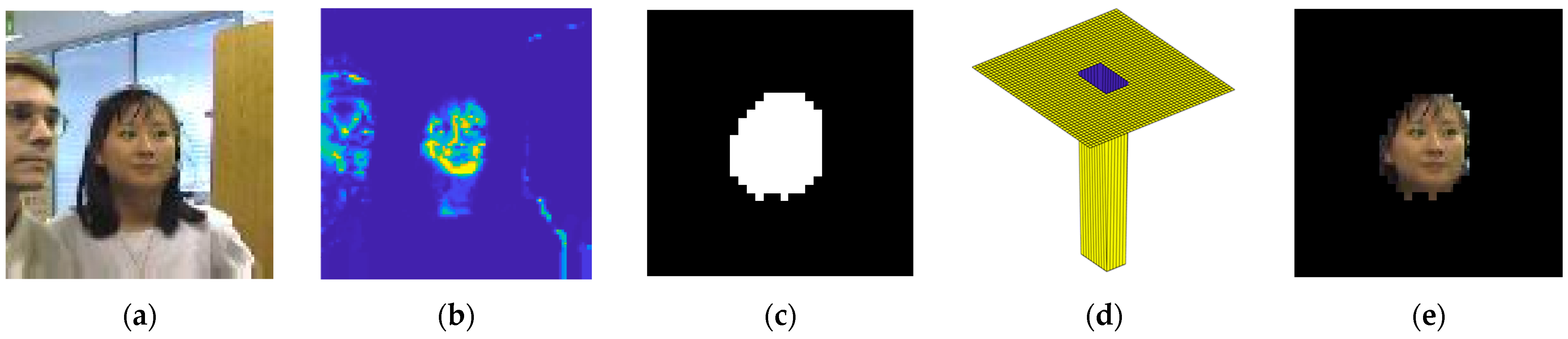
Figure 2 shows the principle of constructing dynamic spatial regularization terms for color histograms, which is mainly divided into three parts: (1) Constructing appearance likelihood probability maps: using foreground color histograms and background color histograms to model the search area separately, obtaining foreground appearance likelihood probability maps and background appearance likelihood probability maps; (2) generating a mask map: combining the appearance likelihood probability map, spatial likelihood probability map, and prior probabilities of foreground and background, using the total probability formula to obtain a posterior probability map representing the foreground, and binarizing it to form a mask map, achieving foreground–background separation; (3) merging the mask image with the static spatial regularization term to generate the dynamic spatial regularization term.

The core of constructing a dynamic spatial regular term for the color histogram is to generate a mask map that fits the appearance of the target. Each pixel point in the mask has a value of $m\in \left\{0,1\right\}$, with $m=1$ indicating that the pixel belongs to the foreground and $m=0$ indicating that the pixel belongs to the background. $m$ takes a value that is related to both the position $x$, where the pixel is located, and the appearance $y$ of the target. The joint probability of each pixel is:

$$p(y,x)={\displaystyle \sum _{i=0}^{1}p(y,x|m=i)p(m=i)}={\displaystyle \sum _{i=0}^{1}p(y|m=i)p(x|m=i)p(m=i)}$$

(5)

where $p(y\mid m=i)$ is the appearance likelihood probability, $p(x\mid m=i)$ is the spatial likelihood probability, and $p(m=i)$ is the prior probability of foreground and background.

(1) Constructing the appearance likelihood probability map: the color histograms $c=\left\{c^f,c^b\right\}$ are extracted for the foreground and background regions, respectively. A symmetric Epanechnikov kernel function is introduced as a spatial prior when counting the foreground color histograms, which is shown in Equation (6):

$$k(r;\sigma )=1-{(r/\sigma )}^2$$

(6)

where $r$ is the distance between the pixel point to be counted and the target center, and $\sigma$ corresponds to the target minimum bounding box. We assign different spatial weights to each pixel value in the target region beforehand; the closer to the target center, the larger the weight, and the farther away from the target center, the smaller the weight. When the pixel to be counted falls in one of the color intervals of the histogram, this weight value is added to the interval instead of plus one. The foreground color histogram is then normalized and back-projected to the search region, i.e., the foreground appearance likelihood probability map $p(y|m=1)$ is obtained. In this way, all pixel points with similar color characteristics to the target will have high probability values and the interferences will be identified. When counting the background color histogram, the pixel points in the target region are not counted, and the remaining pixel points in the search region correspond to the color interval of the color histogram plus one. The background color histogram is then normalized and back-projected to the search interval to obtain a background appearance likelihood probability map $p(y|m=0)$. The background appearance likelihood probability map thus obtained has a lower probability value in the target region.

(2) Generating the mask map: the spatial likelihood probabilities used for foreground and background separation are determined by a modified symmetric Epanechnikov kernel function. The foreground spatial likelihood probability is restricted to the range $\left[0.5,0.9\right]$ such that the prior probability of the target being at the center is 0.9 and the prior probability of being away from the center is 0.5 as shown in Equation (7):

$$p(x|m=1)=k_1(r;\sigma )=\left\{\begin{array}{l}0.9,\hspace{1em}\hspace{1em}\hspace{1em}\hspace{1em}{(r/\sigma )}^2\le 0.1\\ 1-{(r/\sigma )}^2,\hspace{1em}0.1<{(r/\sigma )}^2\le 0.5\\ 0.5,\hspace{1em}\hspace{1em}\hspace{1em}\hspace{1em}0.5<{(r/\sigma )}^2\end{array}\right.$$

(7)

In order to increase the difference between the probability values of the target pixel in the foreground and the background to better highlight the target pixel, the background spatial likelihood probability is restricted to the range $\left[0.1,0.5\right]$ such that the prior probability of the target at the center is 0.1 and that of the target away from the center is 0.5 as shown in Equation (8):

$$p(x|m=0)=k_2(r;\sigma )=\left\{\begin{array}{l}0.1,\hspace{1em}\hspace{1em}\hspace{1em}\hspace{1em}{(r/\sigma )}^2\le 0.1\\ {(r/\sigma )}^2,\hspace{1em}0.1<{(r/\sigma )}^2\le 0.5\\ 0.5,\hspace{1em}\hspace{1em}\hspace{1em}\hspace{1em}0.5<{(r/\sigma )}^2\end{array}\right.$$

(8)

The prior probabilities of foreground and background are determined by the ratio of the area sizes of the extracted target and background histograms. In this paper, we set $p(m=1)=0.38$, $p(m=0)=1.7$. Finally, the posterior probability map of the foreground is obtained from Equation (5), and after binarization processing, a mask $m$ that fits the appearance of the target is obtained, as shown in Figure 2c, achieving foreground–background separation.

(3) Establish dynamic spatial regularization term: Combine the mask $m$ separated from the foreground and background with the static spatial regularization term $w_s$ shown in Figure 2d to suppress pixels that do not belong to the target spatial area or the target appearance area, and obtain the weights of dynamic spatial regularization term $w_r$:

$$w_r=m\odot w_s$$

(9)

In summary, the objective function for constructing the filter is as follows:

$$\epsilon ={\displaystyle \frac{1}{2}}{‖{\displaystyle \sum _{d=1}^D{x}_t^d\star }{f}_t^d-y‖}_2^2+{\displaystyle \frac{1}{2}}{\displaystyle \sum _{d=1}^D{‖w\odot f_t^d‖}_2^2}+{\displaystyle \frac{\lambda }{2}}{‖w-w_r‖}_2^2+{\displaystyle \frac{{\theta }_t}{2}}{\displaystyle \sum _{d=1}^D{‖f_t^d-f_{t-1}^d‖}_2^2+\frac{1}{2}{‖{\theta }_t-\tilde{\theta }‖}_2^2}$$

(10)

In the formula, ${\displaystyle \frac{1}{2}}{\displaystyle \sum _{d=1}^D{‖w\odot f_t^d‖}_2^2}+{\displaystyle \frac{\lambda }{2}}{‖w-w_r‖}_2^2$ is the dynamic spatial regularization term for background suppression, $w_r$ is the reference weight during training, $w$ is the weight to be optimized, and $\lambda$ is the spatial regularization term parameter.

3.3. Algorithm Optimization

The objective function is a convex function of least squares regularization, and the relaxation variable $g=f$ is introduced to construct the original unconstrained optimization problem into a convex optimization problem with equality constraints. The objective function is further written as:

$$\left\{\begin{array}{l}\epsilon ={\displaystyle \frac{1}{2}}{‖{\displaystyle \sum _{d=1}^D{x}_t^d\star }{f}_t^d-y‖}_2^2+{\displaystyle \frac{1}{2}}{\displaystyle \sum _{d=1}^D{‖w\odot g_t^d‖}_2^2}+{\displaystyle \frac{\lambda }{2}}{‖w-w_r‖}_2^2+{\displaystyle \frac{{\theta }_t}{2}}{\displaystyle \sum _{d=1}^D{‖f_t^d-f_{t-1}^d‖}_2^2+\frac{1}{2}{‖{\theta }_t-\tilde{\theta }‖}_2^2}\\ s.t.\mathrm{g}=f\end{array}\right.$$

(11)

The augmented Lagrangian function is:

$$\begin{array}{l}\mathcal{L}(f,g,w,\mu ,s)={\displaystyle \frac{1}{2}}{‖{\displaystyle \sum _{d=1}^D{x}_t^d\star }{f}_t^d-y‖}_2^2+{\displaystyle \frac{1}{2}}{\displaystyle \sum _{d=1}^D{‖w\odot g_t^d‖}_2^2}+{\displaystyle \frac{\lambda }{2}}{‖w-w_r‖}_2^2+{\displaystyle \frac{{\theta }_t}{2}}{\displaystyle \sum _{d=1}^D{‖f_t^d-f_{t-1}^d‖}_2^2}\\ \hspace{1em}\hspace{1em}\hspace{1em}\hspace{1em}\hspace{1em}\hspace{1em}+{\displaystyle \frac{1}{2}}{‖{\theta }_t-\tilde{\theta }‖}_2^2+{\displaystyle \sum _{d=1}^D{(s^d)}^{\top }(f_t^d-g_t^d)+\frac{\rho }{2}{\displaystyle \sum _{d=1}^D{‖f_t^d-g_t^d‖}_2^2}}\end{array}$$

(12)

Among them, $s$ is the Lagrange multiplier and $\rho$ is the step parameter. If $h={\displaystyle \frac{1}{\rho }}s$ is defined as the dual variable of scaling, the above equation can be transformed into:

$$\begin{array}{l}\mathcal{L}(f,g,w,\mu ,h)={\displaystyle \frac{1}{2}}{‖{\displaystyle \sum _{d=1}^D{x}_t^d\star }{f}_t^d-y‖}_2^2+{\displaystyle \frac{1}{2}}{\displaystyle \sum _{d=1}^D{‖w\odot g_t^d‖}_2^2}+{\displaystyle \frac{\lambda }{2}}{‖w-w_r‖}_2^2+{\displaystyle \frac{{\theta }_t}{2}}{\displaystyle \sum _{d=1}^D{‖f_t^d-f_{t-1}^d‖}_2^2}\\ \hspace{1em}\hspace{1em}\hspace{1em}\hspace{1em}\hspace{1em}\hspace{1em}+{\displaystyle \frac{1}{2}}{‖{\theta }_t-\tilde{\theta }‖}_2^2+{\displaystyle \frac{\rho }{2}}{\displaystyle \sum _{d=1}^D{‖f_t^d-g_t^d+h_t^d‖}_2^2}\end{array}$$

(13)

Using the ADMM multiplier method, the above equation can be decomposed into the following subproblems for solution:

$$\left\{\begin{array}{l}{f}^{k+1}=\underset{f}{\arg \min }\left\{{\displaystyle \frac{1}{2}}{‖{\displaystyle \sum _{d=1}^D{x}_t^d\star }{f}_t^d-y‖}_2^2+{\displaystyle \frac{{\theta }_t}{2}}{\displaystyle \sum _{d=1}^D{‖f_t^d-f_{t-1}^d‖}_2^2}+{\displaystyle \frac{\rho }{2}}{\displaystyle \sum _{d=1}^D{‖f_t^d-{(g_t^d)}^k+{(h_t^d)}^k‖}_2^2}\right\}\\ g^{k+1}=\underset{g}{\arg \min }\left\{{\displaystyle \frac{1}{2}}{\displaystyle \sum _{d=1}^D{‖w^k\odot g_t^d‖}_2^2}+{\displaystyle \frac{\rho }{2}}{\displaystyle \sum _{d=1}^D{‖{(f_t^d)}^{k+1}-g_t^d+{(h_t^d)}^k‖}_2^2}\right\}\\ w^{k+1}=\underset{w}{\arg \min }\left\{{\displaystyle \frac{1}{2}}{\displaystyle \sum _{d=1}^D{‖w\odot {(g_t^d)}^{k+1}‖}_2^2}+{\displaystyle \frac{\lambda }{2}}{‖w-w_r‖}_2^2\right\}\\ {\theta }^{k+1}=\underset{\theta }{\arg \min }\left\{{\displaystyle \frac{{\theta }_t}{2}}{\displaystyle \sum _{d=1}^D{‖{(f_t^d)}^{k+1}-{(f_{t-1}^d)}^{k+1}‖}_2^2+\frac{1}{2}{‖{\theta }_t-\tilde{\theta }‖}_2^2}\right\}\\ h^{k+1}=h^k+f^{k+1}-g^{k+1}\end{array}\right.$$

(14)

Among them, $k$ is the number of iterations.

(1) Subproblem $f$: Using the Parseval’s theorem and the convolution theorem, transform it into the Fourier domain:

$$\widehat{f}=\underset{\widehat{f}}{\arg \min }\left\{{\displaystyle \frac{1}{2}}{‖{\displaystyle \sum _{d=1}^D{({\widehat{x}}_t^d)}^{\ast }\odot {\widehat{f}}_t^d-\widehat{y}}‖}_2^2+{\displaystyle \frac{{\theta }_t}{2}}{\displaystyle \sum _{d=1}^D{‖{\widehat{f}}_t^d-{\widehat{f}}_{t-1}^d‖}_2^2}+{\displaystyle \frac{\rho }{2}}{\displaystyle \sum _{d=1}^D{‖{\widehat{f}}_t^d-{\widehat{g}}_t^d+{\widehat{h}}_t^d‖}_2^2}\right\}$$

(15)

Here, for easier explanation, the superscript $k$ is omitted. $\ast$ represents complex conjugation, and $\wedge$ represents discrete Fourier transform (DFT) with symmetry.

It can be observed that the $i\text{-}\mathrm{th}$ row and $j\text{-}\mathrm{th}$ column elements ${\widehat{y}}_{ij}$ of the ideal Gaussian Fourier transform are only related to the $i\text{-}\mathrm{th}$ row and $j\text{-}\mathrm{th}$ column elements ${\widehat{f}}_t\left(i,j\right)$ corresponding to the overall channel and the feature sample ${\widehat{x}}_t^{\ast }\left(i,j\right)$. Let $e_{ij}(\widehat{x})\in {ℂ}^{D\times 1}$, concatenate the ${\widehat{x}}_t^d\left(i,j\right)$ elements on all $D$ channels together, and decompose the above equation into $M\times N$ independent subproblems, each of which takes the form of:

$${\displaystyle \frac{1}{2}}{‖e_{ij}{({\widehat{x}}_t)}^H{e}_{ij}({\widehat{f}}_t)-{\widehat{y}}_{ij}‖}_2^2+{\displaystyle \frac{{\theta }_t}{2}}{‖e_{ij}({\widehat{f}}_t)-e_{ij}({\widehat{f}}_{t-1})‖}_2^2+{\displaystyle \frac{\rho }{2}}{‖e_{ij}({\widehat{f}}_t)-e_{ij}({\widehat{g}}_t)+e_{ij}({\widehat{h}}_t)‖}_2^2$$

(16)

By taking the derivative of $e_{ij}({\widehat{f}}_t)$ and setting it to zero, and taking the identity matrix as $I$, we can obtain the following solution:

$$\left\{\begin{array}{l}q{e}_{ij}({\widehat{f}}_t)=e_{ij}{({\widehat{x}}_t)}^{\ast }{\widehat{y}}_{ij}+{\theta }_t{e}_{ij}({\widehat{f}}_{t-1})+\rho [e_{ij}({\widehat{g}}_t)-e_{ij}({\widehat{h}}_t)]\\ q=e_{ij}{({\widehat{x}}_t)}^{\ast }{e}_{ij}{({\widehat{x}}_t)}^H+\rho +{\theta }_t\end{array}\right.$$

(17)

Since $e_{ij}{({\widehat{x}}_t)}^{\ast }{e}_{ij}{({\widehat{x}}_t)}^H$ is a rank 1 matrix, the Sherman–Morrison formula can be used to solve the above equation:

$$\left\{\begin{array}{l}{e}_{ij}({\widehat{f}}_t)={\displaystyle \frac{1}{\rho +{\theta }_t}}[I-{\displaystyle \frac{e_{ij}{({\widehat{x}}_t)}^{\ast }{e}_{ij}{({\widehat{x}}_t)}^H}{\rho +{\theta }_t+e_{ij}{({\widehat{x}}_t)}^H{e}_{ij}{({\widehat{x}}_t)}^{\ast }}}]p\\ p=e_{ij}{({\widehat{x}}_t)}^{\ast }{\widehat{y}}_{ij}+{\theta }_t{e}_{ij}({\widehat{f}}_{t-1})+\rho [e_{ij}({\widehat{g}}_t)-e_{ij}({\widehat{h}}_t)]\end{array}\right.$$

(18)

(2) Subproblem $g$: Since the subproblem $g$ does not involve convolution operations in the time domain, the derivative of $g$ can be directly set to zero and solved in the time domain. Its closed form solution is:

$$g={\displaystyle \frac{\rho (f+h)}{w\odot w+\rho }}$$

(19)

(3) Subproblem $w$:

$$w={\displaystyle \frac{\lambda w_r}{g\odot g+\lambda }}$$

(20)

(4) Subproblem ${\theta }_t$: Given other variables, the optimal solution for ${\theta }_t$ can be determined as:

$${\theta }_t=\tilde{\theta }-{\displaystyle \frac{{‖f_t-f_{t-1}‖}_2^2}{2}}$$

(21)

(5) Iterative update: In each iteration, $h$ is updated using the last line of Equation (14). Step parameter $\rho$ update:

$$\rho =\min ({\rho }^{\max },\beta {\rho }^k)$$

(22)

Among them, ${\rho }^{\max }$ is the maximum value of $\rho$, and $\beta$ is the step size factor.

3.4. Object Localization and Model Update

Calculate the response map $R_t$ using the obtained optimal filter $f_{t-1}^d$, as shown in Equation (23):

$$R_t={\mathcal{F}}^{-1}({\displaystyle \sum _{d=1}^D{x}_t^d\star }{f}_{t-1}^d)$$

(23)

Among them, ${\mathcal{F}}^{-1}$ is the inverse Fourier transform. The position corresponding to the maximum value of response map $R_t$ is the center of the target. The filter is updated using Equation (24), where ${\eta }_t$ is the learning rate:

$$f_t^d=\left(1-{\eta }_t\right)f_{t-1}^d+{\eta }_t{f}_t^d$$

(24)

The scale estimation of the target is the same as the DSST. A one-dimensional scale filter is trained by extracting multi-scale samples at the target position, and the scale filter obtained from the previous frame is correlated with the scale sample of the current frame to obtain the scale response function. The scale corresponding to the maximum value of the scale response function is the target scale of the current frame.

3.5. Distortion Perception Function

In order to make reliable judgments on the tracking results of the filter, this paper proposes a distortion perception function.

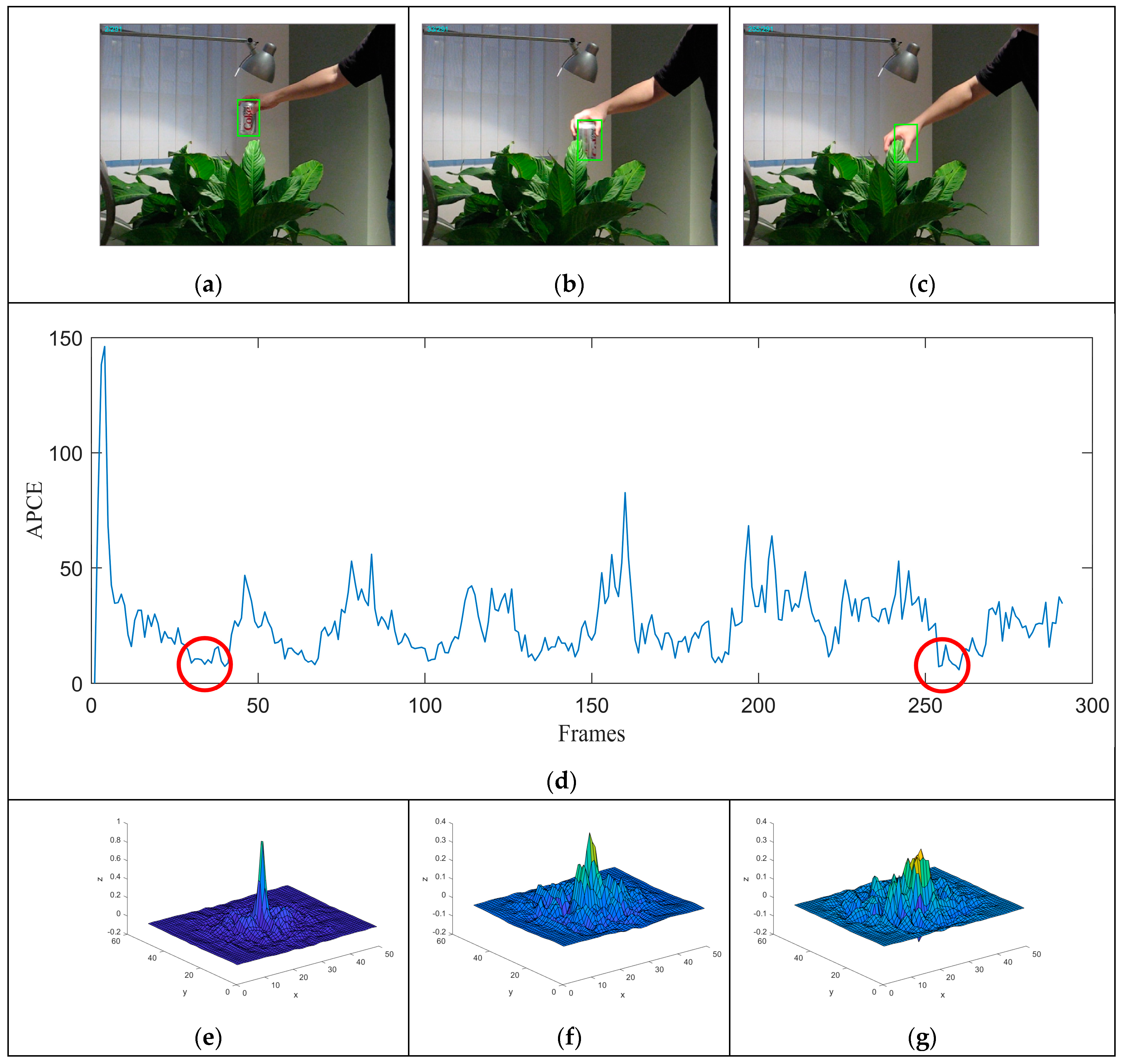
The Average Peak Correlation Energy (APCE) is a commonly used mechanism for measuring the degree of target distortion, which is determined by calculating the global oscillation degree of the response map. The calculation formula is as follows:

$$APCE={\displaystyle \frac{{‖R_{\max }-R_{\min }‖}_2^2}{\left({\displaystyle \sum _{w,h}{(R_{w,h}-R_{\min })}^2}\right)/wh}}$$

(25)

Among them, $R_{\max }$ and $R_{\min }$ represent the maximum and minimum values of the response map, respectively. $R_{i,j}$ is the response value for row $i$ and column $j$. Taking the OTB-100 dataset as an example, Figure 3a–c show the tracking results of frame 2, 33, and 255, corresponding to the states of no distortion, slight distortion, and severe distortion of the target, respectively. Figure 3d shows the variation in APCE values of coke sequences with frames in the OTB-100 dataset. It is not difficult to find that the APCE value is very sensitive to the degree of distortion of the target. The APCE values of the target in the case of slight distortion and severe distortion are very close. Therefore, it is difficult to find a definite threshold to determine the degree of distortion of the target, which can easily lead to misjudgment in some scenarios with low confidence but accurate tracking results.

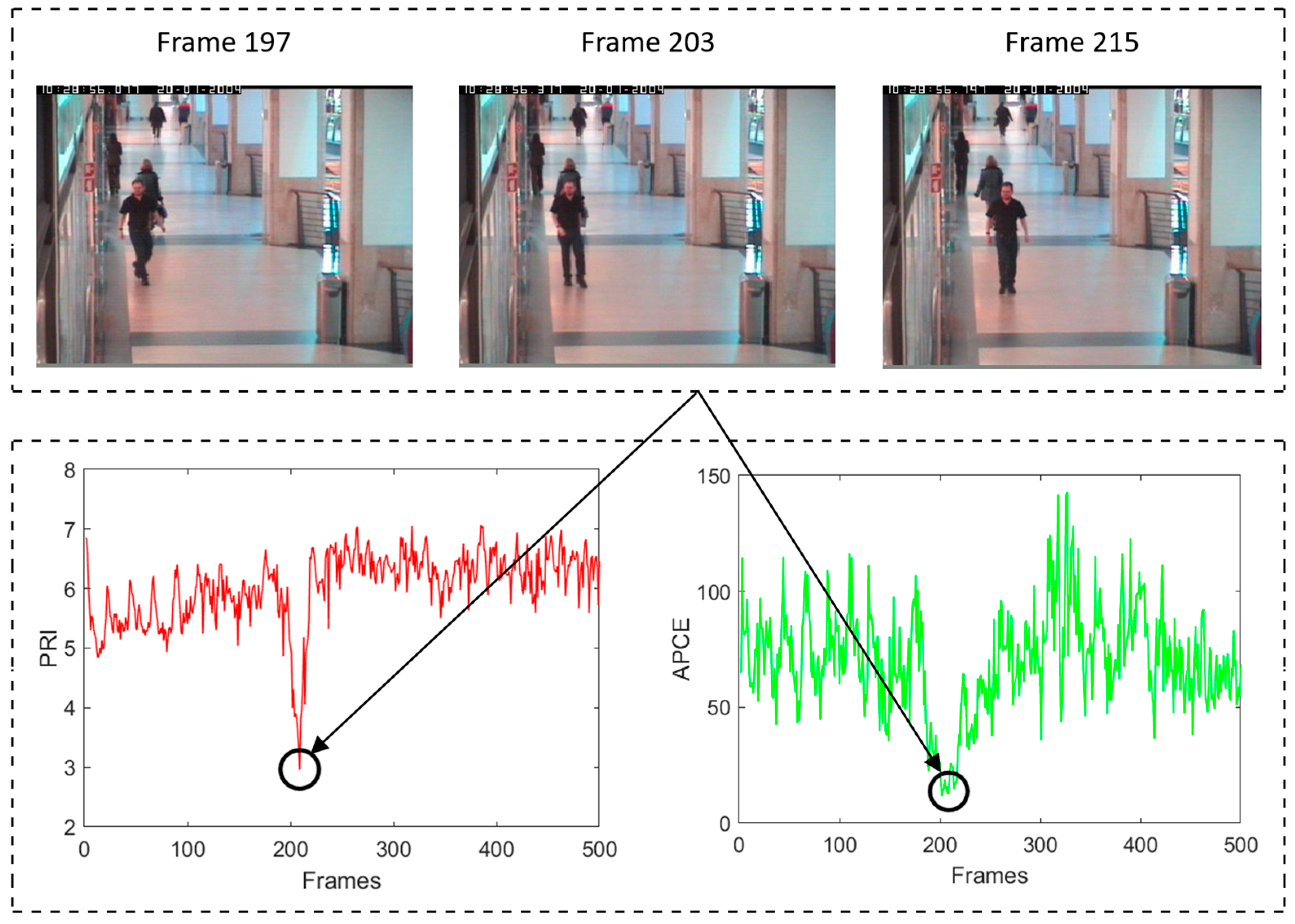
During stable tracking, the main peak of the response map is usually prominent and sharp. Under the influence of occlusion and background clutter, multiple pseudo peaks will appear around the main peak, making it no longer sharp. Figure 3e–g show the response maps of the coke sequence under the conditions of no distortion, slight distortion, and severe distortion of the target, respectively. When the target is in an undistorted state, the response map is a sharp unimodal function of Gaussian shape. When the target is in a slightly distorted state, a secondary peak appears near the main peak in the response map, and the peak value of the main peak decreases and is no longer sharp. When the target is in a severely distorted state, multiple pseudo peaks appear in the response map, and the peak values of the pseudo peaks are slightly higher than those of the main peak, causing the filter to misjudge. Therefore, the sharpness of the main peak in the response map can to some extent reveal the degree of distortion in the tracking results. Based on this, this article proposes the Peak Relative Intensity (PRI) to measure the sharpness of the main peak in the response map:

$$PRI={\displaystyle \frac{F_{\max }-{\mu }_s}{\sigma }}$$

(26)

where $F_{\max }$ is the maximum value of the response map. ${\mu }_s$ and $\sigma$ are the mean and variance of the remaining pixels within the $11\times 11$ window around the peak, except for the peak.

Taking the Walking2 sequence as an example, Figure 4 illustrates the frame variation in the PRI and the APCE. The Walking2 sequence experiences occlusion around frame 203. As shown in the figure, when the target is distorted, both APCE and PRI values show a decreasing trend, with a more significant decrease in the PRI, making it easier to distinguish the distorted state.

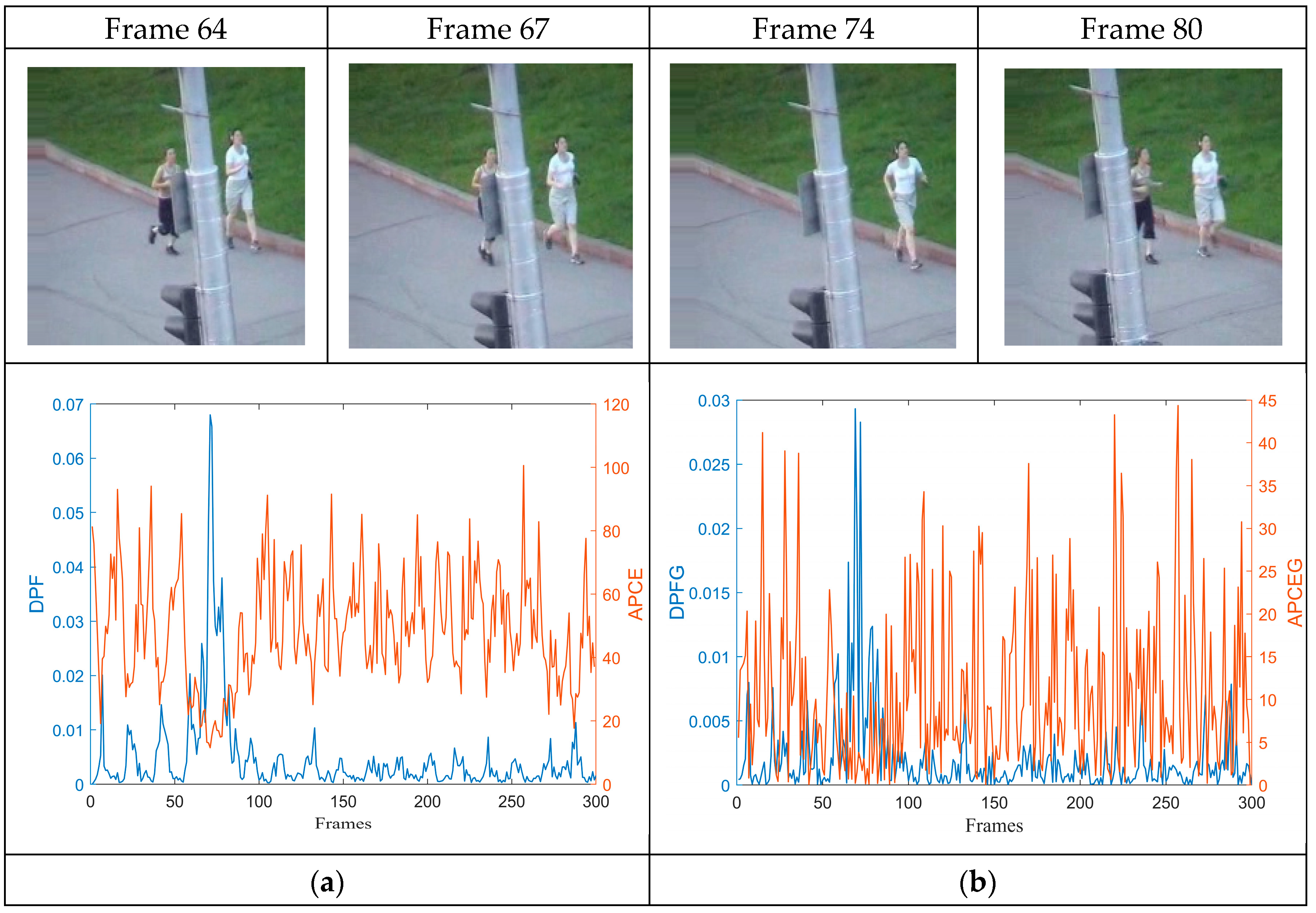
The PRI reflects the degree of local oscillation in the response map and focuses more on the target and its surrounding environment, making it more sensitive to deformation, occlusion, and other situations; the APCE reflects the degree of global oscillation in the response map and focuses more on the global environment of the search area, making it more sensitive to lighting conditions, rapid motion, and other situations. Based on this, this article proposes a distortion perception function (DPF) that combines PRI and APCE values, and is more comprehensive and accurate to determine the degree of distortion of the target. The DPF is defined as:

$$DPF=APC{E}^{-{\log }_{10}(PRI)}$$

(27)

Table 1. Analysis of APCE, PRI, and DPF values.

Evaluating Indicator	APCE	PRI	DPF
Meaning	Measure the reliability of the current frame tracking result based on the global oscillation degree of the response map (the bigger, the better)	Measure the distortion level of the current frame object based on the sharpness of the main peak in the response map (the bigger, the better)	Measure the distortion level of the current frame object (the smaller, the better)
Theoretical Value	≥0	≥0	>0
Experimental Value	3~327	1~11	2 × 10−6~0.9

shows the meanings and ranges of APCE, PRI, and DPF values. From this table, it can be seen that there is a significant difference in the range of values between the APCE and PRI. In order to highlight the difference in amplitude corresponding to different degrees of distortion of the target, this paper combines the two in an exponential manner.

For the convenience of comparison, taking the joking1 sequence as an example, the numerical changes in the DPF and the APCE are compared, as shown in Figure 5. It can be observed that compared to the sensitivity of APCE values to the degree of target distortion, the DPF is only higher and accompanied by significant fluctuations when the target undergoes severe distortion due to severe occlusion, while the rest of the frame changes relatively smoothly.

In order to demonstrate more clearly that the DPF can effectively determine the degree of target distortion, taking the first 500 frames of the Girl2 sequence as an example, the variation in DPF values with frames and the degree of target distortion are visualized, as shown in Figure 6. The target experiences similar background interference around frame 55, partial occlusion around frame 106, complete occlusion around frame 110, and deformation around frame 280. The DPF corresponding to several situations vary greatly, and the DPF value is highest when the target undergoes severe distortion due to occlusion.

This article assumes that when the condition $DPF>{\theta }_1$ is met, the current frame target is in a severely distorted state, and the tracking results are unreliable.

3.6. Kalman Filter Tracking

The Kalman filter [11] is an efficient recursive estimation method that utilizes prior knowledge and observation data of the system to make optimal estimates of the system state in the presence of noise. In this article, when the tracking results of the target are unreliable due to severe distortion, we use a Kalman filter to predict the tracking results. The state equation and observation equation of the Kalman filter can be expressed as:

$$x_t=A_{t,t-1}{x}_{t,t-1}+w_{t-1}$$

(28)

$$y_t=H_t{x}_t+v_t$$

(29)

where $x_t$ and $x_{t-1}$ represent the states of frame $t$ and $t-1$, respectively, which can be described as $x_t=[x,y,v_x,v_y]$, where $(x,y)$ represents the center position of the target. $v_x$ and $v_y$ represent the horizontal and vertical velocities.$A_{t,t-1}$ represents the state transition matrix from frame $t-1$ to $t$, $y_t$ is the observation vector, and $H_t$ represents the observation matrix. Since the Kalman filter only serves as a correction in DADSTRCF, this paper assumes that the motion model of the target between adjacent frames is a uniform linear motion. When using the Kalman filter for target tracking, the target is treated as a point. Therefore, the state transition and measurement matrix are defined as:

$$A_{t,t-1}=\left[\begin{array}{cccc}1& 0& \Delta t& 0\\ 0& 1& 0& \Delta t\\ 0& 0& 1& 0\\ 0& 0& 0& 1\end{array}\right]$$

(30)

$$H_t=\left[\begin{array}{cccc}1& 0& 0& 0\\ 0& 1& 0& 0\end{array}\right]$$

(31)

$w_{t-1}$ and $v_t$, respectively, represent process noise and measurement noise, both of which follow normal distributions with covariance matrices Q and R, respectively.

The true value, predicted value, and optimal estimated value of the target in frame $t$ are represented as $x_t$, $x_t^{-}$, ${\tilde{x}}_t$. The prediction error covariance matrix and estimation error covariance matrix of the Kalman filter are defined as:

$$S_t^{-}=E[e_k^{\prime }{e_k^{\prime }}^{⊺}]=E[(x_t-x_t^{-}){(x_t-x_t^{-})}^{⊺}]$$

(32)

$$S_t=E[e_k{e}_k^{⊺}]=E[(x_t-{\tilde{x}}_t){(x_t-{\tilde{x}}_t)}^{⊺}]$$

(33)

Kalman filtering mainly includes two parts: prediction and correction.

(1)

Prediction section:

The prediction part mainly includes state prediction and error covariance matrix prediction. They are, respectively, expressed as:

$$x_t^{-}=A_{t,t-1}{\tilde{x}}_{t-1}$$

(34)

$$S_t^{-}=A_{t,t-1}{S}_{t-1}{A}_{t,t-1}^{\top }+Q$$

(35)

(2)

Correction section:

The correction part mainly includes state correction, Kalman gain correction, and error covariance correction. They are, respectively, expressed as:

$$K_t=S_t^{-}{H}^{\top }{(H{S}_t^{-}{H}^{\top }+R)}^{-1}$$

(36)

$${\tilde{x}}_t=x_t^{-}+K_t(y_t-H_t{x}_k^{-})$$

(37)

$$S_t=(I-K_{t}H)S_t^{-}$$

(38)

where $K_t$ is the Kalman gain.

4. Experiments

This section provides a detailed presentation and analysis of the experimental details and results. Firstly, the experimental details, experimental dataset, and evaluation indicators were introduced. Then, quantitative comparisons were made with various DCF tracking algorithms on the selected dataset. Next, the superiority of the tracker was visually demonstrated through qualitative analysis. Finally, the effectiveness of each module of DADSTRCF was verified through ablation experiments.

4.1. Experimental Details and Parameters

All experiments are implemented in Matlab R2021a and run on a PC equipped with an Inter (R) Core (TM) i7-12700H CPU@2.30 GHz, 16GB RAM.

In the experiment, the spatial regularization coefficient in the objective function is set to $\lambda =1.0$, the adaptive time regularization coefficient is set to $\nu =2\times {10}^{-5}$, $\zeta =15$, $\varphi =3000$, the ADMM iteration number is set to 2, the initial value of the step parameter $\rho$ is set to ${\rho }_0=1$, the maximum value is set to ${\rho }^{\max }=1000$, the step size factor is set to $\beta =10$, and the learning rate in the model update is set to ${\eta }_t=0.0193$. The DPF threshold is set to ${\theta }_1=0.1$. In the Kalman filter, $\Delta t=1$, $Q=0.1I$, and $R=I$, $I$ is the identity matrix.

4.2. The Dataset and Evaluation Metrics

4.2.1. The Dataset

To verify the effectiveness of the algorithm proposed in this paper, the public datasets OTB-50 [57], OTB-100 [39], UAV123 [58], and DTB70 [59] were used to test and analyze the algorithm.

The OTB-50 dataset consists of 50 image sequences, including 11 challenges: background clutter (BC), scale variation (SV), occlusion (OCC), deformation (DEF), illumination variation (IV), low resolution (LR), out of view (OV), motion blur (MB), fast motion (FM), in-plane rotation (IPR), and out-of-plane rotation (OPR). The OTB-100 dataset is an extension of OTB-50, which adds different types of targets, different motion patterns, and different environmental conditions, covering a wider range of scenarios. The OTB dataset is a universal benchmark dataset in the field of object tracking, which can evaluate the performance of object tracking algorithms under different attributes.

The UAV123 dataset contains 123 image sequences and has added aspect ratio change (ARC), similar object interference (SOB), and viewpoint change (VC) attributes compared to the OTB dataset. The occlusion attributes are further subdivided into full occlusion (FOC) and partial occlusion (POC) attributes. The DTB70 dataset contains 70 image sequences, with targets exhibiting diverse motion patterns and appearance changes. UAV123 and DTB70 are commonly used in the field of unmanned aerial vehicle tracking and have higher complexity, making them important benchmarks for evaluating the tracking performance of algorithms in complex scenarios.

4.2.2. Evaluation Metrics

The experiment used the One Pass Evaluation (OPE) [59] criterion from the OTB dataset as the evaluation scheme, and measured the performance of each candidate tracker on four datasets using its success rate curve area under the ROC curve (AUC) and distance precision (DP).

The success rate indicator is based on the intersection-over-union (IoU) ratio between the predicted bounding box and the actual bounding box. The success rate is defined as the percentage of frames with IoU exceeding a given threshold, formulated as:

$$OP={\displaystyle \frac{1}{N}}{\displaystyle \sum _{i=1}^N{S}_i}$$

(39)

$$S_i=\left\{\begin{array}{l}1\hspace{1em}\hspace{1em}IoU\ge Tr\\ 0\hspace{1em}\hspace{1em}IoU<Tr\end{array}\right.$$

(40)

$$IoU={\displaystyle \frac{Area(B_{pr}\cap B_{gt})}{Area(B_{pr}\cup B_{gt})}}$$

(41)

Among them, $N$ represents the total number of frames in the video sequence, $S_i$ represents whether the current frame is successfully tracked, $B_{pr}$ and $B_{gt}$ represent the predicted bounding box and the real bounding box, respectively, and the symbol $\cap \cup$ represents the intersection and union of the two elements. $T_r$ is a given threshold, and we can take different thresholds between 0 and 1 to plot the success rate curve. Then, we use AUC to rank the trackers.

Precision is defined as the proportion of video frames in a video sequence where the Euclidean distance between the predicted target center and the true target center position is less than a given threshold. Precision can be expressed as:

$$DP={\displaystyle \frac{1}{N}}{\displaystyle \sum _{i=1}^N{P}_i}$$

(42)

$$P_i=\left\{\begin{array}{l}1\hspace{1em}\hspace{1em}CLE\le d\\ 0\hspace{1em}\hspace{1em}CLE>d\end{array}\right.$$

(43)

$$CLE=\sqrt{{(x_{pr}-x_{gt})}^2-{(y_{pr}-y_{gt})}^2}$$

(44)

where $P_i$ represents whether the current center position error is less than a given threshold, and $(x_{pr},y_{pr})$ and $(x_{gt},y_{gt})$ represent the predicted and true target centers, respectively. $CLE$ represents the center position error. $D$ is a given threshold. Use a common threshold of 20 pixels in the experiment to rank the tracker.

4.3. Experimental Results and Analysis

This section compares DADSTRCF with various advanced correlation filtering target tracking algorithms and provides a detailed analysis, including both quantitative comparison and qualitative analysis.

4.3.1. Quantitative Comparison

We select nine representative correlated filtering trackers for comparative experiments from the aspects of feature representation (FR), scale estimation (SE), dynamic spatial regularization (DSR), dynamic temporal regularization (DTR), distortion perception functions (DPFs), baseline (B), etc., including BACFs [37], STRCF [38], SRDCFs [36], CSR-DCF [49], DRCF [46], Auto Track [7], Staple [48], EFSCF [60], and SOCF [61]. Specific details are shown in

Table 2. Anti-occlusion correlation filter based on background suppression and comparative tracker for distortion perception.

Tracker	FR	SE	DSR	DTR	DPF	B
DADSTRCF	gray+HOG+CN	Yes	Yes	Yes	Yes	Auto Track
Auto Track	gray+HOG+CN	Yes	Yes	Yes	No	STRCF
CSR-DCF	gray+HOG+CN	Yes	Yes	No	No	KCF
DRCF	gray+HOG+CN	Yes	Yes	No	No	SRDCF
EFSCF	gray+HOG+CN	Yes	No	No	No	STRCF
SOCF	gray+HOG+CN	Yes	No	No	No	STRCF
STRCF	gray+HOG+CN	Yes	No	No	No	SRDCF
SRDCF	gray+HOG+CN	Yes	No	No	No	KCF
Staple	HOG+CH	Yes	No	No	No	KCF
BACF	HOG	Yes	No	No	No	MOSSE

. And the distance precision curves and success rate curves of 10 algorithms on 4 datasets are shown in Figure 7.

As shown in Figure 7, DADSTRCF achieves the highest DP score and AUC score. Specifically, on the OTB-50, the DP score of DADSTRCF (89.8%) exceeded the baseline Auto Track (83.5%) and the second highest tracker STRCF (89.6%), with improvements of 6.3% and 0.2%, respectively. Meanwhile, the AUC score of DADSTRCF (87.2%) is also better than the baseline Auto Track (77.9%) and the second highest tracker EFSCF (86.8%), with improvements of 9.3% and 0.4%, respectively. On the OTB-100, the DP score of DADSTRCF (87.3%) exceeded the baseline Auto Track (78.9%) and the second highest tracker EFSCF (86.6%), with improvements of 8.4% and 0.7%, respectively. The AUC score of DADSTRCF (82.3%) has increased by 9.3% and 1.4%, respectively, compared to the baseline Auto Track (71.9%) and the second highest tracker EFSCF (80.9%).

On the UAV123, the DP score of DADSTRCF (70.1%) improved by 2.0% and 0.8%, respectively, compared to the baseline Auto Track (68.1%) and the second highest tracker EFSCF (69.3%). The AUC score of DADSTRCF (58.0%) increased by 2.5% and 0.9%, respectively, compared to baseline Auto Track (55.5%) and the second highest tracker EFSCF (57.1%). On DTB70, the DP score of DADSTRCF (71.6%) improved by 6.4% and 5.5%, respectively, compared to the baseline Auto Track (65.2%) and the second highest tracker SOCF (66.6%). The AUC score of DADSTRCF (47.8%) has increased by 3.9% and 3.0%, respectively, compared to the baseline algorithm Auto Track (43.9%) and the second highest tracker SOCF (44.8%).

It is worth mentioning that the UAV datasets UAV123 and DTB70 pose more challenges than the general datasets OTB. This is because unmanned aerial vehicles, due to their strong maneuverability and flexible movements, often face more complex and variable backgrounds, and the appearance of targets is more prone to distortion. This also explains why most trackers have lower precision and success rates on UAV datasets. DADSTRCF not only shows significant improvements in the DP and AUC scores compared to the baseline Auto Track in UAV datasets, especially the DTB70, but also has considerable advantages over the second highest tracker. This is because DADSTRCF introduces a dynamic spatial regularization term based on color histograms, which can better suppress background clutter and similar interferences in complex scenes. In addition, the distortion perception function of DADSTRCF can supervise the degree of distortion in the appearance of the target, and timely adopt a Kalman tracker to correct the tracking results, thus better coping with complex and changing scenes.

Table 3. DP scores of 10 algorithms on partial attributes of the OTB-50 dataset.

Attribute	Ours	STRCF	BACF	SRDCF	CSRDCF	DRCF	Auto Track	Staple	EFSCF	SOCF
OPR	0.892 1	0.891	0.811	0.863	0.809	0.776	0.824	0.752	0.885	0.840
OCC	0.917	0.916	0.852	0.872	0.838	0.755	0.835	0.738	0.908	0.852
DEF	0.924	0.923	0.879	0.880	0.823	0.830	0.897	0.817	0.923	0.847
IPR	0.915	0.914	0.851	0.811	0.842	0.811	0.814	0.756	0.908	0.849
OV	0.956	0.952	0.914	0.874	0.848	0.799	0.824	0.748	0.906	0.902
BC	0.902	0.899	0.823	0.816	0.851	0.812	0.808	0.748	0.880	0.817

¹ The data ranked first in each attribute in the table is represented in red, while the data ranked second and third are represented in green and blue.

and

Table 4. AUC scores of 10 algorithms on partial attributes of the OTB-50 dataset.

Attribute	Ours	STRCF	BACF	SRDCF	CSRDCF	DRCF	Auto Track	Staple	EFSCF	SOCF
OPR	0.864 1	0.835	0.779	0.786	0.750	0.737	0.743	0.694	0.861	0.787
OCC	0.880	0.877	0.814	0.800	0.757	0.714	0.740	0.672	0.877	0.790
DEF	0.919	0.917	0.880	0.867	0.812	0.814	0.850	0.785	0.918	0.813
IPR	0.888	0.854	0.827	0.747	0.787	0.785	0.761	0.719	0.884	0.829
OV	0.947	0.945	0.873	0.798	0.758	0.742	0.713	0.629	0.902	0.779
BC	0.881	0.831	0.743	0.730	0.764	0.763	0.741	0.682	0.859	0.760

¹ The data ranked first in each attribute in the table is represented in red, while the data ranked second and third are represented in green and blue.

quantitatively demonstrate the DP score and AUC score of 10 DCF trackers under certain attributes in the OTB-50. Compared with Auto Track, under the background clutter attribute, the DP score and AUC score of DADSTRCF have been improved by 9.4% and 14.0%, respectively. This is due to the improved dynamic spatial regularization term of DADSTRCF, which can focus on the target during tracking and suppress interference in the background. Under the out of plane rotation attribute, the DP score and AUC score of DADSTRCF increased by 6.8% and 12.1%, respectively. Under the occlusion attribute, the DP score and AUC score of DADSTRCF increased by 8.2% and 14%, respectively. Under the rotation attribute in the plane, the DP score and AUC score of DADSTRCF increased by 10.1% and 12.7%, respectively. On the one hand, this is largely attributed to the distortion perception function proposed in this paper, which enables the filter to accurately judge the reliability of tracking results and timely use the Kalman tracker for prediction when tracking is inaccurate. On the other hand, since the dynamic spatial regularization term of DADSTRCF is based on color histograms, and color feature is not sensitive to deformation, rotation, etc., it also improves the tracking performance of DADSTRCF, when it is under deformation, rotation, and other attributes. In addition, during the experiments, we found that DADSTRCF has significantly improved performance in out of view, with the DP score and AUC score increasing by 13.2% and 23.4%, respectively. From another perspective, out of the view can also be seen as a special case of target severe distortion, which indirectly confirms the effectiveness of distortion perception functions and Kalman trackers.

Table 5. DP scores of 10 algorithms on partial attributes of the UAV123 dataset.

Attribute	Ours	STRCF	BACF	SRDCF	CSRDCF	DRCF	Auto Track	Staple	EFSCF	SOCF
POC	0.622 1	0.587	0.564	0.608	0.566	0.587	0.584	0.571	0.617	0.574
BC	0.591	0.502	0.513	0.526	0.571	0.541	0.584	0.517	0.532	0.523
VC	0.625	0.581	0.587	0.593	0.607	0.583	0.618	0.604	0.596	0.596
SOB	0.719	0.648	0.673	0.678	0.640	0.652	0.666	0.670	0.717	0.690

¹ The data ranked first in each attribute in the table is represented in red, while the data ranked second and third are represented in green and blue.

shows the DP score of 10 algorithms on some attributes of UAV123. The performance of DADSTRCF is optimal under local occlusion, background clutter, viewpoint change, and similar object interference attributes. Compared with Auto Track, the DP score of our algorithm increased by 3.8% under local occlusion attributes and 5.3% under similar object interference attributes.

Table 6. DP scores of 10 algorithms on partial attributes of the DTB70 dataset.

Attribute	Ours	STRCF	BACF	SRDCF	CSRDCF	DRCF	Auto Track	Staple	EFSCF	SOCF
OCC	0.631 1	0.617	0.515	0.478	0.585	0.587	0.628	0.528	0.617	0.631
IPR	0.684	0.586	0.534	0.419	0.584	0.584	0.579	0.457	0.587	0.604
OV	0.690	0.652	0.567	0.552	0.629	0.558	0.593	0.420	0.652	0.669
BC	0.635	0.611	0.499	0.393	0.602	0.551	0.566	0.393	0.623	0.623
SOB	0.731	0.677	0.624	0.569	0.637	0.676	0.715	0.529	0.663	0.730

¹ The data ranked first in each attribute in the table is represented in red, while the data ranked second and third are represented in green and blue.

shows the DP score of 10 algorithms on some attributes of DTB70. DADSTRCF is optimal under attributes such as occlusion, in-plane rotation, out of view, background clutter, and interference from similar objects.

4.3.2. Qualitative Analysis

In order to obtain a more intuitive comparison, qualitative evaluation results of DADSTRCF and comparison algorithms are presented on five challenging image sequences, as shown in Figure 8. These sequences include various challenges such as background clutter (Gulf, Motor, Soccer), fast motion (Gulf, DragonBaby), in-plane rotation and out of plane rotation (Gulf, DragonBaby, Motor), similar object interference (Gulf, DragonBaby, Soccer), and occlusion (joking-1, DragonBaby, Soccer). DADSTRCF exhibits excellent performance in these sequences.

In the sequence Gulf, the target undergoes significant out of plane rotation while moving rapidly, causing other trackers to drift quickly during the tracking process, resulting in tracking failure. Due to its distortion perception function, DADSTRCF can use Kalman filter to correct tracking results in a timely manner when tracking is inaccurate, thus enabling continuous and stable tracking of targets. The same situation also occurs in the sequence Motor and DragonBaby. In these sequences, the target undergoes severe distortion due to out of plane rotation, causing a certain degree of drift in all tracking frames. However, DADSTRCF has the lightest drift and best fits the target because it can use a Kalman tracker to correct the results.

In the sequence joking-1, the target is severely occluded at frame 72. When the target reappears in the field of view, only DADSTRCF and BACFs can perform stable tracking, but the result of DADSTRCF is more accurate. This is not only due to the dynamic spatial regularization term based on color histograms, which makes DADSTRCF a more robust model than BACFs, but also thanks to the integrated Kalman tracker in the DCF framework, which can correct tracking results in real time.

In the sequence Soccer, the target undergoes out of plane rotation around frame 78, causing significant distortion. At this point, only DADSTRCF and Auto Track can stably track the target, while other trackers experience significant drift. At frame 140, there is severe background clutter around the target, and DADSTRCF can consistently track the target due to its ability to suppress interference clutter with similar features. At frame 180, the target experienced background clutter, similar object interference, and complete occlusion simultaneously, causing all trackers to drift. However, DADSTRCF experienced slight drift due to the effect of the Kalman tracker. At 290 frame, as the target gradually becomes clearer, both DADSTRCF and EFSCF retrack on the target, with DADSTRCF has a more accurate result, proving its superior performance in complex scenes.

4.4. Ablation Experiment

In this section, we conducted ablation experiments to demonstrate the effectiveness of each module in DADSTRCF. We use “DSR” to represent the dynamic spatial regularization term based on color histograms, and “DPF” to represent the distortion perception function. The experimental results are shown in

Table 7. Results of ablation experiments on the OTB-100 dataset.

Algorithm	DSR	DPF	DP	AUC
Auto Track (Baseline)	No	No	0.789	0.719
Baseline+DSR	Yes	No	0.866	0.803
DADSTRCF (Ours)	Yes	Yes	0.873	0.812

. According to Table 7, each module can improve the performance of the tracker. Among them, the dynamic spatial regularization term based on color histogram increased the baseline algorithm’s DP score and AUC score by 7.7% and 8.4%, respectively, while the introduction of distortion perception function further improved the DP score and AUC score by 0.7% and 0.9%, respectively.

From the above analysis, it can be seen that each improved module of the algorithm in this article has improved the tracking performance, indicating the effectiveness of the algorithm in this article.

5. Conclusions

When facing scenarios such as background clutter and interference from similar objects, DCF trackers are prone to drift or tracking failure. To address this issue, this paper proposes a distortion-aware dynamic spatial–temporal regularization correlated filtering (DADSTRCF) target tracking algorithm. DADSTRCF utilizes color histograms to construct dynamic spatial regularization terms, and proposes a distortion perception function (DPF) to determine the reliability of tracking results. When the tracking results are unreliable, the Kalman filter is used to predict in a timely manner, effectively alleviating the effects of background clutter, similar interferences, and boundary effects, enhancing the robustness and adaptability of the filter, and significantly reducing the risk of model drift or even tracking failure. Comparative experiments were conducted on the OTB-50, OTB-100, UAV123, and DTB70 datasets, and the experimental results showed that DADSTRCF had the highest DP score and AUC score on all four datasets, with improvements of (6.3%, 9.3%), (8.4%, 9.3%), (2.0%, 2.5%), and (6.4%, 3.9%) compared to Auto Track, respectively. Under similar background interference, background clutter, occlusion and other attributes, the tracking performance of DADSTRCF is significantly better than other trackers, fully demonstrating the superiority of DADSTRCF.

However, during the experiments, it was found that DP scores of DADSTRCF in low resolution and other scenarios lack competitiveness. Given the limited representation capability of handcrafted features, future work will explore the integration of deep features with handcrafted features, aiming to enhance tracking performance without compromising real-time efficiency. In addition, the fixed model update strategy limits the adaptability of tracker to complex scenes, and increases the risk of model drift. Therefore, the next step is to combine the distortion perception function with the model update mechanism to achieve adaptive model update.

References

1. Zhang, J.; Zhang, X.; Huang, Z.; Cheng, X.; Feng, J.; Jiao, L. Bidirectional Multiple Object Tracking Based on Trajectory Criteria in Satellite Videos. IEEE Trans. Geosci. Remote Sens. 2023, 61, 5603714. [Google Scholar] [CrossRef]
2. Siddharth, R.; Aghila, G. A Fog-Assisted Framework for Intelligent Video Preprocessing in Cloud-based Video Surveillance as a Service. IEEE Trans. Sustain. Comput. 2022, 7, 825–838. [Google Scholar]
3. Bu, Y.; Xie, L.; Gong, Y.; Wang, C.; Yang, L.; Liu, J.; Lu, S. RF-Dial: Rigid Motion Tracking and Touch Gesture Detection for Interaction via RFID Tags. IEEE Trans. Mob. Comput. 2022, 21, 1061–1080. [Google Scholar] [CrossRef]
4. James, R.; Nosib, H. Fast-Track, rapid-access pathways for the diagnosis of gynaecological cancers. Obstet. Gynaecol. Reprod. Med. 2024, 34, 134–143. [Google Scholar] [CrossRef]
5. Stodola, P. Improvement in the model of cooperative aerial reconnaissance used in the tactical decision support system. J. Def. Model. Simul. 2017, 14, 483–492. [Google Scholar] [CrossRef]
6. Mu, L.; Xie, G.; Yu, X.; Wang, B.; Zhang, Y. Robust Guidance for a Reusable Launch Vehicle in Terminal Phase. IEEE Trans. Aerosp. Electron. Syst. 2022, 58, 1996–2011. [Google Scholar] [CrossRef]
7. Li, Y.; Fu, C.; Ding, F.; Huang, Z.; Lu, G. AutoTrack: Towards High-Performance Visual Tracking for UAV with Automatic Spatio-Temporal Regularization. In Proceedings of the IEEE/CVF Conference on Computer Vision and Pattern Recognition (CVPR), Seattle, WA, USA, 13 June 2020. [Google Scholar]
8. Luo, W.; Biao, L.I.; Ruigang, F. Infrared Ground Multi-object Tracking Method Based on Improved ByteTrack Algorithm. Comput. Sci. 2023, 50, 176–183. [Google Scholar]
9. Lucas, B.D.; Kanade, T. An Iterative Image Registration Technique with an Application to Stereo Vision. In Proceedings of the 7th International Joint Conference on Artificial Intelligence, Vancouver, BC, Canada, 24–28 August 1981; pp. 674–679. [Google Scholar]
10. Zhu, S.; Yang, S.; Hu, P.; Qu, X. A Robust Optical Flow Tracking Method Based on Prediction Model for Visual-Inertial Odometry. IEEE Robot. Autom. Lett. 2021, 6, 5581–5588. [Google Scholar] [CrossRef]
11. Kalman, R.E. A New Approach to Linear Filtering and Prediction Problems. J. Fluids Eng. 1960, 82, 35–45. [Google Scholar] [CrossRef]
12. Sahoo, S.R.; Mannivanan, P.V. A Novel Method for Ground Vehicle Tracking with Error-State Kalman Filter Based Visual-LiDAR Odometry (ESKF-VLO); IEEE Access: Piscataway, NJ, USA, 2024; Volume 12. [Google Scholar]
13. Li, J.; Xu, X.; Jiang, Z.; Jiang, B. Adaptive Kalman Filter for Real-Time Visual Object Tracking Based on Autocovariance Least Square Estimation. Appl. Sci. 2024, 14, 1045. [Google Scholar] [CrossRef]
14. Comaniciu, D.; Ramesh, V.; Meer, P. Real-Time tracking of non-rigid objects using mean shift. In Proceedings of the IEEE Conference on Computer Vision and Pattern Recognition, Hilton Head Island, SC, USA, 15 June 2000; Volume 2. [Google Scholar]
15. Wang, Z.; Yang, X.; Xu, Y.; Yu, S. CamShift guided particle filter for visual tracking. Pattern Recognit. Lett. 2009, 30, 407–413. [Google Scholar] [CrossRef]
16. Li, J.; Tian, Y.; Guo, M.; Zuo, K.; Wang, X. Visual group target tracking algorithm based on MeanShift-PCA-PF. In Proceedings of the 8th International Conference on Intelligent Computing and Signal Processing (ICSP), Xi’an, China, 21–23 April 2023. [Google Scholar]
17. Black, M.J.; Jepson, A.D. EigenTracking: Robust matching and tracking of articulated objects using a view-based representation. Int. J. Comput. Vis. 1998, 26, 63–84. [Google Scholar] [CrossRef]
18. Javed, S.; Mahmood, A.; Ullah, I.; Bouwmans, T.; Khonji, M.; Dias, J.M.M.; Werghi, N. A Novel Algorithm Based on a Common Subspace Fusion for Visual Object Tracking; IEEE Access: Piscataway, NJ, USA, 2022; Volume 10, pp. 24690–24703. [Google Scholar]
19. Sui, Y.; Wang, G.; Zhang, L. In Defense of Subspace Tracker: Orthogonal Embedding for Visual Tracking. arXiv 2022, arXiv:2204.07927. [Google Scholar]
20. Tao, R.; Gavves, E.; Smeulders, A.W.M. Siamese Instance Search for Tracking. In Proceedings of the EEE Conference on Computer Vision and Pattern Recognition (CVPR), Las Vegas, NV, USA, 27–30 June 2016. [Google Scholar]
21. Sun, Y.; Tang, C.; Luo, H.; Li, Q.; Peng, X.; Zhang, J.; Li, M.; Wei, Y. Joint spatio-temporal modeling for visual tracking. Knowl.-Based Syst. 2024, 283, 111206. [Google Scholar] [CrossRef]
22. Yu, P.; Duan, Z.; Guan, S.; Li, M.; Deng, S. UnifiedTT: Visual tracking with unified transformer. J. Vis. Commun. Image Represent. 2024, 99, 104067. [Google Scholar] [CrossRef]
23. Yang, K.; Li, Q.; Tian, C.; Zhang, H.; Shi, A.; Li, J. DeforT: Deformable transformer for visual tracking. Neural Netw. 2024, 176, 106380. [Google Scholar] [CrossRef]
24. Wang, J.; Ye, X.; Wu, D.; Gong, J.; Tang, X.; Li, Z. Evolution of Siamese Visual Tracking with Slot Attention. Electronics 2024, 13, 586. [Google Scholar] [CrossRef]
25. Liu, K.; Liu, L.; Yang, S.; Fu, Z. Spatial feature embedding for robust visual object tracking. IET Comput. Vis. 2024, 18, 540–556. [Google Scholar] [CrossRef]
26. Tang, C.; Wang, K.; van de Weijer, J.; Zhang, J.; Huang, Y. AViTMP: A Tracking-Specific Transformer for Single-Branch Visual Tracking. IEEE Trans. Intell. Veh. 2024, 1–14. [Google Scholar] [CrossRef]
27. Wu, R.; Liu, Y.; Wang, X.; Yang, P. Visual tracking based on spatiotemporal transformer and fusion sequences. Image Vis. Comput. 2024, 148, 105107. [Google Scholar] [CrossRef]
28. Bolme, D.S.; Beveridge, J.R.; Draper, B.A.; Lui, Y.M. Visual object tracking using adaptive correlation filters. In Proceedings of the 2010 IEEE Computer Society Conference on Computer Vision and Pattern Recognition, San Francisco, CA, USA, 13–18 June 2010. [Google Scholar]
29. Henriques, J.F.; Caseiro, R.; Martins, P.; Batista, J. Exploiting the Circulant Structure of Tracking-by-detection with Kernels. In Proceedings of the European Conference on Computer Vision, Florence, Italy, 7–13 October 2012. [Google Scholar]
30. Henriques, J.F.; Caseiro, R.; Martins, P.; Batista, J. High-Speed tracking with kernelized correlation filters. IEEE Trans. Pattern Anal. Mach. Intell. 2015, 37, 583–596. [Google Scholar] [CrossRef] [PubMed]
31. Martin, D.; Shahbaz, K.F.; Michael, F.; van de Weijer, J. Adaptive Color Attributes for Real-Time Visual Tracking. In Proceedings of the 2014 IEEE Conference on Computer Vision and Pattern Recognition, Columbus, OH, USA, 23–28 June 2014. [Google Scholar]
32. Wang, N.; Zhou, W.G.; Tian, Q.; Hong, R.C.; Wang, M.; Li, H.Q. Multi-Cue Correlation Filters for Robust Visual Tracking. In Proceedings of the 31st IEEE/CVF Conference on Computer Vision and Pattern Recognition (CVPR), Salt Lake City, UT, USA, 18–23 June 2018. [Google Scholar]
33. Yang, L.; Jianke, Z. A Scale Adaptive Kernel Correlation Filter Tracker with Feature Integration. In Proceedings of the Computer Vision-ECCV 2014 Workshops, Zurich, Switzerland, 6–7 September 2014. [Google Scholar]
34. Martin, D.; Gustav, H.; Fahad, K.; Michael, F. Accurate Scale Estimation for Robust Visual Tracking. In Proceedings of the British Machine Vision Conference 2014, Nottingham, UK, 1–5 September 2014. [Google Scholar]
35. Jiang, B.; Luo, R.; Mao, J.; Jiang, Y. Acquisition of localization confidence for accurate object detection. In Proceedings of the European Conference on Computer Vision (ECCV), Munich, Germany, 8–14 September 2018; Volume 14, pp. 816–832. [Google Scholar]
36. Martin, D.; Gustav, H.; Fahad, K.; Michael, F. Learning Spatially Regularized Correlation Filters for Visual Tracking. In Proceedings of the 2015 IEEE International Conference on Computer Vision (ICCV), Santiago, Chile, 7–13 December 2015. [Google Scholar]
37. Galoogahi, H.K.; Fagg, A.; Lucey, S. Learning Background-Aware Correlation Filters for Visual Tracking. In Proceedings of the IEEE International Conference on Computer Vision (ICCV), Venice, Italy, 22–29 October 2017. [Google Scholar]
38. Li, F.; Tian, C.; Zuo, W.; Zhang, L.; Yang, M.H. Learning Spatial-Temporal Regularized Correlation Filters for Visual Tracking. arXiv 2018, arXiv:1803.08679.2018. [Google Scholar]
39. Wu, Y.; Lim, J.; Yang, M.W. Object Tracking Benchmark. IEEE Trans. Pattern Anal. Mach. Intell. 2015, 37, 1834–1848. [Google Scholar] [CrossRef]
40. Dai, K.; Wang, D.; Lu, H.; Sun, C.; Li, J. Visual tracking via adaptive spatially-regularized correlation filters. In Proceedings of the IEEE/CVF Conference on Computer Vision and Pattern Recognition, Long Beach, CA, USA, 15–20 June 2019; pp. 4670–4679. [Google Scholar]
41. Huang, Y.; Li, X.; Lu, R.; Qi, N. RGB-T object tracking via sparse response-consistency discriminative correlation filters. Infrared Phys. Technol. 2023, 128, 104509. [Google Scholar] [CrossRef]
42. Huang, Z.; Fu, C.; Li, Y.; Lin, F.; Lu, P. Learning aberrance repressed correlation filters for real time uav tracking. In Proceedings of the IEEE/CVF International Conference on Computer Vision (ICCV), Seoul, Republic of Korea, 27 October–2 November 2019; pp. 2891–2900. [Google Scholar]
43. Wang, X.; Ma, F.; Wang, X.; Chen, C. Learning feature-weighted regularization discriminative correlation filters for real-time UAV tracking. Signal Process. 2025, 228, 109765. [Google Scholar] [CrossRef]
44. Yu, Y.-F.; Chen, Z.; Zhang, Y.; Zhang, C.; Ding, W. Learning Dynamic-Sensitivity Enhanced Correlation Filter with Adaptive Second-Order Difference Spatial Regularization for UAV Tracking. In Proceedings of the IEEE Transactions on Intelligent Transportation Systems, Gold Coast, Australia, 21–28 November 2025; pp. 1–20. [Google Scholar]
45. Cao, Y.; Dong, S.; Zhang, J.; Xu, H.; Zhang, Y.; Zheng, Y. Adaptive Spatial Regularization Correlation Filters for UAV Tracking. IEEE J. Sel. Top. Appl. Earth Obs. Remote Sens. 2024, 17, 7867–7877. [Google Scholar] [CrossRef]
46. Fu, C.; Xu, J.; Lin, F.; Guo, F.; Liu, T.; Zhang, Z. Object Saliency-Aware Dual Regularized Correlation Filter for Real-Time Aerial Tracking. IEEE Trans. Geosci. Remote Sens. 2020, 58, 8940–8951. [Google Scholar] [CrossRef]
47. Yang, X.; Li, S.; Ma, J.; Yan, J.-Y.; Yan, J. Co-saliency-regularized correlation filter for object tracking. Signal Process. Image Commun. 2022, 103, 116655. [Google Scholar] [CrossRef]
48. Bertinetto, L.; Valmadre, J.; Golodetz, S.; Miksik, O.; Torr, P.H. Staple: Complementary learners for real-time tracking. In Proceedings of the IEEE Conference on Computer Vision and Pattern Recognition, Las Vegas, NV, USA, 27–30 June 2016; pp. 1401–1409. [Google Scholar]
49. Lukežič, A.; Vojíř, T.; Zajc, L.Č.; Matas, J.; Kristan, M. Discriminative correlation filter tracker with channel and spatial reliability. Int. J. Comput. Vis. 2018, 126, 671–688. [Google Scholar] [CrossRef]
50. Ma, J.; Lv, Q.; Yan, H.; Ye, T.; Shen, Y.; Sun, H. Color-saliency-aware correlation filters with approximate affine transform for visual tracking. Vis. Comput. 2023, 39, 4065–4086. [Google Scholar] [CrossRef]
51. Zhaohui, H.; Guixi, L.; Haoyang, Z.; Fei, W. Robust cascaded-parallel visual tracking using collaborative color and correlation filter models. Multimed. Tools Appl. 2024, 83, 33–59. [Google Scholar]
52. Yue, W.; Xu, F.; Yang, J. Tracking-by-Detection Algorithm for Underwater Target Based on Improved Multi-Kernel Correlation Filter. Remote Sens. 2024, 16, 323. [Google Scholar] [CrossRef]
53. Shao, Y.; Zhang, X.; Liao, K.; Chu, H. Real-Time and robust visual tracking with scene-perceptual memory. J. Vis. Commun. Image Represent. 2023, 93, 103825. [Google Scholar] [CrossRef]
54. Hong, Z.; Yan, L.; Yifan, Y.; Yachun, F.; Yawei, L.; Chenwei, D.; Ding, Y. UAV Tracking Based on Correlation Filters with Dynamic Aberrance-Repressed Temporal Regularizations. IEEE J. Sel. Top. Appl. Earth Obs. Remote Sens. 2023, 16, 7749–7762. [Google Scholar]
55. Liang, M.; Wu, X.; Tang, S.; Zhu, Z.; Wang, Y.; Zhang, Q.; Cao, B. Visual tracking via confidence template updating spatial-temporal regularized correlation filters. Multimed. Tools Appl. 2023, 83, 37053–37072. [Google Scholar] [CrossRef]
56. Ma, S.; Zhao, Z.; Pu, L.; Hou, Z.; Zhang, L.; Zhao, X. Learning discriminative correlation filters via saliency-aware channel selection for robust visual object tracking. J. Real-Time Image Process. 2023, 20, 51. [Google Scholar] [CrossRef]
57. Wu, Y.; Lim, J.; Yang, H.W. Online Object Tracking: A Benchmark. In Proceedings of the IEEE Computer Society Conference on Computer Vision and Pattern Recognition, Portland, OR, USA, 23–28 June 2013. [Google Scholar]
58. Mueller, M.; Smith, N.; Ghanem, B. A benchmark and simulator for UAV tracking. In Proceedings of the 14th European Conference on Computer Vision, Amsterdam, The Netherlands, 11–14 October 2016; Springer: Berlin/Heidelberg, Germany, 2016; pp. 445–461. [Google Scholar]
59. Li, S.; Yeung, D.-Y. Visual Object Tracking for Unmanned Aerial Vehicles: A Benchmark and New Motion Models. In Proceedings of the Thirty-First AAAI Conference on Artificial Intelligence (AAAI-2017), San Fransico, CA, USA, 4–9 February 2017. [Google Scholar]
60. Wen, J.; Chu, H.; Lai, Z.; Xu, T.; Shen, L. Enhanced robust spatial feature selection and correlation filter learning for UAV tracking. Neural Netw. 2023, 161, 39–54. [Google Scholar] [CrossRef]
61. Ma, S.; Zhao, B.; Hou, Z.; Yu, W.; Pu, L.; Yang, X. SOCF: A correlation filter for real-time UAV tracking based on spatial disturbance suppression and object saliency-aware. Expert Syst. Appl. 2024, 238, 122131. [Google Scholar] [CrossRef]
Figure 1. Algorithm flowchart in this article.
Symmetry 17 00422 g001
Figure 2. Schematic diagram of constructing dynamic spatial regularization terms. (a) Search area; (b) appearance likelihood probability plot; (c) mask map; (d) static space regularization term; (e) dynamic spatial regularization term.
Symmetry 17 00422 g002
Figure 3. (a) The tracking result of the 3rd frame of the coke sequence, which corresponds to the initial state of the target. The green box represents the predicted target. (b) The tracking result of frame 33 of the coke sequence, which corresponds to a slight distortion state of the target. The green box represents the predicted target. (c) The tracking result of frame 255 of the coke sequence, which corresponds to a severe distortion state of the target. The green box represents the predicted target. (d) The variation in APCE values of coke sequence with frames. The first red circle represents the APCE value at frame 33. The second red circle represents the APCE value at frame 255. (e) The 2nd frame of the coke sequence and its response map. (f) The 33rd frame of the coke sequence and its response map. (g) The 255th frame of the coke sequence and its response map.
Symmetry 17 00422 g003
Figure 4. Changes in PRI and APCE values of Walking2 sequence with frames.
Symmetry 17 00422 g004
Figure 5. The variation in DPF value and APCE value with frames in the jogging-1 sequence. (a) Schematic diagram of the variation in DPF and APCE values with frame in the joking1 sequence; (b) Schematic diagram of gradient changes between DPF and APCE values in the joking1 sequence.
Symmetry 17 00422 g005
Figure 6. The DPF value of Girl2 sequence changes with frames.
Symmetry 17 00422 g006
Figure 7. OPE results of 10 algorithms on the OTB-50, OTB-100, UAV123 and DTB70 datasets. (a) Precision plot on the OTB-50 dataset. (b) Success plot on the OTB-50 dataset. (c) Precision plot on the OTB-100 dataset. (d) Success plot on the OTB-100 dataset. (e) Precision plot on the UAV123 dataset. (f) Success plot on the UAV123 dataset. (g) Precision plot on the DTB70 dataset. (h) Success plot on the DTB70 dataset.
Symmetry 17 00422 g007
Figure 8. Partial tracking results of 10 algorithms on different sequences.
Symmetry 17 00422 g008