The Computational Assessment on the Performance of Products with Multi-Parts Using the Gompertz Distribution

Abstract

The lifetime performance index is widely used in the manufacturing industry to assess the capability and effectiveness of production processes. A new overall lifetime performance index is proposed when multiple parts of products are produced in multiple dependent production lines. Each individual lifetime performance index for a single production line is connected to the overall lifetime performance index for multiple independent or dependent production lines. The overall lifetime performance index increases with the overall process yield. We analyze the maximum likelihood estimators for the individual lifetime performance indices using progressively type I interval-censored samples while the lifetime of the ith part of products follows a Gompertz distribution for either independent or dependent cases. To determine whether the overall lifetime performance index meets the desired target value, the maximum likelihood estimator for the individual index is utilized separately to conduct the testing procedures about the overall lifetime performance index for either independent or dependent cases. Power analysis of the multiple testing procedure is illustrated with figures, and key findings are summarized. A simulation study is conducted for the test powers. Lastly, a practical example involving products with two parts is presented to demonstrate the application of the proposed testing algorithm. Given the asymmetry of the lifetime distribution, this research aligns with the study of asymmetric probability distributions and their diverse applications across various fields.

1. Introduction

Process capability analysis is essential in statistical quality control, enabling manufacturers to assess whether their products meet the necessary quality standards and specifications. This study focuses on evaluating the overall lifetime performance of products with multi-parts, and the lifetime performance index $C_L$ proposed by Montgomery [1] is employed. This index is designed for the larger-the-better quality characteristics such as product lifetime, strength, fuel efficiency, customer satisfaction ratings, data throughput, brightness, load capacity, sound quality, thermal efficiency, and power output.

In practical scenarios, researchers frequently encounter limitations hindering their ability to consistently observe the lifetimes of all tested items. These limitations may include time constraints, budgetary and material restrictions, typographical or recording errors, and mechanical or experimental challenges. Consequently, the data collected may be incomplete, often taking the form of progressive censoring data. For further insights on handling such progressive censoring data, please refer to Balakrishnan and Aggarwala [2], Wu et al. [3], Aggarwala [4], Sanjel and Balakrishnan [5], Lee et al. [6], Wu and Hong [7], Abu Awwad et al. [8], Ren and Gui [9], Pakyari and Baklizi [10], Kumar and Tripathy [11], Chandra et al. [12], Anakha and Chacko [13]. In many quality control applications, the progressive type I interval-censoring scheme is commonly used to simplify the collection of data. Chen and Lio [14] investigated the parameter estimations for the generalized exponential distribution under progressive type I interval-censoring.

Based on the progressive type I interval-censored sample, Wu and Lin [15] developed a testing procedure for assessing the lifetime performance index of products with a Weibull distribution under progressive type I interval-censoring. Wu et al. [16] investigated the reliability design for this testing procedure. Additionally, Wu and Hsieh [17] assessed the lifetime performance index of products whose lifetimes were modeled by a Gompertz distribution, using progressive type I interval-censored samples. Wu et al. [18] investigated the optimal experimental design for the procedure proposed by Wu and Hsieh [17]. Other than the progressive type I interval-censoring scheme, Majdah et al. [19] explored methods to estimate the lifetime performance index for products following a Chen distribution under hybrid censoring schemes. Ramadan [20] focused on the estimation and evaluation of the lifetime performance index using a weighted Lomax distribution based on a progressive type II censoring scheme for bladder cancer. Haj Ahmad et al. [21] assessed the lifetime performance index under Ishita distribution based on progressive type II censored data. Xiao et al. [22] discussed both classical and Bayesian estimation techniques for the lifetime performance index using adaptive progressive type-II censored data, with a focus on the generalized inverse Lindley distribution. Ramadan et al. [23] explored statistical methods for estimating lifetime parameters, focusing on the odd-generalized exponential–inverse Weibull distribution.

Previous studies have focused on products with a single component produced in one single production line. To extend the problem of single production line to multiple production lines, Wu and Chiang [24] evaluated the overall lifetime performance index of Weibull products in multiple production lines. Their study is extended from that of Wu and Lin [15]. The objective of this study is to expand the work of Wu and Hsieh [17] by extending the testing procedure designed for Gompertz products with a single component to those with multiple parts produced in multiple production lines. While the Weibull model is more versatile and supports various hazard shapes, including increasing, decreasing, and constant rates, the Gompertz model offers unique advantages in scenarios wherein the failure rate aligns with biological or exponential growth patterns. Its simplicity and focus on exponential hazard rate growth make it a strong choice for aging-related life tests.

The proposed study introduces a method for testing the overall lifetime performance index for products with multiple parts, where their lifetimes follow a Gompertz distribution, based on progressive type I interval-censored data. For multiple parts produced in multiple independent production lines, the overall lifetime performance index proposed in the work by Wu and Chiang [24] is employed in this study to evaluate whether the overall performance of lifetimes of multiple parts following the Gompertz distributions surpasses a specified target value. The novelty of this paper is to propose a new overall lifetime performance index for dependent multiple parts produced in multiple production lines. The maximum likelihood estimation technique is used for developing the testing procedure for the overall lifetime performance index. Please refer to Hong et al. [25] for the investigation on the fast maximum likelihood estimation for general hierarchical models. Lanconelli and Lauria [26] found the maximum likelihood with a time-varying parameter. Peng et al. [27] presented the maximum likelihood estimation by Monte Carlo simulation related to the issue of data-driven stochastic modeling.

The remainder of this paper is structured as follows: Section 2.1 formulates overall lifetime performance indices for Gompertz products across multiple production lines and clarifies their relationships with the overall process yield and individual indices for either independent or dependent cases. Section 2.2 derives the maximum likelihood estimator and asymptotic distributions using progressive type I interval-censored data. Section 3.1 presents a hypothesis test for the overall lifetime performance index and introduces a testing algorithm. Section 3.2 analyzes the test powers and conducts a simulation study for the test powers. Section 3.3 provides a data analysis by using a numerical example, and Section 4 summarizes key findings and conclusions.

2. The Maximum Likelihood Estimation for All Lifetime Performance Indices

In this section, we utilize the overall lifetime performance index for the lifetime performance related to the products with Gompertz lifetime distribution. Section 2.1 explains the monotonic relationship between the overall process yield, the overall lifetime performance index, and the individual lifetime performance indices. In Section 2.2, we derive the maximum likelihood estimator, and the asymptotic distribution is derived for all lifetime performance indices.

2.1. The Relationship Between the Overall Lifetime Performance Index and Individual Lifetime Performance Index

$\mathrm{F}\mathrm{o}\mathrm{r}$ products with d parts produced in d production lines, the lifetime of the ith part of products denoted by $U_i$ is assumed to follow the Gompertz lifetime distribution with the shape parameter ${\beta }_i$ and the scale parameter ${\lambda }_i.$ This distribution is proposed by Gompertz [28] and the probability density function (p.d.f.), cumulative distribution function (c.d.f.), and the hazard function (h.f.) are given by

$$f_{U_i}\left(u\right)={\lambda }_i \mathrm{e}\mathrm{x}\mathrm{p}\left[{\beta }_{i}u-{\displaystyle \frac{{\lambda }_i}{{\beta }_i}}\left(e^{{\beta }_{i}u}-1\right)\right], u>0,{\beta }_i>0,{\lambda }_i>0,$$

(1)

$$F_{U_i}\left(u\right)=1-e^{-{\displaystyle \frac{{\lambda }_i}{{\beta }_i}}\left(e^{{\beta }_{i}u}-1\right)}, u>0,{\beta }_i>0, {\lambda }_i>0$$

(2)

and

$${ r}_{U_i}\left(u\right)={\displaystyle \frac{f_{U_i}\left(u\right)}{1-F_{U_i}\left(u\right)}}={\lambda }_i\exp \left({\beta }_{i}u\right), u>0,$$

(3)

where ${\beta }_i \mathrm{i}\mathrm{s} \mathrm{t}\mathrm{h}\mathrm{e} \mathrm{s}\mathrm{h}\mathrm{a}\mathrm{p}\mathrm{e} \mathrm{p}\mathrm{a}\mathrm{r}\mathrm{a}\mathrm{m}\mathrm{e}\mathrm{t}\mathrm{e}\mathrm{r} \mathrm{a}\mathrm{n}\mathrm{d} {\lambda }_i$ is the scale parameter, i = 1, …, d.

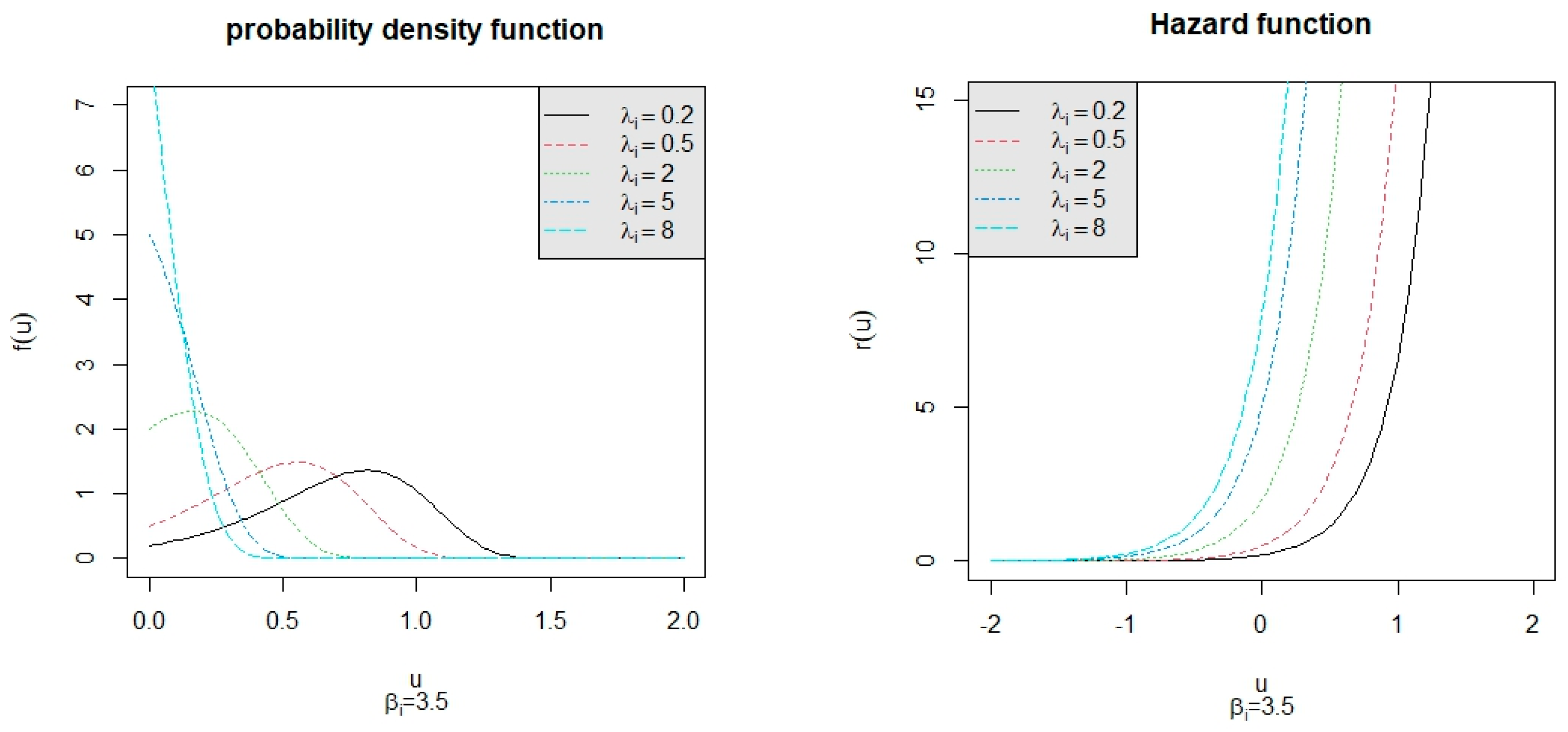
To explore the properties of Gompertz distribution, the p.d.f. and h.f. for ${\lambda }_i$ = 0.2, 0.5, 2, 5, 8 under ${\beta }_i$ = 2.5 are depicted in Figure 1. The p.d.f. and h.f. for ${\lambda }_i$ = 0.2, 0.5, 2, 5, 8 under ${\beta }_i$ = 3.5 are depicted in Figure 2. From the left panels of Figure 1 and Figure 2, we observe that the shape of the p.d.f. changes when $\mathrm{t}\mathrm{h}\mathrm{e} \mathrm{p}\mathrm{a}\mathrm{r}\mathrm{a}\mathrm{m}\mathrm{e}\mathrm{t}\mathrm{e}\mathrm{r} {\lambda }_i$ changes and the parameter ${\beta }_i$ only affects the degree of data dispersion. Additionally, the right panels of Figure 1 and Figure 2 show that the hazard rate increases exponentially as u increases. These properties make the Gompertz distribution well-suited for modeling aging-related processes where the likelihood of failure increases exponentially with time. Let us compare this model with the Weibull distribution. The Weibull distribution is versatile, supporting various hazard shapes, including increasing, decreasing, and constant rates. While the Weibull model is more versatile and widely used in reliability engineering, the Gompertz model offers unique advantages in scenarios where the failure rate aligns with biological or exponential growth patterns. Its simplicity and focus on exponential hazard rate growth make it a strong choice for aging-related life tests. Because the Gompertz distribution is an asymmetric probability distribution, this research pertains to the subject of asymmetric probability distributions and their applications in diverse fields. For the estimation for different censoring schemes for this distribution, refer to Srivastava [29].

Let $Y_i={\displaystyle \frac{1}{{\beta }_i}}\left(e^{{\beta }_i{U}_i}-1\right)$; then, we have the new random variable $Y_i$ following an exponential distribution with rate parameter ${\lambda }_i$ and the p.d.f. of ${ Y}_i$ is given by

$$f_{Y_i}\left(y\right)={\lambda }_i{e}^{-{\lambda }_{i}y}, y>0, {\lambda }_i>0.$$

(4)

The cumulative distribution function (c.d.f.) and the hazard function (h.f.) of $Y_i$ are defined as follows:

$$F_{Y_i}\left(y\right)=1-e^{-{\lambda }_{i}y}, y>0, {\lambda }_i>0,$$

(5)

$$r_{Y_i}\left(y\right)={\displaystyle \frac{f_{Y_i}\left(y\right)}{1-F_{Y_i}\left(y\right)}}={\lambda }_i.$$

(6)

To evaluate the larger-the-better lifetime performance, the lifetime performance index introduced by Montgomery [1] as follows is used in this study. Suppose that $L_{Ui}$ is the specified lower specification limit for $U_i$; then, $L_i={\displaystyle \frac{1}{{\beta }_i}}\left(e^{{\beta }_i{L}_{U_i}}-1\right)$ is the lower specification limit for ${ Y}_i$. We found that ${\mu }_i=E\left(Y_i\right)={\displaystyle \frac{1}{{\lambda }_i}} \mathrm{a}\mathrm{n}\mathrm{d} { \sigma }_i=\sqrt{Var\left(Y_i\right)}={\displaystyle \frac{1}{{\lambda }_i}}$ as the mean and the standard deviation of $Y_i$. Based on this information, the lifetime performance index for the production of the ith part, as stated by Montgomery [1], is defined as

$$C_{L_i}={\displaystyle \frac{{\mu }_i-L_i}{{ \sigma }_i}}={\displaystyle \frac{\frac{1}{{\lambda }_i}-L_i}{\frac{1}{{\lambda }_i}}}=1-{\lambda }_i{L}_i.$$

(7)

From the above equation, it is observed that this index $C_{L_i}$ increases as the hazard rate ${\lambda }_i$ decreases.

A product on the ith production line for producing ith part is considered to be conforming if the related lifetime surpasses $L_i$ so that the proportion of conforming products for the ith part is obtained as

$$P_{ri}=P\left(U_i\ge L_{Ui}\right)=e^{-{\lambda }_i{L}_i}=e^{C_{L_i}-1},-\infty <C_{L_i}<1.$$

(8)

$\mathrm{H}\mathrm{e}\mathrm{r}\mathrm{e}, P_{ri} \mathrm{i}\mathrm{s} \mathrm{t}\mathrm{h}\mathrm{e} \mathrm{s}\mathrm{o}-\mathrm{c}\mathrm{a}\mathrm{l}\mathrm{l}\mathrm{e}\mathrm{d} \mathrm{t}\mathrm{h}\mathrm{e} \mathrm{p}\mathrm{r}\mathrm{o}\mathrm{c}\mathrm{e}\mathrm{s}\mathrm{s} \mathrm{y}\mathrm{i}\mathrm{e}\mathrm{l}\mathrm{d} \mathrm{w}\mathrm{h}\mathrm{i}\mathrm{c}\mathrm{h} \mathrm{i}\mathrm{s} \mathrm{a}\mathrm{n} \mathrm{i}\mathrm{n}\mathrm{c}\mathrm{r}\mathrm{e}\mathrm{a}\mathrm{s}\mathrm{i}\mathrm{n}\mathrm{g} \mathrm{f}\mathrm{u}\mathrm{n}\mathrm{c}\mathrm{t}\mathrm{i}\mathrm{o}\mathrm{n} \mathrm{o}\mathrm{f} C_{L_i}.$

Suppose that the productions of d parts of products in d production lines are independent. We can find the overall process yield $P_r$ as

$$P_r=P\left(Y_i\ge L_i, i=1,2,\dots ,d\right)=e^{-{\sum }_{i=1}^d{\lambda }_i{L}_i}=e^{{\sum }_{i=1}^d{C}_{L_i}-d},-\infty <C_{L_i}<1.$$

(9)

The overall lifetime performance index C_T defined in the work by Wu and Chiang [24] is employed in this study and it satisfies the following equation:

$$P_r=\mathrm{e}\mathrm{x}\mathrm{p}\left\{C_T-1\right\},-\infty <C_T<1.$$

(10)

The index $C_T$ is designed to have a strictly increasing relationship with the overall process yield $P_r$. According to Equations (9) and (10), we yield the relationship between the overall lifetime performance index $C_T$ and the individual lifetime performance index $C_{L_i}$ as follows:

$$C_T=\left({\sum }_{i=1}^d{C}_{L_i}-d\right)+1={\sum }_{i=1}^d{C}_{L_i}-\left(d-1\right),-\infty <C_T<1.$$

(11)

To present a new overall lifetime performance index when we have d parts of products produced in d dependent production lines, the Bonferroni inequality stated in Lemma 1 is needed.

Lemma 1.

Let $A_1,A_2,\dots ,A_d$ be d events; then, ${P(A}_1\bigcap A_2\dots \bigcap A_d)\ge {\sum }_{i=1}^{d}P\left(A_i\right)-\left(d-1\right).$

Using Lemma 1, we can find the lower bound of the overall process yield as follows:

$$P_r=P\left(Y_i\ge L_i,\hspace{0.33em}i=1,\dots ,k\right)\ge {\sum }_{i=1}^d{e}^{-{\lambda }_i{L}_i}-\left(d-1\right)={\sum }_{i=1}^d{e}^{C_{Li}-1}-\left(d-1\right).$$

Set the lower bound of the overall process yield to be $P_{rl}$. Let the overall lifetime performance index $C_T$ satisfy

$$P_{rl}=\exp \left\{C_T-1\right\}={\sum }_{i=1}^d{e}^{C_{Li}-1}-\left(d-1\right),\hspace{0.33em}-\infty <C_T<1.$$

(12)

Observe that $C_T$ is an increasing function of P_rl. Solving Equation (12), we have the relationship between the overall lifetime performance index and individual lifetime performance index for each production line as follows:

$$C_T=\ln \left({\sum }_{i=1}^d{e}^{C_{Li}-1}-\left(d-1\right)\right)+1,\hspace{0.33em}-\infty <C_T<1.$$

(13)

A reasonable assumption in this context is that the capabilities of the production lines are equally important for quality engineers across all product parts. This rational configuration of equal individual lifetime performance indices is defined as follows: $C_{L_1}=C_{L_2}=\cdots =C_{L_d}=C_L$.

For the independence case, substituting this configuration into Equation (11), we obtain the relationship between $C_T$ and $C_L$ as

$$C_L={\displaystyle \frac{C_T+d-1}{d}},-\infty <C_T<1.$$

(14)

Suppose that the analyst desires the overall yield $P_r$ to exceed 0.9277; then, $C_T$ is found to be greater than 0.925 from Equation (10). From Equation (14), the corresponding values of $C_L$ are found to be 0.9625, 0.9750, 0.9812, 0.9850, 0.9875, 0.9893, 0.9906, 0.9917, 0.9925 for d = 2, 3, 4, 5, 6, 7, 8, 9, 10. Observe that the inequality $C_L$ > $C_T$ holds, when d > 1; that is, the equality $C_L=C_T$ holds, when d = 1.

For dependence case, ${\mathrm{u}\mathrm{n}\mathrm{d}\mathrm{e}\mathrm{r} \mathrm{t}\mathrm{h}\mathrm{e} \mathrm{a}\mathrm{s}\mathrm{s}\mathrm{u}\mathrm{m}\mathrm{p}\mathrm{t}\mathrm{i}\mathrm{o}\mathrm{n} \mathrm{o}\mathrm{f} C}_{L_1}=C_{L_2}=\cdots =C_{L_d}=C_L$, we obtain the relationship between $C_T$ and $C_L$ as

$$C_L=\ln \left((\exp \left\{C_T-1\right\}+(d-1\left)\right)/d\right)+1,\hspace{0.33em}-\infty <C_T<1.$$

(15)

Suppose that the analyst desires the lower bound of the overall process yield P_rl to be 0.9277, the value of $C_T$ is found to be 0.925 from Equation (12). The corresponding values of $C_L$ are found to be 0.9632, 0.9756, 0.9818, 0.9854, 0.9879, 0.9896, 0.9909, 0.9919, 0.9927 for d = 2, 3, 4, 5, 6, 7, 8, 9, 10 from Equation (15). Observe that the values of $C_L$ for the dependent case are slightly higher than those for the independent case under the same value of $C_T$ and $P_{rl}=P_r$.

2.2. The Maximum Likelihood Estimators and Their Asymptotic Distributions for the Lifetime Performance Indices

The progressive type I interval-censoring is depicted as follows: For the ith production line for producing the ith part, let n products undergo a life test with m inspection intervals with the predetermined inspection time points (t₁, …, t_m), where t_m is the termination time of this experiment. Once the number of failure units X_ij is observed at the time point of t_j, R_ij products are randomly removed under the removal probability p_j, j = 1, …, m. The number of failure units X_ij follows a binomial distribution denoted by bin($n-{\sum }_{l=1}^{j-1}{X}_{il}-{\sum }_{l=1}^{j-1}{R}_{il}$, q_ij), where $q_{ij}={\displaystyle \frac{F_{U_i}\left(t_j\right)-F_{U_i}\left(t_{j-1}\right)}{1-F_{U_i}\left(t_{j-1}\right)}}$ and $F_{U_i}\left(x\right)$ denotes the cdf for the lifetime variable of the ith part. The number of removal units R_ij follows a binomial distribution denoted by bin($n-{\sum }_{l=1}^j{X}_{il}-{\sum }_{l=1}^{j-1}{R}_{il}$, p_j), where p_j is the pre-assigned removal probability, j = 1, …, m. Once the experiment is completed, the progressive type I interval-censored sample $\left(X_{i1},\dots ,X_{im}\right)$ is collected under the censoring scheme of $\left(R_{i1},\cdots ,R_{im}\right)$ for the ith production line.

Based on the progressive type I interval-censored sample $\left(X_{i1},\dots ,X_{im}\right)$ for the lifetimes of the ith part of products at the time points $\mathrm{o}\mathrm{f}\left(t_1,\cdots ,t_m\right)$ under the progressive censoring scheme of $\left(R_{i1},\cdots ,R_{im}\right)$, we make inferences on the overall lifetime performance index and each individual lifetime performance index. The likelihood function of the censored sample $\left(X_{i1},\dots ,X_{im}\right)$ is

$$\begin{gathered} L\left({\lambda }_i\right)\propto {\prod }_{j=1}^m{\left(F_{U_i}\left(t_j\right)-F_{U_i}\left(t_{j-1}\right)\right)}^{X_{ij}}{\left(1-F_{U_i}\left(t_j\right)\right)}^{R_{ij}} \\ \propto {\prod }_{j=1}^m{\left(1-e^{-{\lambda }_i\left(y_{ij}-y_{i,j-1}\right)}\right)}^{X_{ij}}\left(e^{-{\lambda }_i\left({R_{ij}y}_{ij}+X_{ij}{y}_{i,j-1}\right)}\right), \end{gathered}$$

(16)

where $y_{ij}={\displaystyle \frac{1}{{\beta }_i}}\left(e^{{\beta }_i{t}_j}-1\right).$ We obtain the log-likelihood function as

$$\mathrm{l}\mathrm{n}L\left({\lambda }_i\right)={\sum }_{j=1}^m{X}_{ij} \mathrm{l}\mathrm{n}\left(1-w_{ij}\right)-{\lambda }_i{\sum }_{j=1}^m\left(R_{ij}{y}_{ij}+X_{ij}{y}_{i,j-1}\right),$$

(17)

where $w_{ij}=e^{-{\lambda }_i\left(y_{ij}-y_{i,j-1}\right)}$.

By taking the derivative to Equation (17) with respect to the parameter ${\lambda }_i$ and equating it to zero, we yield the log-likelihood equation as

$${\displaystyle \frac{d}{d{\lambda }_i}}\mathrm{l}\mathrm{n}L\left({\lambda }_i\right)=-{\sum }_{j=1}^m{X}_{ij}\left(\mathrm{l}\mathrm{n}{w}_{ij}\right)w_{ij}/\left({\lambda }_i\right(1-w_{ij}\left)\right)-{\sum }_{j=1}^m\left(R_{ij}{y}_{ij}+X_{ij}{y}_{i,j-1}\right)=0,$$

(18)

The solution of the above derivative of the log-likelihood equation is the maximum likelihood estimator for the parameter ${\lambda }_i$, denoted by ${\widehat{\lambda }}_i$. To show that this solution is indeed attaining the maximum, we take the second derivative of the log-likelihood function as follows:

$${\displaystyle \frac{d^2}{d{{\lambda }_i}^2}}\mathrm{l}\mathrm{n}L\left({\lambda }_i\right)=-{\sum }_{j=1}^m{X}_{ij}{\left(\mathrm{l}\mathrm{n}{w}_{ij}\right)}^2{w}_{ij}/{\left({\lambda }_i\right(1-w_{ij}\left)\right)}^2.$$

(19)

Since it is negative, the solution for the log-likelihood equation as ${\widehat{\lambda }}_i$ should be the maximum likelihood estimator. The other approach to find the maximum likelihood estimator is using the Expectation–Maximization (EM) algorithm for incomplete data. Each iteration of the EM algorithm consists of two steps including the E-step (expectation-step) and the M-step (maximization step). Let $U_{ijl},l=1,\dots ,X_{ij},j=1,\dots ,m$ be the failure times in the jth time interval $[t_{j-1},t_j)$ and ${\tilde{U}}_{ijl},l=1,\dots ,R_{ij},j=1,\dots ,m$ be the failure times of removing units in time interval $[t_j,\infty ),j=1,\dots ,m$. The log-likelihood function for the complete sample is

$$\begin{gathered} \mathrm{l}\mathrm{n}L\left({\lambda }_i\right)=-{\sum }_{j=1}^{\begin{array}{c} \\ m \end{array}}\left({\sum }_{l=1}^{\begin{array}{c} \\ X_{ij} \end{array}}{u}_{ijl}+{\sum }_{l=1}^{\begin{array}{c} \\ R_{ij} \end{array}}{\tilde{u}}_{ijl}\right)/{\lambda }_i-\ln {\lambda }_i{\sum }_{j=1}^m\left(X_{ijl}+R_{ijl}\right) \\ =-{\sum }_{j=1}^{\begin{array}{c} \\ m \end{array}}\left({\sum }_{l=1}^{\begin{array}{c} \\ X_{ij} \end{array}}{u}_{ijl}+{\sum }_{l=1}^{\begin{array}{c} \\ R_{ij} \end{array}}{\tilde{u}}_{ijl}\right)/{\lambda }_i-n\ln {\lambda }_i. \end{gathered}$$

(20)

Taking derivative with respect to parameter ${\lambda }_i$ and equating to zero, we have the log-likelihood equation

$${\sum }_{j=1}^{\begin{array}{c} \\ m \end{array}}\left({\sum }_{l=1}^{\begin{array}{c} \\ X_{ij} \end{array}}{u}_{ijl}+{\sum }_{l=1}^{\begin{array}{c} \\ R_{ij} \end{array}}{\tilde{u}}_{ijl}\right)/{\lambda }_i^2-n/{\lambda }_i=0.$$

To solve the above equation, we have the maximum likelihood estimator of ${\lambda }_i$ given by

$${\widehat{\lambda }}_i={\sum }_{j=1}^{\begin{array}{c} \\ m \end{array}}\left({\sum }_{l=1}^{\begin{array}{c} \\ X_{ij} \end{array}}{u}_{ijl}+{\sum }_{l=1}^{\begin{array}{c} \\ R_{ij} \end{array}}{\tilde{u}}_{ijl}\right)/n.$$

(21)

The expected failure times of $U_{ijl},l=1,\dots ,X_{ij},j=1,\dots ,m$ and ${\tilde{U}}_{ijl},l=1,\dots ,R_{ij},j=1,\dots ,m$ are given by

$$\begin{gathered} e_{{\lambda }_i,ijl}=E(U_{ijl}|u_{ijl}\in [t_{j-1},t_j))={\int }_{t_{j-1}}^{t_j}{u}_{ijl}{e}^{-{\displaystyle \frac{u_{ijl}}{{\lambda }_i}}}d{u}_{ijl}/{\lambda }_i(e^{-{\displaystyle \frac{t_{j-1}}{{\lambda }_i}}}-e^{-{\displaystyle \frac{t_j}{{\lambda }_i}}}) \\ =t_{j-1}{e}^{-{\displaystyle \frac{t_{j-1}}{{\lambda }_i}}}-t_j{e}^{-{\displaystyle \frac{t_j}{{\lambda }_i}}}-{\lambda }_i{e}^{-{\displaystyle \frac{t_j}{{\lambda }_i}}}+{\lambda }_i{e}^{-{\displaystyle \frac{t_{j-1}}{{\lambda }_i}}}/(e^{-{\displaystyle \frac{t_{j-1}}{{\lambda }_i}}}-e^{-{\displaystyle \frac{t_j}{{\lambda }_i}}}). \end{gathered}$$

(22)

$${\tilde{e}}_{\lambda ,ijl}=E({\tilde{U}}_{ijl}|{\tilde{u}}_{ijl}\in [t_j,\infty ))={\int }_{t_j}^{\infty }{\tilde{u}}_{ijl}{e}^{-{\displaystyle \frac{{\tilde{u}}_{ijl}}{{\lambda }_i}}}d{\tilde{u}}_{ijl}/{\lambda }_i{e}^{-{\displaystyle \frac{t_j}{{\lambda }_i}}}=(t_j{e}^{-{\displaystyle \frac{t_{j-1}}{{\lambda }_i}}}+{\lambda }_i{e}^{-{\displaystyle \frac{t_j}{{\lambda }_i}}})/e^{-{\displaystyle \frac{t_j}{{\lambda }_i}}}.$$

(23)

The iterative process for obtaining the maximum likelihood estimator of ${\lambda }_i$ with the EM algorithm is in Algorithm 1.

Algorithm 1: The iterative process for EM algorithm

Step 1: Set the initial value of ${\lambda }_i$ to be ${\widehat{\lambda }}_i^{\left(0\right)}$, k = 0. Step 2: For the E-step: Calculate the expected failure times of $e_{{\lambda }_i,ijl}$ and ${\tilde{e}}_{\lambda ,ijl}$. Replace $u_{ijl}$ and ${\tilde{u}}_{ijl}$ by $e_{{\widehat{\lambda }}_i^{\left(k\right)},ijl}$ and ${\tilde{e}}_{{\widehat{\lambda }}_i^{\left(k\right)},ijl}$ in the log-likelihood function given in Equation (20) to have a new log-likelihood function. Step 3: For the M-step: The log-likelihood equation is ${\sum }_{j=1}^{\begin{array}{c} \\ m \end{array}}\left({\sum }_{l=1}^{\begin{array}{c} \\ X_{ij} \end{array}}{e}_{{\widehat{\lambda }}_i^{\left(k\right)},ijl }+{\sum }_{l=1}^{\begin{array}{c} \\ R_{ij} \end{array}}{\tilde{e}}_{{\widehat{\lambda }}_i^{\left(k\right)},ijl}\right)/{\lambda }_i^2-n/{\lambda }_i=0$. Solve this equation to have the next value of ${\lambda }_i$ given by ${\widehat{\lambda }}^{(k+1)}={\sum }_{j=1}^{\begin{array}{c} \\ m \end{array}}\left({\sum }_{l=1}^{\begin{array}{c} \\ X_{ij} \end{array}}{e}_{{\widehat{\lambda }}_i^{\left(k\right)},ijl }+{\sum }_{l=1}^{\begin{array}{c} \\ R_{ij} \end{array}}{\tilde{e}}_{{\widehat{\lambda }}_i^{\left(k\right)},ijl}\right)/n$. Step 4: Set k = k + 1 and repeat steps 2–4 until ${\widehat{\lambda }}_i^{\left(0\right)},\dots ,{\widehat{\lambda }}_i^{(k+1)}$ converges. Then, ${\widehat{\lambda }}_i^{(k+1)}$ is the approximate maximum likelihood estimator of ${\lambda }_i$.

Referring to Casella and Berger [29], we can state that the asymptotic distribution of the maximum likelihood estimator ${\widehat{\lambda }}_i$ is the normal distribution with the variance given by $\mathrm{t}\mathrm{h}\mathrm{e} \mathrm{i}\mathrm{n}\mathrm{v}\mathrm{e}\mathrm{r}\mathrm{s}\mathrm{e} \mathrm{o}\mathrm{f} \mathrm{t}\mathrm{h}\mathrm{e} \mathrm{F}\mathrm{i}\mathrm{s}\mathrm{h}\mathrm{e}\mathrm{r}’\mathrm{s} \mathrm{i}\mathrm{n}\mathrm{f}\mathrm{o}\mathrm{r}\mathrm{m}\mathrm{a}\mathrm{t}\mathrm{i}\mathrm{o}\mathrm{n} \mathrm{n}\mathrm{u}\mathrm{m}\mathrm{b}\mathrm{e}\mathrm{r} I\left({\lambda }_i\right),$ where the Fisher’s information number is defined as $I\left({\lambda }_i\right)=-E\left[{\displaystyle \frac{d^2\mathrm{l}\mathrm{n}L\left({\lambda }_i\right)}{d{\lambda }_i^2}}\right]$.

For the progressive type I interval-censoring, we assume that the number of failures $X_{ij}$ is following a binomial distribution denoted by

$$X_{ij}\left|X_{i,j-1}\right.,\dots ,X_{i1},R_{i,j-1},\cdots ,R_{i1}~\mathrm{B}\mathrm{i}\mathrm{n}\mathrm{o}\mathrm{m}\mathrm{i}\mathrm{a}\mathrm{l}\left(n-{\sum }_{l=1}^{j-1}{X}_{il}-{\sum }_{l=1}^{j-1}{R}_{il},q_{ij}\right),$$

(24)

where $q_{ij}={\displaystyle \frac{F\left(t_j\right)-F\left(t_{j-1}\right)}{1-F\left(t_{j-1}\right)}}=1-\mathrm{e}\mathrm{x}\mathrm{p}\left(-{\displaystyle \frac{{\lambda }_i}{{\beta }_i}}\left(e^{{\beta }_i{t}_j}-e^{{\beta }_i{t}_{j-1}}\right)\right),j=1,\dots ,m,i=1,\dots ,d.$ Additionally, we assume that the number of progressive censorings at the jth observation time point is coming from a binomial distribution denoted by

$$R_{ij}\left|R_{i,j-1}\right.,\dots ,R_{i1},X_{i,j},\cdots ,X_{i1}~\mathrm{B}\mathrm{i}\mathrm{n}\mathrm{o}\mathrm{m}\mathrm{i}\mathrm{a}\mathrm{l}\left(n-{\sum }_{l=1}^j{X}_{il}-{\sum }_{l=1}^{j-1}{R}_{il},p_j\right),$$

(25)

where $p_j$ is the removal probability for the number of removals $R_{ij}$ at the jth inspection time point $t_j$.

Based on the conditional probabilities given in Equations (24) and (25), we yield the expected values for $X_{ij} \mathrm{a}\mathrm{n}\mathrm{d} R_{ij}$ as

$$E\left(X_{ij}\right)=n{q}_{ij}{\prod }_{l=1}^{j-1}(1-q_{il})(1-p_l),j=1,\dots ,m.$$

(26)

$$E\left(R_{ij}\right)=n{p}_j\left(1-q_{ij}\right){\prod }_{l=1}^{j-1}(1-q_{il})(1-p_l), j=1,\dots ,m.$$

(27)

Using Equations (22) and (23), we yield Fisher’s information number as

$$I\left({\lambda }_i\right)={\displaystyle \frac{n}{{{\beta }_i}^2}}{\sum }_{j=1}^m{\left(e^{{\beta }_i{t}_j}-e^{{\beta }_i{t}_{j-1}}\right)}^2{\prod }_{l=1}^{j-1}(1-q_{il})(1-p_l)/q_{ij}.$$

(28)

The asymptotic normal distribution of ${\widehat{\lambda }}_i$ is denoted as

$${\widehat{\lambda }}_i\underset{n\to \mathrm{\infty }}{\stackrel{d}{\to }}\mathrm{N}({\lambda }_i,I^{-1}\left({\lambda }_i\right)).$$

Applying the property of invariance for the maximum likelihood estimator, we can find the maximum likelihood estimator for the lifetime performance index $C_{L_i}$ as

$${\widehat{C}}_{L_i}=1-{\widehat{\lambda }}_i{L}_i.$$

(29)

For this purpose, the Delta method is applied, which is a statistical approach used to approximate the distribution of a function of an estimator, especially when the estimator has a known asymptotic distribution, commonly a normal distribution. Applying the Delta method in Casella and Berger [29], we yield

$${\widehat{C}}_{L_i} \begin{array}{c}d\\ \overrightarrow{n\to \infty }\end{array} N\left(C_{L_i},{L_i}^{2}V\left({\widehat{\lambda }}_i\right)\right),$$

(30)

 where $V\left({\widehat{\lambda }}_i\right)=I^{-1}\left({\lambda }_i\right).$

Referring to the overall lifetime performance index $C_T$, we can find the maximum likelihood estimator for $C_T$ as

$${\widehat{C}}_T={\sum }_{i=1}^d{\widehat{C}}_{L_i}-\left(d-1\right),-\infty <C_T<1.$$

(31)

Due to d independent production lines, the asymptotic variance of ${\widehat{C}}_T$ is $\mathrm{o}\mathrm{b}\mathrm{t}\mathrm{a}\mathrm{i}\mathrm{n}\mathrm{e}\mathrm{d}\mathrm{a}\mathrm{s} V\left({\widehat{C}}_T\right)={\sum }_{i=1}^{d}V\left({\widehat{C}}_{L_i}\right)$ and its estimator is ${\sum }_{i=1}^d\widehat{V}\left({\widehat{C}}_{L_i}\right)$. Additionally, we obtain the asymptotic distribution for ${\widehat{C}}_T$ as

$${\widehat{C}}_T \begin{array}{c}d\\ \overrightarrow{n\to \infty }\end{array} N\left(C_T,{\sum }_{i=1}^d\widehat{V}\left({\widehat{C}}_{L_i}\right)\right),$$

(32)

where $V\left({\widehat{C}}_T\right)={\displaystyle \sum _{i=1}^d}V\left({\widehat{C}}_{L_i}\right) \mathrm{a}\mathrm{n}\mathrm{d} V\left({\widehat{C}}_{L_i}\right)={L_i}^{2}V\left({\widehat{\lambda }}_i\right).$

For the dependent case, we can find the maximum likelihood estimator for $C_T$ as

$${\widehat{C}}_T=\ln \left({\sum }_{i=1}^d{e}^{{\widehat{C}}_{L_i}-1}-\left(d-1\right)\right)+1.$$

(33)

We can also obtain the asymptotic distribution for ${\widehat{C}}_T$ as

$${\widehat{C}}_T \begin{array}{c}d\\ \overrightarrow{n\to \infty }\end{array} N\left(C_T, V\left({\widehat{C}}_T\right)\right),$$

(34)

$\mathrm{w}\mathrm{h}\mathrm{e}\mathrm{r}\mathrm{e} V\left({\widehat{C}}_T\right)=Var\left(\ln \left({\sum }_{i=1}^d{e}^{{\widehat{C}}_{L_i}-1}-\left(d-1\right)\right)+1\right).$

3. The Testing Algorithm Procedure Related to the Overall Lifetime Performance Index

In Section 3.1, the testing procedure to determine whether the overall lifetime performance index reaches the target level for this index and the relevant power analysis is provided. Section 3.2 analyzes the test power and a simulation study is conducted for the test powers. Section 3.3 provides a numerical example to illustrate the testing procedure related to the overall lifetime performance index.

3.1. The Testing Procedure for the Overall Lifetime Performance Index

Firstly, let us assume that the manufacturer sets a target level $c_0$ for the overall lifetime performance $C_T$ for products with d parts produced in d independent production lines. To test whether the overall lifetime performance reaches the target level $c_0$, the null and alternative hythesis are setup as $H_0:C_T\le c_0$ v.s. $H_1:C_T>c_0.$ For the independent case, using the maximum likelihood estimator ${\widehat{C}}_T$ as the test statistics, the critical value $C_{T0}$ for the level α test is determined as follows: Set the power function P(${\widehat{C}}_T>C_{T0}|C_T=c_0$) = α; then, the critical value $C_{T0}$ is determined as $C_{T0}=c_0+Z_{\mathsf{\alpha }}\sqrt{V\left({\widehat{C}}_T\right)}, \mathrm{w}\mathrm{h}\mathrm{e}\mathrm{r}\mathrm{e} V\left({\widehat{C}}_T\right) \mathrm{i}\mathrm{s} \mathrm{d}\mathrm{e}\mathrm{f}\mathrm{i}\mathrm{n}\mathrm{e}\mathrm{d} \mathrm{i}\mathrm{n} \mathrm{E}\mathrm{q}\mathrm{u}\mathrm{a}\mathrm{t}\mathrm{i}\mathrm{o}\mathrm{n} (25)$. If ${\widehat{C}}_T>C_{T0}$, we can infer that the overall lifetime performance reaches the target level. Furthermore, we also want to assess the performance of each production line as follows: Based on this target value of $c_0,$ the appropriate target value of $c_0^{*}={\displaystyle \frac{c_0+d-1}{d}}$ for the individual lifetime performance index $C_L$ can be found in the following table.

For instance, for d = 3, suppose the analyst wants the overall yield $P_r$ to surpass 0.8607. In this case, $c_0$ must exceed 0.85 and the target value for the individual lifetime performance index $c_0^{*}$ is determined as 0.95 from

Table 1. The corresponding target values of $c_0^{*}$ for a given value of $P_r$ and the target value $c_0.$

${\mathit{c}}_0^{\mathit{*}}$
Pr	c0\d	2	3	4	5	6	7
0.6873	0.6250	0.8125	0.8750	0.9063	0.9250	0.9375	0.9464
0.7047	0.6500	0.8250	0.8833	0.9125	0.9300	0.9417	0.9500
0.7225	0.6750	0.8375	0.8917	0.9188	0.9350	0.9458	0.9536
0.7408	0.7000	0.8500	0.9000	0.9250	0.9400	0.9500	0.9571
0.7596	0.7250	0.8625	0.9083	0.9313	0.9450	0.9542	0.9607
0.7788	0.7500	0.8750	0.9167	0.9375	0.9500	0.9583	0.9643
0.7985	0.7750	0.8875	0.9250	0.9438	0.9550	0.9625	0.9679
0.8187	0.8000	0.9000	0.9333	0.9500	0.9600	0.9667	0.9714
0.8395	0.8250	0.9125	0.9417	0.9563	0.9650	0.9708	0.9750
0.8607	0.8500	0.9250	0.9500	0.9625	0.9700	0.9750	0.9786
0.8825	0.8750	0.9375	0.9583	0.9688	0.9750	0.9792	0.9821
0.9048	0.9000	0.9500	0.9667	0.9750	0.9800	0.9833	0.9857
0.9277	0.9250	0.9625	0.9750	0.9813	0.9850	0.9875	0.9893
0.9512	0.9500	0.9750	0.9833	0.9875	0.9900	0.9917	0.9929
0.9753	0.9750	0.9875	0.9917	0.9938	0.9950	0.9958	0.9964
1.0000	1.0000	1.0000	1.0000	1.0000	1.0000	1.0000	1.0000

.

For the dependent case, based on this target value of $c_0,$ the appropriate target value of $c_0^{*}=\ln \left((\exp \left\{c_0-1\right\}+(d-1\left)\right)/d\right)+1$ for the individual lifetime performance index $C_L$ can be found in the following table.

Then, we can establish a set of null hypothesis and alternative hypothesis as follows:

$$H_0:C_{L_i}\le c_0^{*},\mathrm{for} \mathrm{some} i \mathrm{v}.\mathrm{s}. H_1:C_{L_i}>c_0^{*}, i=1,\dots ,d.$$

This hypothesis test is known as the Intersection–Union Test (IUT) in the work of Casella and Berger [30].

Referring to the ith test of $H_{0i}:C_{L_i}\le c_0^{* } \mathrm{v}\mathrm{s}. H_{1i}:C_{L_i}>c_0^{*}$, the maximum likelihood estimator of the individual lifetime performance index as ${\widehat{C}}_{L_i}=1-{\widehat{\lambda }}_i{L}_i$ is used as the test statistics, I = 1, …, d. For the independent case, the critical value $C_{L_i}^0$ for the ith test is $C_{L_i}^0=1-L_i\left(Z_{{\alpha }^{\prime }}\sqrt{I^{-1}\left({\lambda }_{i0}\right)}+{\lambda }_{i0}\right)$, where ${\lambda }_{i0}={\displaystyle \frac{1-c_0^{*}}{L_i}}$, α′ = α^1/d and $I_i\left({\lambda }_{i0}\right)$ is defined in Equation (24) by replacing ${\lambda }_i$ by ${\lambda }_{i0},i=1,\cdots ,d$.

We are going to find the critical value denoted by $C_{L_{iw}}^0$ for the dependent case with respect to the ith test. For the dependent case, the lower bound of the power function at $C_T$ = c₀ is obtained as follows by using Lemma 1:

$$\begin{array}{c}h\left(c_1\right)=P\left({\widehat{C}}_{L_i}>C_{L_{iw}}^0|c_0^{*}=1-{\lambda }_{i0}{L}_{i }, i=1,\dots ,d\right)\hfill \\ =P\left(1-{\widehat{\lambda }}_i{L}_i>C_{L_{iw}}^0\left|{\lambda }_{i0}={\displaystyle \frac{1-c_0^{*}}{L_i}}\right.,i=1,\dots ,d\right)\hfill \\ =P\left({\widehat{\lambda }}_i<{\displaystyle \frac{1-C_{L_{iw}}^0}{L_i}}\left|{\lambda }_{i0}={\displaystyle \frac{1-c_0^{*}}{L_i}},\right.i=1,\dots ,d\right)\hfill \\ =P\left(Z<({\displaystyle \frac{1-C_{L_{iw}}^0}{L_i}}-{\lambda }_{i0})/\sqrt{I^{-1}\left({\lambda }_{i0}\right)}\left|{\lambda }_{i0}={\displaystyle \frac{1-c_0^{*}}{L_i}},\right.i=1,\dots ,d\right)\hfill \\ \ge {\sum }_{i=1}^{d}P\left(Z<({\displaystyle \frac{1-C_{L_{iw}}^0}{L_i}}-{\lambda }_{i0})/\sqrt{I^{-1}\left({\lambda }_{i0}\right)}| {\lambda }_{i0}={\displaystyle \frac{1-c_0^{*}}{L_i}}\right)-\left(d-1\right)\hfill \\ =d\Phi \left(({\displaystyle \frac{1-C_{L_{iw}}^0}{L_i}}-{\lambda }_{i0})/\sqrt{I^{-1}\left({\lambda }_{i0}\right)}| {\lambda }_0={\displaystyle \frac{1-c_0^{*}}{L}}\right)-(d-1).\hfill \end{array}$$

The above inequality holds by using Lemma 1.

Set $\Phi \left(({\displaystyle \frac{1-C_{L_{iw}}^0}{L_i}}-{\lambda }_{i0})/\sqrt{I^{-1}\left({\lambda }_{i0}\right)}| {\lambda }_0={\displaystyle \frac{1-c_0^{*}}{L}}\right)={\alpha }^{″}$, where ${\alpha }^{″}={\displaystyle \frac{\alpha +d-1}{d}}$. Then, the probability of type I error attains α. Solving this equation, we can obtain the critical value $C_{L_{iw}}^0=1-L_i\left(Z_{1-{\alpha }^{″}}\sqrt{I^{-1}\left({\lambda }_{i0}\right)}+{\lambda }_{i0}\right)$ for level α test. We propose a testing procedure for testing $H_0:C_T\le c_0$ v.s. $H_1:C_T>c_0$ in the following five steps:

• Step 1: For the given specified lower limits L_i, collect the progressive type I interval-censored samples $X_{i1},\dots ,X_{im}$ at the inspection times of $t_1,\dots ,t_m$ under the censoring schemes of $R_{i1},\dots ,R_{im}$ from the Gompertz distribution, I = 1, …, d.
• Step 2: From Table 1 or

  Table 2. The corresponding target values of $c_0^{*}$ for a given value of $P_{rl}$ and the target value $c_0$.

  ${\mathit{c}}_0^{\mathit{*}}$
  Prl	c0\d	2	3	4	5	6	7
  0.6873	0.6250	0.8300	0.8899	0.9186	0.9354	0.9465	0.9543
  0.7047	0.6500	0.8402	0.8964	0.9233	0.9391	0.9495	0.9569
  0.7225	0.6750	0.8506	0.9029	0.9281	0.9429	0.9527	0.9596
  0.7408	0.7000	0.8612	0.9096	0.9330	0.9468	0.9558	0.9623
  0.7596	0.7250	0.8719	0.9165	0.9380	0.9507	0.9591	0.9650
  0.7788	0.7500	0.8828	0.9234	0.9431	0.9548	0.9624	0.9679
  0.7985	0.7750	0.8938	0.9305	0.9483	0.9589	0.9658	0.9708
  0.8187	0.8000	0.9050	0.9377	0.9536	0.9631	0.9693	0.9738
  0.8395	0.8250	0.9163	0.9450	0.9590	0.9674	0.9729	0.9768
  0.8607	0.8500	0.9278	0.9525	0.9646	0.9717	0.9765	0.9799
  0.8825	0.8750	0.9395	0.9600	0.9702	0.9762	0.9802	0.9831
  0.9048	0.9000	0.9512	0.9678	0.9759	0.9808	0.9840	0.9863
  0.9277	0.9250	0.9632	0.9756	0.9818	0.9854	0.9879	0.9896
  0.9512	0.9500	0.9753	0.9836	0.9877	0.9902	0.9918	0.9930
  0.9753	0.9750	0.9876	0.9917	0.9938	0.9950	0.9959	0.9965
  1.0000	1.0000	1.0000	1.0000	1.0000	1.0000	1.0000	1.0000

  , for a desired overall process yield P_r, find the appropriate value of c₀ as the target value for C_T. Then, find the appropriate value of $c_0^{*}$ as the target value for C_L from Table 1 for the independent case and from Table 2 for the dependent case. Based on these target values, we can establish the testing hypothesis $H_0:C_{L_i}\le c_0^{*}$ for some i.s. $H_1:C_{L_i}>c_0^{*},i=1,\cdots ,d$.
• Step 3: Firstly, find the maximum likelihood estimators ${\widehat{\lambda }}_i,i=1,\cdots ,d,$ for d parts. Then, we can calculate the values of the test statistic ${\widehat{C}}_{L_i},i=1,\cdots ,d$.
• Step 4: For the given significance level α, find the critical values of $C_{L_i}^0=1-L_i\left(Z_{{\alpha }^{\prime }}\sqrt{I^{-1}\left({\lambda }_{i0}\right)}+{\lambda }_{i0}\right) \mathrm{f}\mathrm{o}\mathrm{r} \mathrm{t}\mathrm{h}\mathrm{e} \mathrm{i}\mathrm{n}\mathrm{d}\mathrm{e}\mathrm{p}\mathrm{e}\mathrm{n}\mathrm{d}\mathrm{e}\mathrm{n}\mathrm{t} \mathrm{c}\mathrm{a}\mathrm{s}\mathrm{e} \mathrm{a}\mathrm{n}\mathrm{d} C_{L_{iw}}^0=1-L_i\left(Z_{1-{\alpha }^{″}}\sqrt{I^{-1}\left({\lambda }_{i0}\right)}+{\lambda }_{i0}\right)$ for the dependent case, where ${\lambda }_{i0}={\displaystyle \frac{1-c_0^{\mathrm{*}}}{L_i}}$, α′ = α^1/d, ${\alpha }^{″}={\displaystyle \frac{\alpha +d-1}{d}}$ and $I_i\left({\lambda }_{i0}\right)$ is defined in Equation (24) by replacing ${\lambda }_i$ by ${\lambda }_{i0},i=1,\cdots ,d$.
• Step 5: For testing $H_0:C_{L_i}\le c_0^{*} \mathrm{f}\mathrm{o}\mathrm{r} \mathrm{s}\mathrm{o}\mathrm{m}\mathrm{e} i$ v.s. $H_1:C_{L_i}>c_0^{*},i=1,\cdots ,d,$ evaluate ${\widehat{C}}_{L_i}$ in comparison to $C_{L_i}^0,i=1,\cdots ,d$ for the independent case and in comparison to $C_{L_{iw}}^0$ for the dependent case. For the independent case, if ${\widehat{C}}_{L_i} \mathrm{i}\mathrm{s} \mathrm{g}\mathrm{r}\mathrm{e}\mathrm{a}\mathrm{t}\mathrm{e}\mathrm{r} \mathrm{t}\mathrm{h}\mathrm{a}\mathrm{n} C_{L_i}^0$ for all i, we can infer that all individual lifetime performance indices exceed the target level $c_0^{*}.$ Likewise, for the dependent case, if ${\widehat{C}}_{L_i} \mathrm{i}\mathrm{s} \mathrm{g}\mathrm{r}\mathrm{e}\mathrm{a}\mathrm{t}\mathrm{e}\mathrm{r} \mathrm{t}\mathrm{h}\mathrm{a}\mathrm{n} C_{L_{iw}}^0$ for all i, we can infer that all individual lifetime performance indices exceed the target level $c_0^{*}$.

3.2. Power Analysis and Simulation Study

In this section, we evaluate the test power function $h\left(c_1\right)$ for the IUT test for the independent case at the point of $C_T=d{C}_L-\left(d-1\right)=c_1>c_0$ or $C_L={\displaystyle \frac{c_1+d-1}{d}}=c_1^{*}$ in the alternative hypothesis of $H_1:C_{L_i}>c_0^{*},\mathrm{w}\mathrm{h}\mathrm{e}\mathrm{r}\mathrm{e} c_1^{*}>c_0^{*}.$ At this point $c_1^{*}$ in the alternative hypothesis, we yield the test power function as

$$\begin{array}{c}h\left(c_1\right)=P\left({\widehat{C}}_{L_i}>C_{L_i}^0|c_1^{*}=1-{\theta }_{i1}{L}_{i }, i=1,\dots ,d\right)\hfill \\ =P\left(1-{\widehat{\lambda }}_i{L}_i>1-L_i\left(Z_{{\alpha }^{\prime }}\sqrt{I^{-1}\left({\lambda }_{i0}\right)}+{\lambda }_{i0}\right)\left|{\lambda }_{i0}={\displaystyle \frac{1-c_0^{*}}{L_i}},{\lambda }_{i1}={\displaystyle \frac{1-c_1^{*}}{L_i}}\right.,i=1,\dots ,d\right)\hfill \\ =P\left({\widehat{\lambda }}_i<{\lambda }_{i0}+Z_{{\alpha }^{\prime }}\sqrt{I^{-1}\left({\lambda }_{i0}\right)},i=1,\cdots ,d|{\lambda }_{i1}={\displaystyle \frac{1-c_1^{*}}{L_i}},{\lambda }_{i0}={\displaystyle \frac{1-c_0^{*}}{L_i}},i=1,\cdots ,d\right)\hfill \\ ={\displaystyle \prod _{i=1}^d}P\left({\displaystyle \frac{{\widehat{\lambda }}_i{-\lambda }_{i1}}{\sqrt{I^{-1}\left({\lambda }_{i1}\right)}}}<{\displaystyle \frac{{\lambda }_{i0}{-\lambda }_{i1}+Z_{{\alpha }^{\prime }}\sqrt{I^{-1}\left({\lambda }_{i0}\right)}}{\sqrt{I^{-1}\left({\lambda }_{i1}\right)}}}| {\lambda }_{i1}={\displaystyle \frac{1-c_1^{*}}{L_i}},{\lambda }_{i0}={\displaystyle \frac{1-c_0^{*}}{L_i}}\right)\hfill \\ ={\prod }_{i=1}^d\left(\Phi \left({\displaystyle \frac{{\lambda }_{i0}{-\lambda }_{i1}+Z_{{\alpha }^{\prime }}\sqrt{I^{-1}\left({\lambda }_{i0}\right)}}{\sqrt{I^{-1}\left({\lambda }_{i1}\right)}}}| {\lambda }_{i1}={\displaystyle \frac{1-c_1^{*}}{L_i}},{\lambda }_{i0}={\displaystyle \frac{1-c_0^{*}}{L_i}}\right)\right),\hfill \end{array}$$

(35)

where $\Phi (.)$ is the c.d.f. of the standard normal distribution.

For the case of L₁ = … = L_d = L, the power function is reduced to

$$h\left(c_1\right)={\left(\Phi \left({\displaystyle \frac{{\lambda }_0{-\lambda }_1+Z_{{\alpha }^{\prime }}\sqrt{I^{-1}\left({\lambda }_0\right)}}{\sqrt{I^{-1}\left({\lambda }_1\right)}}}| {\lambda }_1={\displaystyle \frac{1-c_1^{*}}{L}},{\lambda }_0={\displaystyle \frac{1-c_0^{*}}{L}}\right)\right)}^d.$$

(36)

For testing $H_0:C_T\le 0.85$, we calculate the powers h(c₁) by using Equation (36) and the powers for d = 3, 4 with α = 0.050, 0.100, respectively, for c₁ = 0.850, 0.875, 0.885, 0.900, 0.915, 0.930, 0.960, m = 6, 7, 8, n = 30, 50 and p = 0.050, 0.075, 0.100 with L = 0.05, T = 0.5 are displayed in

Table A1. The power h(c₁) at d = 3, α = 0.05.

			c1
m	n	p	0.85	0.875	0.885	0.9	0.915	0.93	0.96	0.98
6	30	0.05	0.05	0.2162	0.3466	0.5996	0.8385	0.9675	1.0000	1.0000
		0.075	0.05	0.2088	0.3330	0.5781	0.8194	0.9597	1.0000	1.0000
		0.1	0.05	0.2018	0.3202	0.5570	0.7995	0.9508	1.0000	1.0000
	50	0.05	0.05	0.2993	0.4901	0.7865	0.9565	0.9972	1.0000	1.0000
		0.075	0.05	0.2881	0.4715	0.7660	0.9473	0.9960	1.0000	1.0000
		0.1	0.05	0.2775	0.4536	0.7451	0.9369	0.9944	1.0000	1.0000
7	30	0.05	0.05	0.2132	0.3412	0.5911	0.8311	0.9646	1.0000	1.0000
		0.075	0.05	0.2046	0.3254	0.5657	0.8079	0.9546	1.0000	1.0000
		0.1	0.05	0.1966	0.3107	0.5411	0.7839	0.9431	0.9999	1.0000
	50	0.05	0.05	0.2948	0.4827	0.7785	0.9530	0.9968	1.0000	1.0000
		0.075	0.05	0.2818	0.4609	0.7538	0.9414	0.9951	1.0000	1.0000
		0.1	0.05	0.2696	0.4402	0.7289	0.9282	0.9928	1.0000	1.0000
8	30	0.05	0.05	0.2103	0.3359	0.5827	0.8236	0.9615	1.0000	1.0000
		0.075	0.05	0.2006	0.3181	0.5536	0.7963	0.9492	1.0000	1.0000
		0.1	0.05	0.1917	0.3017	0.5258	0.7681	0.9348	0.9999	1.0000
	50	0.05	0.05	0.2905	0.4754	0.7705	0.9494	0.9963	1.0000	1.0000
		0.075	0.05	0.2758	0.4507	0.7417	0.9352	0.9941	1.0000	1.0000
		0.1	0.05	0.2622	0.4275	0.7127	0.9190	0.9910	1.0000	1.0000

,

Table A2. The power h(c₁) at d = 3, α = 0.1.

			c1
m	n	p	0.85	0.875	0.885	0.9	0.915	0.93	0.96	0.98
6	30	0.05	0.1	0.3453	0.5007	0.7459	0.9209	0.9889	1.0000	1.0000
		0.075	0.1	0.3361	0.4862	0.7283	0.9095	0.9858	1.0000	1.0000
		0.1	0.1	0.3273	0.4722	0.7106	0.8973	0.9820	1.0000	1.0000
	50	0.05	0.1	0.4421	0.6409	0.8822	0.9826	0.9993	1.0000	1.0000
		0.075	0.1	0.4295	0.6237	0.8684	0.9783	0.9989	1.0000	1.0000
		0.1	0.1	0.4174	0.6068	0.8541	0.9734	0.9985	1.0000	1.0000
7	30	0.05	0.1	0.3416	0.4949	0.7390	0.9165	0.9877	1.0000	1.0000
		0.075	0.1	0.3309	0.4780	0.7180	0.9025	0.9837	1.0000	1.0000
		0.1	0.1	0.3207	0.4618	0.6971	0.8875	0.9788	1.0000	1.0000
	50	0.05	0.1	0.4371	0.6341	0.8768	0.9810	0.9992	1.0000	1.0000
		0.075	0.1	0.4224	0.6138	0.8601	0.9756	0.9987	1.0000	1.0000
		0.1	0.1	0.4084	0.5941	0.8427	0.9691	0.9980	1.0000	1.0000
8	30	0.05	0.1	0.3380	0.4893	0.7321	0.9120	0.9865	1.0000	1.0000
		0.075	0.1	0.3258	0.4700	0.7078	0.8953	0.9814	1.0000	1.0000
		0.1	0.1	0.3145	0.4518	0.6838	0.8774	0.9751	1.0000	1.0000
	50	0.05	0.1	0.4322	0.6274	0.8715	0.9793	0.9990	1.0000	1.0000
		0.075	0.1	0.4155	0.6041	0.8517	0.9726	0.9984	1.0000	1.0000
		0.1	0.1	0.3998	0.5818	0.8312	0.9645	0.9974	1.0000	1.0000

,

Table A3. The power h(c₁) at d = 4, α = 0.05.

			c1
m	n	p	0.85	0.875	0.885	0.9	0.915	0.93	0.96	0.98
6	30	0.05	0.05	0.2210	0.3533	0.6049	0.8380	0.9651	1.0000	1.0000
		0.075	0.05	0.2136	0.3399	0.5841	0.8198	0.9574	1.0000	1.0000
		0.1	0.05	0.2065	0.3271	0.5637	0.8009	0.9487	0.9999	1.0000
	50	0.05	0.05	0.3015	0.4902	0.7805	0.9508	0.9960	1.0000	1.0000
		0.075	0.05	0.2903	0.4720	0.7605	0.9414	0.9945	1.0000	1.0000
		0.1	0.05	0.2798	0.4545	0.7402	0.9308	0.9926	1.0000	1.0000
7	30	0.05	0.05	0.2180	0.3480	0.5967	0.8309	0.9622	1.0000	1.0000
		0.075	0.05	0.2094	0.3323	0.5721	0.8089	0.9525	1.0000	1.0000
		0.1	0.05	0.2013	0.3177	0.5484	0.7861	0.9413	0.9999	1.0000
	50	0.05	0.05	0.2970	0.4830	0.7727	0.9473	0.9955	1.0000	1.0000
		0.075	0.05	0.2841	0.4617	0.7487	0.9354	0.9935	1.0000	1.0000
		0.1	0.05	0.2720	0.4414	0.7245	0.9221	0.9908	1.0000	1.0000
8	30	0.05	0.05	0.2151	0.3427	0.5886	0.8238	0.9592	1.0000	1.0000
		0.075	0.05	0.2054	0.3251	0.5605	0.7979	0.9472	0.9999	1.0000
		0.1	0.05	0.1964	0.3087	0.5336	0.7712	0.9335	0.9999	1.0000
	50	0.05	0.05	0.2927	0.4759	0.7649	0.9435	0.9949	1.0000	1.0000
		0.075	0.05	0.2781	0.4517	0.7370	0.9291	0.9922	1.0000	1.0000
		0.1	0.05	0.2646	0.4289	0.7089	0.9128	0.9887	1.0000	1.0000

and

Table A4. The power h(c₁) at d = 4, α = 0.1.

			c1
m	n	p	0.85	0.875	0.885	0.9	0.915	0.93	0.96	0.98
6	30	0.05	0.1	0.3488	0.5038	0.7450	0.9171	0.9869	1.0000	1.0000
		0.075	0.1	0.3396	0.4896	0.7280	0.9060	0.9836	1.0000	1.0000
		0.1	0.1	0.3309	0.4760	0.7111	0.8942	0.9798	1.0000	1.0000
	50	0.05	0.1	0.4413	0.6365	0.8744	0.9788	0.9988	1.0000	1.0000
		0.075	0.1	0.4289	0.6197	0.8607	0.9741	0.9983	1.0000	1.0000
		0.1	0.1	0.4171	0.6033	0.8466	0.9687	0.9977	1.0000	1.0000
7	30	0.05	0.1	0.3452	0.4982	0.7384	0.9129	0.9857	1.0000	1.0000
		0.075	0.1	0.3345	0.4816	0.7182	0.8992	0.9815	1.0000	1.0000
		0.1	0.1	0.3244	0.4658	0.6981	0.8848	0.9764	1.0000	1.0000
	50	0.05	0.1	0.4364	0.6299	0.8691	0.9770	0.9987	1.0000	1.0000
		0.075	0.1	0.4220	0.6101	0.8525	0.9710	0.9980	1.0000	1.0000
		0.1	0.1	0.4083	0.5909	0.8354	0.9642	0.9970	1.0000	1.0000
8	30	0.05	0.1	0.3416	0.4927	0.7317	0.9085	0.9844	1.0000	1.0000
		0.075	0.1	0.3295	0.4738	0.7084	0.8923	0.9791	1.0000	1.0000
		0.1	0.1	0.3183	0.4560	0.6854	0.8751	0.9727	1.0000	1.0000
	50	0.05	0.1	0.4316	0.6234	0.8638	0.9751	0.9985	1.0000	1.0000
		0.075	0.1	0.4152	0.6007	0.8443	0.9678	0.9975	1.0000	1.0000
		0.1	0.1	0.3998	0.5789	0.8241	0.9593	0.9963	1.0000	1.0000

. We present the power values in Figure 3, Figure 4, Figure 5, Figure 6 and Figure 7 for some standard cases. The following summarizes our observations: (1) In Figure 3: As n increases, the power increases with d = 3 or 5 or 8, m = 5, p = 0.05, and α = 0.05 fixed. Similar trends are observed across different combinations of n, p, and α; (2) In Figure 4: As p decreases, the power increases when d = 3 or 5 or 8, n = 30, m = 5, and α = 0.05. Similar trends are observed across different combinations of n, m, and α; (3) In Figure 5: As m increases, the power increases when d = 3 or 5 or 8, α = 0.05, n = 30, and p = 0.05 held constant; (4) In Figure 6: The power is an increasing function of α when d = 3 or 5 or 8, n = 30, m = 5, and p = 0.05 are fixed. This trend is observed across various combinations of n, m, and p; (5) In Figure 7: As d increases, the power increases with n = 30, m = 5, p = 0.05, and α = 0.05 held constant. This trend persists across various combinations of n, m, p, and α. The improvement in power is not significant when c₁ is greater than 0.92; (6) From all Figures, the power is an increasing function of c₁ across various combinations of d, n, m, p, and α.

We employ a simulation study for the test powers of the testing procedure proposed in Section 3.1 using the 1000 simulation runs. The simulated test powers for d = 2, 3 and α = 0.05, 0.1 are displayed in

Table A5. The simulated test power at d = 2, 3 and α = 0.05.

				c1
d	m	n	p	0.85	0.875	0.90	0.925	0.95
2	5	20	0.05	0.0412	0.1568	0.4303	0.7604	0.9702
			0.075	0.0515	0.1529	0.4277	0.7500	0.9506
			0.1	0.0380	0.1656	0.3795	0.7073	0.9526
		30	0.05	0.0454	0.1756	0.4369	0.7726	0.9702
			0.075	0.0441	0.1624	0.4343	0.7362	0.9487
			0.1	0.0428	0.1467	0.4134	0.7604	0.9274
	6	20	0.05	0.0424	0.2237	0.5776	0.8817	0.9900
			0.075	0.0372	0.2079	0.5373	0.8855	0.9920
			0.1	0.0396	0.2153	0.5271	0.8798	0.9880
		30	0.05	0.0433	0.2153	0.5776	0.9139	0.9960
			0.075	0.0462	0.2153	0.5242	0.8761	0.9960
			0.1	0.0424	0.1789	0.5402	0.8668	0.9940
3	5	20	0.05	0.0544	0.1691	0.4304	0.7636	0.9644
			0.075	0.0490	0.1785	0.3987	0.7889	0.9557
			0.1	0.0602	0.1982	0.4459	0.7412	0.9470
		30	0.05	0.0549	0.1775	0.4355	0.7812	0.9615
			0.075	0.0553	0.1871	0.4565	0.7169	0.9528
			0.1	0.0498	0.1439	0.3701	0.7050	0.9644
	6	20	0.05	0.0494	0.2117	0.5822	0.8792	0.9970
			0.075	0.0566	0.1931	0.5256	0.8765	0.9970
			0.1	0.0421	0.2225	0.5314	0.8683	0.9851
		30	0.05	0.0575	0.2441	0.5494	0.8903	0.9940
			0.075	0.0486	0.2033	0.5595	0.8875	0.9910
			0.1	0.0440	0.1941	0.5314	0.8601	0.9880

and

Table A6. The simulated test power at d = 2, 3 and α = 0.1.

				c1
d	m	n	p	0.85	0.875	0.90	0.925	0.95
2	5	20	0.05	0.1089	0.2938	0.5975	0.8593	0.9781
			0.075	0.1018	0.2642	0.5700	0.8705	0.9702
			0.1	0.0767	0.2560	0.5685	0.8391	0.9860
		30	0.05	0.0942	0.3025	0.5975	0.8668	0.9860
			0.075	0.0876	0.2673	0.6068	0.8482	0.9880
			0.1	0.0858	0.2581	0.5610	0.8482	0.9781
	6	20	0.05	0.1102	0.3014	0.7056	0.9683	1.0000
			0.075	0.0973	0.3047	0.6757	0.9428	1.0000
			0.1	0.0876	0.3295	0.6675	0.9197	0.9960
		30	0.05	0.0888	0.3505	0.6956	0.9467	0.9980
			0.075	0.0853	0.3114	0.6790	0.9409	1.0000
			0.1	0.0888	0.3306	0.6972	0.9312	0.9960
3	5	20	0.05	0.1025	0.2658	0.5554	0.8386	0.9851
			0.075	0.0999	0.2823	0.5906	0.8628	0.9880
			0.1	0.0936	0.3008	0.5433	0.8174	0.9674
		30	0.05	0.0993	0.3008	0.5843	0.8628	0.9732
			0.075	0.1005	0.2746	0.5677	0.8547	0.9703
			0.1	0.1065	0.3048	0.5334	0.8200	0.9851
	6	20	0.05	0.1120	0.3474	0.6815	0.9240	0.9970
			0.075	0.1005	0.3242	0.6885	0.9441	0.9940
			0.1	0.1099	0.3640	0.6979	0.9155	0.9910
		30	0.05	0.0954	0.3172	0.7002	0.9383	0.9940
			0.075	0.1032	0.3549	0.6885	0.9042	0.9970
			0.1	0.0967	0.3200	0.6405	0.9014	0.9970

. Under $C_T=c_0$, all values are very close to the nominal level of significance α. This observation verifies that our proposed testing procedure is a level α test. The impacts of all parameters on the simulated test powers in Table A5 and Table A6 verify the trend analysis summarized in the previous six points.

3.3. Data Analysis

We consider the case of products with two parts (d = 2) in this section. The lifetime data for the first part consist of the number of revolutions before the failure of each of 23 ball bearings in the life tests is divided by 1000 in the work of Lawless [31]. The data of 23 failure times U_1j, j = 1, …, 23, are listed as follows: 1.788, 2.892, 3.300, 4.152, 4.212, 4.560, 4.880, 5.184, 5.196, 5.412, 5.556, 6.780, 6.844, 6.864, 6.888, 8.412, 9.312, 9.864, 10.512, 10.584, 12.792, 12.804, 17.340. The p-value of the G test based on the Gini statistic (referring to Gail and Gastwirth [32]) is a function of the values of ${\beta }_1$. The Gini statistic is obtained by $G_n={\displaystyle \frac{{\sum }_{j=1}^{n-1}j\left(n-j\right)\left(Y_{1(j+1)}-Y_{1\left(j\right)}\right)}{\left(n-1\right){\sum }_{j=1}^n\left(n-j+1\right)\left(Y_{1\left(j\right)}-Y_{1(j-1)}\right)}},$ where $Y_{1\left(j\right)}={\displaystyle \frac{1}{{\beta }_1}}\left(e^{{\beta }_1{U}_{1\left(j\right)}}-1\right)$, j = 1, …, 23. Figure 8 depicts the p-values v.s. the values of ${\beta }_1$. From this figure, it reveals that the p-value peaks at 0.9756 when ${\beta }_1$ = 0.16, so ${\beta }_1$ is concluded to be 0.16.

The data for the lifetimes of the second part consist of failure times of n = 20 components in the work of Lai [33]. The data of U_2j, j = 1, …, 20, are listed as follows: 0.481, 1.196, 1.438, 1.797, 1.811, 1.831, 1.885, 2.104, 2.133, 2.144, 2.282, 2.322, 2.334, 2.341, 2.428, 2.447, 2.511, 2.593, 2.715, 3.218. Similarly, Figure 9 depicts the p-values v.s. the values of ${\beta }_2$. Figure 9 reveals that the p-value peaks at 0.9964 when ${\beta }_2$ = 1.91, so ${\beta }_2$ is concluded to be 1.91.

High p-values suggest that both datasets fit the Gompertz distribution well. We have also performed the Kolmogorov–Smirnov test for these two datasets for Gompertz distribution and the p-values are obtained as 0.6363 and 0.8658 for two datasets, respectively. For Weibull distribution, the p-values are obtained as 0.4218 and 0.832. For Rayleigh distribution, the p-values are obtained as 0.2406 and 0.000. For exponential distribution, we yield the p-values of 0.0074 and 0.2028. Based on the p-values for the Kolmogorov–Smirnov test for different models, these two datasets fit the Gompertz distribution better than other models. Therefore, we use these two datasets to demonstrate our proposed testing procedure described in Section 3.1 with a termination time of T = 3.0 and a number of inspection intervals m = 5, based on the pre-specified removal percentages of (p₁, p₂, p₃, p₄, p₅) = (0.05, 0.05, 0.05, 0.05, 1.00).

The testing procedure is implemented in the following five steps using the testing procedure outlined in Section 3.1:

• Step 1: Given the specified lower limits L₁ = L₂ = L = 0.05 for two parts of products, collect the progressive type I interval-censored samples ($X_{11},X_{12},X_{13},X_{14},X_{15}$) = ($0,0,1,0,1$) and ($X_{21},X_{22},X_{23},X_{24}, X_{25})$= ($1,1,1,9,5$) for two parts at the preset times (t₁, …, t₅) = ($0.6, 1.2, 1.8, 2.4, 3.0$) with censoring schemes of ($R_{11},R_{12},R_{13},R_{14},R_{15}$) = ($1,1,1,1,17$) and ($R_{21},R_{22},R_{23},R_{24},R_{25}$) = ($2,0,0,0,1$) from the Gompertz distribution.
• Step 2: From Table 1, for a specified overall process yield P_r = 0.8187 and d = 2, find the appropriate values of c₀ = 0.8 as the target value for C_T and the appropriate values of $c_0^{*}=0.9$ for the independent case and $c_0^{*}=0.9050$ for the dependent case as the target value for C_L. Based on these target values, we can establish the testing hypothesis $H_0:C_{L_i}\le c_0^{*}$ for some i.s. $H_1:C_{L_i}>c_0^{*},i=1, 2$.
• Step 3: Firstly, find the maximum likelihood estimators ${\widehat{\lambda }}_1=0.02580034$ and ${\widehat{\lambda }}_2=0.01894752$ for two parts. Then, we can calculate the values of test statistics ${\widehat{C}}_{L_1}=0.9987$ and ${\widehat{C}}_{L_2}=0.9965,$ respectively. The estimated values are tabulated in

  Table 3. The required estimated values for parameters and lifetime performance indices.

  	The First Part	The Second Part
  ${\widehat{\lambda }}_i$	0.02580034	0.01894752
  ${\widehat{C}}_{L_i}$	0.9987	0.9965

  .
• Step 4: For the level of significance $\alpha$ = 0.05, we yield ${\alpha }^{\prime }={\left(0.05\right)}^{{\displaystyle \frac{1}{2}}}=0.2236$ and ${\alpha }^{″}={\displaystyle \frac{0.05+d-1}{d}}={\displaystyle \frac{1.05}{2}}=0.525$. Firstly, compute ${\lambda }_{10}={\displaystyle \frac{1-c_0^{\mathrm{*}}}{L_1}}={\displaystyle \frac{1-0.9}{0.0528}}=1.8939,{ \lambda }_{20}={\displaystyle \frac{1-c_0^{\mathrm{*}}}{L_2}}={\displaystyle \frac{1-0.9}{0.0524}}=1.9084.$ Then, we can calculate the critical values $C_{L_1}^0=0.9172$ and $C_{L_2}^0=0.9186 \mathrm{f}\mathrm{o}\mathrm{r} \mathrm{t}\mathrm{h}\mathrm{e} \mathrm{i}\mathrm{n}\mathrm{d}\mathrm{e}\mathrm{p}\mathrm{e}\mathrm{n}\mathrm{d}\mathrm{e}\mathrm{n}\mathrm{t} \mathrm{c}\mathrm{a}\mathrm{s}\mathrm{e}$ and $C_{L_{1w}}^0=$ 0.8983 and $C_{L_{2w}}^0=$ 0.8984 for the dependent case.
• Step 5: For the independent case and testing $H_0:C_{L_i}\le 0.9 \mathrm{f}\mathrm{o}\mathrm{r} \mathrm{s}\mathrm{o}\mathrm{m}\mathrm{e} i$ v.s. $H_1:C_{L_i}>0.9,i=1, 2,$ since ${\widehat{C}}_{L_1}=0.9987>C_{L_1}^0=0.9172$ and ${\widehat{C}}_{L_2}=0.9965>C_{L_2}^0=0.9186,$ we can conclude that both individual lifetime performance indices exceed the desired target values of 0.9 so that two production lines are possible. For the dependent case, and testing $H_0:C_{L_i}\le 0.9050 \mathrm{f}\mathrm{o}\mathrm{r} \mathrm{s}\mathrm{o}\mathrm{m}\mathrm{e} i$ v.s. $H_1:C_{L_i}>0.9050,i=1, 2,$ since ${\widehat{C}}_{L_1}=0.9987>C_{L_{1w}}^0=0.8983$ and ${\widehat{C}}_{L_2}=0.9965>C_{L_{2w}}^0=0.8984,$ we can conclude that both individual lifetime performance indices exceed the desired target value. These conclusions further support the fact that the overall lifetime performance index for products with two parts exceed the target value of 0.8. To sum up, the production process for producing two parts of products is possible by reaching the target value.

4. Conclusions

Evaluating lifetime performance indices for products, especially those with a Gompertz lifetime distribution, is vital in various manufacturing sectors. For products consisting of multiple parts, each produced on separate production lines with lifetimes following a Gompertz distribution, we adopt an overall lifetime performance index for the independent case and a new overall lifetime performance index for the dependent case. These indices increase monotonically with the overall process yield. They also increase monotonically with the individual lifetime performance indices. Utilizing progressive type I interval-censored samples, we establish a hypothesis testing procedure to assess whether the overall index meets the target level. We also developed a testing procedure for testing the multiple hypotheses for all individual lifetime performance indices for either independent or dependent cases. We examine the impact of factors such as sample size, removal probability, number of inspection intervals, significance level, and the number of parts on the power of this test for the independent case. Additionally, we demonstrate the proposed testing process through a numerical example involving two-part products, focusing on a specified target value and a predetermined significance level. The strength of this paper is that we propose a testing procedure for the overall lifetime performance index for either independent or dependent multiple production lines. The weakness of this paper is that we only consider the maximum likelihood estimation. Looking ahead, we aim to develop optimal experimental designs associated with the proposed testing procedure for the overall lifetime performance index, targeting either the desired test power or the minimization of total experimental costs within a specific cost framework in the future. To better handle asymmetric distributions, we plan to work on the lifetime performance index by replacing the means with the medians as the future research topic.

References

1. Montgomery, D.C. Introduction to Statistical Quality Control; John Wiley and Sons Inc.: New York, NY, USA, 1985. [Google Scholar]
2. Balakrishnan, N.; Aggarwala, R. Progressive Censoring: Theory, Methods and Applications; Birkhäuser: Boston, MA, USA, 2000. [Google Scholar]
3. Wu, J.W.; Lee, W.C.; Lin, L.S.; Hong, M.L. Bayesian test of lifetime performance index for exponential products based on the progressively type II right censored sample. J. Quant. Manag. 2011, 8, 57–77. [Google Scholar]
4. Aggarwala, R. Progressive interval censoring: Some mathematical results with applications to inference. Commun. Stat. Theory Methods 2001, 30, 1921–1935. [Google Scholar] [CrossRef]
5. Sanjel, D.; Balakrishnan, N. A Laguerre polynomial approximation for a goodness-of-fit test for exponential distribution based on progressively censored data. J. Stat. Comput. Simul. 2008, 78, 503–513. [Google Scholar] [CrossRef]
6. Lee, W.C.; Wu, J.W.; Hong, C.W. Assessing the lifetime performance index of products with the exponential distribution under progressively type II right censored samples. J. Comput. Appl. Math. 2009, 231, 648–656. [Google Scholar] [CrossRef]
7. Wu, J.W.; Hong, C.W. Evaluating the measure of performance for generalized Rayleigh products under the progressive type II right censoring scheme. Appl. Sci. Manag. Res. 2017, 4, 79–88. [Google Scholar]
8. Abu Awwad, R.R.; Bdair, O.M.; Abufoudeh, G.K. One-and two-sample prediction for the progressively censored Rayleigh residual data. J. Stat. Theory Pract. 2018, 12, 669–687. [Google Scholar] [CrossRef]
9. Ren, J.; Gui, W. Inference and optimal censoring scheme for progressively Type-II censored competing risks model for generalized Rayleigh distribution. Comput. Stat. 2021, 36, 479–513. [Google Scholar] [CrossRef]
10. Pakyari, R.; Baklizi, A. On goodness-of-fit testing for Burr type X distribution under progressively type-II censoring. Comput. Stat. 2022, 37, 2249–2265. [Google Scholar] [CrossRef]
11. Kumar, P.; Tripathy, M.R. Estimation and classification using progressive type-II censored samples from two exponential populations with a common location. Jpn. J. Stat. Data Sci. 2023, 6, 243–278. [Google Scholar] [CrossRef]
12. Chandra, P.; Lodhi, C.; Tripathi, Y.M. Optimum Plans for Progressive Censored Competing Risk Data Under Kies Distribution. Sankhya B 2024, 86, 1–40. [Google Scholar] [CrossRef]
13. Anakha, K.K.; Chacko, V.M. Statistical Estimation of Exponential Power Distribution on Different Progressive Type-II Censoring Schemes. J. Indian Soc. Probab. Stat. 2024, 25, 85–120. [Google Scholar] [CrossRef]
14. Chen, D.G.; Lio, Y.L. Parameter estimations for generalized exponential distribution under progressive type-I interval censoring. Comput. Stat. Data Anal. 2010, 54, 1581–1591. [Google Scholar] [CrossRef]
15. Wu, S.F.; Lin, M.J. Computational testing algorithmic procedure of assessment for lifetime performance index of products with weibull distribution under progressive type I interval censoring. J. Comput. Appl. Math. 2017, 311, 364–374. [Google Scholar] [CrossRef]
16. Wu, S.F.; Wu, Y.C.; Wu, C.H.; Chang, W.T. Experimental design for the lifetime performance Index of Weibull products based on the progressive type I interval censored sample. Symmetry 2021, 13, 1691. [Google Scholar] [CrossRef]
17. Wu, S.F.; Hsieh, Y.T. The assessment on the lifetime performance index of products with Gompertz distribution based on the progressive type I interval censored sample. J. Comput. Appl. Math. 2019, 351, 66–76. [Google Scholar] [CrossRef]
18. Wu, S.F.; Xie, Y.J.; Liao, M.F.; Chang, W.T. Reliability sampling design for the lifetime performance index of Gompertz lifetime distribution under progressive type I interval censoring. Mathematics 2021, 9, 2109. [Google Scholar] [CrossRef]
19. Majdah, M.B.; Ahmed, I.S.; Gamal, A.A. Hybrid censoring samples in assessment the lifetime performance index of Chen distributed products. Open Phys. 2019, 17, 607–616. [Google Scholar]
20. Ramadan, D.A. Assessing the lifetime performance index of weighted Lomax distribution based on progressive type II censoring scheme for bladder cancer. Int. J. Biomath. 2021, 14, 2150018. [Google Scholar] [CrossRef]
21. Haj Ahmad, H.; Elnagar, K.; Ramadan, D. Investigating the Lifetime Performance Index under Ishita Distribution Based on Progressive Type II Censored Data with Applications. Symmetry 2023, 15, 1779. [Google Scholar] [CrossRef]
22. Xiao, S.; Hu, X.; Ren, H. Estimation of Lifetime Performance Index for Generalized Inverse Lindley Distribution Under Adaptive Progressive Type-II Censored Lifetime Test. Axioms 2024, 13, 727. [Google Scholar] [CrossRef]
23. Ramadan, M.M.; EL-Sagheer, R.M.; Abd-El-Monem, A. Estimating the Lifetime Parameters of the Odd-Generalized-Exponential–Inverse-Weibull Distribution Using Progressive First-Failure Censoring: A Methodology with an Application. Axioms 2024, 13, 822. [Google Scholar] [CrossRef]
24. Wu, S.F.; Chiang, K.Y. Assessment of the overall lifetime performance index of Weibull products in multiple production lines. Mathematics 2024, 12, 514. [Google Scholar] [CrossRef]
25. Hong, J.; Stoudt, S.; de Valpine, P. Fast maximum likelihood estimation for general hierarchical models. J. Appl. Stat. 2024, 52, 595–623. [Google Scholar] [CrossRef]
26. Lanconelli, A.; Lauria, C.S.A. Maximum Likelihood with a Time Varying Parameter. Stat. Pap. 2024, 65, 2555–2566. [Google Scholar] [CrossRef]
27. Peng, Y.; Fu, M.C.; Heidergott, B.; Lamd, H. Maximum Likelihood Estimation by Monte Carlo Simulation: Toward Data-Driven Stochastic Modeling. Oper. Res. 2020, 68, 1896–1912. [Google Scholar] [CrossRef]
28. Gompertz, B. On the nature of the function expressive of the law of human mortality and on the new mode of determining the value of life contingencies. Philos. Trans. R. Soc. A 1825, 115, 513–580. [Google Scholar]
29. Srivastava, A.K. Statistical Analysis and Model Validation of Gompertz Model on different Real Data Sets for Reliability Modelling. J. Adv. Comput. Commun. Technol. 2013, 1, 1–8. [Google Scholar]
30. Casella, G.; Berger, R.L. Statistical Inference, 2nd ed.; Duxbury Press: Pacific Grove, CA, USA, 2002. [Google Scholar]
31. Lawless, J.F. Statistical Models and Methods for Lifetime Data, 2nd ed.; John Wiley and Sons: New York, NY, USA, 2003. [Google Scholar]
32. Gail, M.H.; Gastwirth, J.L. A scale-free goodness of fit test for the exponential distribution based on the Gini Statistic. J. R. Stat. Soc. B 1978, 40, 350–357. [Google Scholar] [CrossRef]
33. Lai, C.D.; Xie, M.; Murthy, D. A modified Weibull distribution. IEEE Trans. Reliab. 2003, 52, 33–37. [Google Scholar] [CrossRef]
Figure 1. The p.d.f. (left panel) the h.f. (right panel) of the Gompertz lifetime distribution with the scale parameter λ i and the shape parameter β i = 2.5.
Symmetry 17 00363 g001
Figure 2. The p.d.f. (left panel) the h.f. (right panel) of the Gompertz lifetime distribution with the scale parameter λ i and the shape parameter β i = 3.5.
Symmetry 17 00363 g002
Figure 3. The power curve for d = 3, 5, 8 (from left to right), α = 0.05, m = 5, p = 0.05.
Symmetry 17 00363 g003
Figure 4. The power curve for d = 3, 5, 8 (from left to right), α = 0.05, n = 30, m = 5.
Symmetry 17 00363 g004
Figure 5. The power curve for d = 3, 5, 8 (from left to right), α = 0.05, n = 25, p = 0.05.
Symmetry 17 00363 g005
Figure 6. The power curve for d = 3, 5, 8 (from left to right), n = 30, m = 5, p = 0.05.
Symmetry 17 00363 g006
Figure 7. The power curve for n = 30, m = 5, p = 0.05, α = 0.05, and d = 2, 3, 4, 5.
Symmetry 17 00363 g007
Figure 8. The p-values vs. the values of β1.
Symmetry 17 00363 g008
Figure 9. The p-values vs. the values of β2.
Symmetry 17 00363 g009