Abstract
Unsupervised domain adaptation (UDA) can effectively address the two main drawbacks of transfer learning: the requirement of a large number of samples collected from different working conditions, and the inherent defects of convolutional neural networks (CNNs). In the realm of UDA, it is essential to leverage three types of information: class labels, domain specifications, and data organization. These components play a vital role in linking the source domain with the target domain. A technique aimed at identifying issues in rolling bearings is presented, employing an integration of CNN-KAN and GraphKAN structures to support the UDA methodology. A cohesive deep learning architecture is employed to represent the three types of information involved in UDA. The initial two types of information are represented through the roles of classifier and domain discriminator. To begin with, an architecture leveraging CNN-KAN is employed to extract features from the incoming signals. Following this, the features obtained from the CNN-KAN architecture are input into a specially developed graph creation layer that constructs instance graphs by analyzing the relationships among the structural characteristics found within the samples. In the following step, an innovative GraphKAN model is applied to illustrate the instance graphs, concurrently employing CORrelation ALignment (CORAL) loss to assess the structural discrepancies among instance graphs from different domains. Results from experiments conducted on two separate datasets demonstrate that the proposed framework surpasses alternative approaches and successfully recognizes transferable characteristics that are advantageous for domain adaptation.
1. Introduction
As a precise component that connects the running shaft and shaft seat, rolling bearings can effectively reduce friction losses during equipment operation, and are therefore widely used in various rotating mechanical systems [1,2,3]. In modern industry, mechanical equipment has high loads, long operating times, and frequent working condition transitions. With the accumulation of operating time under asymmetrical conditions, the performance of bearing will gradually deteriorate, and inevitably some faults will occur. Once a malfunction occurs, the operational status of the entire mechanical system will be affected, leading to a decrease in performance and even causing serious production safety accidents, resulting in significant economic losses and casualties [4,5,6]. As a result, exploring diagnostic techniques for rolling bearings to enhance safety, stability, and ensuring the dependable functioning of machinery holds substantial importance in engineering applications [7,8].
The evolution of computational technologies has markedly influenced numerous sectors, leading to an increased emphasis on sophisticated diagnostic methods for predicting and monitoring system integrity. In particular, techniques driven by data, such as those found in deep learning, have attracted considerable attention due to their simplified optimization process and lesser dependence on specialized expertise. Common instances include Restricted Boltzmann Machines (RBM) [9,10], Convolutional Neural Networks (CNN) [11,12], Autoencoders [13,14], Deep Belief Networks (DBN) [15,16], Recurrent Neural Networks (RNN) [17,18], Residual Networks (ResNet) [19,20], etc.
Although significant advancements have been made in the area of fault diagnosis through deep learning due to its robust feature extraction abilities, two primary obstacles remain in practical engineering environments. A significant challenge arises from the fact that deep learning approaches usually presume that both the training data and testing data originate from the same statistical distribution. Such a presumption may significantly undermine the performance of diagnostic models when utilized in contexts where data distributions differ, thus requiring models to be re-trained for various diagnostic scenarios. secondly. Secondly, to achieve robust generalization in model development, it is essential to utilize supervised learning that relies on a significant amount of labeled data. Nevertheless, the challenge of obtaining a large enough set of labeled fault examples in industrial contexts poses significant hurdles for the effective application of deep learning methodologies in real-world engineering scenarios. Among the various models in deep learning, convolutional neural networks are particularly esteemed for their outstanding performance in image processing and temporal signal analysis. Generally, there are two main strategies to improve the flexibility of CNN-oriented models for various domains [21]. One method includes utilizing techniques for knowledge transfer [22,23,24]. The other emphasizes enhancing the sophistication of the CNN framework to detect fault-related features at various scales [25,26,27]. Incorporating Inception Blocks can greatly improve the adaptability of CNNs across various domains. The incorporation of capsule-like neurons, persistent connections, as well as the application of focus mechanisms.
Nonetheless, there exist two notable drawbacks linked to the previously mentioned methodologies. Firstly, the differences between the source and target domains are frequently leveraged as a loss function in transfer learning to pinpoint features that remain invariant across various domains related to faults. Leveraging the current understanding of the target domain is crucial during the model training process. An extensive collection of data derived from diverse operational environments is crucial for the training process. It proves impractical to obtain ample information covering all possible operational circumstances in practical settings. This underscores the importance of creating deep learning systems that can effectively adapt to unfamiliar domains without depending on prior insights about the specific area. Secondly, the primary limitations of CNN models arise from their localized convolution operations and the restricted scope of interdependencies caused by their architecture’s depth [21].
The approach known as unsupervised domain adaptation (UDA) effectively addresses these issues by enabling the knowledge gained from a labeled source domain to be applied to an unlabeled target domain [28]. This involves the extraction of features that possess both invariance to domain changes and discriminative power [29]. There is an increasing emphasis on employing UDA approaches to address the problem of shifting covariates, which has led to notable improvements in the fault diagnosis of various machinery domains. The approaches for advanced fault diagnosis that employ UDA can be divided into four main categories: network-centric methods, mapping-focused strategies, instance-based techniques, and adversarial models. In the context of these UDA-driven approaches, three fundamental components play a crucial role in linking the labeled source domain to the unlabeled target domain: the classification labels, the identification of domains, and the organization of the data. In the UDA setting, the samples from both domains possess the same class labels, which facilitates the integration of source and target domain examples into a cohesive feature representation. Within the realm of adversarial domain adaptation, the domain labels are utilized to create a classifier that effectively differentiates the two domains, enhancing the feature extraction mechanism to more accurately reflect the aggregate distribution found across both areas. The arrangement of the data is essential in facilitating this procedure. Utilizing geometric arrangements along with data distribution strategies allows for significant reductions in the differences between various domains, while the essential traits of the original data spaces remain intact. The interplay of these three types of information serves to ease the differences in distribution and enhances the adaptability between various domains.
To achieve unsupervised domain adaptation and enhance diagnostic capabilities across various domains, a novel approach utilizing GraphKAN has been developed. The Graph Neural Networks can easily handle complex unstructured data. And KAN, as a new neural network architecture, is based on the Kolmogorov–Arnold representation theorem and realizes more flexible activation pattern by replacing the linear weights in the traditional multilayer perceptual machines (MLPs) with a univariate function based on spline learning [30]. This approach fosters the synchronization of domain distributions through the effective amalgamation of class label modeling, domain identification, and the underlying data architecture within a unified deep learning framework. A model for classification is utilized to denote the category identifiers, while a discriminator for the domains is employed to ascertain the respective domain identifiers related to every instance. To begin with, a layer combining KAN with CNN is utilized to derive features from the original input data and structure the data appropriately. Following this step, a graph generation layer (GGL) is implemented to derive the structural representation based on the features produced by the CNN-KAN method, which facilitates the creation of instance graphs by examining the interconnections between samples. In this phase, a GraphKAN framework is employed to illustrate the structural intricacies conveyed via the weighted links within the graph as the instance graphs are developed. In order to evaluate the differences in structure between the source and target contexts, the correlation alignment loss method, known as CORAL, is applied. By concurrently gathering three unique forms of data, it is possible to derive features that remain consistent across varying domains and are advantageous for classification purposes, thus aiding in fault diagnosis between different domains.
This article’s key contributions are below:
- (a)
- A framework known as CNN-KAN has been introduced to facilitate the extraction of features from unprocessed data.
- (b)
- A framework based on GraphKAN is developed to facilitate fault diagnosis in fluctuating conditions, which includes relevant loss functions and formulas for parameter updates.
- (c)
- Comprehensive adaptation across domains is accomplished by integrating the three distinct forms of information within a cohesive deep learning framework.
The latter section of this paper is structured as follows. The following segment offers a brief summary of the relevant knowledge framework; Section 3 offers a comprehensive examination of the framework behind the proposed approach; Section 4 addresses the assessment, execution in real-world scenarios, and analysis of the proposed approach. In the following section, a summary of the research outcomes was provided.
2. Theoretical Background
2.1. Kolmogorov–Arnold Networks
Inspired by the principles outlined in the Kolmogorov–Arnold representation theorem, Liu et al. have proposed a novel approach named Kolmogorov–Arnold Networks (KANs) as a significant alternative to traditional Multi-Layer Perceptrons (MLPs) [31]. In contrast to MLPs, which rely on static functions for the activation of their processing units termed ‘neurons’, KANs adopt flexible activation functions associated with the connections referred to as ‘weights’, as shown in Figure 1. While MLPs rely on the universal approximation theorem, KANs take a distinctly different route:
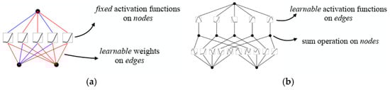
Figure 1.
Shallow model of MLP and KAN. (a) MLP. (b) KAN.
The inspiration behind KANs stems from the Kolmogorov–Arnold representation theorem:
where are binary functions, while n represents the number of neurons, and is a real function.
KANs eliminate the use of linear parameters entirely, substituting each weight parameter with a univariate function defined through a spline. To realize arbitrary depth within KAN, a simple method involves the combination of MLP principles with KAN concepts:
where k represents the number of KAN layers.
To summarize, KANs enhance this theoretical premise by substituting static activation functions with adaptable ones applied to the weights. Every weight is characterized as a spline function that can be adjusted through learning. This design advancement enables KANs to effectively identify intricate nonlinear correlations by directly refining univariate functions. And the adaptive modeling ability of relationships in data enables better prediction and generalization capabilities than MLP. In addition, KAN decomposes complex functions into simpler components, enabling the efficient processing of large datasets and making it an ideal choice for handling large amounts of information tasks.
2.2. Graph Convolutional Networks
Graph-based convolutional models are neural network frameworks designed explicitly for the analysis of data represented as graphs. This type of architecture excels at revealing complex connections between nodes and understanding the inherent properties of the graph via convolutional operations.
For GCN models, the goal is to learn a function of signals/features on a graph G = (V, E), which takes the following as input:
- (a)
- A compact representation of features xi for every node i, compiled within an N × D feature matrix X (N: number of nodes, D: number of input features).
- (b)
- An illustration of the graph’s layout in a matrix representation, commonly expressed as an adjacency matrix A.
This process generates an output at the node level, represented as an N × F feature matrix, with F indicating the number of features attributed to each node. Furthermore, to derive outputs at the graph level, a specific pooling operation must be implemented.
Each layer within a neural network can be expressed as a function that is nonlinear in nature:
with H(0) = X and H(L) = Z (or z for graph-level outputs), L being the number of layers. The specific models then differ only in how f(⋅,⋅) is chosen and parameterized.
Inspired by a first-order analysis of localized spectral filters on graphs, the work of Kipf et al. led to the development of a multi-layer Graph Convolutional Network defined by the following propagation rule for its layers [32]:
with , where I is the identity matrix and is the diagonal node degree matrix of .
2.3. GraphKAN Layer
The architecture of graph neural networks (GNNs) allows for them to accommodate the features of graphs through a process known as message passing. GNNs are adept at managing data structured like graphs, which encompasses features related to nodes, xv, and relationships between edges, evw. Typically, the characteristics of nodes are indicated by node attributes, while edge attributes illustrate the relationships between nodes using an adjacency matrix representation.
The framework for passing messages in relation to node representation can essentially be categorized into two distinct phases [33]:
(a) Aggregates information from the neighbors. The message function is used to aggregate the neighboring features of the target node, including the target node’s own features , the features of its neighboring nodes , and the edge features connecting it to its neighboring nodes . This aggregation forms a message vector that is then passed to the target node. The formula is as follows:
where is the information received by the node in the next layer t + 1, Mt is the message function, represents the node features in the current layer, N(v) represents the set of neighboring nodes for a node v, represents the node features of the neighboring nodes in the current layer, and represents the edge features from node to node.
(b) Extracts the node representation. An update function processes the node features of the subsequent layer by merging the characteristics from the existing layer’s nodes with the information received via the messaging function. The following equation illustrates this process:
where is the node update function which accepts the initial state of the node along with the incoming message and produces the updated state of the node.
Most approaches employ a Multi-layer Perceptron (MLP) for the purpose of feature extraction. To improve the capability for capturing nonlinearity, an activation function is typically integrated into Phase (b), as mentioned above. Functions like ReLU can restrict the ability to represent information, which may hinder the learning of intricate node characteristics. The phase of obtaining node representations is enhanced by substituting the MLP with KAN for Ut. The process of extracting the new representation can be expressed as follows:
This study presents a GraphKAN layer that utilizes a GCN as its foundation. The following illustrates the equation for the GraphKAN layer that utilizes a GCN:
(a) Message function Mt is as follows:
where deg computes the degree of the node.
(b) Node representation extraction function Ut is as follows:
The B-spline function is utilized as the Φt.
3. The Proposed Approach
This section elaborates on the methodology of an innovative approach for diagnosing bearing faults that leverages the proposed GraphKAN framework, along with a detailed description of its specific structure. A diagram illustrating the process of the fault diagnosis method can be found in the accompanying Figure 2. The detailed procedures are outlined as follows:
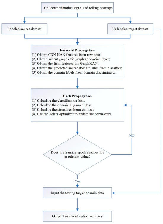
Figure 2.
Flowchart of the proposed approach.
- (a)
- The original signals of rolling bearings are gathered and sampled using an overlapping rectangular sliding window. Each sample must encompass at least a complete cycle of the rolling bearings’ movement signals. These samples consist of one-dimensional time series data representing vibration signals.
- (b)
- These one-dimensional signals are separated into two sections based on a specific ratio: one is the labeled source dataset, while the other is the unlabeled target dataset.
- (c)
- A CNN-KAN architecture is established to derive features from the unprocessed signals, coupled with the introduction of a Graph Generation Layer (GGL) designed to create instance graphs based on the features extracted using the CNN-KAN framework.
- (d)
- The ultimate features are derived through GraphKAN, followed by the computation of losses. The adjustments to the parameters are carried out utilizing the ADAM optimizer. The core idea of the ADAM optimizer is to adaptively adjust the learning rate based on the first-order moment estimate (mean) and second-order moment estimate (variance) of historical gradients.
- (e)
- The data from the target domain, intended for testing, is fed into the pre-trained model to assess the effectiveness of fault diagnosis for rolling bearings.
- (f)
- The results of the diagnostic process are produced.
3.1. The Graph Generation Layer
At its core, a graph consists of two fundamental components: the adjacency matrix A, and the node feature matrix X. To obtain the node feature matrix X, a convolutional neural network is first utilized to extract characteristics from the input data, which can be expressed in the form of the resultant feature maps [28]:
where the matrix represents the input for each mini-batch is located.
An adjacency matrix A has been created using a Generative Graph Generator (GGL), which facilitates the construction of instance graphs based on the mini-batch input data. The initial step involves channeling the feature matrix that results from the extraction phase into a KANLinear layer. Following this, the adjacency matrix is constructed by multiplying the KAN features with their transposed counterparts. Following that, a method rooted in ranking is employed to identify the top K nearest neighbors for each individual node. As a result, the subsequent equation is used to derive the adjacency matrix:
where A represents the constructed adjacency matrix and indicates the results obtained following the KAN process. The function normalize(·) refers to the normalization operation. The matrix in question is a sparse adjacency matrix, and the function Top—k(·) identifies the indices corresponding to the top-k largest entries in each row of A. This approach leads to a sparser form of the adjacency matrix and mitigates computational demands.
3.2. The Loss for the Proposed Approach
The proposed approach is made up of three distinct elements: the feature extraction unit (F), the domain evaluation module (D), and the classification unit (C). In order to support the extraction of adaptable characteristics and effectively capture the essential types of information described earlier, the complete objective function is formed by three key components: the classification loss, the loss related to domain synchronization, and the loss that focuses on structural alignment.
3.2.1. Classification Loss
In order to enhance the accuracy of predictions made by the label classifier, the variation in categorization between the true labels and the predicted ones is assessed utilizing cross-entropy loss, represented mathematically as follows:
where x represents the output of the model, y represents the true label, C represents the number of categories, and n represents the number of samples.
3.2.2. Domain Alignment Loss
When there is a shift in domain covariance, a classifier trained exclusively on data from the source domain often shows inadequate performance on data from the target domain. To tackle this issue, a discriminator (D) is employed to distinguish features originating from the source domain from those sourced from the target domain, while the feature extractor undergoes modifications to effectively counter the discriminator’s assessments. As the competitive dynamics evolve between the two entities, it becomes feasible to pinpoint features that remain constant across different domains. Within this framework, the function utilized for domain alignment is characterized as the binary cross-entropy loss, defined as follows:
3.2.3. Structure Alignment Loss
In order to align the structural characteristics of both the source and target domains, the CORAL loss functions as a loss for aligning the discrepancies in the structure, which can be mathematically expressed in the following manner:
where denotes the squared matrix Frobenius norm. The covariance matrices of the source and target data are given as follows:
where 1 is a column vector with all elements equal to 1.
3.2.4. Overall Loss
By integrating the three established loss functions, one can express the comprehensive objective function required for accomplishing UDA as follows:
where γ and κ are the tradeoff parameters.
Let θF, θC, and θD denote the parameters related to the feature extraction module, the label classification module, and the domain distinction module, respectively. In the model’s training process, the parameters for each part of the approach can be modified through the backpropagation (BP) technique, which is expressed as follows:
where ∂ represents the partial derivative operator and η denotes the learning rate.
3.3. The Architecture of the Proposed Model
As shown in Figure 3, initially, a CNN integrated with a KANLinear layer is utilized to extract relevant features from the input signals. Subsequently, a layer dedicated to graph generation (GGL) is introduced to extract the underlying data architecture from the features obtained via CNN-KAN, facilitating the formation of instance graphs by exploring the interrelations among the structural attributes of the samples. Subsequently, the GraphKAN framework is employed to capture the instance graphs by effectively modeling the structural details that traverse the weighted connections within the graph. In order to assess the differences in structure between the target and source domains, the loss function known as correlation alignment (CORAL) is utilized. Table 1 illustrates the specific parameters associated with the proposed model, and Table 2 shows parts of the hyperparameters.
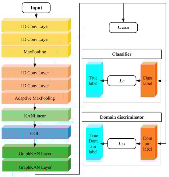
Figure 3.
The architecture of the proposed model.

Table 1.
The proposed model’s detailed parameters.
Table 2.
Hyperparameters of the proposed model.
4. Experimental Verification
In this study, two distinct datasets related to rolling bearings are utilized to demonstrate the effectiveness of the proposed method for fault diagnosis. The experimental arrangement is equipped with a MECHREVO (Beijing, China) laptop with AMD R9-7945HX CPU, a GeForce RTX 4070 GPU, and 32 GB of RAM.
4.1. Experiment Analysis with the HUST Bearing Dataset
4.1.1. Experimental Setup
The HUST dataset pertaining to bearings was developed by Nguyen Duc Thuan et al. at the University of Science and Technology [34]. It encompasses various types of bearing failures occurring under different operational scenarios. As shown in Figure 4, the setup features an induction motor rated at 750 W (1 HP), which powers a multi-step shaft alongside a Leroy Somer powder brake. An inverter regulates the motor, while the powder brake serves as a simulated load. Additionally, the shaft is equipped with a torque sensor and a dynamometer to assess the load and speed of the motor. Various types of housings can accommodate damaged bearings, and these housings are designed to be easily interchangeable on the multi-step shaft. An accelerometer, specifically the PCB 325C33 model, is fitted on the bearing in a vertical orientation to detect vibrations.
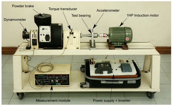
Figure 4.
The test bench of the HUST dataset.
The system for gathering data encompasses a sensor for acceleration, a module for measurement, an enclosure, and software from Labview [34]. The previously mentioned components collectively form a completely automated system for capturing measurement data. The analog signals associated with vibration from the sensor are directed towards the NI-9234 sound and vibration input module, which facilitates the conversion from analog to digital. The signals that have been digitized by the NI-9234 undergo synchronization and conditioning through the NI-CompactDAQ chassis before being transmitted to the software via USB. Vibration data are processed, visualized, and captured within the software environment. The software defines the layout of the measurement unit and the casing.
A collection of 99 unprocessed vibration signals were gathered, capturing six distinct defect types (including inner crack, outer crack, ball crack, and two-combination pairs) across five bearing models (6204, 6205, 6206, 6207, and 6208) under three different operational settings (0 W, 200 W, and 400 W), as illustrated in Table 3. Figure 5 illustrates the various types of defects present. Vibration signals are recorded at a frequency of 51,200 samples per second over a duration of 10 s.
Table 3.
Detailed description of HUST datasets.
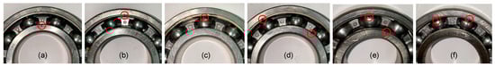
Figure 5.
The defects of bearings. The location of the defects is indicated by red circles. (a) Inner ring. (b) Outer ring. (c) Ball. (d) Inner ring and outer ring. (e) Inner ring and ball. (f) Outer ring and ball.
4.1.2. Experiment Results and Discussion
The collected data were subjected to processing through the application of Z-score normalization methods. Following this, the raw vibration data undergoes segmentation through a sliding window method with a width of 1024, ensuring that the individual samples do not overlap during this step. In total, 500 samples are generated for every health condition, culminating in a comprehensive dataset of 3500 samples encompassing seven distinct health conditions. In addition, to formulate the dataset intended for a particular operational context, a random selection of 80% from each health category is utilized for training, leaving the remaining 20% allocated for testing. As a result, a total of 2800 samples are allocated for training under each distinct operating condition, with 700 samples set aside for testing, as shown in Table 4. The operational modes are identified as A, B, and C, which correspond to the power levels of 0 W, 200 W, and 400 W, respectively. In total, six distinct tasks across various fields are executed to facilitate a thorough assessment.
Table 4.
The number of samples.
In order to showcase the advantages of the suggested CNN-KAN + GraphKAN framework, two contrasting methods are employed, namely, CNN-MLP + GCN and CNN-MLP + GraphKAN. In these comparative models, features are extracted using the CNN-MLP prior to the application of GGL, as illustrated in Table 5. To assess this experiment, various evaluation metrics were applied, focusing on the overall accuracy. The final outcomes are determined by averaging the results from the last ten epochs, which helps minimize variability. The findings from this experiment can be found in the accompanying table. Table 4 displays the outcomes of the experiment, while Figure 6. illustrates the corresponding histogram.
Table 5.
The differences in three models.
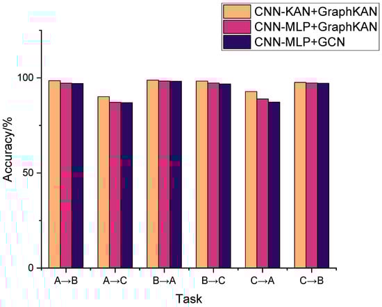
Figure 6.
Comparison of different models.
It can be seen from Table 6 and Figure 6 that the CNN-KAN + GraphKAN approach demonstrates superior performance across all cross-domain tasks. In the most difficult task, Task A→C, the lowest accuracy attained by the least effective model is 86.97%; the proposed method demonstrates a diagnostic accuracy of 90.16%. In the most straightforward task, Task B→A, the least effective model manages to reach a diagnostic accuracy of 98.2%; in contrast, CNN-KAN + GraphKAN attains an accuracy of 98.8%. These findings suggest that the introduced approach is capable of enhancing performance even as domain differences increase and cross-domain tasks become more challenging. Furthermore, CNN-MLP + GraphKAN outperforms CNN-MLP + GCN, demonstrating its superior performance. This suggests that MLP could be substituted with an alternative approach; KAN’s effectiveness has been proven.
Table 6.
Comparison of three models.
Rolling bearings are accompanied by a large amount of environmental noise during operation, varying in degree. The noise has a significant impact on the fault diagnosis results. Therefore, we added varying degrees of noise to the original dataset to evaluate the diagnostic performance and robustness of the proposed model on input signals with different Signal to Noise Ratios (SNRs). The definition of SNR is as follows:
where Psignal and Pnoise are the energy of signal and noise, respectively.
As shown in Table 7, when the SNR is between 10 db and 5 db, the diagnostic accuracy of the model does not decrease significantly. When the SNR reaches 1 db, the diagnostic accuracy of the model shows a significant decrease. The experiments have shown that the proposed model can maintain diagnostic accuracy when the SNR is greater than 5 db.
Table 7.
The accuracy of the proposed model for task A→C under different SNRs.
4.2. Experiment Analysis with the CWRU Dataset
4.2.1. Experimental Setup
The bearing dataset that is accessible to the public from Case Western Reserve University (CWRU) is widely acknowledged as a benchmark dataset for diagnosing bearing failures, which provides an objective assessment of the performance and advantages of various diagnostic techniques [35]. As shown in Figure 7, the equipment incorporates a 2-horsepower electric motor, a power measurement device, and a torque sensor with a decoder, along with the necessary electrical control systems. The focus of this investigation is the SKF rolling bearing model 6205-2 RS JEM located at the drive end. Four distinct bearing conditions were represented, which included a defect in the inner ring, a defect in the outer ring, a defect in the rolling element, and a state with no defects. A relevant illustration can be found in the accompanying Figure 8. Using electrical discharge machining techniques, three distinct categories of single-point faults were established on the inner, outer, and rolling components of the test bearing, each exhibiting different levels of severity. The sizes of the damages were measured at 0.007, 0.014, and 0.021 inches, as shown in Table 8. Vibration acceleration signals are gathered through an acceleration sensor positioned at both the motor fan end and the drive end, operating with a sampling rate of 12 kHz.
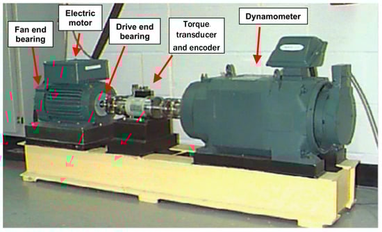
Figure 7.
CWRU bearing test rig.
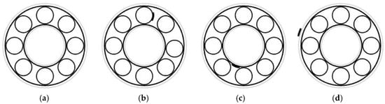
Figure 8.
Rolling bearing fault types. (a) Normal. (b) Ball fault. (c) Inner race fault. (d) Outer race fault.
Table 8.
Details of the CWRU dataset.
Data on vibrations was gathered using accelerometers, which were secured onto the casing with magnetic mounts. The sensors were positioned at the 12 o’clock orientation on both ends of the motor casing, specifically at the drive end and the fan end. In the course of certain trials, an accelerometer was also mounted on the base plate supporting the motor. Vibration data were recorded by utilizing a 16-channel digital audio tape recorder, and digital information was gathered at a rate of 12,000 samples per second, later analyzed using the Matlab platform along with data gathered at a rate of 48,000 samples per second, specifically focusing on the faults of the drive-end bearing. Information regarding speed and horsepower was measured using the torque transducer/encoder and was documented manually.
4.2.2. Experiment Results and Discussion
To further substantiate the results, experiments involving transfer learning with the CWRU dataset have been conducted. The findings, which emphasize the success of transfer learning techniques, are represented in Figure 9 and Table 9, where the indication 0→1 denotes that the data corresponding to the 0hp payload (1797 rpm) functions as the source domain, whereas the data for the 1 hp payload (1772 rpm) is designated as the target domain; meanwhile, the indication 2→3 signifies that the information from the 2 hp load (1750 rpm) is regarded as the source domain, in contrast to the data from the 3 hp load (1730 rpm), which is considered the target domain.
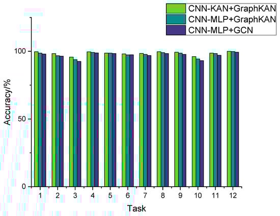
Figure 9.
Comparison of accuracy of different methods.
Table 9.
Comparison of accuracy of different methods.
The findings from this experiment can be found in Table 9. Figure 9 illustrates the histogram. The findings indicate that the suggested approach achieves the highest level of diagnostic precision, aligning with the outcomes observed in earlier experiments. The overall accuracy observed in this experiment surpasses that of the earlier trials, primarily because the CWRU dataset lacks the composite faults present in the HUST dataset. The implementation of the KAN layer, as an alternative to the MLP layer, produced superior outcomes.
As shown in Figure 10a, the classifications within the target domain are effectively separated into ten distinct groups, showcasing notable performance in differentiation. As seen in Figure 10b, it is evident that the features belonging to the same category in both the source and target domains are effectively aligned. The findings indicate that the developed framework effectively captures features that are invariant across domains as well as those that can differentiate them, which are crucial for achieving successful domain adaptation.
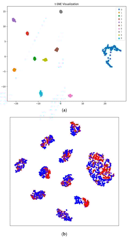
Figure 10.
Feature visualization results by t-SNE of Task 12. (a) The target domain. (b) The source domain and the target domain. Red denotes the source features and blue denotes the target features.
The Friedman test was conducted for statistical significance testing using the results in Table 6 and Table 9. It is a rank-based test that assumes that the mean ranking of all samples is equal. Specifically, different algorithms are first ranked on each dataset, and then the mean ranking of each algorithm on all datasets is calculated. If all algorithms have no performance difference, their average ranking of performance should be equal so that we can choose a specific confidence interval to determine whether the difference is significant. The result of the Friedman test is p = 2.5913565409912746 × 10⁻⁹ < 0.05, which means that there is a significant difference between the three algorithms. The Nemenyi test was then performed for further analysis. As shown in Table 10, the results demonstrate that there are significant differences between the proposed model and every other models.
Table 10.
Results of Nemenyi test.
5. Conclusions
This study introduces an innovative method leveraging GraphKAN for diagnosing faults in rolling bearings amid varying operational scenarios. A framework that integrates CNN and KAN is developed to extract features from the original signals, accompanied by the introduction of a Graph Generation Layer (GGL) that formulates instance graphs using the CNN-KAN features. This design effectively merges the robust feature extraction efficiency of a CNN with the comprehensive generalization abilities of a GCN, addressing the challenges posed by domain shifts in varying operational scenarios. In the proposed framework, KAN layers substitute the conventional MLP layers within the GCN architecture, facilitating a more effective synthesis of both local and global information found in the graphs, which enhances the overall functionality of the approach. Results from experiments conducted on two bearing datasets indicate that the methodology proposed has achieved superior accuracy in fault diagnosis and enhanced stability in varying operational conditions when compared to alternative techniques.
Nonetheless, enhancements to the efficacy of the suggested method could be achieved through the following considerations: (a) the existing classifier and discriminator utilize MLP, which could be substituted with KAN; (b) a comparison of domain adaptation techniques may be conducted.
Author Contributions
Conceptualization, Y.L. and X.N.; methodology, Y.X. and H.Q.; software, Y.L.; validation, Y.X. and J.L.; formal analysis, J.L.; investigation, Y.X. and H.Q.; resources, X.N.; data curation, J.L.; writing—original draft preparation, Y.L.; writing—review and editing, Y.X.; visualization, X.N.; supervision, J.L.; project administration, X.N. and H.Q.; funding acquisition, Y.X. All authors have read and agreed to the published version of the manuscript.
Funding
This research was funded by National Natural Science Foundation of China (NSFC) (No. 52479082) and Theories and methods for wide area forecast and panoramic operation in the mesoscale flood control system of the Upper Yangtze River (No. 52039004).
Institutional Review Board Statement
Not applicable.
Informed Consent Statement
Not applicable.
Data Availability Statement
The data are publicly available. The HUST dataset is available at https://doi.org/10.17632/cbv7jyx4p9 (accessed on 10 October 2024), and the CWRU dataset is available at https://engineering.case.edu/bearingdatacenter/download-data-file (accessed on 20 October 2024).
Acknowledgments
We would like to thank all the workmates who participated in the work in the School of Civil and Hydraulic Engineering, Huazhong University of Science and Technology.
Conflicts of Interest
The authors declare no conflicts of interest.
References
- Zhang, Z.; Huang, W.; Liao, Y.; Song, Z.; Shi, J.; Jiang, X.; Shen, C.; Zhu, Z. Bearing Fault Diagnosis via Generalized Logarithm Sparse Regularization. Mech. Syst. Signal Process. 2022, 167, 108576. [Google Scholar] [CrossRef]
- Li, H.; Lv, Y.; Yuan, R.; Dang, Z.; Cai, Z.; An, B. Fault Diagnosis of Planetary Gears Based on Intrinsic Feature Extraction and Deep Transfer Learning. Meas. Sci. Technol. 2023, 34, 014009. [Google Scholar] [CrossRef]
- Liu, R.; Yang, B.; Zio, E.; Chen, X. Artificial Intelligence for Fault Diagnosis of Rotating Machinery: A Review. Mech. Syst. Signal Process. 2018, 108, 33–47. [Google Scholar] [CrossRef]
- Yang, C.; Zhou, K.; Liu, J. SuperGraph: Spatial-Temporal Graph-Based Feature Extraction for Rotating Machinery Diagnosis. IEEE Trans. Ind. Electron. 2022, 69, 4167–4176. [Google Scholar] [CrossRef]
- Lei, Y.; Jia, F.; Lin, J.; Xing, S.; Ding, S.X. An Intelligent Fault Diagnosis Method Using Unsupervised Feature Learning Towards Mechanical Big Data. IEEE Trans. Ind. Electron. 2016, 63, 3137–3147. [Google Scholar] [CrossRef]
- Chen, Z.; Mauricio, A.; Li, W.; Gryllias, K. A Deep Learning Method for Bearing Fault Diagnosis Based on Cyclic Spectral Coherence and Convolutional Neural Networks. Mech. Syst. Signal Process. 2020, 140, 106683. [Google Scholar] [CrossRef]
- Chen, Y.; Zhang, T.; Luo, Z.; Sun, K. A Novel Rolling Bearing Fault Diagnosis and Severity Analysis Method. Appl. Sci. 2019, 9, 2356. [Google Scholar] [CrossRef]
- Fu, W.; Jiang, X.; Li, B.; Tan, C.; Chen, B.; Chen, X. Rolling Bearing Fault Diagnosis Based on 2D Time-Frequency Images and Data Augmentation Technique. Meas. Sci. Technol. 2023, 34, 045005. [Google Scholar] [CrossRef]
- He, X.; Wang, D.; Li, Y.; Zhou, C. A Novel Bearing Fault Diagnosis Method Based on Gaussian Restricted Boltzmann Machine. Math. Probl. Eng. 2016, 2016, 2957083. [Google Scholar] [CrossRef]
- Pan, T.; Chen, J.; Pan, J.; Zhou, Z. A Deep Learning Network via Shunt-Wound Restricted Boltzmann Machines Using Raw Data for Fault Detection. IEEE Trans. Instrum. Meas. 2020, 69, 4852–4862. [Google Scholar] [CrossRef]
- Dao, F.; Zeng, Y.; Qian, J. Fault Diagnosis of Hydro-Turbine via the Incorporation of Bayesian Algorithm Optimized CNN-LSTM Neural Network. Energy 2024, 290, 130326. [Google Scholar] [CrossRef]
- Hsueh, Y.-M.; Ittangihal, V.R.; Wu, W.-B.; Chang, H.-C.; Kuo, C.-C. Fault Diagnosis System for Induction Motors by CNN Using Empirical Wavelet Transform. Symmetry 2019, 11, 1212. [Google Scholar] [CrossRef]
- Zhao, Z. A Semi-Supervised Gaussian Mixture Variational Autoencoder Method for Few-Shot Fine-Grained Fault Diagnosis. Neural Netw. 2024, 178, 106482. [Google Scholar] [CrossRef]
- Yu, F.; Liu, J.; Liu, D.; Wang, H. Supervised Convolutional Autoencoder-Based Fault-Relevant Feature Learning for Fault Diagnosis in Industrial Processes. J. Taiwan Inst. Chem. Eng. 2022, 132, 104200. [Google Scholar] [CrossRef]
- Jia, G.; Meng, Y.; Qin, Z. Bearing Fault Diagnosis Based on Optimized Feature Mode Decomposition and Improved Deep Belief Network. SDHM 2024, 18, 445–463. [Google Scholar] [CrossRef]
- Tang, J.; Wu, J.; Qing, J. A Feature Learning Method for Rotating Machinery Fault Diagnosis via Mixed Pooling Deep Belief Network and Wavelet Transform. Results Phys. 2022, 39, 105781. [Google Scholar] [CrossRef]
- Ma, J.; Wang, X. Compound Fault Diagnosis of Rolling Bearing Based on ACMD, Gini Index Fusion and AO-LSTM. Symmetry 2021, 13, 2386. [Google Scholar] [CrossRef]
- Ahsan, M.; Salah, M.M. Efficient DCNN-LSTM Model for Fault Diagnosis of Raw Vibration Signals: Applications to Variable Speed Rotating Machines and Diverse Fault Depths Datasets. Symmetry 2023, 15, 1413. [Google Scholar] [CrossRef]
- Zhang, K.; Tang, B.; Deng, L.; Liu, X. A Hybrid Attention Improved ResNet Based Fault Diagnosis Method of Wind Turbines Gearbox. Measurement 2021, 179, 109491. [Google Scholar] [CrossRef]
- Liu, Y.; Gao, T.; Wu, W.; Sun, Y. Planetary Gearboxes Fault Diagnosis Based on Markov Transition Fields and SE-ResNet. Sensors 2024, 24, 7540. [Google Scholar] [CrossRef]
- Yu, Z.; Zhang, C.; Deng, C. An Improved GNN Using Dynamic Graph Embedding Mechanism: A Novel End-to-End Framework for Rolling Bearing Fault Diagnosis under Variable Working Conditions. Mech. Syst. Signal Process. 2023, 200, 110534. [Google Scholar] [CrossRef]
- Zhang, J.; Sun, Y.; Guo, L.; Gao, H.; Hong, X.; Song, H. A New Bearing Fault Diagnosis Method Based on Modified Convolutional Neural Networks. Chin. J. Aeronaut. 2020, 33, 439–447. [Google Scholar] [CrossRef]
- Fang, H.; Deng, J.; Zhao, B.; Shi, Y.; Zhou, J.; Shao, S. LEFE-Net: A Lightweight Efficient Feature Extraction Network With Strong Robustness for Bearing Fault Diagnosis. IEEE Trans. Instrum. Meas. 2021, 70, 1–11. [Google Scholar] [CrossRef]
- Zou, Y.; Liu, Y.; Deng, J.; Jiang, Y.; Zhang, W. A Novel Transfer Learning Method for Bearing Fault Diagnosis under Different Working Conditions. Measurement 2021, 171, 108767. [Google Scholar] [CrossRef]
- Wu, H.; Li, J.; Zhang, Q.; Tao, J.; Meng, Z. Intelligent Fault Diagnosis of Rolling Bearings under Varying Operating Conditions Based on Domain-Adversarial Neural Network and Attention Mechanism. ISA Trans. 2022, 130, 477–489. [Google Scholar] [CrossRef]
- Ding, X.; Lin, L.; He, D.; Wang, L.; Huang, W.; Shao, Y. A Weight Multinet Architecture for Bearing Fault Classification Under Complex Speed Conditions. IEEE Trans. Instrum. Meas. 2021, 70, 1–11. [Google Scholar] [CrossRef]
- Guo, S.; Zhang, B.; Yang, T.; Lyu, D.; Gao, W. Multitask Convolutional Neural Network With Information Fusion for Bearing Fault Diagnosis and Localization. IEEE Trans. Ind. Electron. 2020, 67, 8005–8015. [Google Scholar] [CrossRef]
- Li, T.; Zhao, Z.; Sun, C.; Yan, R.; Chen, X. Domain Adversarial Graph Convolutional Network for Fault Diagnosis Under Variable Working Conditions. IEEE Trans. Instrum. Meas. 2021, 70, 1–10. [Google Scholar] [CrossRef]
- Zhu, J.; Chen, N.; Shen, C. A New Multiple Source Domain Adaptation Fault Diagnosis Method Between Different Rotating Machines. IEEE Trans. Ind. Inf. 2021, 17, 4788–4797. [Google Scholar] [CrossRef]
- Feng, K.; Wang, D.; Dong, M.; Lou, X.; Zhang, Y.; Deng, C.; Zhu, L. Aircraft Landing Gear Load Prediction Based on LSTM-KAN Network. Opt. Fiber Technol. 2025, 90, 104112. [Google Scholar] [CrossRef]
- Liu, Z.; Wang, Y.; Vaidya, S.; Ruehle, F.; Halverson, J.; Soljačić, M.; Hou, T.Y.; Tegmark, M. KAN: Kolmogorov-Arnold Networks. arXiv 2024, arXiv:2404.19756. [Google Scholar]
- Kipf, T.N.; Welling, M. Semi-Supervised Classification with Graph Convolutional Networks. arXiv 2016, arXiv:1609.02907. [Google Scholar]
- Zhang, F.; Zhang, X. GraphKAN: Enhancing Feature Extraction with Graph Kolmogorov Arnold Networks. arXiv 2024, arXiv:2406.13597. [Google Scholar]
- Thuan, N.D.; Hong, H.S. HUST Bearing: A Practical Dataset for Ball Bearing Fault Diagnosis. BMC Res. Notes 2023, 16, 138. [Google Scholar] [CrossRef] [PubMed]
- Center B D 2013 Case Western Reserve University Bearing Data. Available online: https://Engineering.Case.Edu/Bearingdatacenter/Download-Data-File (accessed on 20 October 2024).
Disclaimer/Publisher’s Note: The statements, opinions and data contained in all publications are solely those of the individual author(s) and contributor(s) and not of MDPI and/or the editor(s). MDPI and/or the editor(s) disclaim responsibility for any injury to people or property resulting from any ideas, methods, instructions or products referred to in the content. |
© 2025 by the authors. Licensee MDPI, Basel, Switzerland. This article is an open access article distributed under the terms and conditions of the Creative Commons Attribution (CC BY) license (https://creativecommons.org/licenses/by/4.0/).