

Angle-Resolved Lattice Population Density Plots: A Novel Approach for Fast 2D Unit Cell Determination from HAADF STEM Images

Abstract
1. Introduction
2. Materials and Methods
2.1. Calculation of Angle-Resolved Lattice Population Density (ALPD) Plots

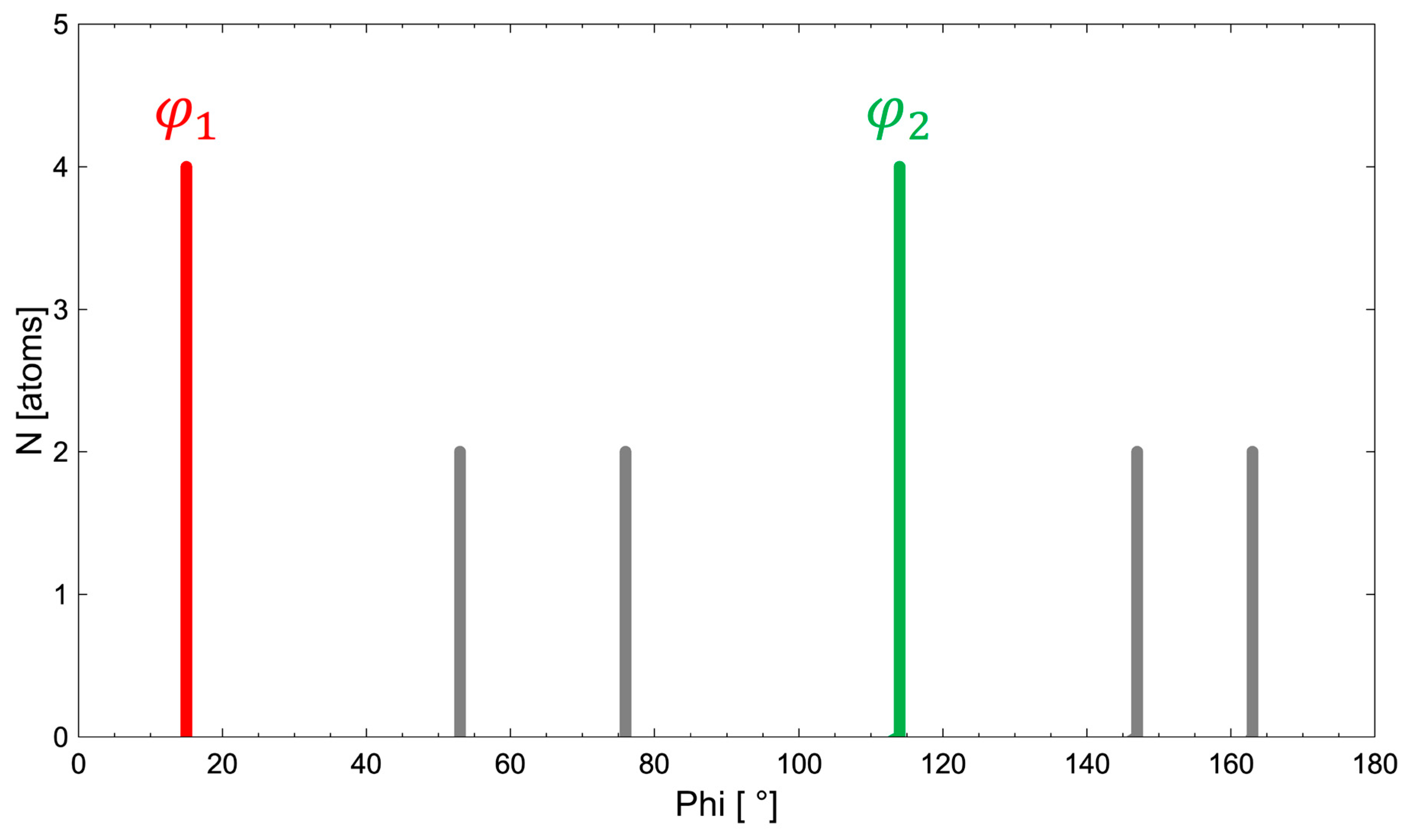
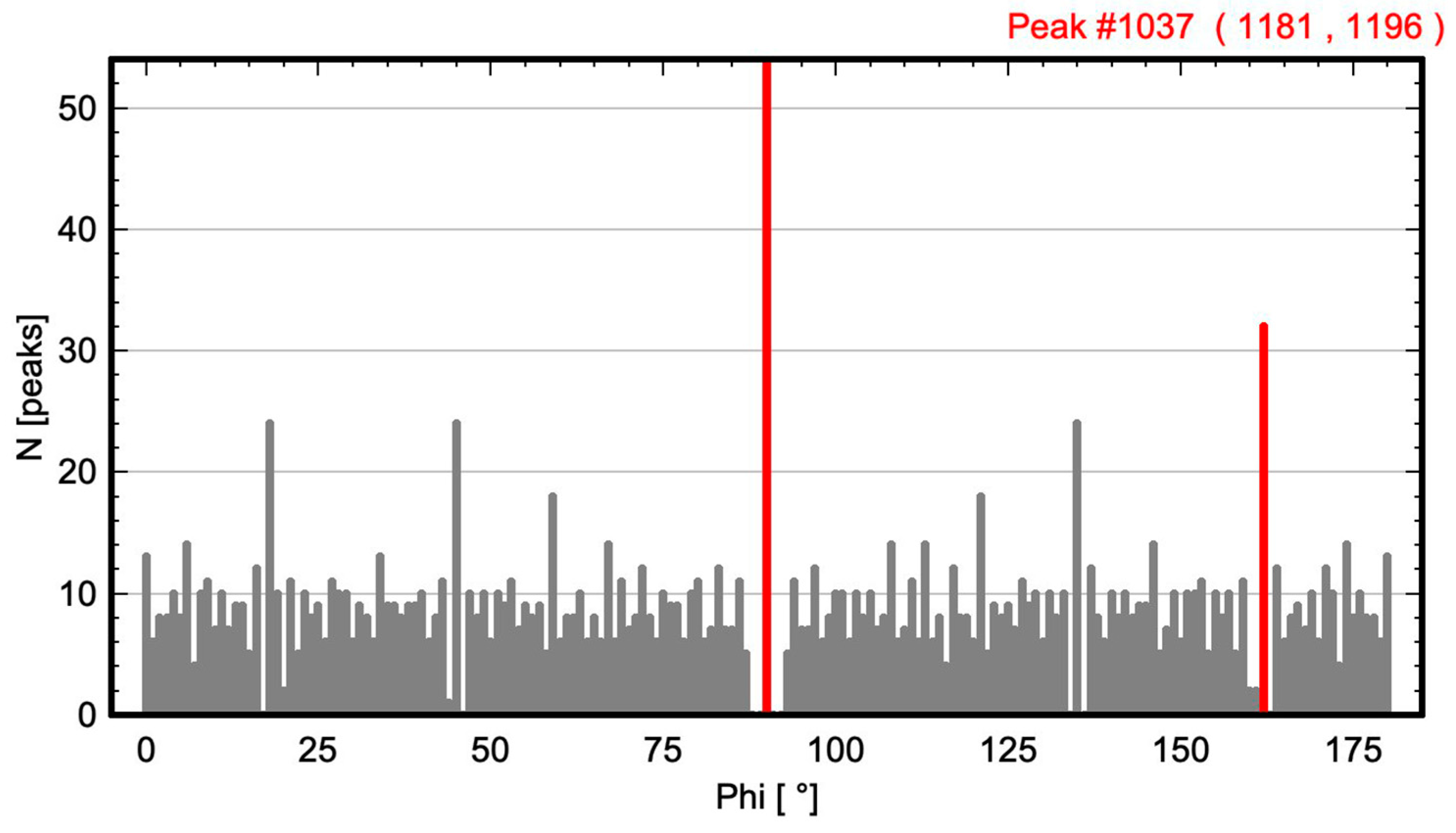
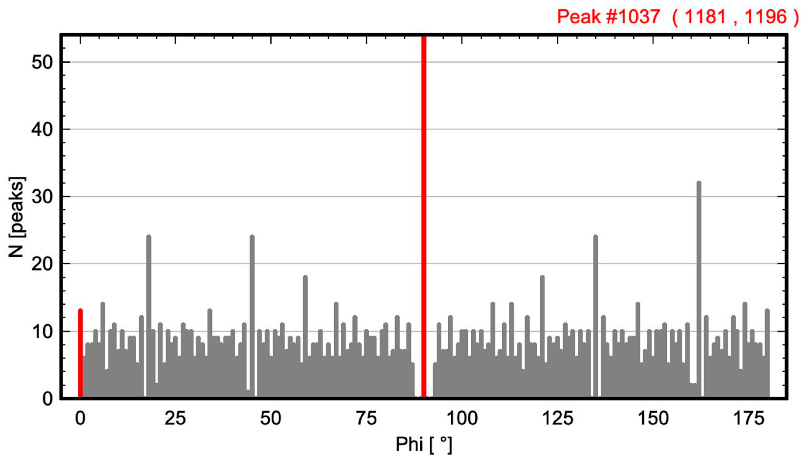
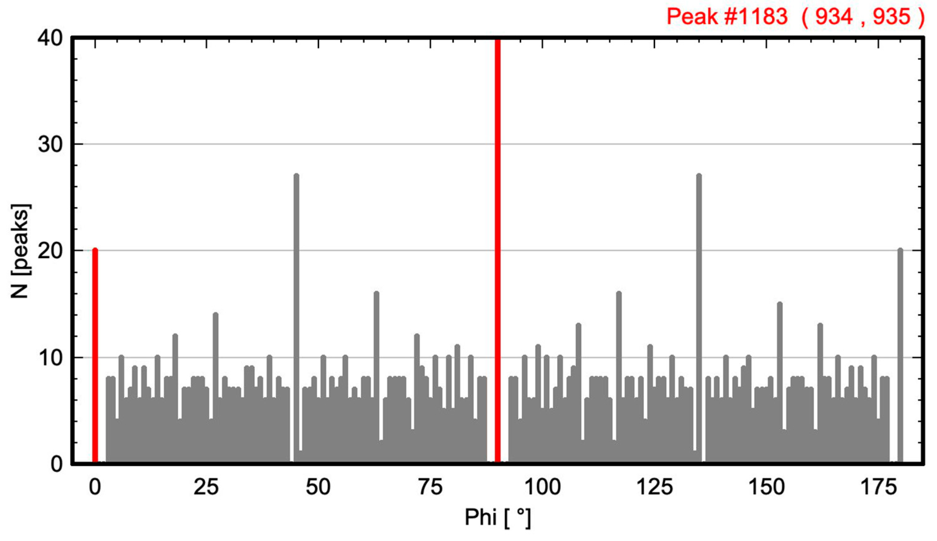
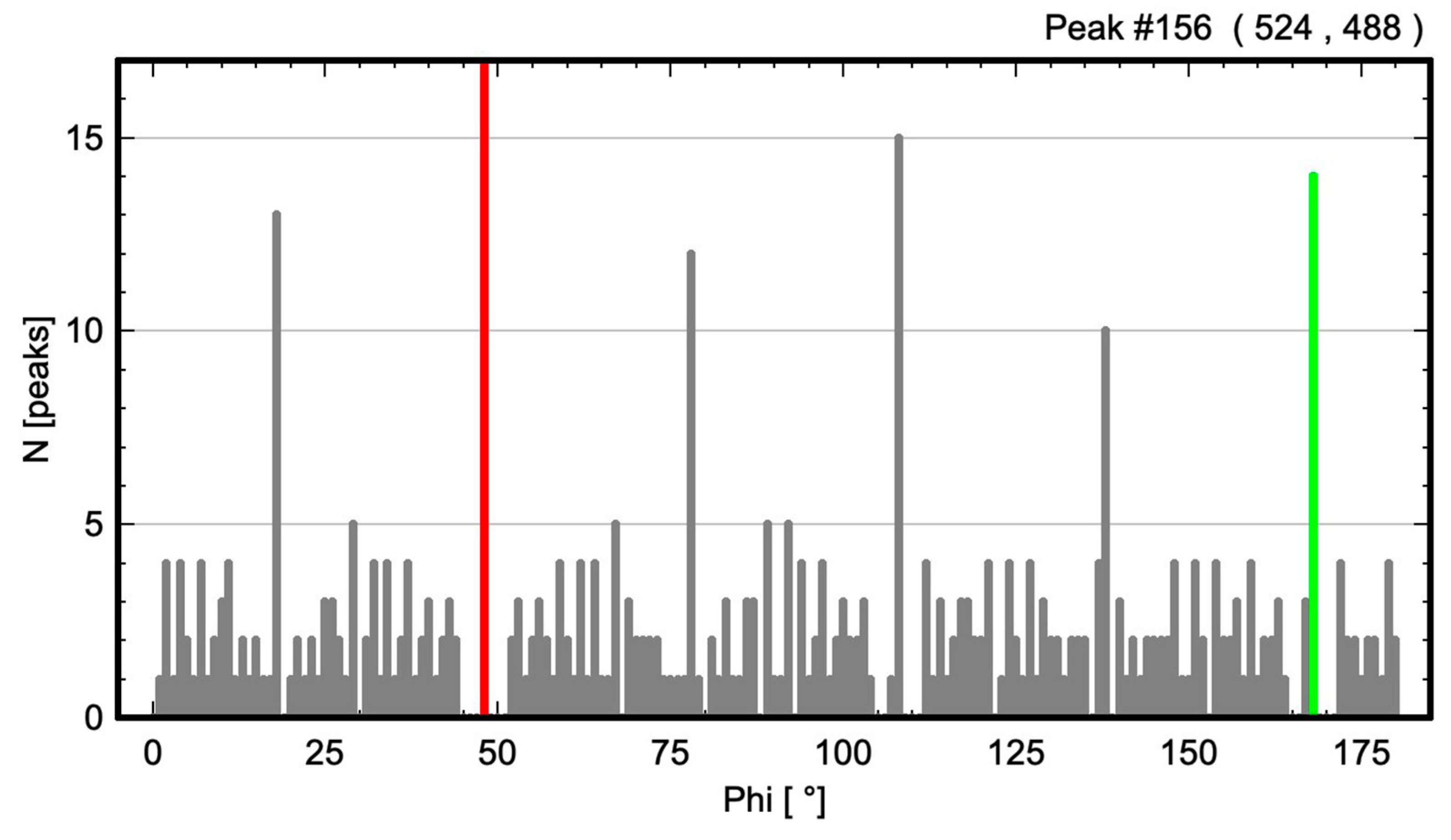
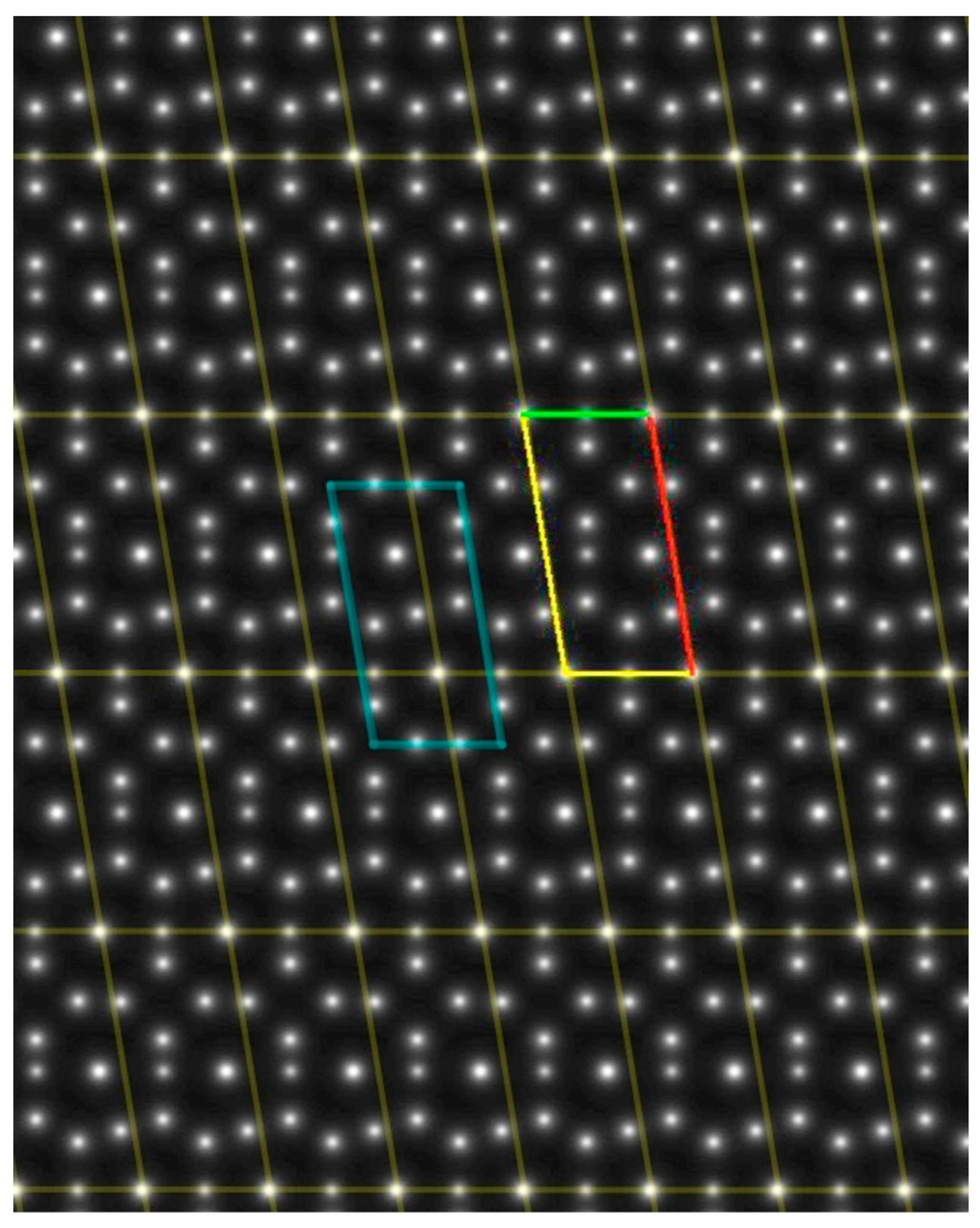
- The angle difference between the two largest maxima in the ALPD plot (lines with the highest atom density) of a monoatomic structure defines the cell angle of the primitive 2D unit cell.
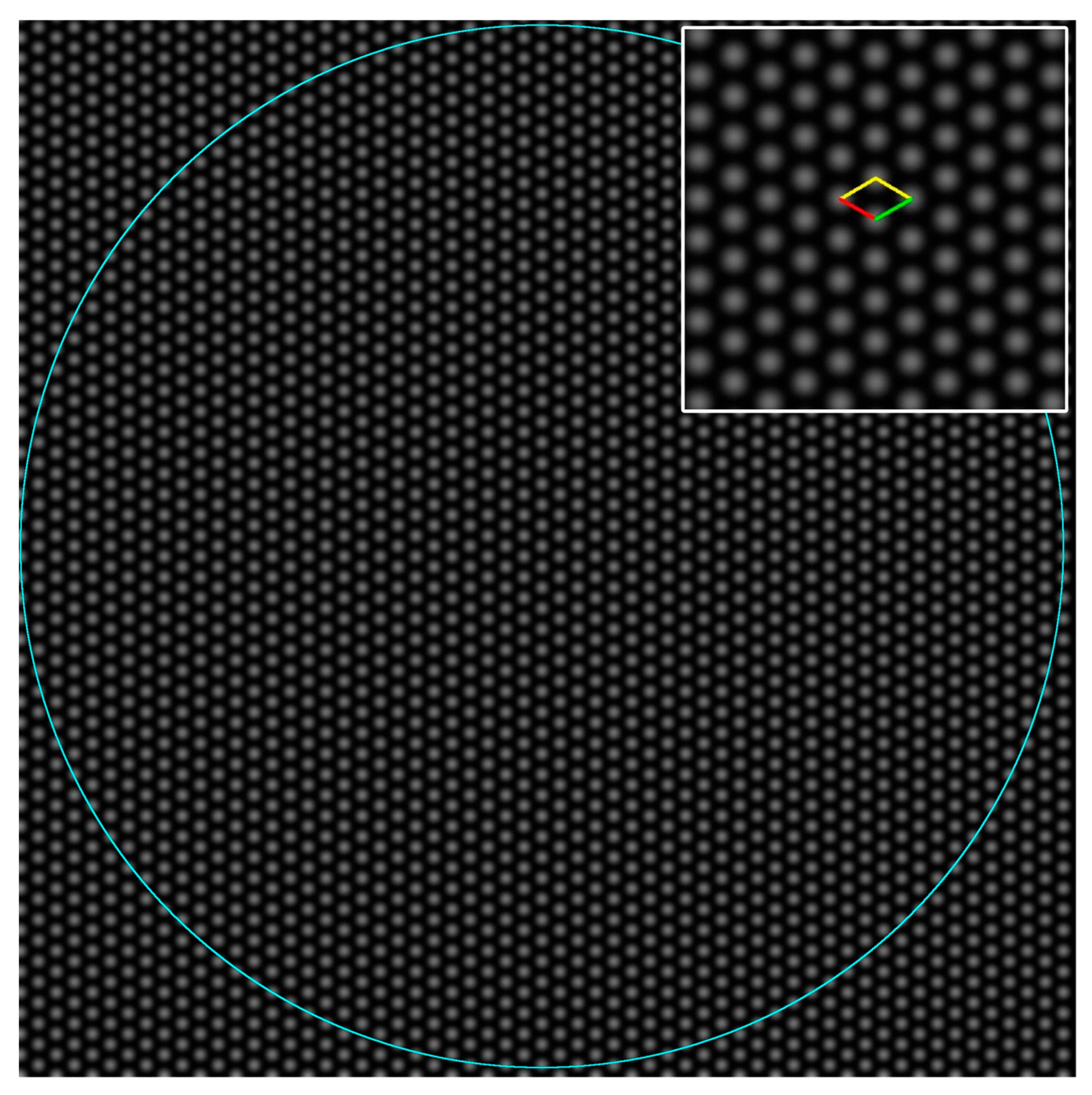
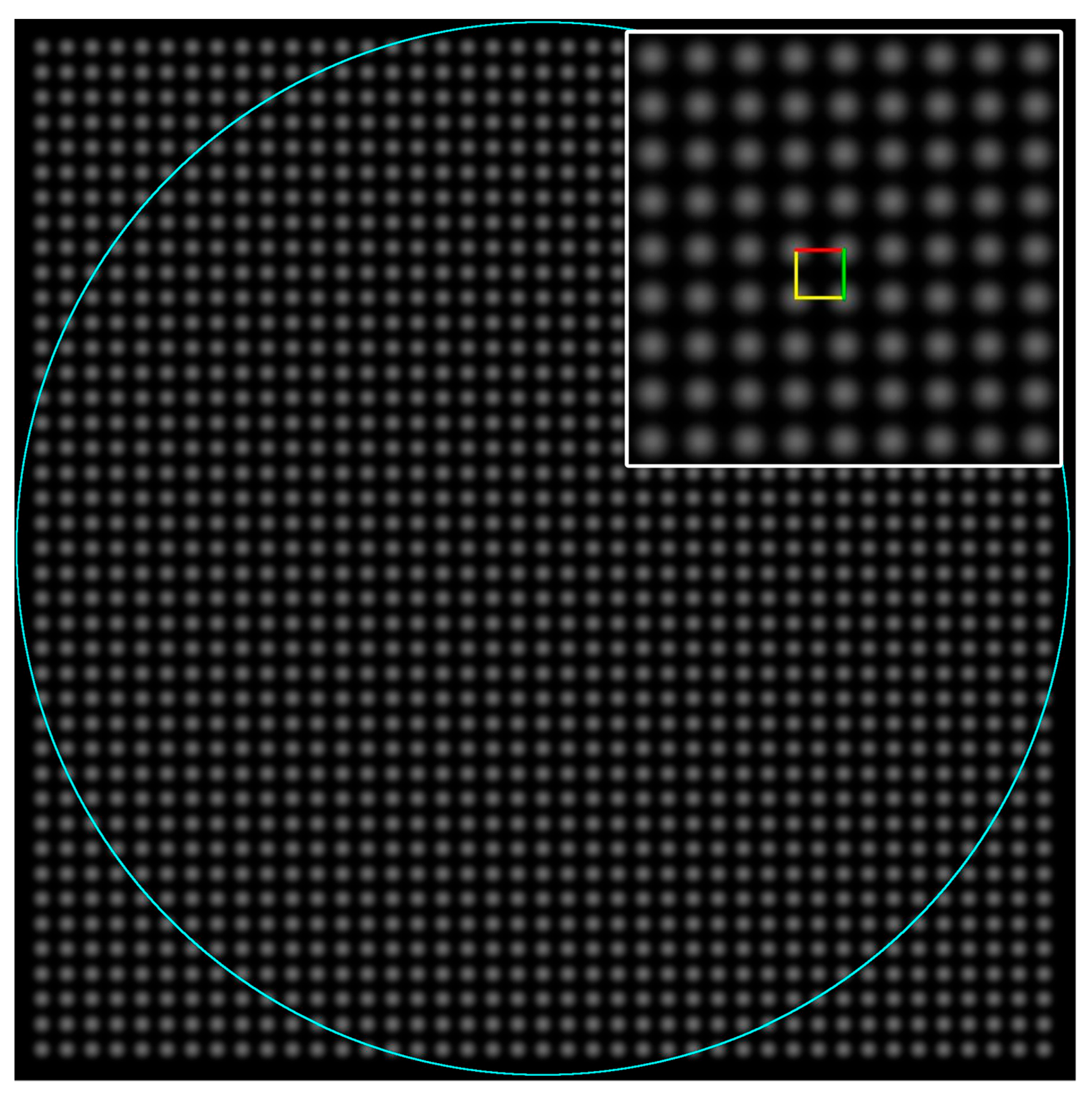
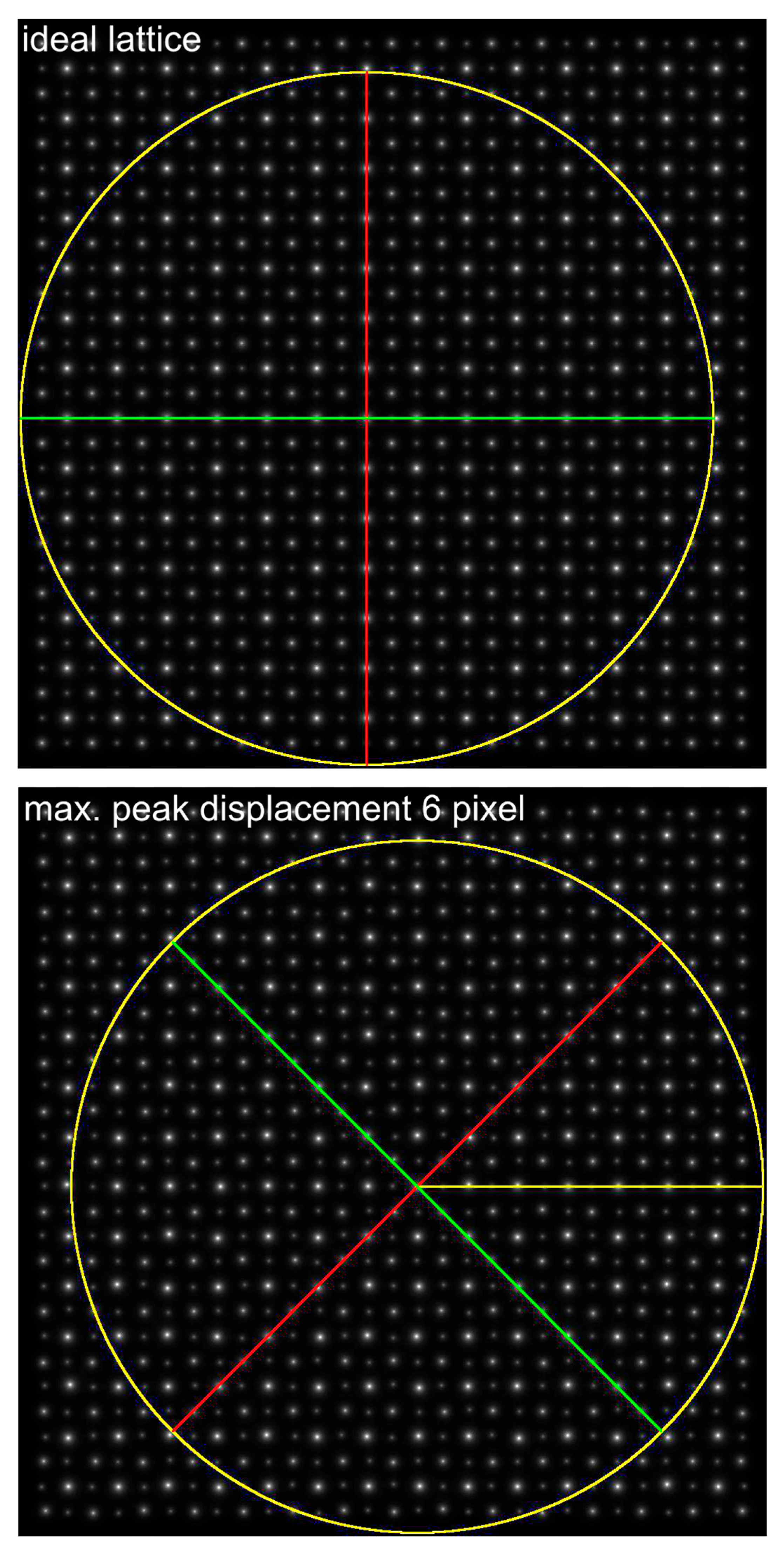
- For a perfect regular primitive lattice, with atoms at all lattice nodes, the lengths of the two axes of the primitive unit cell are given by the distances of the two closest atom peaks along each line to the atom at the origin.
2.2. Test Images and Software

| 2D Lattice Type | Plane Group Symmetry | Number of Peaks Within Maximum Circle | Figure # |
|---|---|---|---|
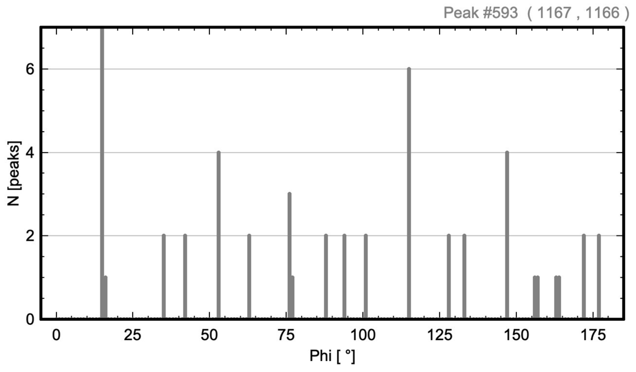
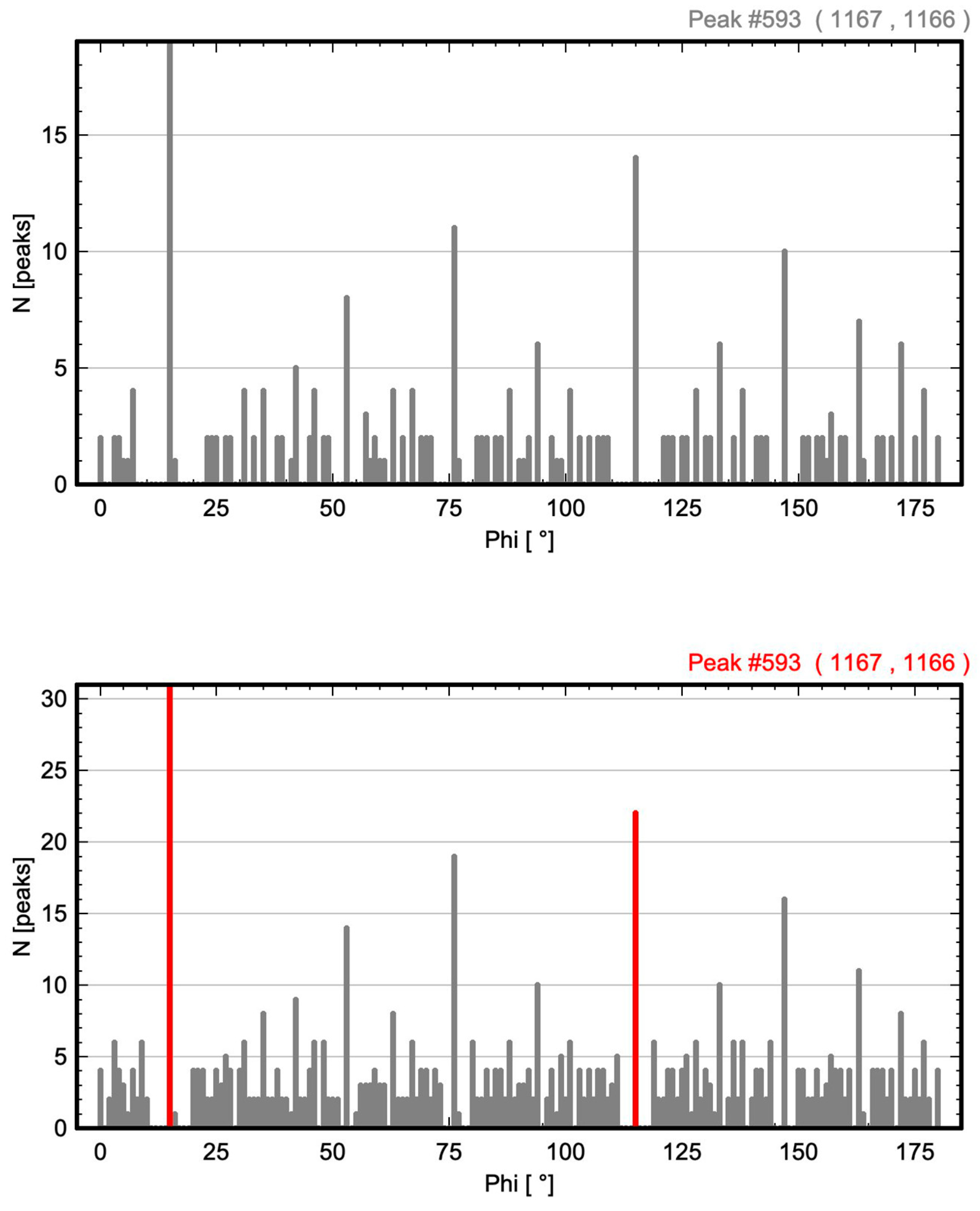
| Oblique P | p2 (no. 2) | 593 | Figure 3 and Figure 4 |
| Rectangular P | p2mm (no. 6) | 672 | Figure 5 and Figure 6 |
| Rectangular C | c2mm (no. 9) | 1576 | Figure 7 and Figure 8 |
| Hexagonal P | p6mm (no. 17) | 2267 | Figure 9 and Figure 10 |
| Square P | p4mm (no. 11) | 929 | Figure 11 and Figure 12 |


2.3. Lattices of Real Crystal Structures
2.3.1. Magnesium
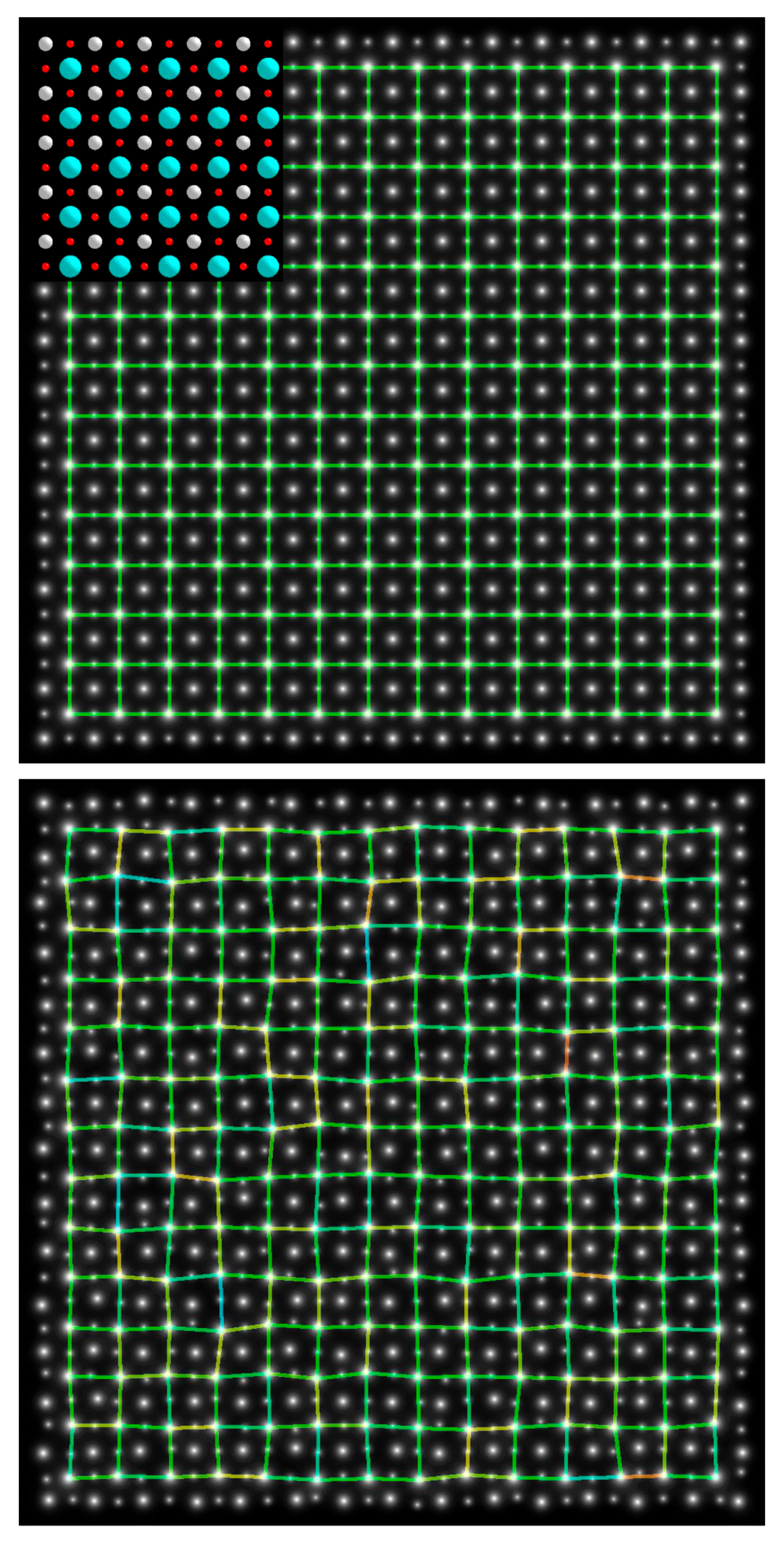
2.3.2. Barium Titanium Oxide, BaTiO3
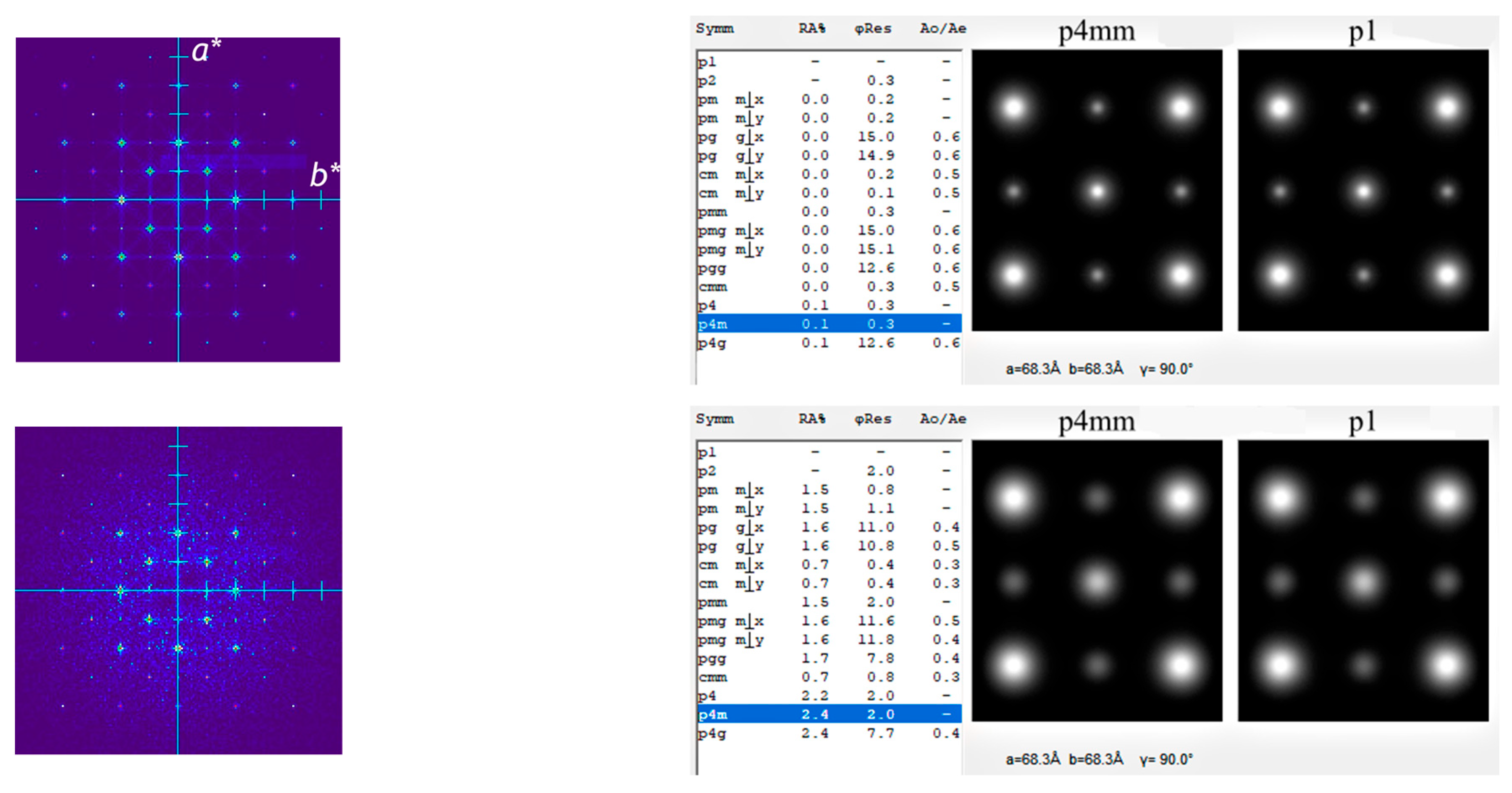
2.4. Comparison with Fourier-Based Crystallographic Image Processing (CIP)
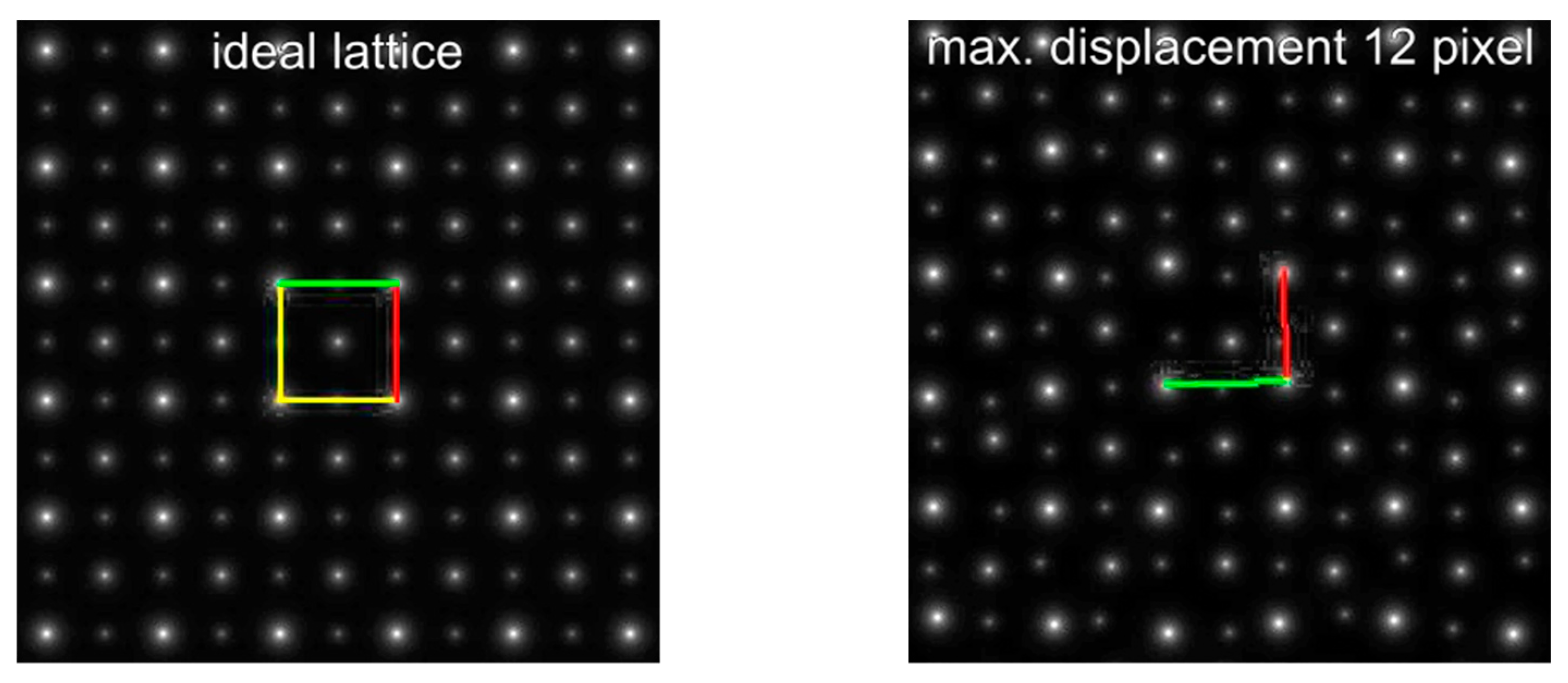
2.5. Comparison with the Real-Space Approach Using Lattice Projections
3. Results
3.1. Oblique P Lattice
3.2. Results from Testing the Higher Symmetry Lattices
3.3. Results from Testing Lattices of Real Crystal Structures
4. Discussion
5. Conclusions
Funding
Data Availability Statement
Conflicts of Interest
References
- Kirkland, E.J. (Ed.) Calculation of Images of Thin Specimens. In Advanced Computing in Electron Microscopy; Springer International Publishing: Berlin/Heidelberg, Germany, 2020; pp. 99–141. [Google Scholar] [CrossRef]
- Heidelmann, M.; Barthel, J.; Cox, G.; Weirich, T.E. Periodic Cation Segregation in Cs0.44[Nb2.54W2.46O14] Quantified by High-Resolution Scanning Transmission Electron Microscopy. Microsc. Microanal. 2014, 20, 1453–1462. [Google Scholar] [CrossRef] [PubMed]
- Ophus, C. Four-Dimensional Scanning Transmission Electron Microscopy (4D-STEM): From Scanning Nanodiffraction to Ptychography and Beyond. Microsc. Microanal. 2019, 25, 563–582. [Google Scholar] [CrossRef] [PubMed]
- Aroyo, M.I. (Ed.) International Tables for Crystallography: Space-Group Symmetry: Vol. A, 2nd ed.; International Union of Crystallography: Chester, UK, 2016; Section 2.1.3.4. [Google Scholar] [CrossRef]
- Hammond, C. The Basics of Crystallography and Diffraction, 2nd ed.; Oxford University Press: Oxford, UK, 2001. [Google Scholar]
- Hovmöller, S. Crystallographic image processing. Micron Microsc. Acta 1992, 23, 181–182. [Google Scholar] [CrossRef]
- Zou, X.; Hovmöller, S. Structure Determination from HREM by Crystallographic Image Processing. In Electron Crystallography; Weirich, T.E., Lábár, J.L., Zou, X., Eds.; Springer: Dordrecht, The Netherlands, 2006; Volume 211, pp. 275–300. [Google Scholar] [CrossRef]
- Gipson, B.; Zeng, X.; Zhang, Z.Y.; Stahlberg, H. 2dx—User-friendly image processing for 2D crystals. J. Struct. Biol. 2007, 157, 64–72. [Google Scholar] [CrossRef]
- Hovmöller, S. CRISP: Crystallographic image processing on a personal computer. Ultramicroscopy 1992, 41, 121–135. [Google Scholar] [CrossRef]
- Alhassan, A.S.A.; Zhang, S.; Berkels, B. Direct motif extraction from high resolution crystalline STEM images. Ultramicroscopy 2023, 254, 113827. [Google Scholar] [CrossRef] [PubMed]
- Momma, K.; Izumi, F. VESTA 3 for three-dimensional visualization of crystal, volumetric and morphology data. J. Appl. Crystallogr. 2011, 44, 1272–1276. [Google Scholar] [CrossRef]
- Schindelin, J.; Arganda-Carreras, I.; Frise, E.; Kaynig, V.; Longair, M.; Pietzsch, T.; Preibisch, S.; Rueden, C.; Saalfeld, S.; Schmid, B.; et al. Fiji: An open-source platform for biological-image analysis. Nat. Methods 2012, 9, 676–682. [Google Scholar] [CrossRef] [PubMed]
- Swanson, H. Circular of the Bureau of Standards No. 539 Volume 1: Standard X-Ray Diffraction Powder Patterns; National Institute of Standards and Technology: Gaithersburg, MD, USA, 1953; pp. 10–11. [Google Scholar] [CrossRef]
- Swanson, H.; Ugrinic, G. Circular of the Bureau of Standards No. 539 Volume 1: Standard X-Ray Diffraction Powder Patterns; National Institute of Standards and Technology: Gaithersburg, MD, USA, 1954; p. 45. [Google Scholar] [CrossRef]
- Galasso, F.S. Structure and Properties of Inorganic Solids, 1st ed.; Pergamon Press: Oxford, UK, 1970; Chapter 7.4; p. 170. [Google Scholar]
- Barthel, J.; Weirich, T.E.; Cox, G.; Hibst, H.; Thust, A. Structure of Cs0.5[Nb2.5W2.5O14] analysed by focal-series reconstruction and crystallographic image processing. Acta Mater. 2010, 58, 3764–3772. [Google Scholar] [CrossRef]
- Hovmöller, S.; Sjögren, A.; Farrants, G.; Sundberg, M. Accurate atom positions from electron microscopy. Nature 1984, 311, 238–241. [Google Scholar] [CrossRef]
- Weirich, T.E.; Ramlau, R.; Simon, A.; Hovmöller, S.; Zou, X. A crystal structure determined with 0.02 Å accuracy by electron microscopy. Nature 1996, 382, 144–146. [Google Scholar] [CrossRef]
- Hunt, C.R.; Raman, A. Alloy chemistry of σ (β-U)-related phases—I. Extension of μ-and occurance of μ’-phases in the ternary systems Nb (Ta)-X-Al (X = Fe, Co, Ni, Cu, Cr, Mo). Z. Für Met. 1968, 59, 701–707. [Google Scholar]
- Nakatani, T.; Yoshiasa, A.; Nakatsuka, A.; Hiratoko, T.; Mashimo, T.; Okube, M.; Sasaki, S. Variable-temperature single-crystal X-ray diffraction study of tetragonal and cubic perovskite-type barium titanate phases. Acta Cryst. 2016, B72, 151–159. [Google Scholar] [CrossRef] [PubMed]
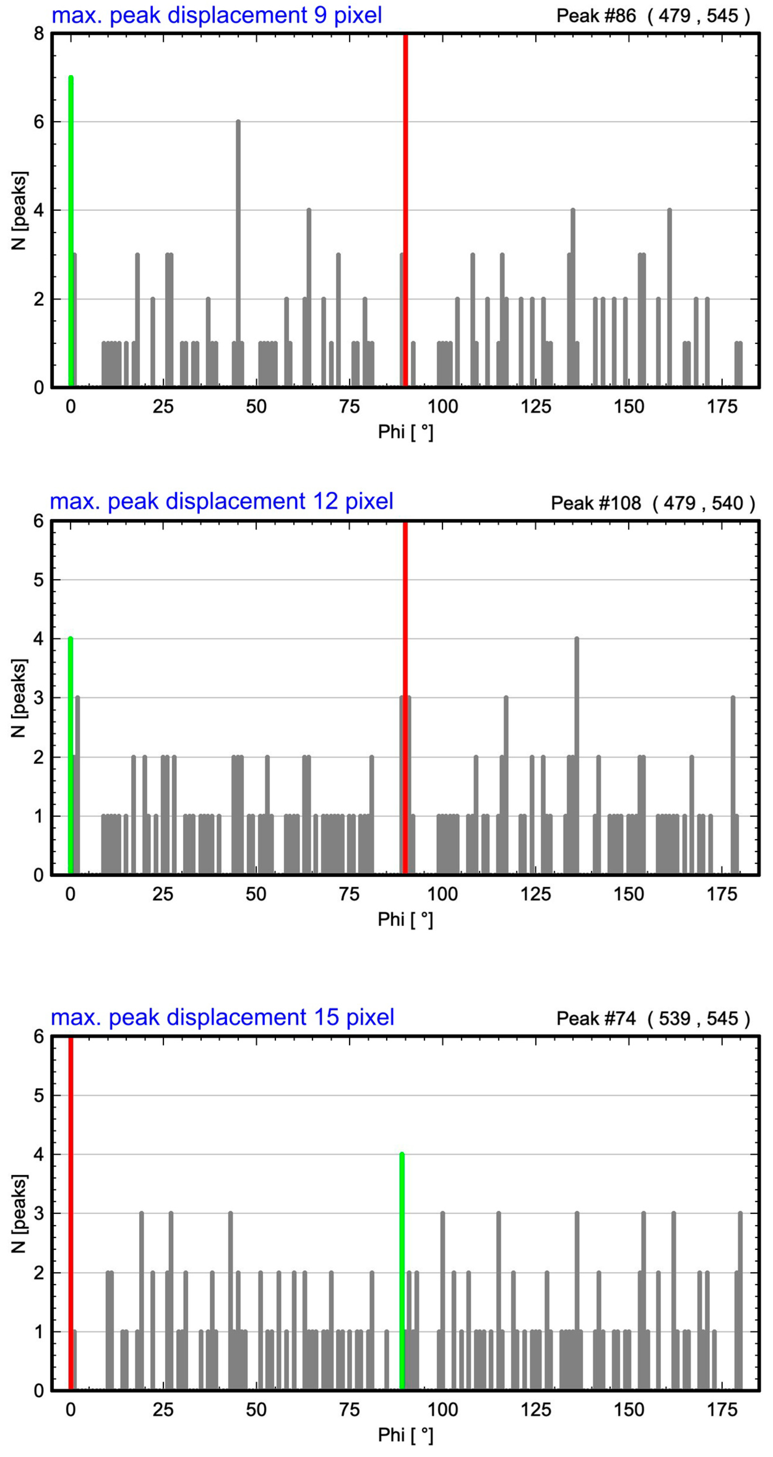
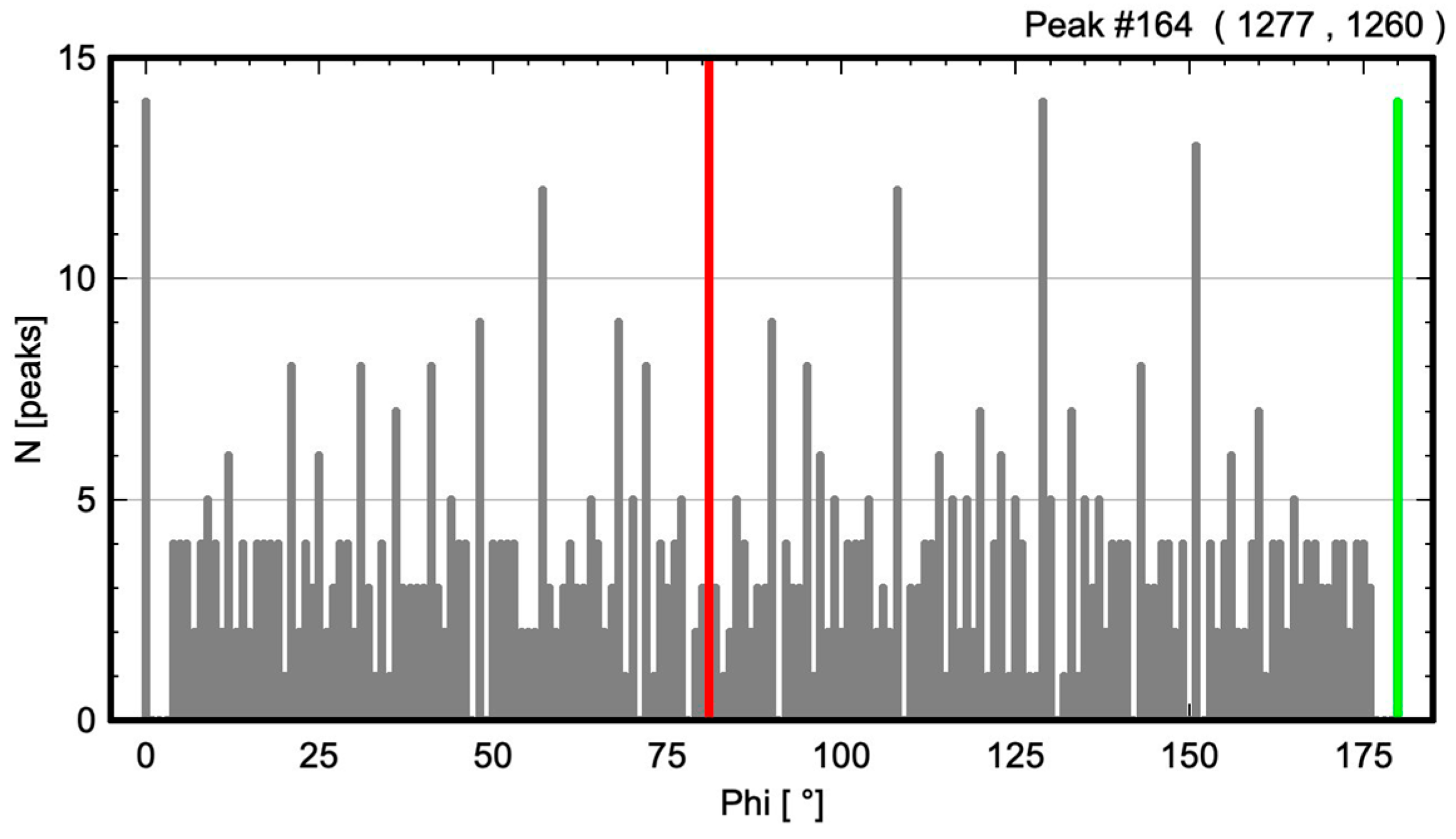
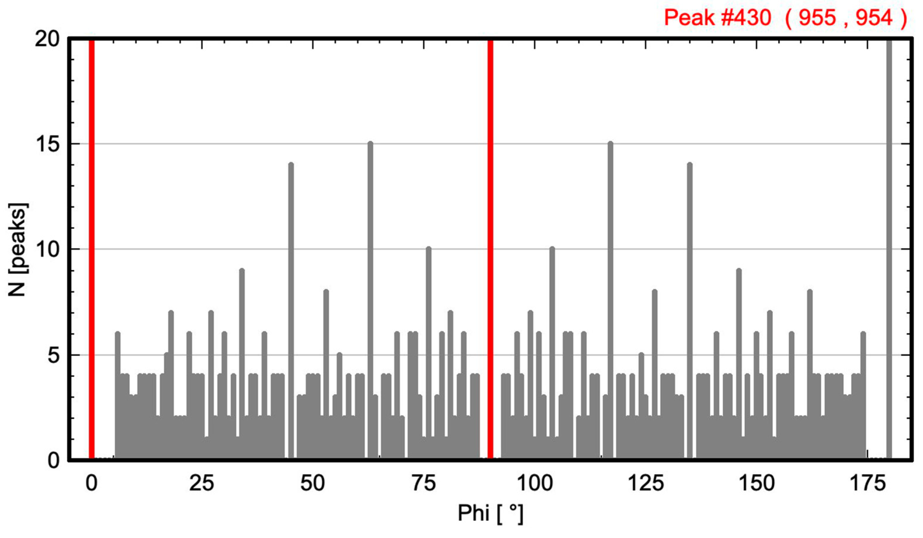
| Maximum Atom Peak Displacement in Pixel | Maximum Atom Peak Displacement in Å | Number of Analyzed Atom Peaks for Barium Within Maximum Circle | 1st Maximum (Red) at Angle | 2nd Considered Maximum (Green) at Angle | Determined Cell Angle from ALPD Plot |
|---|---|---|---|---|---|
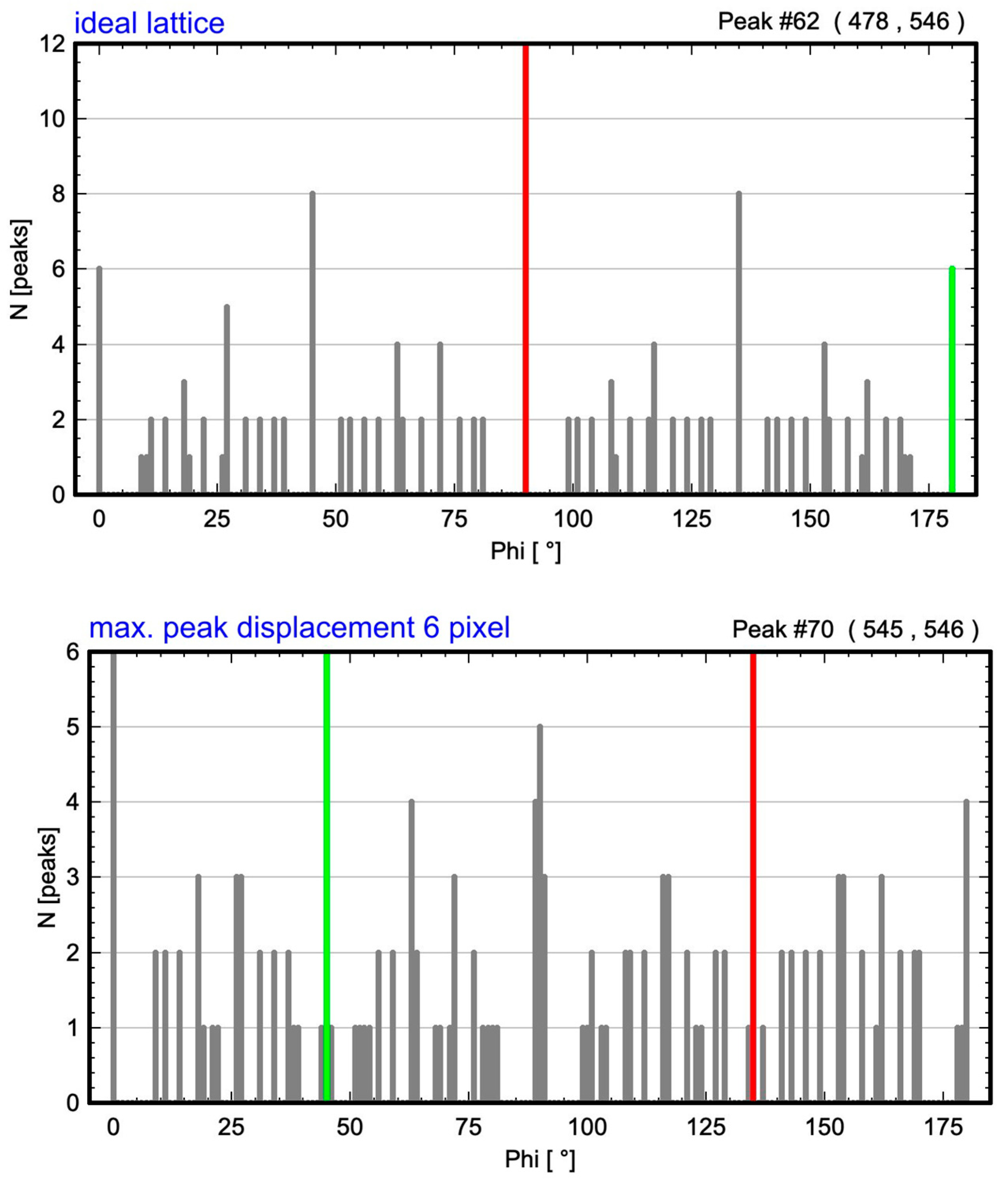
| 0 | 0 | 144 | 90° | 180° | 90° |
| 6 | 0.36 | 144 | 135° | 45° | 90° |
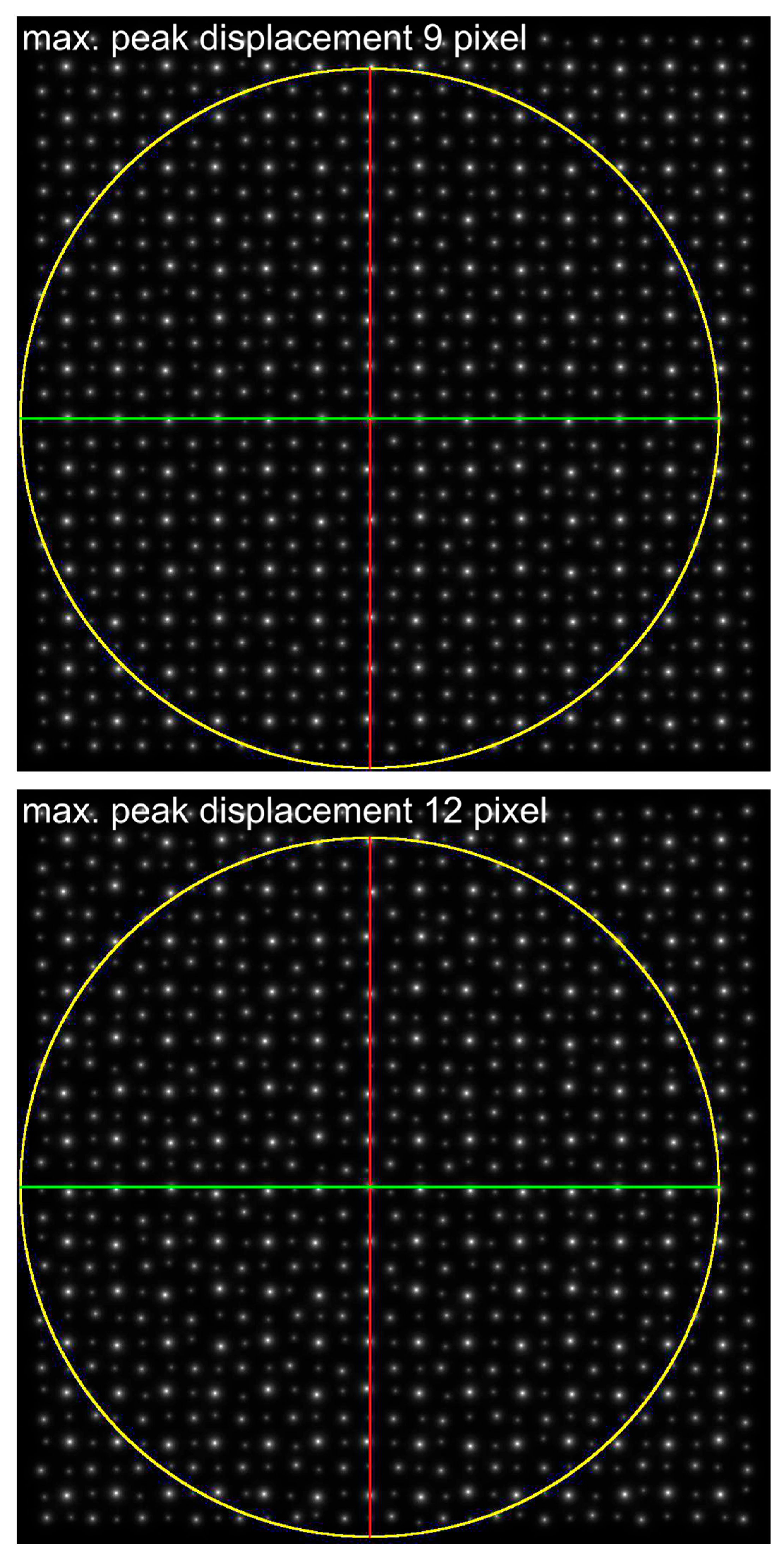
| 9 | 0.53 | 144 | 90° | 0° | 90° |
| 12 | 0.71 | 148 | 90° | 0° | 90° |
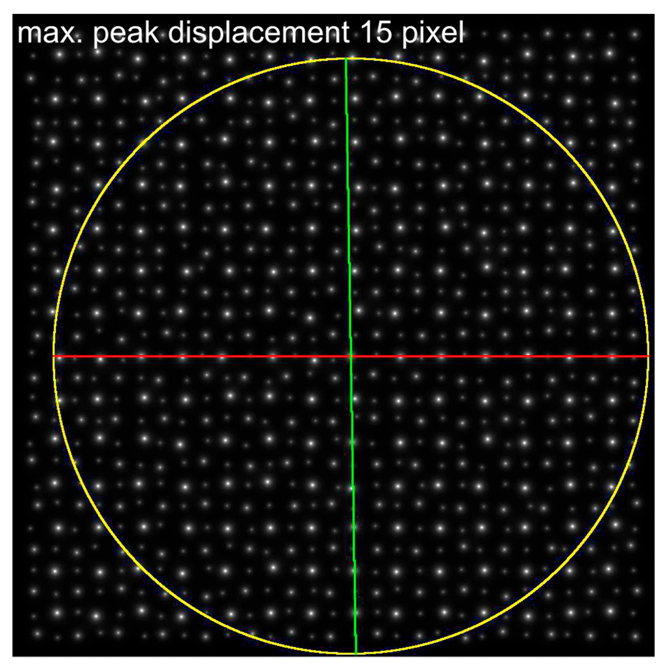
| 15 | 0.89 | 146 | 0° | 89° | 89° |
Disclaimer/Publisher’s Note: The statements, opinions and data contained in all publications are solely those of the individual author(s) and contributor(s) and not of MDPI and/or the editor(s). MDPI and/or the editor(s) disclaim responsibility for any injury to people or property resulting from any ideas, methods, instructions or products referred to in the content. |
© 2025 by the author. Licensee MDPI, Basel, Switzerland. This article is an open access article distributed under the terms and conditions of the Creative Commons Attribution (CC BY) license (https://creativecommons.org/licenses/by/4.0/).
Share and Cite
Weirich, T.E. Angle-Resolved Lattice Population Density Plots: A Novel Approach for Fast 2D Unit Cell Determination from HAADF STEM Images. Symmetry 2025, 17, 239. https://doi.org/10.3390/sym17020239
Weirich TE. Angle-Resolved Lattice Population Density Plots: A Novel Approach for Fast 2D Unit Cell Determination from HAADF STEM Images. Symmetry. 2025; 17(2):239. https://doi.org/10.3390/sym17020239
Chicago/Turabian StyleWeirich, Thomas E. 2025. "Angle-Resolved Lattice Population Density Plots: A Novel Approach for Fast 2D Unit Cell Determination from HAADF STEM Images" Symmetry 17, no. 2: 239. https://doi.org/10.3390/sym17020239
APA StyleWeirich, T. E. (2025). Angle-Resolved Lattice Population Density Plots: A Novel Approach for Fast 2D Unit Cell Determination from HAADF STEM Images. Symmetry, 17(2), 239. https://doi.org/10.3390/sym17020239