Adaptive Invariant Object Representation

Abstract

In this work, one new approach for RSTB-invariant object representation is presented based on the modified Mellin–Fourier Transform (MFT). For this, in the well-known steps of MFT, the logarithm operation in the log-polar transform is replaced by the operation “rising on a power”. As a result, the central part of the processed area is represented by a significantly larger number of points (transform coefficients), which permits us to give a more accurate description of the main part of the object. The symmetrical properties of the complex conjugated transform coefficients were used, and as a result, the number of coefficients participating in the object representation can be halved without deteriorating the quality of the restored image. The invariant representation is particularly suitable when searching for objects in large databases, which comprise different classes of objects. To verify the performance of the algorithm, object search experiments using the K-Nearest Neighbors (KNN) algorithm were performed, which confirmed this idea. As a result of the analysis, it can be concluded that the complexity of the solutions based on the proposed method depends on the applications, and the inclusion of neural networks is suggested. The neural networks have no conflict with the proposed idea and can only support decision making.

1. Introduction

People can successfully perceive and respond to the surrounding world because, throughout their lives, they create, in their minds, abstract representations of perceived objects. These are not just images received through their eyes but a form of generalized related information kept in their minds. As is known, human perception includes five senses: touch, sight, sound, smell, and taste, but the main pieces of information that enter the human brain are through the eyes. The successful survival of individuals in the complex surrounding world depends on their ability to adapt successfully, which depends on their accumulated experience and knowledge. On the basis of this knowledge, a technique is created to recognize complicated objects in complex scenes, called “invariant object recognition”. This is used to identify objects successfully, despite the possible changes in one’s view due to a new position, distance, rotation, and illumination. As a result of accumulated preliminary experience and training, the brain creates its own invariant object representations based on extracted specific features [1,2]. In all such cases, these features can undergo modifications due to environmental conditions [3,4], which implies the taken decision to be adaptive and flexible.

When we try to transfer this knowledge to the field of automation, significant difficulties arise, since the processing and analysis of obtained information is handled depending on the application and specific requirements. In contemporary machine-learning-based approaches, there exist numerous problems, which require corresponding solutions. On the one hand, there are fundamental issues related to the perception of real-world objects that are to be represented digitally. The basic case is when the objects are represented as 2D images, while more complicated problems arise when the objects are 3D, or even multidimensional. Another problem, which attracts significant scientific interest, is related to digital object generation. In this case, contemporary techniques such as text-to-image generative models are involved; for example, [5]. One of the existing limitations is that these models usually consistently generate the same objects in different contexts, with similar appearances. This shortcoming has sure advantages when used to generate comic book illustrations or other similar applications. One more contemporary technique is the creation of large-scale text-to-image models which generate high-quality and diverse images, and this approach has already shown remarkable success. These models are mainly focused on the creation of multi-subject scenes, but they have certain difficulties when generating complex images that involve many objects of various kinds [6,7,8]. A significant part of this research is also aimed at object searches in image databases or in real-life scenes. Such tasks are mainly executed by collaborative robots, who must be capable of finding the needed objects among many others. In many cases, to solve this task, some limitations have to be preliminarily set, such as, for example, reducing the problem from 3D to 2D, selecting a narrower view area, changing the brightness requirements, etc. [9,10].

In all these cases, the successful implementation of the existing complicated tasks highly depends on the used features. As is known, the main question is how to select the minimum number of features that are sufficient for reliable and reasonable decision making (i.e., recognition). An additional requirement is that these features retain their qualities in various positions, color changes, rotations, etc., of the represented objects. In general, starting from the early years of pattern recognition, the methods for object descriptions were divided into two basic groups of features: local and global. To the first group belongs features related to such qualities of the objects, which mainly represent the structure of their visible part [11,12]. A shortcoming of these features is their vulnerability against noises, and together with this, they usually have high dimensionality and need significant computational complexity. To the second group belong features that represent the general qualities of the visible part of the object (geometrical parameters, etc.) [13]. These features have good insensibility to noises, but their computational complexity is also relatively high. Here also belong various kinds of 2D and 3D transformations, whose coefficients are used as global features. These are the Discrete Cosine Transform (DCT), the Walsh–Hadamard Transform (WHT), the Fourier transform, and many others. Each transform has its specific advantages or shortcomings: some of them are more suitable when searching for certain textures, others are used when searching for a given color, and still others have the lowest computational complexity. At the same time, the issue of the invariance of features is gaining more and more importance, since the modern technique has to deal with tasks of very high difficulty in terms of the objects’ shape and the complexity of the analyzed scenes. These problems have attracted the attention of a large number of researchers, and as a result, a significant number of algorithms and methods have already been developed. The basic methods for invariant object representation are related to 2D rigid transforms, i.e., combinations of rotation, scaling, and translation (RST). Accordingly, 2D objects in still images are depicted by descriptors of three basic kinds: shape boundary, region, and color. To the first kind are assigned the chain codes, Fourier descriptors, Generalized Hough Transform, the Active Shape Model, etc. More complicated shapes require the use of highly intelligent and adaptive approaches [14,15,16,17]. Another tool for invariant representation is the histogram descriptor. Its main advantage is the robustness to changes in an object’s rotation, scale, and partial changes in the viewing direction, but it has one big disadvantage—the structural information is lost, which is sometimes unacceptable. One more solution is to use a combination of Discrete Wavelet Transform (DWT) or Discrete Fourier Transform (DFT) in the feature extraction process. One reliable solution is, for the extraction of the rotation–scale–translation (RST), invariant features that use descriptors based on the log-polar transform (LPT) used to convert rotation and scaling into translation [18] and on the 2D Mellin–Fourier Transform (2D-MFT) [19,20]. The basic problem for the creation of the RST-invariant descriptors is the need to calculate a large number of spectrum coefficients, and as a sequence, the high computational complexity.

In this work, one new approach for invariant object representation based on the modified Mellin–Fourier transform with the adaptive selection of the most suitable coefficients is proposed. The obtained descriptors are invariant to 2D rotation (R), scaling (S), translation (T), and brightness (B) changes, i.e., RSTB-invariant.

The structure of this paper is as follows: Section 2 gives the concepts of the modified MFT method for 2D still images; Section 3 gives the symmetry attributes of the RSTB-invariant object representation; Section 4 shows some experimental results and presents the new adaptive architecture for 3D visual information; and Section 5 is the conclusion.

2. RSTB-Invariant Object Representation Based on the Modified MFT

A Mellin–Fourier Transform representation of 2D grayscale digital images.

As is known, the MFT comprises three consecutive steps: DFT, LP Transform, and second DFT. The mathematical presentation of MFT is given below for grayscale images (2D matrices) of size L × W. The transform is executed as follows:

-

The pixels G(l,w) of the original halftone image matrix of size L × W are transformed into bipolar form:

$$\mathrm{T}(\mathrm{l},\mathrm{w})=\mathrm{G}(\mathrm{l},\mathrm{w})-({\mathrm{G}}_{\max } +1)/2$$

(1)

For l = 0, 1, …, L − 1 and w = 0, 1, …, W − 1,

Where G_max is the maximum pixel brightness value in the grayscale image (G_min = 0).

-

The image matrix is processed with 2D Discrete Fourier Transform (2D-DFT), executed in a window of size n × n, which frames the object. In this case, n is an even number. For the invariant object representation, the 2D-DFT coefficients are used and calculated accordingly:

$$\mathrm{F}(\mathrm{u} ,\mathrm{v})={\displaystyle \sum _{\mathrm{l}=0}^{\mathrm{n}-1}{\displaystyle \sum _{\mathrm{w}=0}^{\mathrm{n}-1}\mathrm{T}(\mathrm{l},\mathrm{w}) }}\exp \{-\mathrm{j} \left[\right(2\mathrm{\pi }/\mathrm{n}\left)\right(\mathrm{lu}+\mathrm{w}\mathrm{v})]\}$$

(2)

For $\mathrm{u}=0,1,\dots ,\mathrm{n}-1$ and $\mathrm{v}=0,1,\dots ,\mathrm{n}-1$.

The transform comprises two steps: a one-dimensional transform of the pixels T(w,l), executed consecutively for the matrix rows, and after that for the matrix columns.

After the 1D-Fast Fourier Transform (1D-FFT), for the values $\mathrm{l}=0, 1,\dots ,\mathrm{n}-1$, the coefficients are calculated:

$$\begin{array}{l}\mathrm{F}(\mathrm{l},\mathrm{v})={\displaystyle \sum _{\mathrm{w}=0}^{\mathrm{n}-1}\mathrm{M}(\mathrm{l},\mathrm{w})\exp \{-\mathrm{j} [2\mathrm{\pi }(\mathrm{wv}/\mathrm{n})]\}}=\\ ={\displaystyle \sum _{\mathrm{w}=0}^{\mathrm{n}-1}\mathrm{M}(\mathrm{l},\mathrm{w})\cos [2\mathrm{\pi }(\mathrm{wv}/\mathrm{n})]} -\mathrm{j}{\displaystyle \sum _{\mathrm{w}=0}^{\mathrm{n}-1}\mathrm{M}(\mathrm{l},\mathrm{w})\sin [2\mathrm{\pi }(\mathrm{wv}/\mathrm{n})]}\end{array}$$

(3)

Correspondingly, for $\mathrm{v}=0,1,\dots , \mathrm{n}-1$ after the second 1D-FFT, the coefficients are calculated:

$$\begin{array}{l}\mathrm{F}(\mathrm{u},\mathrm{v})={\displaystyle \sum _{\mathrm{l}=0}^{\mathrm{n}-1}\mathrm{F}(\mathrm{l},\mathrm{v})\exp \{-\mathrm{j} [2\mathrm{\pi }(\mathrm{lu}/\mathrm{n}) ]\}}=\\ ={\displaystyle \sum _{\mathrm{l}=0}^{\mathrm{n}-1}\mathrm{F}(\mathrm{l},\mathrm{v})\cos [2\mathrm{\pi }(\mathrm{lu}/\mathrm{n})]}- \mathrm{j}{\displaystyle \sum _{\mathrm{l}=0}^{\mathrm{n}-1}\mathrm{F}(\mathrm{l},\mathrm{v})\sin [2\mathrm{\pi }(\mathrm{lu}/\mathrm{n})]}={\mathrm{A}}_{\mathrm{F}}(\mathrm{u} ,\mathrm{v})-\mathrm{j} {\mathrm{B}}_{\mathrm{F}}(\mathrm{u} ,\mathrm{v})\end{array}$$

(4)

Here, A_F(u,v) and B_F(u,v) are the real and the imaginary parts of the coefficients’ components.

-

The calculated Fourier coefficients are positioned in the center of the spectrum plane:

$${\mathrm{F}}_0(\mathrm{u},\mathrm{v})=\mathrm{F}(\mathrm{u}-\frac{\mathrm{n}}{2},\mathrm{v}-\frac{\mathrm{n}}{2}),\mathrm{for}\mathrm{u},\mathrm{v}=0,1,\dots ,\mathrm{n}-1$$

(5)

-

Part of the coefficients are retained for further processing in accordance with the conditions:

$${\mathrm{F}}_{0\mathrm{R}}(\mathrm{u} ,\mathrm{v})=\left\{\begin{array}{c}{\mathrm{F}}_0(\mathrm{u},\mathrm{v}),\mathrm{i}\mathrm{f}(\mathrm{u},\mathrm{v})\in \mathrm{r}\mathrm{e}\mathrm{t}\mathrm{a}\mathrm{i}\mathrm{n}\mathrm{e}\mathrm{d} \mathrm{r}\mathrm{e}\mathrm{g}\mathrm{i}\mathrm{o}\mathrm{n};\\ 0 - \mathrm{other} \mathrm{cases}.\end{array}\right.$$

(6)

The retained coefficients are positioned in a square with a side of length Z ≤ n, which envelops the center (0,0) of the spectrum area (Z—even number). For Z < n and $\mathrm{u},\mathrm{v}=- (\mathrm{Z}/2), -(\mathrm{Z}/2)+1,\dots ,-1,0,1,\dots ,(\mathrm{Z}/2)-1$, this square contains the low-frequency coefficients only.

-

The modules and phases of the retained coefficients are calculated and then the modules ${\mathrm{D}}_{{\mathrm{F}}_{0\mathrm{R}} }(\mathrm{u},\mathrm{v})$ of the Fourier coefficients ${\mathrm{F}}_{0\mathrm{R}}(\mathrm{u},\mathrm{v})$ are normalized:

$$\mathrm{D}(\mathrm{u},\mathrm{v})=\mathrm{p}\ln {\mathrm{D}}_{{\mathrm{F}}_{0\mathrm{R}}} (\mathrm{u},\mathrm{v});$$

(7)

p denotes the normalization coefficient.

-

For the coefficients $\mathrm{D}(\mathrm{u},\mathrm{v})$, the log-polar transform is executed, which is performed in such a way that the central point (0,0) of the polar coordinate system $(\mathrm{\eta },\mathrm{\delta })$ coincides with the center of the coefficients’ module area $\mathrm{D}(\mathrm{u},\mathrm{v})$, which is in the rectangular coordinate system. For this, the variables are changed accordingly:

$$\mathrm{\eta }=\log \sqrt{{\mathrm{u}}^2 +{\mathrm{v}}^2},\mathrm{\delta }=\mathrm{arctg}(\mathrm{v}/\mathrm{u})$$

(8)

The values of η and δ are discrete and in the range

$$\mathrm{u},\mathrm{v}=- (\mathrm{Z}/2),\dots ,-1,0,1,\dots ,(\mathrm{Z}/2)-1$$

As a result of the new positioning, part of the coefficients $\mathrm{D}(\mathrm{\eta } ,\mathrm{\delta })$ are missed because the area in which they are positioned is changed. To obtain the needed coefficients, for the missing part of them, new values are calculated. They are obtained after interpolation with the closest neighbors $\mathrm{D}(\mathrm{u} ,\mathrm{v})$ in the rectangular coordinate system $(\mathrm{u} ,\mathrm{v})$, in horizontal and vertical directions, through zero-order interpolation. In this processing step, the main problem is how to arrange the points so that they are positioned evenly in the processed space. For this, a number of discrete circles of points in the polar system are arranged. In this approach presented here, the corresponding radiuses of these circles ρ_i are set to be equal to the number of the discrete angles δ_i for the discrete values of i = 1, 2, …, Z. In the rectangular coordinate system, the side of the square Z, which is inscribed in the LPT matrix, has to be calculated to transfer as many coefficients without change as possible. To achieve this, the radius of the circumscribed circle is calculated accordingly:

$$\mathrm{r}=\mathrm{Z}\sqrt{2}/2$$

(9)

and is set the smallest step (Δη) between each two concentric circles: $\Delta \mathrm{\eta }={\mathrm{r}}^{(1/\mathrm{Z})}$. Then, for each discrete radius η_i and angle δ_i, we obtain the following relations:

$${\mathrm{\eta }}_{\mathrm{i}}={(\Delta \mathrm{\eta })}^{\mathrm{i}}={\mathrm{r}}^{\mathrm{i}/\mathrm{Z}} \mathrm{for}\mathrm{i}=1,2,\dots ,\mathrm{Z};$$

(10)

$${\mathrm{\delta }}_{\mathrm{i}} =(2\mathrm{\pi }/\mathrm{Z}) \mathrm{i}\mathrm{for} \mathrm{i}=(-\mathrm{Z}/2),.,0,.,(-\mathrm{Z}/2)-1$$

(11)

These relations explain the main difference between the well-known log-polar (LP) transform and the new approach: in the LP transform, the mathematical expression used to set the values of the radiuses is based on a logarithmic relation. The new positioning of the selected points shown above is based on the operation “rising on a power”. This is a kind of modified LP transform called the Modified Polar Transform, MPT. As a result of this operation and after interpolating the coefficients of $\mathrm{D}(\mathrm{u} ,\mathrm{v})$, one new matrix is obtained with coefficients D(f,g) for f, g = 0, 1, 2, …, Z − 1.

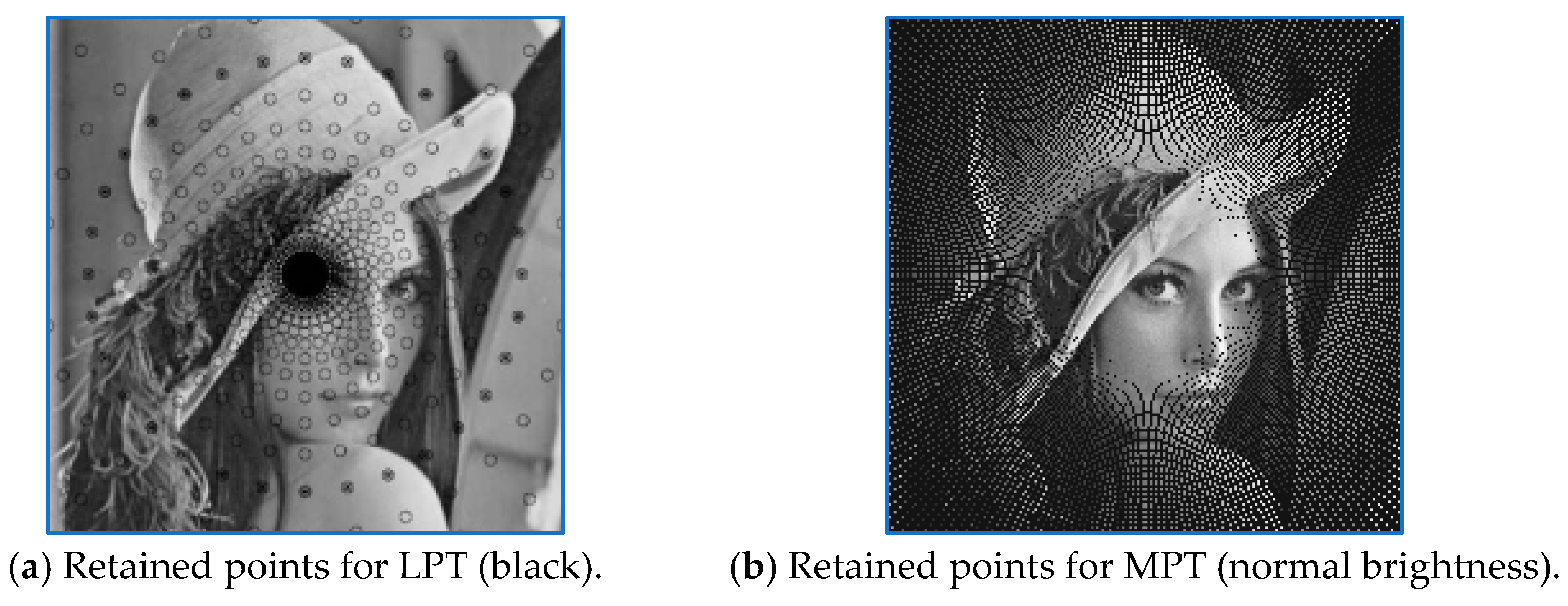
Figure 1 shows the difference between the positioning of the used points in both cases and how the new approach changes the area of the retained part of the object. For both examples, the number of points is the same, but their distribution is different. Figure 1a shows the central part of the test image “Lena” (200 × 200 pixels), which corresponds to the LPT case. The retained points, whose data are used for further processing, are black. Figure 1b shows the same part of the test image for the MPT case. In this figure, the used points are with their original brightness. It is easy to notice that the central part of the processed area for the MPT is significantly expanded, which permits one to obtain a more detailed representation from the points placed in the central part of the image, where the most significant part of the visual information is usually positioned.

Following the steps of MFT, for the matrix D(f,g), the second 2D-DFT is executed, and from Equations (3) and (4), the following is obtained:

$$\mathrm{S}(\mathrm{u} ,\mathrm{v})={\displaystyle \frac{1}{{\mathrm{Z}}^2}} {\displaystyle \sum _{\mathrm{f}=0}^{\mathrm{Z}-1} {\displaystyle \sum _{\mathrm{g}=0}^{\mathrm{Z}-1}{\mathrm{D}}_{\mathrm{I}}(\mathrm{f}, \mathrm{g}) }}\exp \{-\mathrm{j} \left[\right(2\mathrm{\pi }/\mathrm{Z}\left)\right(\mathrm{fu}+\mathrm{g}\mathrm{v})]\}$$

(12)

For $\mathrm{u}=0,\dots ,\mathrm{Z}-1$ and $\mathrm{v}=0,\dots ,\mathrm{Z}-1$.

The modules of the coefficients $\mathrm{S}(\mathrm{u},\mathrm{v})$ are

$${\mathrm{D}}_{\mathrm{S}}(\mathrm{u},\mathrm{v})=\sqrt{{[{\mathrm{A}}_{\mathrm{S}}(\mathrm{u},\mathrm{v})]}^2+{[{\mathrm{B}}_{\mathrm{S}}(\mathrm{u},\mathrm{v})]}^2}.$$

(13)

Here, A_S(u,v) and B_S(u,v) are correspondingly the real and the imaginary component of $\mathrm{S}(\mathrm{u} ,\mathrm{v})$.

This is the last operation of the MFT, and as a result, the RST (rotation–scale–translation)-invariant representation of the object is obtained. An additional possibility is to add invariance towards brightness (B) changes, and for this, the modules of the MFT coefficients are normalized:

$${\mathrm{D}}_{{\mathrm{S}}_0}(\mathrm{u},\mathrm{v})={\mathrm{G}}_{\max } [{\mathrm{D}}_{\mathrm{S}}(\mathrm{u},\mathrm{v})/{\mathrm{D}}_{\mathrm{S}\max }(\mathrm{u},\mathrm{v})],$$

(14)

where ${\mathrm{D}}_{\mathrm{S}\max } (\mathrm{u},\mathrm{v})$ is the coefficient with the maximum value.

As a result, the so-calculated transform coefficients represent the processed object image in RSTB-invariant form.

For the future use of the 2D object invariant representation, the coefficients are transformed into vector form. For this, the vector components are calculated in accordance with the following relations:

$${\Sigma }_1(\mathrm{u})={\displaystyle \sum _{\mathrm{b}=0}^{\mathrm{Z}/2}{\mathrm{D}}_{{\mathrm{S}}_0}(\mathrm{u},\mathrm{v})}$$

(15)

For u = 0, 1,…, (Z/2) – 1 and

$${\Sigma }_2(\mathrm{v})= {\displaystyle \sum _{\mathrm{u}=0}^{\mathrm{Z}/2}{\mathrm{D}}_{{\mathrm{S}}_0}(\mathrm{u},(\mathrm{Z}-1-\mathrm{v}))}$$

(16)

For v = 0, 1, …, (Z/2) − 1.

Then, from Equations (15) and (16), the RSTB-invariant vector of size 1 × H is obtained:

$$\overrightarrow{\mathrm{V}}={[{\Sigma }_1(0),{\Sigma }_1(1),\dots \dots , {\Sigma }_1({\displaystyle \frac{\mathrm{Z}}{2}}-1),{\Sigma }_2(0),{\Sigma }_2(1),\dots ,{\Sigma }_2({\displaystyle \frac{\mathrm{Z}}{2}}-1)]}^{\mathrm{T}},$$

(17)

Which comprises two vectors of size 1 × Z/2:

$${\overrightarrow{\mathrm{V}}}_{\mathrm{a}}={[{\Sigma }_1(0),{\Sigma }_1(1),\dots ,{\Sigma }_1({\displaystyle \frac{\mathrm{Z}}{2}}-1)]}^{\mathrm{T}},$$

(18)

$${\overrightarrow{\mathrm{V}}}_{\mathrm{b}}={[{\Sigma }_2(0),{\Sigma }_2(1),\dots ,{\Sigma }_2({\displaystyle \frac{\mathrm{Z}}{2}}-1)]}^{\mathrm{T}}$$

(19)

For the 3D object representation, the most suitable approach is for the vectors to be replaced by tensors. These are the cases when we have to process sequences of correlated images (video sequences), groups of multi-view images or multispectral images of the same object, etc. Here also belongs the cases when 3D color images have to be analyzed, and the information about the color components is processed together.

On the basis of the so-obtained RSTB-invariant object representation, an adaptive architecture for object search in large databases could be created.

For the detection of closest objects in large image databases (DBs), the minimum Euclidean distance d_E between the corresponding RSTB vectors is used. For each two Z-dimensional vectors ${\overrightarrow{\mathrm{V}}}_{\mathrm{i}}$ and ${\overrightarrow{\mathrm{V}}}_{\mathrm{j}}$, this distance is defined in the following way:

$${\mathrm{d}}_{\mathrm{E}}({\overrightarrow{\mathrm{V}}}_{\mathrm{i}},{\overrightarrow{\mathrm{V}}}_{\mathrm{j}})={\displaystyle \sum _{\mathrm{n}=0}^{\mathrm{Z}-1}[{\mathrm{v}}_{\mathrm{i}}(\mathrm{n})-{\mathrm{v}}_{\mathrm{j}}}(\mathrm{n}){]}^2,$$

(20)

where ${\mathrm{v}}_{\mathrm{i}}(\mathrm{n}),{\mathrm{v}}_{\mathrm{j}}(\mathrm{n})$ are the corresponding components of vectors ${\overrightarrow{\mathrm{V}}}_{\mathrm{i}} \mathrm{a}\mathrm{n}\mathrm{d} {\overrightarrow{\mathrm{V}}}_{\mathrm{j}}$ for $\mathrm{i}\ne \mathrm{j}.$ The image request classification is performed by taking into account the image classes in the DB and their RSTB vectors. The image request is represented by the Z-dimensional RSTB vector,$\overrightarrow{\mathrm{V}}.$ Accordingly, the RSTB vectors are represented as ${\overrightarrow{\mathrm{V}}}_{\mathrm{\alpha }}^{\mathrm{\beta }} \in {\mathrm{C}}_{\mathrm{\beta }}$ for α = 1, 2, …, R and β = 1, 2, …., L. In the corresponding relation, the number of vectors in the DB is denoted as R; L represents the number of classes and ${\mathrm{C}}_{\mathrm{\beta }}$—is used to represent the class of objects. The classification rule is based on the “K-Nearest Neighbours” and “Majority vote” algorithms [21,22,23]:

$$\overrightarrow{\mathrm{V}}\in {\mathrm{C}}_{\mathrm{\beta }}, \mathrm{i}\mathrm{f} {\mathrm{d}}_1 (\overrightarrow{\mathrm{V}}, {\overrightarrow{\mathrm{V}}}_{{\mathrm{\alpha }}_1}^{{\mathrm{\beta }}_1})\le {\mathrm{d}}_2 (\overrightarrow{\mathrm{V}}, {\overrightarrow{\mathrm{V}}}_{{\mathrm{\alpha }}_2}^{{\mathrm{\beta }}_2})\le \dots \dots \le {\mathrm{d}}_{\mathrm{K}} (\overrightarrow{\mathrm{V}}, {\overrightarrow{\mathrm{V}}}_{{\mathrm{\alpha }}_{\mathrm{K}}}^{{\mathrm{\beta }}_{\mathrm{K}}})$$

(21)

where K is an odd number:

-

The values of α_k are in the range [1,R] for k = 1, 2, …, K;

-

The values of β_k are in the range [1,L] for k = 1, 2, …, K.

The class ${\mathrm{C}}_{\mathrm{\beta }}$ of the vector $\overrightarrow{\mathrm{V}}$ is defined by the most frequent value β of the indices β_k of the vectors ${\overrightarrow{\mathrm{V}}}_{{\mathrm{\alpha }}_{\mathrm{k}}}^{{\mathrm{\beta }}_{\mathrm{k}}} .$

3. Symmetry Attributes of the Presented Approach for RSTB-Invariant Object Representation

The presented approach has some specific features that allow us to use only part of the coefficients without degrading the visual quality of the reconstructed image. For this purpose, the distribution of coefficients with maximum values in the spectral region and their symmetry are analyzed. Specific for the transform is that the complex conjugated coefficients from the left and right halves of the transform space with the same values are placed symmetrically. One more specific feature is that the coefficients with the highest values, which carry the main pieces of information, are positioned at the corners of the spectrum area. As a result, the number of coefficients could be reduced by using only half of the coefficients (represented with their real values only) for further processing, and after that, retaining these with maximum values. The number of transform coefficients is defined by the number of inscribed concentric circles and the number of radiuses in the processed area. The positioning is shown in Figure 2.

Figure 3a shows one example test image (a human face) [24,25], and its visualized 2D-MFT spectrum is shown in Figure 3b. Figure 3c shows an example mask (green) which frames the retained coefficients and the corresponding positions of the imaginary parts of the complex conjugated coefficients (blue). The shape of the mask roughly approximates the shape of the area, which contains the 2D-MFT coefficients with maximum energy. The mask corresponds to the symmetrical location of the most significant coefficients in the spatial domain. The parameter α of the mask defines the number of retained coefficients in correspondence with the relation:

$$\mathrm{M}=2{\mathrm{\alpha }}^2+\mathrm{Z}-2\mathrm{\alpha }=2\mathrm{\alpha }(\mathrm{\alpha }-1)+\mathrm{Z}$$

(22)

4. DL-Based Selection of Retained Coefficients

Vector representation is very efficient when 2D images have to be processed. In a similar way, for the representation of 3D or multidimensional images, tensor representations of corresponding order could be used.

Invariant object representation is used in a large number of applications. One possible example is when one object has to be detected in a large database of complicated images. Also, such a representation could be used for artificially generated objects, where not only the form has to be created but also their texture, etc.

The accuracy of the object restoration depends primarily on the number of coefficients involved in its RSTB representation. On the other hand, the accurate representation of a generated or searched object requires one to use a different number of transform coefficients, whose number depends not only on the shape but also on the color, position, lighting, shadows, etc., i.e., a number of views, possible movement, and so on. The invariant representations of generated objects can be adaptive when modern neural networks and learning methods are involved in their creation. The number of needed coefficients defines the structure of the used neural networks, which can be of varying complexity and may consist of different numbers of layers with specific weights. The examples given below illustrate the complexity of the problem.

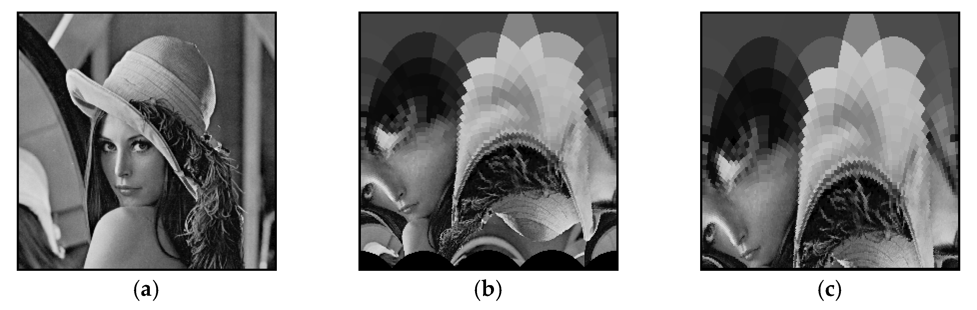
As an example only, Figure 4 shows the intermediate visualized results obtained for the processing of the text image “Lena”. For the experiments, special software was used, developed in the Technical University of Sofia, Windows environment, C++ (Version 6.0 Enterprise). Figure 4a shows the cropped test image used for the experiments (200 × 200 pixels); Figure 4b shows the visualized result after the MPT for vector size 256 and R = 512; Figure 4c shows the vector size and number of radiuses equal to 96; and for Figure 4d, the vector size is 256 and R = 96.

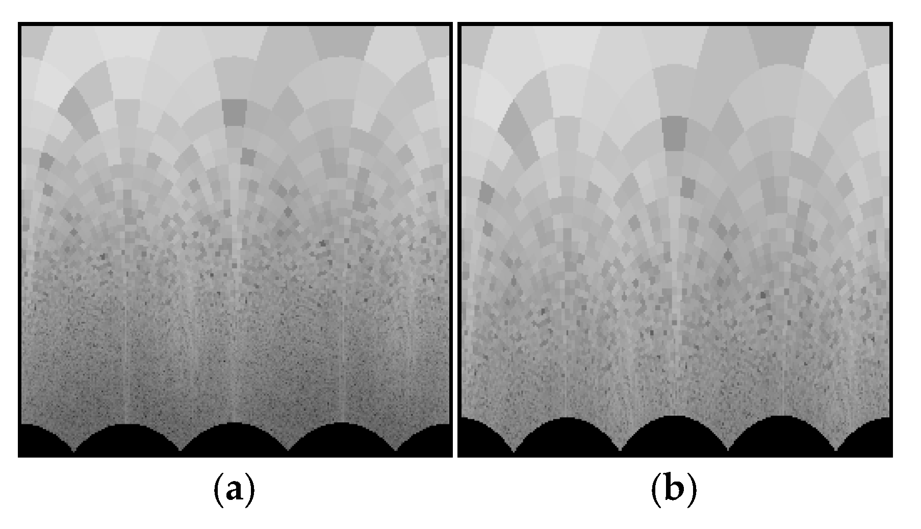
Figure 5 shows the corresponding results for the LPT case.

For comparison only, Figure 6 shows the visualized results obtained for the same vector and radius size when the MPT was used in the transform for the mirror test image “Lena” (rotated at 180 degrees). For these experiments, test images of size 256 × 256 pixels were used. The selection of the vector length for Figure 4 was performed empirically since in this case, the results are used only as an illustration.

Depending on the application, the used number of radiuses and the lengths of the vectors can vary significantly. Together with this, they could be given different weights. One more opportunity is to execute the processing in two or more hierarchical levels, with different numbers of coefficients in each level, which gives, as a result, consecutive approximations of better quality or ensures higher efficiency in decision making when the task, for example, is aimed at object search in large image databases.

Figure 7 shows the block diagram of one example structure which could be used to represent the object into an RSTB vector, to select the most suitable coefficients, and to make a decision about the searched object. The detailed solutions depend on the application. The block diagram is for the 2D case, but it could be transformed without problems for multidimensional tensor representation. Several main applications can be formulated. No specific decision rules are given for Figure 7 because it is only an example of the presented approach. The decision rules change depending on the application. For example, as a decision rule, the PSNR of the restored image could be used compared to the original (in the process of coefficient selection aiming at the best representation, or when a database is created) or the distance between the vector of the image request and these for the images in the database. In all these cases, the size of the mask, the number of radiuses, the length of the vector, etc., could be changed, and the preferred values could be used for decision making.

Example 1. Adaptive object representation.

In this case, the leading conditions are defined by the number of transform coefficients and the visual quality of the restored image of the object. The problem is solved with the compromise between the minimum number of coefficients and the highest possible reproduction quality. For this, the NNs are included in the part related to coefficient selection. For a given class of similar objects, training can be performed in advance, and then the results can be used to create relevant databases in a fast and efficient way.

Example 2. Creation of databases.

In this case, the most important factor is the effective representation of the objects, but the available correlation between the objects should also be analyzed and should be used to further reduce the necessary coefficients or to create classes of objects with a significant visual similarity between them. This variety of solutions, which also influences the structure of the database, requires us to use an increased number of parameters in the process of learning and analysis.

Example 3. Adaptive object search in large databases.

In this case, the decision to detect an object depends on both the efficient choice of coefficients and the algorithm used (for example, K-Nearest Neighbor, etc.). In both cases, it is also possible to use a hierarchical approach with consecutively more accurate approximations. It is important to notice that the image request and the database should be prepared in the same way, i.e., by using the same transform.

In the block diagram, shown in Figure 7, neural networks (NNs) are included in two major positions—in the selection of coefficients, and in the part related to decision making. The type of neural network used depends on the complexity of the task to be solved. If more factors or situations need to be considered, the structure allows for the inclusion of additional steps to aid decision making. The kind of NNs used is not specified here, because the complexity of the preformed task defines the decision rules and the number of analyzed parameters. Besides, the NNs used in the coefficient selection and in the final decision making could be different kinds depending on the task requirements.

The presented approach was used for the creation of an experimental database and corresponding object search for which the results confirmed our idea [26]. A special new format was created for the efficient saving of the coded information, which allows for the addition and expansion of the database with new objects, as well as for the changing of the number of parameters depending on the training and on the specific requirements of the application.

A specific feature of the presented approach is the possibility of using a hierarchical object representation through vectors of different lengths. For this purpose, vectors of relatively small length (for example, up to 256 numbers) are to be used initially, after which the next level is to be created, in which vectors of greater length are to be added.

Based on the presented new approach, some experiments were conducted. For this, we created two databases: one with human faces and the second with groups of multi-view images of the same objects, the purpose of which was to check the effectiveness of our idea. The database with the human faces comprised more than 400 faces—an almost equal number of adults and small children. For the first database, we used 6-10 images of the same person taken at different positions and brightness. For the detection of the closest image in the database, the K-Nearest Neighbor algorithm was used. In all cases, the closest detected object was an image of the same object but rotated or with different brightness. The most important result was that in all cases, without exception, the same object was classified as the closest, regardless of rotation or different lighting. In particular, images rotated on fixed angles (90, 180, or 270 degrees) gave the same values as the representing vector, and naturally, they were defined as “the closest”. The next “closest” were the photos of the same person but with changed brightness or rotated at small angles. These results were confirmed even for small vector lengths (for example, 64 or 96). 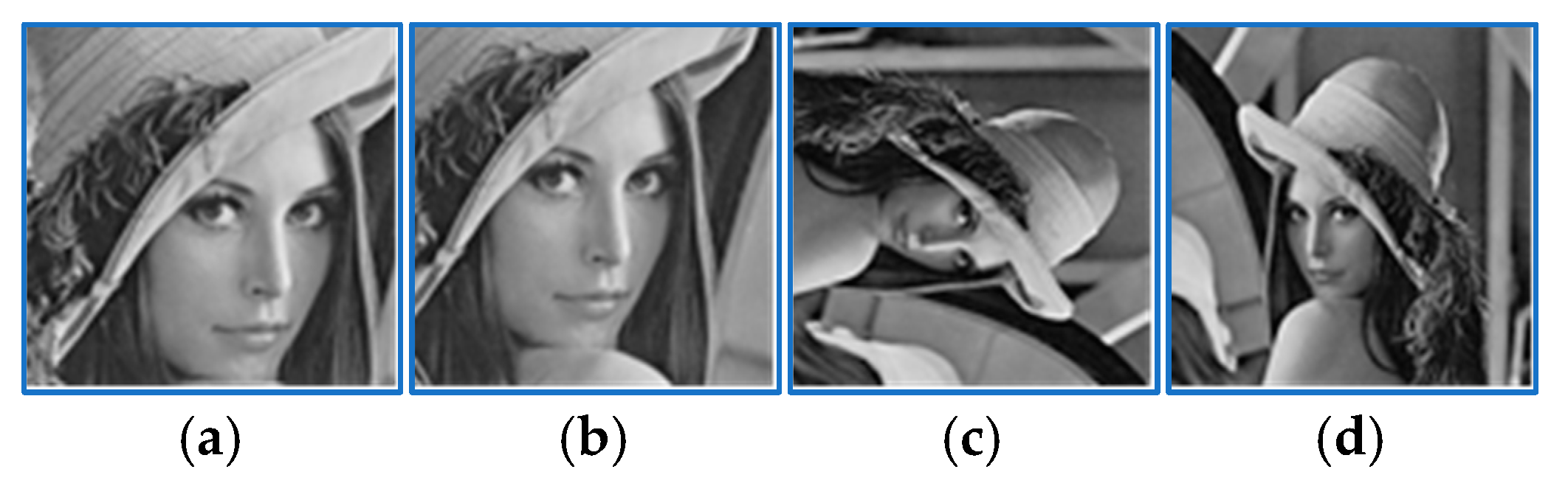Figure 8 shows the results for the closest images obtained for the image request “Lena” in the image database of 400 faces.

The image request is cropped from the original test image “Lenna” (200 × 200 pixels instead of 256 × 256) and is shown as “a”; the closest image detected is denoted as “b”—it is an enlarged version of the image request; the next closest image is denoted as “c” and it is the full original test image rotated 90 degrees; image “d” is the original, rotated 180 degrees; the next closest images are of other persons and are not shown in the figure. The other rotated versions of the original, which are also not shown in the figure, are naturally detected as closer than the remaining images in the database. These experiments are conducted on images from the database, which contains only one class of images, i.e., faces. Figure 9 shows the results for the distance calculated between the corresponding vectors by using the K-NN algorithm. The distances for images 2 and 3 are same because they are only rotated at different angles. The distances to vectors, which represent all other images of faces in the database, are much larger.

The experiments with groups of multi-view images of the same object gave similar results: the rotated images of the image request gave very small differences between the vectors, and the results for all other images were much larger.

In the case that one database contains images, which should be defined as belonging to different classes, the number of needed coefficients increases correspondingly. To better solve this task, in this case, it is suggested to include a neural network, which plays an active part in the selection of parameters and giving them weights. This supports the learning process in the creation of the database and the used object representations. The incorporation of neural networks has no conflicts with the remaining part of the structure and only supports decision making. The structure of the neural network could be selected in accordance with the application and the complexity of the task.

Additional experiments were conducted with a database of scanned documents created at the Technical University of Sofia. It comprised images of texts and signatures (i.e., there are two classes), with more than 100 samples of each class. The scanned documents were examples of texts, written in Latin and Cyrillic alphabets, printed and handwritten, and signatures. All images were of size 256 × 256 pixels and grayscale. For the experiments, two versions of vector generation were used: first version: the size of the retained coefficients square (Z) and the vector length, equal to 96; and second version: the size of the retained coefficients square (Z) and the vector length—equal to 128. Part of the results for the second case are shown in Figure 10.

Figure 10 shows eight of the images in the database. The image request is the upper left and then the next closest, arranged in accordance with the distance calculated between the corresponding vectors. In one of the experiments, the software gives the first 17 closest images. For the case when the vector length was 96, in the last five positions for the first 17 results, five signatures appeared, i.e., they were classified as “texts”. But for the case when the vector length was enlarged up to 128, the first 17 results were correct (i.e., there were only texts). In fact, due to representation scale invariance, the images of signatures in these cases were classified as a kind of large “text”. The results obtained show that for better classification, longer vectors are needed. The presented results for the first 17 images were used only in the process of the method analysis and evaluation. The differences between vectors calculated by using the KNN algorithm are so big after the first 3-5 closest images that for further analysis, only these from the first positions are used. This is why the results after position five are not important and should be neglected.

5. Conclusions

This work presents one new approach for RSTB-invariant object representation, the efficiency of which can be increased when neural networks of different types are included in the process.

The most important feature is that the analysis of the transform coefficients needed for the description of the object permits a significant reduction in their number based on their symmetrical qualities. As a result of the analysis, it was shown that only half of the complex conjugated transform coefficients (the real parts) can be used for the correct representation of the studied object. Besides, an additional reduction in the needed coefficients is also possible using only these, whose values are not negligibly small. To make the correct decision, one could determine which coefficients to be retained for use in the neural networks, which will adds flexibility and adaptability to the presented idea.

The conclusions can be formulated as follows:

• A method for RST-invariant object representation based on a modified MFT transformation is proposed. For this, the log-pol transform, which is a part of the basic MFT, is replaced by a “rising on power” operation. As a result, the central part of the selected area is represented by a larger number of points (coefficients), which ensures a better and more detailed description of the object. Additionally, the new approach is invariant to changes in object brightness, i.e., the representation is RSTB-invariant.
• The symmetrical properties of the transform coefficients were analyzed, and as a result, it was proved that the number of needed coefficients can be halved without deteriorating the quality of the restored image of the object. The analysis shows that the imaginary parts of the complex conjugated coefficient values are not necessary for further processing. For the selection of the retained coefficients, a special spatial “mask” is used, which sets the boundaries of their area depending on the values. The number of the used coefficients can be further reduced after analyzing the magnitude of their values and removing those that are negligibly small.
• The invariant representation is particularly suitable when searching for presegmented objects in large databases which comprise different classes of objects. For this, the specific features of the classes should be defined, and correspondingly, more coefficients should be selected to be used as features. Special research is needed to define the specific features of each class, and here the use of neural networks in the learning process is also suitable.
• The presented approach permits hierarchical representation by using vectors of increasing length.
• The advantage of MMFT over MFT is that the modified version uses rising on power instead of the log-pol Transform, and as a result, the central part of the processed area is represented with a larger number of points. In brief, the advantages of MMFT can be defined in the following way: (a) the number of transform coefficients used for the object representation is significantly reduced, and from this follows the lower computational complexity of the method and (b) the choice of coefficients by selecting a mask used for the vector calculation offers wide possibilities by setting a large number of parameters, each of relatively wide range, which permits the method use in various applications: content- and context-based object retrieval in image databases, etc. With the inclusion of neural networks in the structure of the presented approach, considerable flexibility in decision making is achieved, and after pre-training, the efficiency of the method increases.
• The method could be further developed for multidimensional object representation. In this case, instead of vectors, tensors should be used. In general, the presented approach is quite suitable for such an application and the basic theoretical relations are similar. It is extremely suitable for storage, analysis, and searches for multispectral and multi-view images, sequences of medical information, and many others.

A disadvantage of the method is that it requires prior training in the selection of the most suitable coefficients to be used for the object representation. In the case that similar objects need to be searched for in large databases, vectors of increasing length and complex neural networks are required.

The presented method offers an efficient tool for the representation of multidimensional objects, using the symmetry qualities of the coefficients calculated by using the modified MFT. It is a good basis for further development in various application areas. In the future, our main efforts will be aimed at the tensor-based method implementation for 3D objects.