Abstract
This paper presents a brief survey on the Riemann Hypothesis, a central conjecture in number theory with profound implications, and describes various recent attempts aimed at proving it.
Keywords:
zeros of the Riemann zeta function; the Riemann Hypothesis; sum over all inverse zeta’s nontrivial zeros MSC:
11M06; 11M26
1. Introduction
The Riemann zeta function is usually defined as the Dirichlet series
[1] (Ch. 25), [2] (Ch. I, sec. 1.1, (1.1.1), p. 1), [3] (Ch.1, sec. 1.2, (1), p. 6), which converges for all such that Re, and as its meromorphic continuation in the complex plane, where it has only a simple pole at . It can also be defined by the Euler product formula,
where p runs through all primes, , [2] (Ch. I, sec. 1.1, (1.1.2), p. 1), [3] (sec. 2.1, (1), p. 6).
It is known that vanishes at the infinitely many negative even integers , , called the trivial zeros, as well as at infinitely (countably) many zeros, called nontrivial zeros, located on the “critical line”, Re, a result due to Hardy [3] (Ch. 11, sec. 11.1, p. 226)) [4]. It is not known to date whether other nontrivial zeros exist in , which should necessarily belong to the “critical strip”, . That no such zeros exist is what is called the Riemann Hypothesis (RH, for short).
The importance of the RH rests on its relation with the distribution of primes [3] (Sec. 1.11, p. 22), [5], but also on many equivalent formulations, some quite technical. For some extensive lists, see [6,7,8], for example. There is, in addition, a large number of results whose validity would immediately follow from the validity of the RH.
Indeed, the RH implies, for instance, some strong bound on the growth of the primes counting function, namely sharp estimates on the remainder term in the formulation of the prime number theorem, for which, in 1899, de la Vallée Poussin [9] proved the form
for some positive constant a, where Li is the logarithmic integral. The error term has been ameliorated in the following years. However, it is interesting that some refinements hold assuming the validity of the RH: in 1901, it was shown by Helge von Koch [10] that the RH is equivalent to the more precise estimate
A bound for the constant implied by the symbol was obtained much later by Schoenfeld [11], but again under the validity of the RH.
Many results have been established over the time, the most pertaining to pure mathematics, under the condition that the RH is true. As usual, in coping with difficult unsolved mathematical problems, several collateral results are obtained. Establishing a number of new results may be even more important than achieving the final goal of proving the RH.
To study the zeros of the zeta function, the so-called (Riemann’s) xi function,
 [2] (Ch. II, (2.1.12), p. 16) has also been widely used. For instance, Hardy proved that
  has infinitely (countably) many zeros on the critical line Re [3] (Ch. 11, sec. 11.1, p. 226)) [4].
has infinitely (countably) many zeros on the critical line Re [3] (Ch. 11, sec. 11.1, p. 226)) [4].Numerous properties of general results about the zeta function can be found in a number of books; see [2,3,12], e.g., Several surveys, recording advances and possible paths to prove the RH have appeared regularly in the literature over the time; see, e.g., [12,13,14,15,16]. In particular, it should be emphasized that Titchmarsh’s work, dating back to 1951 [2], is mostly useful for researchers who wish to conduct research on the RH. N. Kurokawa [17], in 2000, provided a significant body of knowledge on the RH for allied zeta-functions, but this work remains relatively unknown, partly due to its being written in Japanese. This list is not intended to be exhaustive.
The literature concerning the RH is vast and constantly growing, with several significant contributions appearing in qualified periodicals in the first half of 2024 alone. Fortunately, unlike in the case of Fermat’s Last Theorem, where any amateur, regardless of his or her incompetence or lack of mathematical background, could naively attempt to tackle the problem, addressing the RH requires a solid understanding of basic mathematics, specifically, knowledge that goes beyond that of a typical sophomore.
It is claimed that some implications of the RH exist also for other fields, such as cryptography and physics. The difficult task of factoring large composite numbers, crucial for some encryption systems, could potentially benefit from a deeper description of prime number distribution. Yet, it is believed that the truth or falsity of the RH has no relevance for the development of factorization methods.
The zeta function and the distribution of primes play also a role in various models met in different branches of physics, such as classical mechanics, statistical physics, and quantum field theory (in particular, in string theory). These relations might even suggest a path towards proving the RH. Mathematics is traditionally seen as supplying the theoretical tools with which physical theories are analyzed. Here this relationship might be reversed, with quantum physics potentially offering new insights into number theory. One proposed strategy for proving the RH is to exploit the Hilbert–Pólya conjecture (see Section 2.2). This requires determining a self-adjoint operator on a Hilbert space, whose eigenvalues would be the ordinates of the zeros of the zeta function. Since this operator is self-adjoint, its eigenvalues must be real. In quantum mechanics, systems are governed by self-adjoint operators, that is, their Hamiltonians. This analogy suggests that perhaps a quantum mechanical system could be found, whose energy levels correspond to the zeros of the zeta function.
The following set of attempts to prove the RH is far from being exhaustive. Typically, they are (recent or less recent) failures.
2. About Some Attempts to Prove the RH
Many attempts aiming either to prove or to disprove the correctness of the RH have been made since the 1859 work of Bernhard Riemann [18], resorting to a variety of methods, some of which somewhat sophisticated.
2.1. Zero-Free Regions
The interesting idea of identifying “zero-free” regions inside the critical strip should be mentioned. Over the years, there has been some interest in determining regions of the shape , for some function tending to infinity as , since this behavior has some relation to the distribution of the prime numbers.
The first of such regions was constructed in 1899 by de la Vallée–Poussin [3] (sec. 5.2, p. 79) [19], but one of the best results has been considered for long time that achieved by Vinogradov and Korobov (see the review paper [19] for references and other cases). For this reason, sometimes these regions are called “Korobov–Vinogradov regions.”
In 2015, Mossinghoff and Trudgian have obtained the largest known zero-free region [20], then further improved in [21]. In [20] the authors showed that no zeros exist in the domain , where , which result improved the previously best-known value , obtained by Jang and Kwon in 2014 [22].
Very recently, in [21] Mossinghoff, Trudgian, and Yang obtained ameliorated explicit zero-free regions. For example, no zeros of the zeta function exist in the Korobov–Vinogradov region
for , and in the classical zero-free region
for . In addition, the authors also obtained the intermediate zero-free region
for , where .
Earlier, in 2006, Freitas [23] established a Li-type criterion (see Section 2.3) to obtain a necessary and sufficient condition for the existence of zero-free strips, contained inside the critical strip, Re. A numerical rigorous result due to Platt and Trudgian belongs to this kind of approach, but this will be reported later, in more detail.
2.2. The Hilbert–Pólya Conjecture
Among the most intriguing ideas proposed to prove the RH, one should perhaps recall the Hilbert–Pólya conjecture, according to which the RH is true because non-trivial zeros of the zeta function correspond (in a certain canonical way) to the eigenvalues of some positive operator. This conjecture has been often regarded as a most promising approach. However, very little is known about its origins; some people attributed its formulation to Hilbert and Pólya, independently, some time in the 1910s.
Andrew Odlyzko had a correspondence with George Pólya between 1981–1982 [24,25], where he asked for a reference, time, and reasoning about this issue. George Pólya replied that he had spent two years in Göttingen, ending around the beginning of 1914, when he tried to learn analytic number theory from Landau. The latter asked him one day: “You know some physics. Do you know a physical reason that the Riemann hypothesis should be true”. This would be the case, he answered, if the nontrivial zeros of the Xi-function were so connected with the physical problem that the Riemann hypothesis would be equivalent to the fact that all the eigenvalues of the physical problem are real. Pólya added that he never published this remark. Incidentally, the aforementioned Xi-function is defined as .
.That is it. It may be too little, too vague, to base some investigations on this, but several researchers, mostly physicists, took it seriously, even though still unsuccessfully.
There are also some theorems by Pólya’s [26,27], [3] (Ch. 12, sec. 12.5, p. 270), that perhaps could be related to the aforementioned plan.
2.3. The Keiper–Li’s Criterion
The Li’s, or better, Keiper–Li’s criterion, concerns the positivity of a certain numerical sequence [28,29,30,31,32]. In 1997, Xian-Jin Li established a necessary and sufficient condition for the validity of the RH, since then known as the “Li’s criterion” [32]; see also [33]. This has the form of a set of inequalities, namely,
the sum being extended to all nontrivial zeros, , of the Riemann zeta function, and understood as in (13) below (Section 3). In [28], the conditions in (8) are formulated with the ’s strictly positive.
In some sense, there are two ways to evaluate the ’s. One is to look at their definition,
 which comes from the representation
 of the xi function (4) [33] (sec. 4, eq. (20), p. 767) [34] (sec. 4.2). Here, the symmetry relation has been used. Other equivalent formulations for the ’s exist; see, e.g., [35], and also [30,36,37]. In several papers [30,35,36], M. Coffey derived an alternative representation of Li’s coefficients and then used it to tabulate the first 25 values of (for ) in [35], and 101 values (for ) in [36]. These alternative coefficients involve other well-known constants, such as the Stieltjes constants and Bernoulli numbers.
has been used. Other equivalent formulations for the ’s exist; see, e.g., [35], and also [30,36,37]. In several papers [30,35,36], M. Coffey derived an alternative representation of Li’s coefficients and then used it to tabulate the first 25 values of (for ) in [35], and 101 values (for ) in [36]. These alternative coefficients involve other well-known constants, such as the Stieltjes constants and Bernoulli numbers.In Figure 1, the behavior of is shown as a function of n, for n up to about 50. Up to , these values are very well fit by a parabola with , then a departure from this behavior is clear [38].
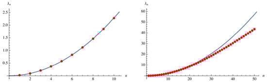
Figure 1.
The coefficients vs. n.
The first 3300 Keiper–Li coefficients were evaluated by K. Maślanka in [39]. A computation for up to n = 100,000, made in [34], shows an agreement on the first two decimals with a certain “Keiper’s conjecture” (hence, with the RH), providing
Keiper’s asymptotic approximation yields in fact [40] (pp. 63–65).
Another way to evaluate the ’s is using the successively obtained Formula (8); see [32]. Using the latter, however, the validity or not of the RH cannot be established since it involves all nontrivial zeros, without knowing whether any of them exist or not off the critical line. In [41], Voros established an alternative asymptotic behavior, basing on (8).
In order to prove (or disprove) the RH via Li’s criterion, one should instead use (9), e.g., which does not involve explicitly the nontrivial zeros themselves. Trying to make explicit the Li’s representation of the parameters , one could use the integral representation of  , given in [35] (eq. (9), p. 527), and consider resorting to the celebrated Faa’ di Bruno formula, which yields the n-th derivative of a given composite function. However, this formula uses sums over set partitions and hence is extremely involved, to the point that to follow this approach seems to be a hopeless task.
, given in [35] (eq. (9), p. 527), and consider resorting to the celebrated Faa’ di Bruno formula, which yields the n-th derivative of a given composite function. However, this formula uses sums over set partitions and hence is extremely involved, to the point that to follow this approach seems to be a hopeless task.2.4. Horizontal Monotonicity
In [42], the so-called “horizontal behavior” of , mentioned by Saidak and Zvengrowski [43], and earlier by Spira [44] was emphasized. It was observed that, at the beginning of the article on the Riemann zeta function, in the Wolfram MathWorld [45], a plot shows horizontal “ridges” of , for and . If indeed such ridges would decrease strictly monotonically for , then the RH would be proved to be true (cf. [43,46]). This behavior is easy to prove outside the critical strip, but nobody has been able to prove it, so far, inside the critical strip.
2.5. Hyperbolicity of Jensen Polynomials
In 1927, G. Pólya proved that the RH is equivalent to the so-called hyperbolicity of Jensen polynomials for the Riemann zeta function at its point of symmetry. This is called the Pólya–Jensen criterion. Advances in this direction are based in the newly discovered fact that these polynomials can be well approximated in terms of Hermite polynomials [47]. This result was initially praised by E. Bombieri [14] as a breakthrough, but this approach was soon considered actually not so useful, hence a not too promising route, by D.W. Farmer [48].
2.6. Basing on New Bounds for Large Values of Dirichlet Polynomials
Very recently, in [49], L. Guth and J. Maynard have posted a significant new result on the arXiv. Largely using Fourier analysis, the authors’ advance towards the Riemann hypothesis rests on improving a result deemed insurmountable for more than 50 years, that is, making the first substantial improvement to a classical 1940 bound of Ingham regarding the zeros of the Riemann zeta function. Field medalist Terence Tao considered this work a remarkable breakthrough. Yet, he still judged it very far from fully proving the RH.
3. Numerical Approach
A continuous progress has been made over the years in computing numerically more and more zeros on the critical line, and exploring the possible existence of zeros off it; see, e.g., [50,51]. Often, computations are based on the Riemann–Siegel formula [52]. Of course, no numerical approach can provide acceptable proofs of the RH, but the numerical path may be useful to formulate conjectures and develop insight. For instance, simulations and visualizations suggest the possible “horizontal monotonicity” of the modulus of , even though, unfortunately, nobody has been able to prove that this occurs inside the critical strip [42].
Relevant computations of the sum of the series
being the nontrivial zeros on the critical line, and estimates (with bounds) for some more general sums were carried out in [53,54]. Some attention has also been devoted to computing the sums , extended over all nontrivial zeros, for fixed k’s, . The ’s are also related to the Li’s coefficients, , defined below; see [33] (eq. (27), p. 768), e.g.
Here are a few examples. In 1982, R.P. Brent et al. have tested the RH computationally, and confirmed its validity for the first 200,000,001 zeros [55]. Such zeros are all located in the critical strip (and lie on the critical line), up to the ordinate t = 81,702,130.19. In 2002, S. Wedeniwski has shown that the first nontrivial zeros lie on the critical line [56]. In [57], it is recalled that in 2004 X. Gourdon [58] used a fast method, developed by Odlyzko and Schoenhage, to verify that the first nontrivial zeros of the zeta function lie on the critical line, which fact validates the RH up to about the ordinate , in the critical strip; see [59]. Actually, A.M. Odlyzko in [51,60] showed the heights of the zeros of the Riemann zeta function numbered up to .
More precisely, in 1988, Odlyzko and Schoenhage developed a fast algorithm for evaluating the Riemann zeta function at many points, using the Fast Fourier Transform [61]. This algorithm reduces the number of operations required to evaluate a finite Dirichlet series of length N at equally spaced values from to . Such a method would enable testing the RH for the first n zeros in operations, as opposed to operations required by earlier methods, provided that no multiple zeros or closely spaced zeros of the zeta function occur.
Later, in 2001 Odlyzko computed the first 10 billion zeros of the Riemann zeta function near height , thus verifying the RH for these zeros and providing further evidence for other conjectures related to the distribution of zeros of the Riemann zeta function [60].
In his 2004 paper, Gourdon presented an optimization of the Odlyzko–Schoenhage algorithm [58]. This efficiently computes the Riemann zeta function at large heights on the critical line and facilitates the computation of zeros of the zeta function through its implementation. He was able to compute two billion zeros from the 1024-th zero of the Riemann Zeta function.
More recently, in 2021, Platt and Trudgian established a remarkable result, verifying that the RH is true up to the height , in a rigorous way, using interval arithmetic [62]. In this way, numerical results can provide proofs.
As it is well known, in order to prove the RH, it suffices to show that no zero of the zeta function exists in the semi-infinite open critical upper half-strip, . In fact, if a nontrivial zero, say , exists in , then also its conjugate, , would be a zero (since is meromorphic and real on the real line), as well as its symmetric one with respect to the critical line Re, that is , and thus as well. This follows from the functional equation obeyed by the zeta function,
[2] (Ch. II, (2.1.1), p. 13), [3] (eq. (4), p. 13), also written, changing s into , [2] (Ch. II, (2.1.8), p. 16).
It follows that nontrivial zeros would come in groups of four if they exist in the critical strip, off the critical line, and in pairs if they are on the critical line. Therefore, if with and is a zero, the Weierstrass factorization of the entire function would contain terms like
where would be the multiplicity of .
would contain terms likeOn the other hand, it is common knowledge too that no zeros exist on the intersection of the critical strip and the real line, as well as on the lines Re, Re. One can thus confine the discussion to the set H, but this region can be restricted further. In fact, it is also known that no nontrivial zero exists in H with an ordinate less than some value. For instance, in [63] (Ex. 10.2.1, (c), p. 353) it is recorded that, if is a nontrivial zero with , then .
However, as mentioned above, in a recent paper, Platt and Trudgian have shown numerically, yet rigorously, using interval arithmetic, that the RH is true up to about the height (cf. [58,59]), that is, all zeros existing in the critical strip, with imaginary part , have real part Re (and are all simple), [62]. Consequently, any investigation aimed at ruling out the existence of nontrivial zeros can be confined just to the set , for some , that can be taken equal to . Considering the shape of the known zero-free regions, we can state that any hypothetical nontrivial zero should be located in such set and very close to and at the right of the vertical line Re, or very close to and at the left of the vertical line Re (or symmetrically, of course, both with respect the line Re and to the real line).
That no nontrivial zeros exist off the critical line, below some value of t can also be shown aby pplying the well-known equation for the sum of the inverse nontrivial zeta’s zeros,
where the sum is extended over all nontrivial zeros of the zeta function, and is the Euler–Mascheroni constant. This equation was already known to Riemann [3] (Ch. 3, sec. 3.8, p. 67, eq. (4)), and appears also in Li’s criterion [28,31,32]. The sum on the left-hand side of (12) does not converge absolutely, but each term is intended to be grouped with its conjugate [64] (Ch. 12, p. 81), [65] (p. 214), and the sum is understood as
termed “*-convergence” by Bombieri and Lagarias [who also used the unusual notation to denote chopping off further decimals of x] [28] (p. 275). As already recalled, each nontrivial zero is necessarily accompanied by its complex conjugate as well as by its symmetric one with respect to the critical line (if it lies off this line), and thus by the conjugate of the latter too. Therefore, as we stated above, if a nontrivial zero, say , exists in the critical strip, off the critical line, with , , then also , , and will contribute to the sum on the left-hand side of (12) with the amount
For the last inequality, the result of [63] (Ex. 10.2, 8. (a), p. 355) was used. This estimate is useful to rule out that some might be a nontrivial zero.
In fact, if we define the following sums of the inverses of zeros:
- : when extended to all nontrivial zeros (including both those on the critical line and those off the critical line, if any exist), see Equation (12);
- : when extended only to all nontrivial zeros located on the critical line;
- : when extended only to all nontrivial zeros off the critical line;
- : when extended only to the first 200 nontrivial zeros located on the critical line (note that each zero with is included along with its conjugate),
then we have
since does not include all nontrivial zeros lying on the critical line, and represents the contribution of a single nontrivial zero located off the critical line (along with its complex conjugate, its symmetrical counterpart, and the conjugate of the symmetrical counterpart). Since
by (12), and
as reported in [66] (p. 249), it follows that
which implies the approximate bound
That is, if a nontrivial zero like exists off the critical line, then, necessarily, must be larger than roughly . No such zero can exist below this ordinate.
Of course, significantly larger lower bounds are known to exist: recall for instance, the various results on zero-free regions or the Platt and Trudgian bound of .
4. Summary
It has long been known that all nontrivial zeros of the Riemann zeta function must lie within the open critical strip . Although the existence of infinitely (countably) many zeros on the critical line, Re, has been known since 1914, no proof of the existence or nonexistence of other nontrivial zeros within has been found to date. The Riemann Hypothesis (RH) states that no such other nontrivial zeros exist. This short survey describes a few more or less recent attempts to prove the RH.
Funding
This research received no external funding.
Acknowledgments
The author expresses gratitude to Richard Brent, David Platt, Timothy Trudgian, Purusottum Rath, and Sanoli Gun for valuable private communications. This work was conducted within the framework of the Italian GNFM-INdAM.
Conflicts of Interest
The author declares no conflicts of interest.
References
- NIST Digital Library of Mathematical Functions. Available online: https://dlmf.nist.gov/ (accessed on 23 December 2024).
- Titchmarsh, E.C. The Theory of the Riemann Zeta-Function, 2nd ed.; Heath-Brown, D.R., Ed.; Clarendon Press: Oxford, UK, 1986. [Google Scholar]
- Edwards, H.M. Riemann’s Zeta Function; Academic Press: New York, NY, USA, 1974. [Google Scholar]
- Hardy, G.H. Sur les zéros de la fonction ξ(s) de Riemann. C. R. Acad. Sci. Paris 1914, 158, 1012–1014. [Google Scholar]
- Jameson, G.J.O. The Prime Number Theorem; First Published: 2003; Cambridge University Press: Cambridge, UK, 2004. [Google Scholar]
- The Riemann Hypothesis. Available online: https://www.aimath.org/WWN/rh/rh.pdf (accessed on 23 December 2024).
- Number theory and physics archive. Available online: https://empslocal.ex.ac.uk/people/staff/mrwatkin/zeta/physics.htm (accessed on 23 December 2024).
- Riemann hypothesis. Available online: https://en.wikipedia.org/wiki/Riemann_hypothesis (accessed on 23 December 2024).
- de la Vallée Poussin, C.-J. Sur la fonction ζ(s) de Riemann et le nombre des nombres premiers inférieurs a une limite donnée. Mémoires Couronnés l’Académie Belg. 1899, 59, 1–74. [Google Scholar]
- von Koch, H. Sur la distribution des nombres premiers [On the distribution of prime numbers]. Acta Math. 1901, 24, 159–182. [Google Scholar] [CrossRef]
- Schoenfeld, L. Sharper bounds for the Chebyshev functions θ(x) and ψ(x), II. Math. Comp. 1976, 30, 337–360. [Google Scholar] [CrossRef]
- Borwein, P.; Choi, S.; Rooney, B.; Weirathmueller, A. The Riemann Hypothesis: A Resource for the Afficionado and Virtuoso Alike; Spring, CMS Books in Mathematics; Springer: Berlin, Germany, 2007; ISBN 978-0-387-72125-5. [Google Scholar] [CrossRef]
- Bombieri, E. The classical theory of zeta and L-functions. Milan J. Math. 2010, 78, 11–59. [Google Scholar] [CrossRef]
- Bombieri, E. New progress on the zeta function: From old conjectures to a major breakthrough. Proc. Natl. Acad. Sci. USA 2019, 116, 11085–11086. [Google Scholar] [CrossRef]
- Conrey, J.B. The Riemann Hypothesis. Notices Am. Math. Soc. 2003, 50, 341–353. [Google Scholar]
- Sarnak, P. Problems of the Millennium: The Riemann Hypothesis. 2004. Available online: https://www.claymath.org/library/annual_report/ar2004/04report_sarnak.pdf (accessed on 23 December 2024).
- Kurokawa, N. The 15 years of the Riemann Hypothesis; Iwanami-Shoten: Tokyo, Japan, 2000. (In Japanese) [Google Scholar]
- Riemann, B. Ueber die Anzahl der Primzahlen unter einer gegebenen Grösse. Monatsberichte Berl. Akad. 1859, 2, 2. [Google Scholar]
- Ford, K. Zero-free regions for the Riemann zeta function. In Number Theory for the Millennium, II (Urbana, IL, 2000); A.K. Peters: Natick, MA, USA, 2002; pp. 25–56. [Google Scholar]
- Mossinghoff, M.J.; Trudgian, T.S. Nonnegative trigonometric polynomials and a zero-free region for the Riemann zeta-function. J. Number Theory 2015, 157, 329–349. [Google Scholar] [CrossRef]
- Mossinghoff, M.J.; Trudgian, T.S.; Andrew Yang, A. Explicit zero-free regions for the Riemann zeta-function. Res. Number Theory 2024, 10, 11. [Google Scholar] [CrossRef]
- Jang, W.J.; Kwon, S.H. A note on Kadiri’s explicit zero free region for Riemann zeta function. J. Korean Math. Soc. 2014, 51, 1291–1304. [Google Scholar] [CrossRef]
- Freitas, P. A Li-type criterion for zero-free half-planes of Riemann’s zeta function. J. Lond. Math. Soc. 2006, 73, 399–414. [Google Scholar] [CrossRef]
- Andrew Odlyzko: Tables of zeros of the Riemann zeta function. Available online: https://www-users.cse.umn.edu/~odlyzko/zeta_tables/index.html (accessed on 23 December 2024).
- Hilbert–Pólya conjecture. Available online: https://en.wikipedia.org/wiki/Hilbert%E2%80%93P%C3%B3lya_conjecture (accessed on 23 December 2024).
- Pólya, G. Über die Nullstellen gewisser ganzer Funktionen. Math. Z. 1918, 2, 352–383. [Google Scholar] [CrossRef]
- Pólya, G. Über trigonometrische Integrale mit nur reellen Nullstellen. J. Reine Angew. Math. 1927, 158, 6–18. [Google Scholar] [CrossRef]
- Bombieri, E.; Lagarias, J. Complements to Li’s criterion for the Riemann hypothesis. J. Number Theory 1999, 77, 274–287. [Google Scholar] [CrossRef]
- Brown, F. Li’s criterion and zero-free regions of L-functions. J. Number Theory 2005, 111, 1–32. [Google Scholar] [CrossRef]
- Coffey, M.W. Toward verification of the Riemann hypothesis: Application of the Li criterion. Math. Phys. Anal. Geom. 2005, 8, 211–255. [Google Scholar] [CrossRef][Green Version]
- Gun, S.; Murty, M.R.; Rath, P. Transcendental sums related to the zeros of zeta functions. Mathematika 2018, 64, 875–897. [Google Scholar] [CrossRef]
- Li, X.-J. The positivity of a sequence of numbers and the Riemann hypothesis. J. Number Theory 1997, 65, 325–333. [Google Scholar] [CrossRef]
- Keiper, J.B. Power series expansions of Riemann’s ξ function. Math. Comp. 1992, 58, 765–773. [Google Scholar]
- Johansson, F. Rigorous high-precision computation of the Hurwitz zeta function and its derivatives. Numer. Algorithms 2015, 69, 253–270. [Google Scholar] [CrossRef]
- Coffey, M.W. Relations and positivity results for the derivatives of the Riemann ξ function. J. Comput. Appl. Math. 2004, 166, 525–534. [Google Scholar] [CrossRef][Green Version]
- Coffey, M.W. New results concerning power series expansions of the Riemann xi function and the Li/Keiper constants. Proc. R. Soc. Lond. Ser. A Math. Phys. Eng. Sci. 2008, 464, 711–731. [Google Scholar] [CrossRef]
- Matiyasevich, Y.V. A relationship between certain sums over trivial and nontrivial zeros of the Riemann zeta-function. Math. Notes Acad. Sci. USSR 1989, 45, 131–135. [Google Scholar] [CrossRef]
- Wolfram MathWorld. Available online: https://mathworld.wolfram.com/LisCriterion.html (accessed on 23 December 2024).
- Maślanka, K. Li’s criterion for the Riemann hypothesis–numerical approach. Opusc. Math. 2004, 24, 103–114. [Google Scholar]
- Johansson, F. Fast and Rigorous Computation of Special Functions to High Precision. Ph.D. Thesis, Johannes Kepler Universität, Linz, Austria, 2014. [Google Scholar]
- Voros, A. Sharpening of Li’s criterion for the Riemann hypothesis. Math. Phys. Anal. Geom. 2006, 9, 53–63. [Google Scholar] [CrossRef]
- Matiyasevich, Y.; Saidak, F.; Zvengrowski, P. Horizontal monotonicity of the modulus of the zeta function, the L-function, and related functions. Acta Arith. 2014, 166, 189–200. [Google Scholar] [CrossRef]
- Saidak, F.; Zvengrowski, P. On the modulus of the Riemann zeta function in the critical strip. Math. Slovaca 2003, 53, 145–172. [Google Scholar]
- Spira, R. An inequality for the Riemann zeta-function. Duke Math. J. 1965, 32, 247–250. [Google Scholar] [CrossRef]
- Wolfram MathWorld. Available online: http://mathworld.wolfram.com/RiemannZetaFunction.html (accessed on 23 December 2024).
- Borwein, J.; Bailey, D. Mathematics by Experiment–Plausible Reasoning in the Twenty-First Century; A.K. Peters: Wellesley, MA, USA, 2003. [Google Scholar]
- Griffin, M.; Ono, K.; Rolen, L.; Zagier, D. Jensen polynomials for the Riemann zeta function and other sequences. Proc. Natl. Acad. Sci. USA 2019, 116, 11103–11110. [Google Scholar] [CrossRef]
- Farmer, D.W. Jensen polynomials are not a plausible route to proving the Riemann Hypothesis. Adv. Math. 2022, 411, 108781. [Google Scholar] [CrossRef]
- Guth, L.; Maynard, J. New large value estimates for Dirichlet polynomials. arXiv 2024, arXiv:2405.20552v1. [Google Scholar]
- LMFDB, Database of L-Functions, Modular Forms, and Related Objects. Available online: https://www.lmfdb.org/zeros/zeta/ (accessed on 23 December 2024).
- Odlyzko, A. Tables of Zeros of the Riemann Zeta Function. Available online: http://www.dtc.umn.edu/~odlyzko/zeta_tables/index.html (accessed on 23 December 2024).
- Siegel, C.L. Über Riemanns Nachlaßzur analytischen Zahlen-theorie. Quellen Studien Geschichte Math. Astr. Phys. 1932, 2, 45–80. [Google Scholar]
- Brent, R.P.; Platt, D.J.; Trudgian, T. Accurate estimation of sums over zeros of the Riemann zeta-function. Math. Comp. 2021, 90, 2923–2935. [Google Scholar] [CrossRef]
- Mossinghoff, M.J.; Trudgian, T.S. Oscillations in the Goldbach conjecture. J. Théor. Nombres Bordeaux 2022, 34, 295–307. [Google Scholar] [CrossRef]
- Brent, R.P.; van de Lune, J.; te Riele, H.J.J.; Winter, D.T. On the zeros of the Riemann zeta function in the critical strip. II. Math. Comp. 1982, 39, 681–688. [Google Scholar] [CrossRef]
- ZetaGrid Homepage. Available online: http://www.zetagrid.net/ (accessed on 23 December 2024).
- Voros, A. Discretized Keiper/Li approach to the Riemann hypothesis. Exp. Math. 2020, 29, 452–469. [Google Scholar] [CrossRef]
- Gourdon, X. The 1013 First Zeros of the Riemann Zeta Function, and Zeros Computation at Very Large Height, Preprint. 2004. Available online: http://numbers.computation.free.fr/Constants/Miscellaneous/zetazeros1e13-1e24.pdf (accessed on 23 December 2024).
- Goodman, L.; Weisstein, E.W. “Riemann Hypothesis.” From MathWorld—A Wolfram Web Resource. Available online: https://mathworld.wolfram.com/RiemannHypothesis.html (accessed on 23 December 2024).
- Odlyzko, A.M. The 1022-nd zero of the Riemann zeta function. Dynamical, spectral, and arithmetic zeta functions (San Antonio, TX, 1999), pp. 139–144. Contemp. Math. 2001, 290. [Google Scholar]
- Odlyzko, A.M.; Schönhage, A. Fast algorithms for multiple evaluations of the Riemann zeta function. Trans. Amer. Math. Soc. 1988, 309, 797–809. [Google Scholar] [CrossRef]
- Platt, D.; Trudgian, T. The Riemann hypothesis is true up to 3·1012. Bull. Lond. Math. Soc. 2021, 53, 792–797. [Google Scholar] [CrossRef]
- Montgomery, H.L.; Vaughan, R.C. Multiplicative Number Theory: I. Classical Theory; first ed.: 1967; Cambridge University Press: New York, NY, USA, 2006. [Google Scholar]
- Davenport, H. Multiplicative Number Theory, 2nd ed.; Springer: Berlin/Heidelberg, Germany, 1980. [Google Scholar]
- Bach, E.; Shallit, J. Algorithmic Number Theory, Vol. I: Efficient Algorithms; The MIT Press: Cambridge, MA, USA; London, UK, 1996. [Google Scholar]
- Borwein, J.M.; Bradley, D.M.; Crandall, R.E. Computational strategies for the Riemann zeta function. J. Comput. Appl. Math. 2000, 121, 247–296. [Google Scholar] [CrossRef]
Disclaimer/Publisher’s Note: The statements, opinions and data contained in all publications are solely those of the individual author(s) and contributor(s) and not of MDPI and/or the editor(s). MDPI and/or the editor(s) disclaim responsibility for any injury to people or property resulting from any ideas, methods, instructions or products referred to in the content. |
© 2025 by the author. Licensee MDPI, Basel, Switzerland. This article is an open access article distributed under the terms and conditions of the Creative Commons Attribution (CC BY) license (https://creativecommons.org/licenses/by/4.0/).