Adaptive Terrain Modeling for Side-Slope Surfaces

Abstract

Three-dimensional site modeling is an important aspect of Building Information Modeling (BIM), especially in mountainous areas. Accurate site modeling is essential for efficient construction planning and resource allocation. A key issue in site modeling is how to accurately calculate the shape of side-slopes. It involves three sub-problems: geometric representation of side-slopes, determination of fill/cut types, and intersection of side-slopes surface with the terrain surface. To address this, a two-stage method for constructing side-slope models adaptive to terrain is proposed. In the first stage, a marching algorithm along polylines is used to calculate the intersection points of the site boundary polylines with the terrain surface. These intersection points are used to segment the boundary polylines. A rule-based approach is then applied to automatically determine the fill/cut type for each segment. Subsequently, the equations of the side-slopes passing through each segment are derived using geometric principles. In the second stage, a marching algorithm along the plane is used to trace the intersection lines of side-slopes with the terrain. Finally, the side-slopes are rendered with precision by integrating the equations of each segment with the determined intersection lines. The effectiveness of the method is verified through illustrative examples. Algorithm efficiency analysis and 3D modeling illustrations have demonstrated that this method not only boasts accuracy and swift computation but also excels in the level of automation achieved in the modeling process.

1. Introduction

In the design of sites and roads, side-slopes play a crucial role [1]. They are not only components that connect the original terrain but also determine the scope of the project’s impact on the terrain, as well as the volume of earthwork involved [2,3]. In the actual environment, the terrain often exhibits undulations, and the width of the side-slope will change accordingly. Therefore, accurately calculating the intersection of the side-slope with the terrain is a key issue in side-slope modeling. To address this problem, the common method is to perform transverse sampling along the route, then calculate the characteristic points of the side-slope line in the cross-section (including turning points and intersection points with the terrain) and connect the characteristic points of two cross-sections in sequence to build a three-dimensional model of the side-slope. For example, Civil 3D [4] uses sample lines to obtain terrain cross-sections, then adds the designed road template to the cross-section, and calculates the side-slope toe. By generating side-slope characteristic lines through cross-sections, a corridor is created based on these lines. Similarly, software such as OpenRoads Designer [5] and HintCAD [6] also use this method. The advantages of this method are its simplicity in calculation and the ability to add various components in the cross-section using templates, such as ditches. However, this method also has some disadvantages: ① its calculation accuracy is affected by the spacing of the sampling lines; ② the sampling range must be set in advance and cannot be dynamically changed. One way to overcome these shortcomings is to not use cross-sectional sampling but to directly construct a three-dimensional side-slope surface model and calculate the intersection of the side-slope surface with the terrain surface. To the best of the authors’ knowledge, there is currently no related research discussing this method. The reason may be that the equation of the side-slope surface is a high-order parametric equation, making it difficult to directly calculate its intersection with the triangular mesh surface.

The goal of this study is to automatically generate a side-slope surface that adapts to the terrain along a given three-dimensional polyline and a terrain surface. This task is divided into three sub-problems: the surface expression of the side-slope, the determination of the excavation and filling types, and the intersection of the side-slope with the original terrain. For the first problem, since the side-slope has the same gradient everywhere, the side-slope surface is a constant gradient surface passing through the given spatial curve. The shape of the spatial curve determines the shape of the side-slope surface, and when the line type of the spatial curve is complex (such as the clothoid used in highway transition curves), the side-slope surface equation becomes complex [7,8,9]. For the second problem, we need to automatically divide the filling section, excavation section, and non-filling and non-excavation section along the spatial curve based on the geometric conditions of the excavation and filling changes, using the given spatial curve and terrain surface. Currently, no research literature has been found on this aspect. Finally, for the third problem, that is, the intersection problem between the surface and the triangular mesh, a large number of studies have discussed it, and the methods are mainly divided into two categories [10]: the subdivision method and the marching method. The former [11,12,13] uses the spatial position relationship to find the triangular faces to be intersected from the two surfaces, and the intersection line between the surfaces is formed by connecting the intersection line segments of the triangular faces. The latter [14,15,16] finds the first intersection point and then, starting from this intersection point, uses the topological continuity of the intersection line to track until the entire intersection line is formed.

We propose a two-stage method to solve these problems: the first stage is to automatically determine the excavation and filling types of the side-slope surface along the site boundary line and calculate the equations of each side-slope surface segment; the second stage is to calculate the intersection of each side-slope surface with the terrain triangular mesh. In both stages, an intersection algorithm based on marching tracking is used. In the first stage, we use a line marching algorithm, while in the second stage, we use a surface marching algorithm.

The rest of this paper is organized as follows. First, the side-slope surface equation is derived, and the terrain triangular mesh expression of the half-edge data structure is introduced, see Section 2. Then, we propose a two-stage method. In the first stage, the automatic judgment rules for the excavation and filling types of the side-slope surface are derived, and the side-slope surface group equations are determined, see Section 3. In the second stage, the intersection of the side-slope surface group with the triangular mesh terrain is calculated, see Section 4. Then, we create a site model instance using the two-stage method and analyze and compare the performance of this method, see Section 5. Finally, there is the conclusion section.

2. Geometric Expression

This study involves the representation of two geometric objects. One is the side-slope, which is a plane with a fixed gradient. The other is the terrain surface, which is expressed using triangle meshes.

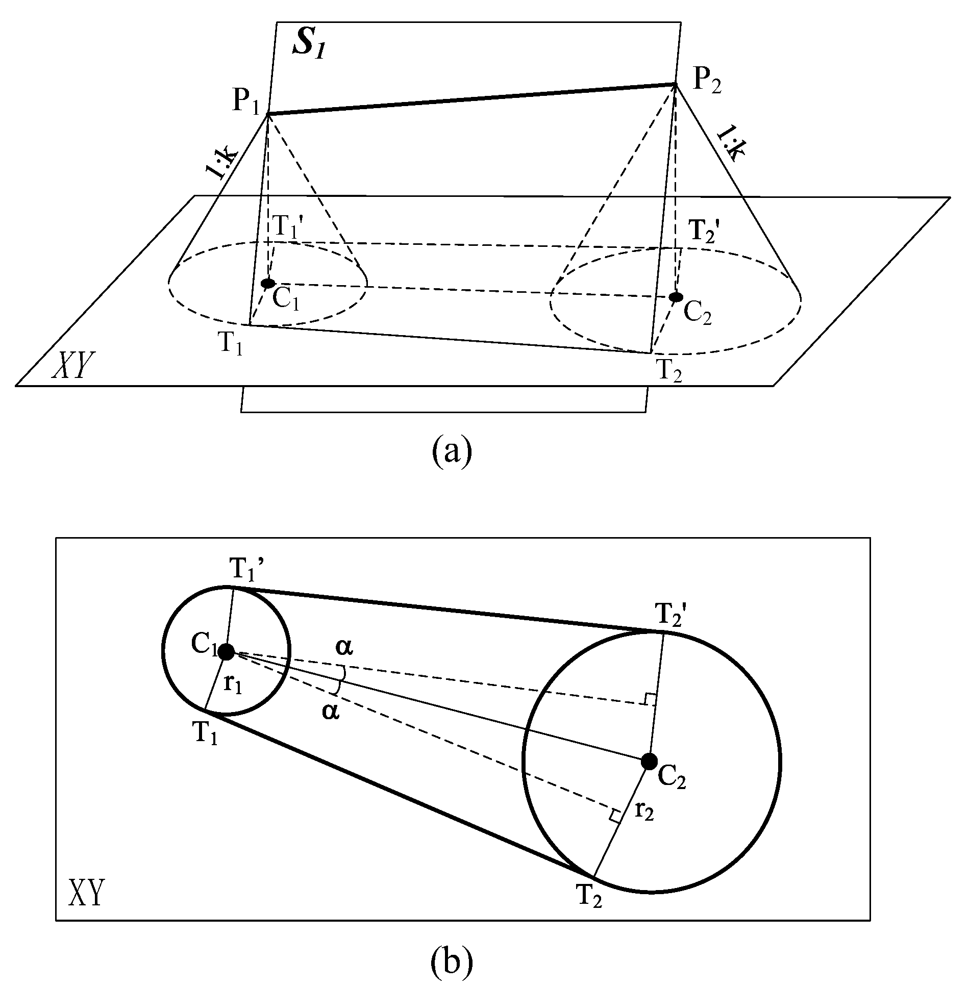
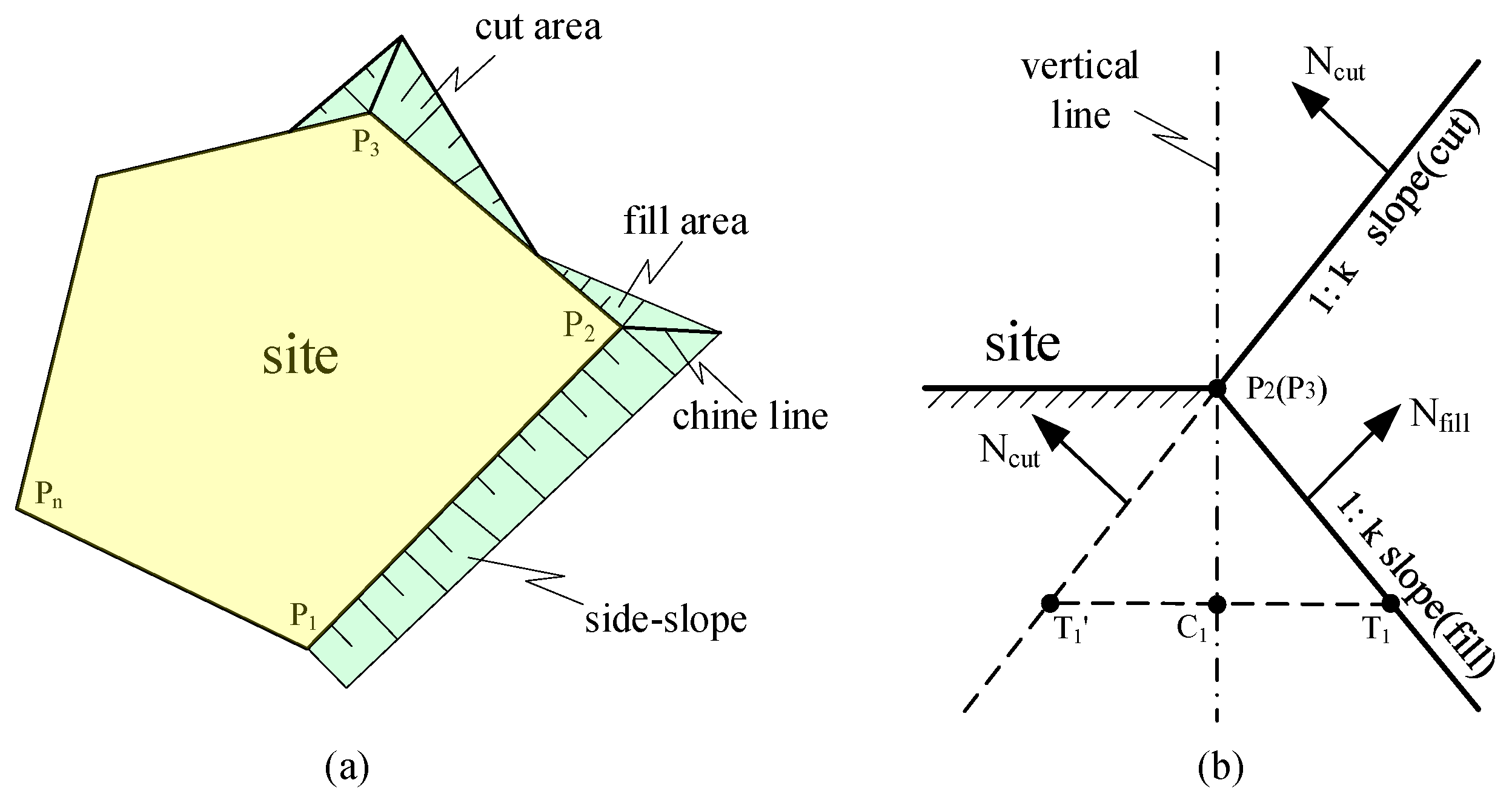
2.1. Side-Slope Plane Equation

The boundary lines P₁, P₂, …P_n of a known site is a spatial polyline. Consider its first segment P₁P₂; the side-slope plane S₁ passes through this line segment, and the side-slope of the plane is 1: k, see Figure 1a. Construct two right cones, their vertices are P₁ and P₂ respectively, and the cone slope is 1: k. Obviously, plane S₁ is tangent to these two cones, and the intersection points of its tangent line and the XY plane are T₁ and T₂, respectively. To find the plane S₁, let us calculate the point T₁. As shown in Figure 1b, the circle centers C₁ and C₂ are, respectively, the projection points of P₁ = (x₁, y₁, z₁) and P₂ = (x₂, y₂, z₂) on the XY plane. Since the slope of the cone is 1: k, the radii of the two circles r₁ = k·z₁ and r₂ = k·z₂ are obtained.

Let a = x₂ − x₁, b = y₂ − y₁, and c = z₂ − z₁; the angle α is given by

$$\alpha =\arcsin {\displaystyle \frac{r_2-r_1}{\left|C_1{C}_2\right|}}=\arcsin {\displaystyle \frac{kc}{\sqrt{a^2+b^2}}}$$

(1)

Next, the geometric transformation method is used to find T₁ as follows: C₂ rotates 90° + α clockwise around C₁, and then scales r₁/|C₁C₂| proportionally, and T₁ is obtained. For these, we apply four transformations to C₂ as

T₁ = M4·M3·M2·M1·C₂

(2)

Among them, M1, M2, M3, and M4 are four matrices, which are responsible for translation, rotation, scaling, and translation back, respectively:

$$M1=\left[\begin{array}{ccc}1& 0& {-\mathrm{x}}_1\\ 0& 1& {-\mathrm{y}}_1\\ 0& 0& 1\end{array}\right],$$

(3)

$$M2=\left[\begin{array}{ccc}\cos ({\displaystyle \frac{\pi }{2}}+\alpha )& \sin ({\displaystyle \frac{\pi }{2}}+\alpha )& 0\\ -\sin ({\displaystyle \frac{\pi }{2}}+\alpha )& \cos ({\displaystyle \frac{\pi }{2}}+\alpha )& 0\\ 0& 0& 1\end{array}\right],$$

(4)

$$M3=\left[\begin{array}{ccc}{\displaystyle \frac{k{z}_1}{\sqrt{a^2+b^2}}}& 0& 0\\ 0& {\displaystyle \frac{k{z}_1}{\sqrt{a^2+b^2}}}& 0\\ 0& 0& 1\end{array}\right],$$

(5)

$$M4=\left[\begin{array}{ccc}1& 0& {\mathrm{x}}_1\\ 0& 1& {\mathrm{y}}_1\\ 0& 0& 1\end{array}\right]$$

(6)

From (1) and (2), the vector P₁T₁ is calculated by

$$P_1{T}_1=z_1\left[k{\displaystyle \frac{-kac+b\sqrt{a^2+b^2-k^2{c}^2}}{a^2+b^2}},k{\displaystyle \frac{-kbc-a\sqrt{a^2+b^2-k^2{c}^2}}{a^2+b^2}},-1\right]$$

(7)

Use the same method to obtain P₁T₁′

$$P_1{T}_1^{\prime }=z_1\left[k{\displaystyle \frac{-kac-b\sqrt{a^2+b^2-k^2{c}^2}}{a^2+b^2}},k{\displaystyle \frac{-kbc+a\sqrt{a^2+b^2-k^2{c}^2}}{a^2+b^2}},-1\right]$$

(8)

Passing through the line segment P₂P₃, there are two planes with a slope of 1: k to the XY plane. These two planes, respectively, represent two types of side-slopes in earthworks, shown in Figure 2. One is an upward slope and the other is a downward slope. The height value of the point on the upward slope is greater than the site height, which is called the slope of cut type; conversely, the downward slope is smaller than the site height, which is the fill type. Because the site boundary lines P₁P₂…P_n are arranged counterclockwise, when moving along the boundary line, the site is always on the left and the slope is always on the right, see Figure 2. The fill side-slope is determined by three points, T₁, P₁, and P₂, while the cut side-slope is determined by three points, T₁′, P₁, and P₂. Thus, we can calculate the unit normal vectors N_fill and N_cut of the fill side-slope S₁ and the cut side-slope S₁′, respectively.

$$\begin{array}{l}{N}_{fill}={\displaystyle \frac{P_1{T}_1\times P_1{P}_2}{|P_1{T}_1\times P_1{P}_2|}}\\ =\left[{\displaystyle \frac{-kac+b\sqrt{a^2+b^2-k^2{c}^2}}{(a^2+b^2)\sqrt{1+k^2}}},{\displaystyle \frac{-kbc-a\sqrt{a^2+b^2-k^2{c}^2}}{(a^2+b^2)\sqrt{1+k^2}}},{\displaystyle \frac{k}{\sqrt{1+k^2}}}\right]\end{array}$$

(9)

$$\begin{array}{l}{N}_{cut}={\displaystyle \frac{P_1{P}_2\times P_1{T}_1^{\prime }}{|P_1{P}_2\times P_1{T}_1^{\prime }|}}\\ =\left[{\displaystyle \frac{-kac-b\sqrt{a^2+b^2-k^2{c}^2}}{(a^2+b^2)\sqrt{1+k^2}}},{\displaystyle \frac{-kbc+a\sqrt{a^2+b^2-k^2{c}^2}}{(a^2+b^2)\sqrt{1+k^2}}},{\displaystyle \frac{k}{\sqrt{1+k^2}}}\right]\end{array}$$

(10)

Add the fill/cut mark L = ±1, and unify the two formulas above as:

$$N=\left[\begin{array}{l}{\displaystyle \frac{-kac+L\cdot b\sqrt{a^2+b^2-k^2{c}^2}}{(a^2+b^2)\sqrt{1+k^2}}},\\ {\displaystyle \frac{-kbc-L\cdot a\sqrt{a^2+b^2-k^2{c}^2}}{(a^2+b^2)\sqrt{1+k^2}}},\\ {\displaystyle \frac{k}{\sqrt{1+k^2}}}\end{array}\right]$$

(11)

When L = 1, it signifies N_fill; when L = −1, it denotes N_cut. The value of L can be automatically determined using the method described in Section 3.

Thus, given two points P₁(x₁, y₁, z₁), P₂(x₂, y₂, z₂), and the slope value k, the normal vector N (N_x, N_y, N_z) of the side-slope plane is obtained. Then, we have the algebraic equation of the side-slope plane:

$$\begin{array}{l}{N}_x\mathrm{x}+N_y\mathrm{y}+N_z\mathrm{z}+D=0,\\ whereD=-(N_x{x}_1+N_y{y}_1+N_z{z}_1)\end{array}$$

(12)

At the turning points of the site boundary, two side-slope planes intersect to form a chine line. The line can be obtained by these two side-slope planes. Let N₁ and N₂ be the normal vectors of two planes. If the chine line shoots out through the turn point P, then the directional vector of the chine line is the cross product of the two normal vectors. The parametric equation of the chine line is as follows, with t as the parameter:

$$R(t)=P+(N_2\times N_1)\cdot t$$

(13)

2.2. Terrain Triangle Meshes

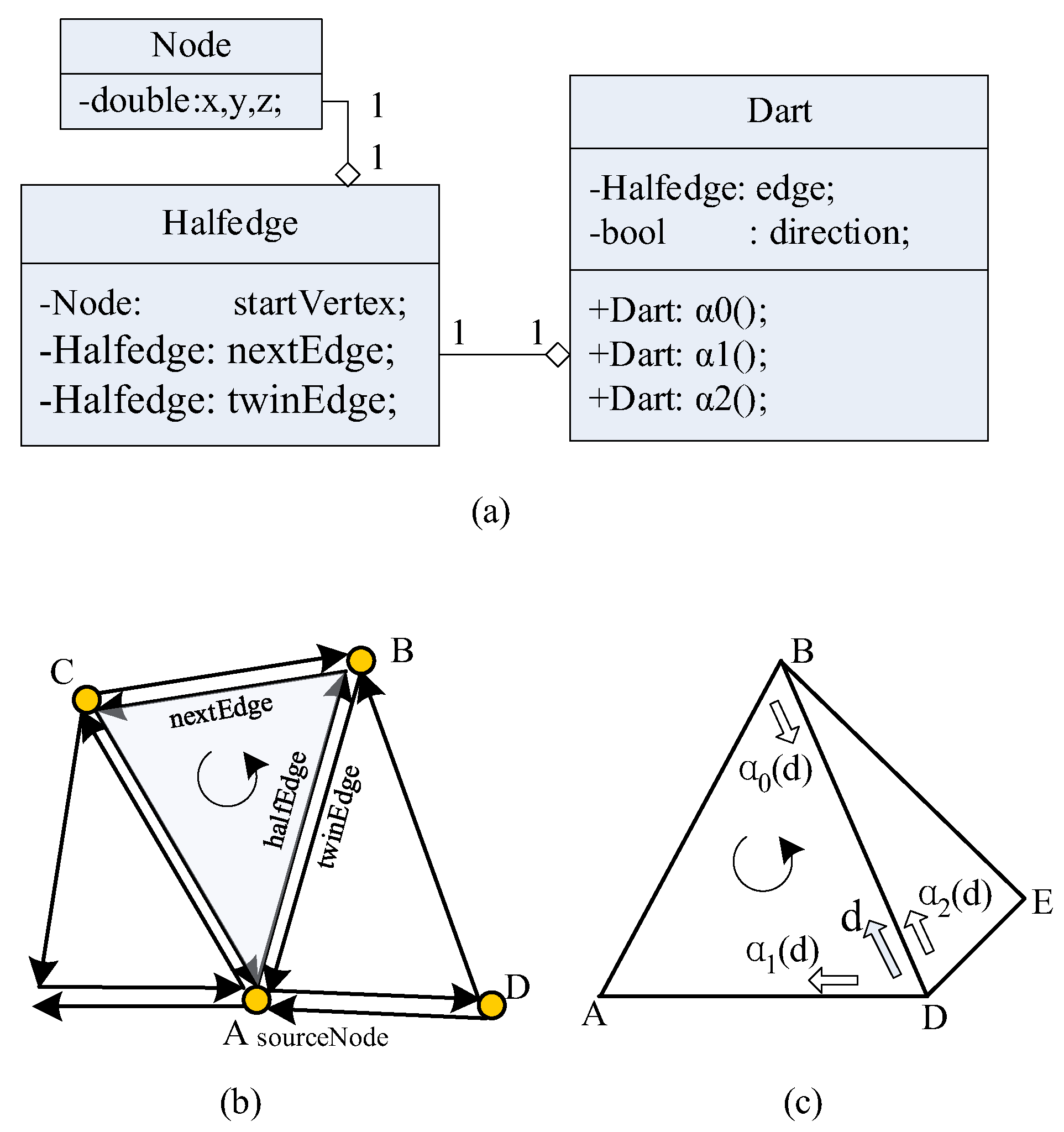
2.2.1. Half-Edge Data Structure

Commonly used data structures for representing triangle meshes include [17] the winged-edge, quad-edge, and half-edge structure. Among them, the half-edge structure splits an edge into two half-edges with opposite directions, which provides excellent topological querying capabilities. In this paper, this data structure is used to represent terrain surface.

As shown in Figure 3a, the half-edge data structure includes a start vertex and two half-edge pointers which point to the nextEdge and the twinEdge accordingly. The former points to the next counterclockwise adjacent edge within the same triangle, the latter points to the opposite edge in the adjacent triangle. A triangle is composed of three half-edges connected counterclockwise, as illustrated in Figure 3b. Each half-edge carries geometric and topological information; knowing one half-edge is sufficient to determine the triangle. Taking half-edge AB as an example in the triangle of ∆ABC (Figure 3b), we can access BC by AB → nextEdge, and CA by AB → nextEdge → nextEdge. Also, we can visit the adjacency triangle of ∆ADB by AB → twinEdge. Thereby the topological adjacency relationship in the whole of triangle mesh will be obtained.

In order to make the topological query more convenient, the Dart data structure is used. Dart adds a direction member within the half-edge to indicate whether the direction of edge is positive or negative.

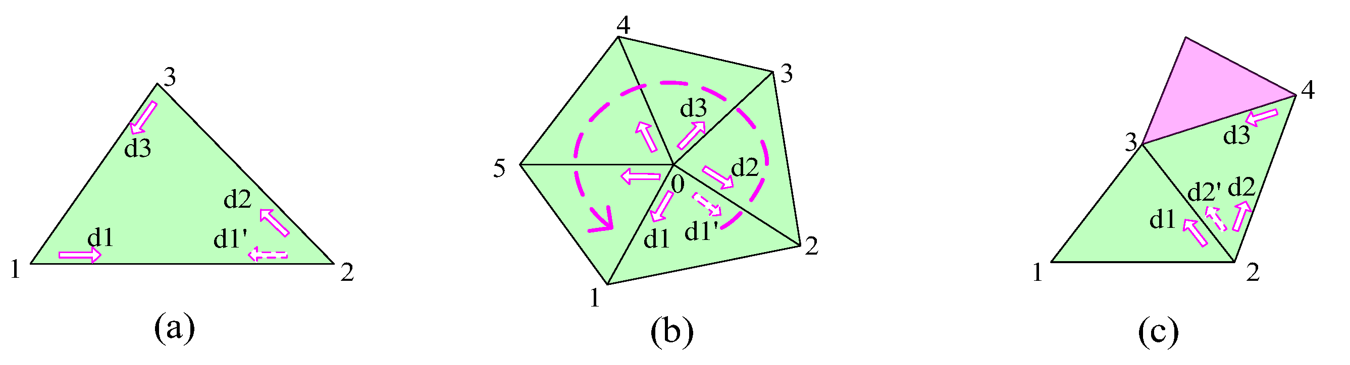
2.2.2. Topological Combination Operations

Dart can also be regarded as a triplet (v, e, t) composed of vertex, edge, and face [18]. Using the triplet, we define three basic topological operators: α₀(), α₁(), and α₂().

Let d = (D, DB, ∆ADB), shown in Figure 3c. We have:

α₀(d) = (B, DB, ∆ADB)

α1(d) = (D, DA, ∆ADB)

α2(d) = (D, DB, ∆BDE)

These three basic operations can be combined to perform more complex topological operations. The following introduces three α-combination operations that will be used in the intersection algorithm of this paper.

① Edges traversal inside a triangle

As shown in Figure 4a, given that d1 = (1, 12, ∆123), then d1′ = α₀(d1), d2 = α₁(d1′) = α₁ · α₀(d1), and d3 = α₁ · α₀(d2) = α₁ · α₀ · α₁ · α₀(d1). Here, by repeatedly using the α₁ · α₀ operation, one can traverse all the edges of a triangle in a counterclockwise direction.

② Umbrella traversal

Umbrella traversal refers to the sequential visiting all triangles that share a common point. In Figure 4b, there are five triangles shaped like an umbrella that share point 0 as their common point. Given that d1 = (0, 01, ∆012), then d1′ = α₁(d1), d2 = α₂(d1′)=α₂ · α₁(d1), d3 = α₂ · α₁(d2) = α₂ · α₁ · α₂ · α₁(d1), and so on. So, by repeatedly using the α₂ · α₁ operation, one can traverse all triangles sharing a common point in a counterclockwise direction.

③ Accessing the edges of adjacent triangle

In Figure 4c, given d1 in ∆123, entering adjacent triangle ∆324 by d2′ = α₂(d1). Next, d2 = α₁(d2′) = α₁ · α₂(d1), d3 = α₁ · α₀ · α₁ · α₂(d1).

3. The First Stage

As seen in Section 2.1, calculating the side-slope equation requires first determining its type. In this section, by analyzing the changes in fill and excavation types on side-slope surfaces, a rule for inferring changes in fill and excavation types based on intersection points is proposed. Then, a method to quickly calculate the intersection point between the boundary line and the terrain surface is given. Through the first stage process, all side-slopes can be established in sections along the boundary lines.

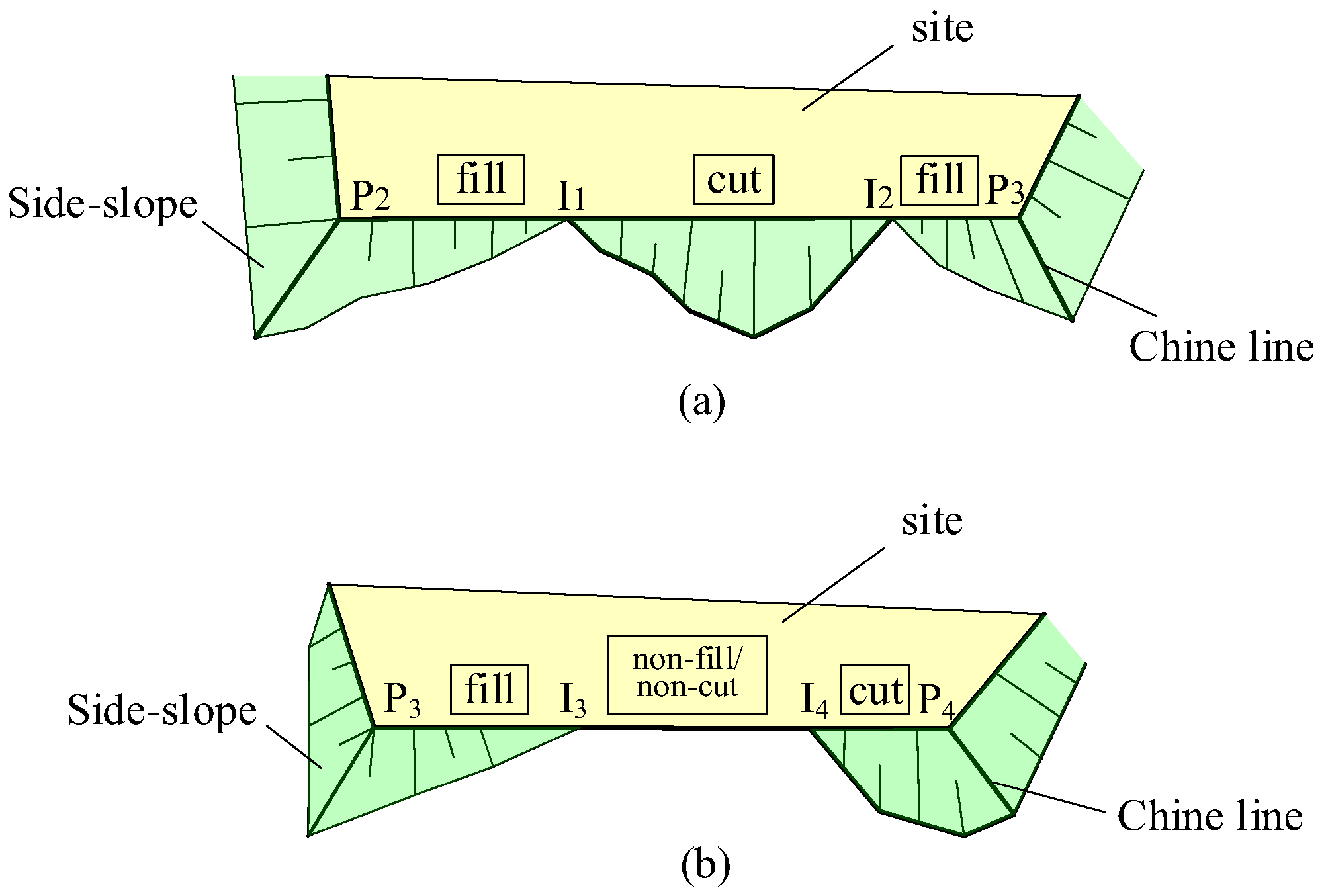
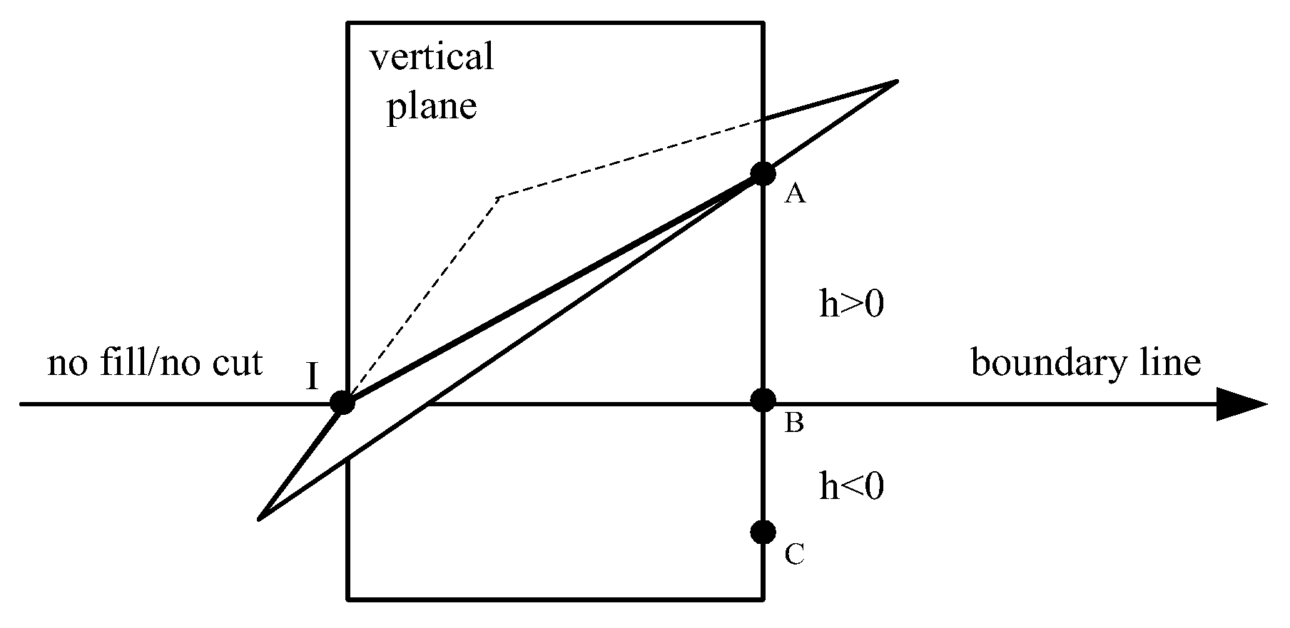
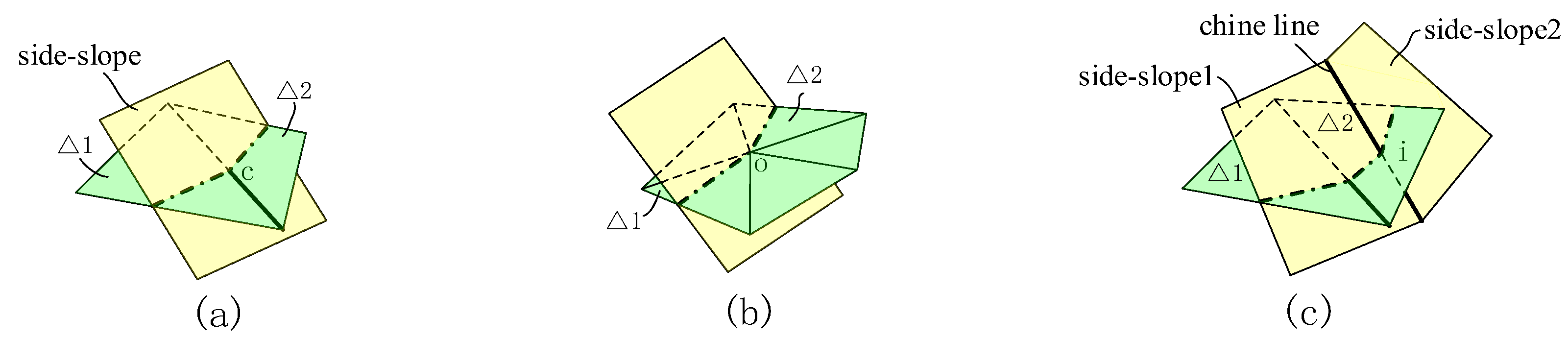
3.1. Rules for Changes in Fill/Cut Side-Slope Types

As traveling along the site boundary lines, the boundary will be divided into segments due to the undulations of the terrain. Some segments are above the ground (fill segments) and some are below (cut segments). One method to determine the type of cut and fill is to sample, which is to take a series of sampling points on the boundary line and compare the height difference between the sampling points and the terrain surface. However, this method is affected by the sampling density. To this end, a new method is proposed that divides fill and cut segments through intersection points and uses continuity to deduce fill or cut types.

By observation, the fill/cut type on the boundary line does not change until the intersection point with the terrain surface is encountered. Therefore, the intersection point is the key to triggering a change in fill/cut type. Calculate all intersection points between the boundary line and the terrain surface and then divide the boundary lines into fill/cut segments. Taking Figure 5a as an example, on the P₂P₃ boundary line, I₁ and I₂ are the intersection points. To the left of I₁, the side-slope type is fill. As it nears I₁, the side-slope length shortens until it diminishes to zero. After passing I₁, entering the next side-slope, the type of it changes to cut. For point I₂, the fill/cut type is similarly flipped once. To sum up, every time when passing through an intersection, the type of side-slope will be reversed, such as fill → cut → fill → cut →…and so on. Another situation needs to be considered here. For the intersection points I₃ and I₄ in Figure 5b, the I₃I₄ segment are coplanar with the terrain surface, so this section happens to be neither filled nor excavated.

Next, by analyzing the spatial relationship between the boundary line and the terrain triangle, we discuss how the cut and fill type changes. There are three situations of spatial relationships: intersecting, coplanar, and disjoint.

① When the boundary line intersects the triangle surface space, part of the triangle is higher than the boundary line and part is lower than the boundary line. The higher part is within the excavation range, and the lower part is within the fill range. Therefore, after such an intersection, the type of side-slope fill/cut will exchange.

② When the boundary line is coplanar with the triangular plane (meaning it has an intersection with both sides), there will be no height difference, no filling and no excavation (that is, non-fill/non-cut segment). So, this segment will not produce side-slope.

③ If the boundary line and the triangular surface do not intersect or are coplanar, it will not affect the fill and cut type of the side-slope.

Through the above analysis, all situations and changing conditions of excavation and filling changes are listed, see

Table 1. Rules of conversion on fill/cut type of side-slope.

No.	Spatial Relationship Between Boundary Line and Triangle Surface	Change in Fill/Cut Type
1	Intersecting and Intersection Point Inside the Triangle	Reversal at the intersection point, either from fill to excavation or from excavation to fill
2	Intersecting and Intersection Point on One Side of the Triangle	No change in fill/cut type
3	Coplanar (two intersection points on the triangle edge)	This segment becomes neither fill nor excavation; the type of the next segment is determined by the method in Figure 6
4	Not Intersecting	No change in fill/cut type

. In the third and second situations in the table, the excavation and fill types change irregularly and require further judgment. To this end, we can calculate the intersection line between the vertical plane where the boundary line is located and the triangular plane where the intersection point is located, as shown in Figure 6. Point B is the intersection point when the boundary line and the triangular plane are coplanar, and points A and C are above and below point B, respectively. Corresponding to these three situations, it is determined that the three types of the new interval are fill, non-fill/non-cut, or cut.

To summarize, the necessary condition for judging the change in side-slope fill/cut type along the boundary line is that the boundary line has an intersection with the terrain mesh, but the intersection does not necessarily lead to a change in the side-slope type. The judgment rules are as follows.

Rule 1.

When the intersection is an internal intersection (corresponding to the first case in Table 1), it inevitably leads to a change in side-slope type, at which intersection point the excavation and filling types reverse; if the last section is filling, this section must be excavation, and vice versa. When the intersection point is the intersection point on the edge of the triangle (corresponding to the 2nd and 3rd situations in Table 1), it does not necessarily lead to a change in the side-slope type. In this case, the first boundary line passing through the intersection point needs to be taken. A triangular surface is used to determine the side-slope excavation and fill type of the next boundary line. Finally, if there is no intersection (corresponding to the fourth situation in Table 1), the side-slope fill/cut type will not change.

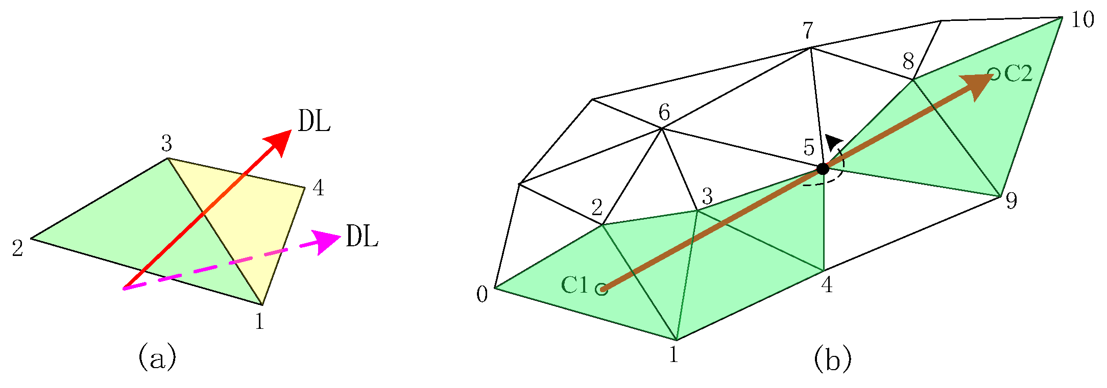
3.2. Finding the Intersecting Triangles in Mesh

From the above analysis, finding the intersection point between the boundary line and the terrain mesh is the key to determining the fill/cut type of side-slope. Using the half-edge structure, the number of intersecting triangle patches to be processed can be significantly reduced. The basic idea is as follows. First, in 2D space, we use the topological query of the half-edge structure to identify all triangles that intersect with the boundary line. Then, in three-dimensional space, we need to determine the exact intersection points between the boundary line and the space triangles.

Examine the topological relationship between the intersection of the directed line and the triangle on the plane, as shown in Figure 7a. If the directed line DL intersects edge 13 of ∆132, then the next intersecting triangle is the adjacent triangle ∆143, which shares the common edge 13. When entering in ∆143, the next intersecting edge can only be the edge 14 or the edge 43. In order to determine which edge it is, we just determine whether the vertex 4 is on the left of the directed line or not. If so, the next intersecting edge is edge 14, otherwise it is edge 43. Figure 7b is the complete process of traversing the triangular mesh to be intersected, where the triangles found are ∆012 → ∆132 → ∆143 → ∆453 → ∆598 → ∆9108.

While traversing along the specified path, it is crucial to swiftly identify the triangles within which points C1 and C2 are situated. Additionally, we must ascertain whether the vertices of these triangles lie to the left of the directed line. We adopt the locateTriangle algorithm and Left predicate by O’Rourke [19].

3.3. Calculation of Intersection Points Between Boundary Lines and Terrain Mesh

Once obtaining all intersecting triangles with the directed line in the two-dimensional space, we compute the spatial intersection point between the three-dimensional boundary line and the plane which is determined by each triangle. Let the equation of this plane be: n·P + D = 0. The two endpoints of the boundary line segment are P₁ and P₂, and its straight-line parameter equation is: P(t) = P₁ + t·(P₂ − P₁). If n·(P₂ − P₁) ≠ 0, the boundary line intersects the plane where the triangular surface is located. Bringing the boundary line parameter equation into the plane equation, we obtain t = (n·P₁ + D)/n·(P₁ − P₂). Therefore, the intersection point of the straight line and the plane is:

$$I=P_1+\frac{n·P_1+D}{n·(P_1-P_2)}\times (P_2-P_1)$$

(14)

Next, we use the locateTriangle algorithm to examine whether the point I is in the triangle. Only those points that satisfy the location conditions are the exact intersection points.

3.4. Determine the Side-Slope Type and Its Equation Piece by Piece

For the entire boundary line, the algorithm along the line calculates the intersection points, and then sorts the intersection points and boundary line turning points in counterclockwise order to form an ordered point set. Take two points from the point set to calculate the side-slope equation of each section. Specific steps see Algorithm 1.

Algorithm 1. Traveling-along-lines

Input: Terrain mesh M, boundary lines PL, slope value kfill and kcut.    Output: Side-slope equations for each segment on the boundary line, Eqs{}    ordered point set (turning point + intersection point).    1. Fetch the first turning points P1 of PL    2. ∆t: = locateTriangle (P1, M)    3. IF above (P1, ∆t) THEN L: = 1    4. ELSE L: = −1    5. IF (L == 1) THEN k: = kfill    6. ELSE k: = kcut    7. FOREACH (P1,P2) IN PL segments    8.   P: = P1    9.   Ints: = intersect (P1P2, M)    10.       FOREACH I IN Ints    11.      IF L == 0 THEN continue    12.      Eqs←side-slopeEq (P, I, L, k)    13.      L: = −1*L    14.      P: = I    15.  Eqs←side-slopeEq (P, P2, L, k)

4. The Second Stage

In this section, we use continuity to quickly calculate the intersection between each side-slope plane and the terrain mesh.

4.1. Topological Continuity of the Intersection Between the Side-Slope Plane and the Triangular Mesh

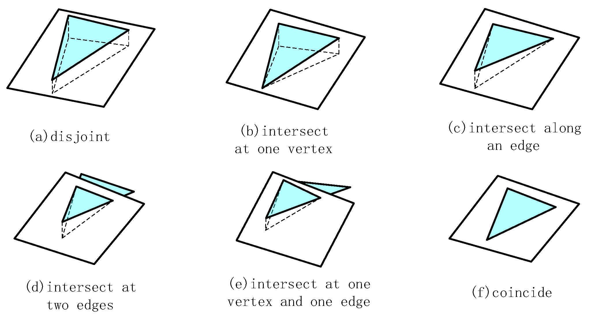
4.1.1. Spatial Relationship Between Plane and Triangle

There are three positional relationships between a point and a plane in space: above the plane, on the plane, and below the plane. Therefore, for three vertices of a triangle, there will be 3³ = 27 possible combinations of positional relationships. Considering symmetry, the 27 relationships can be combined into the following 6 types: ① three vertices are on one side of the plane (do not intersect); ② one vertex is on the plane and the other two vertices are on one side of the plane (intersect at one point); ③ two vertices are on the plane (intersects on one side); ④ one vertex is on one side of the plane and the other two vertices are on the other side of the plane (intersects on both sides); ⑤ one vertex is on the plane and the other two vertices are on different sides of the plane (intersects on one point and one side); and ⑥ the three vertices are all on the plane (coincident), see Figure 8.

4.1.2. Topological Continuity Analysis

The triangular mesh is composed of continuous triangles, so the intersection between the side-slope and the triangular mesh is also continuous. According to the spatial relationship between a plane and a triangle, if a plane intersects the first side of a triangle, then the next intersection can only be the vertex or another side of the triangle. In this way, the intersection between the side-slope surface and the triangular mesh has three continuous situations. ① Figure 9a: when the side-slope surface intersects ∆1, it also intersects ∆2 which is adjacent to ∆1. The side-slope connects with the intersection segments of the two triangles at point c on the common edge. ② Figure 9b: if the side-slope intersects at the vertex o of ∆1, then the next triangle that intersects the side-slope is a triangle with o as the common point. The side-slope connects with the intersection segment of the two triangles at the common point o. ③ Figure 9c: two intersecting side-slopes intersect with the same ∆2, then ∆2 has two intersection segments with each of the two side-slopes, and the two segments meet at the intersection i of the chine line and ∆2.

4.2. Algorithm of Traveling Along Plane

Determining which side of the plane a point is on is called lateral judgment of the point plane. It is known that the plane equation is Ax + By + Cz + D = 0; let the function e(x,y,z) = Ax + By + Cz + D. For any point P(x,y,z), if e(P) > 0, then P is on one side of the normal vector direction of the plane; if e(P) < 0, on the other side, such as e(P) = 0, then P is on the plane. Obviously, for a line segment, if its two endpoints are on different sides of the plane, the line segment intersects the plane.

Similarly to the traveling-along-line algorithm (Algorithm 1), the traveling along plane algorithm also uses the properties of the half-edge structure to quickly traverse the triangles to be intersected. The main difference is that the intersection line is not on a straight line but on a plane, and the point-surface lateral judgment is used to determine whether the edge intersects the surface.

4.3. Calculation of the Intersection Line Between the Side-Slope Surface and the Terrain Mesh

The method of finding the intersection between a side-slope group and a triangular mesh is to find the intersection lines with the triangular mesh for each side-slope in the group one by one. During the intersection process, the first triangle that intersects with the side-slope group is found, and then the triangles to be intersected are found one by one using the surface traveling algorithm. When the intersection line encounters a chine line, it goes to the next side-slope, and the side-slope group is processed in this loop until the last side-slope. Specific steps see Algorithm 2.

Algorithm 2. Traveling-along-planes

Input: Boundary lines PL, equations of side-slope planes {Eqs}, terrain mesh M.    Output: The intersection lines {INTs} between side-slope planes and terrain mesh.    1. Find the first triangle that intersects the side-slope    2. R(t) = P1 + (N2 × N1) · t   //See Equation (13)    3. i: = intersect (R(t), M)    4. ∆t: = locateTriangle (i,M)    5. FOREACH side-slope plane sp IN Eqs:    6.    ∆t2: = locateTriangle (P2, M)    7.    WHILE ∆t ≠ ∆t2 DO:    8.     INTs←INTs +intersect (sp, ∆t)    9.     ∆t: = AdjcentTriangle (sp, ∆t)

5. Discussion

On the Visual Studio 2019 platform, the C++ development language and the OpenGL graphics library and the open source library TTL (Triangulation Template Library) provided by Hjelle [20] were used to implement the algorithm proposed above. Hardware environment: CPU: Intel i5, memory: 4.0GB (Intel Corporation, Santa Clara, CA, USA).

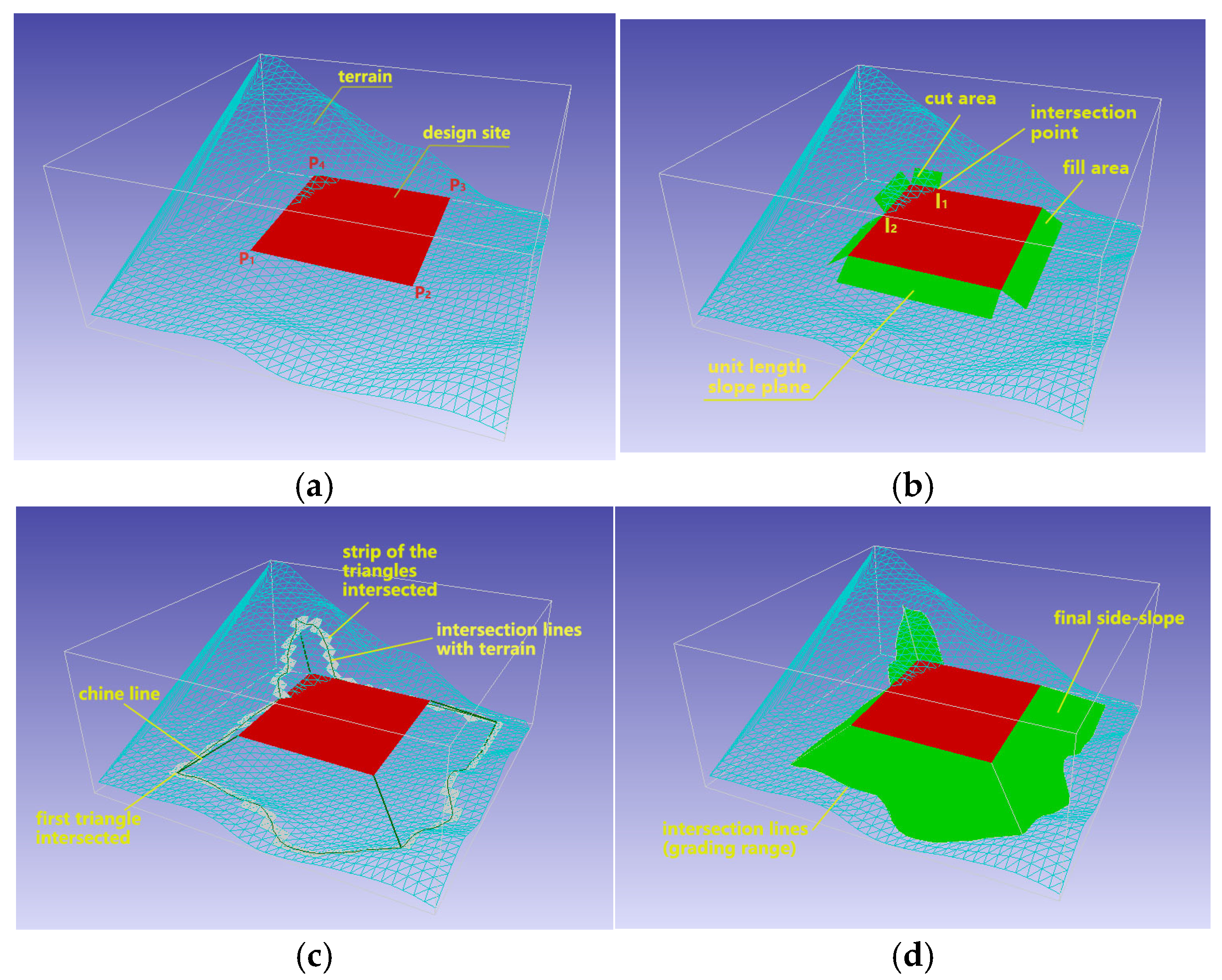
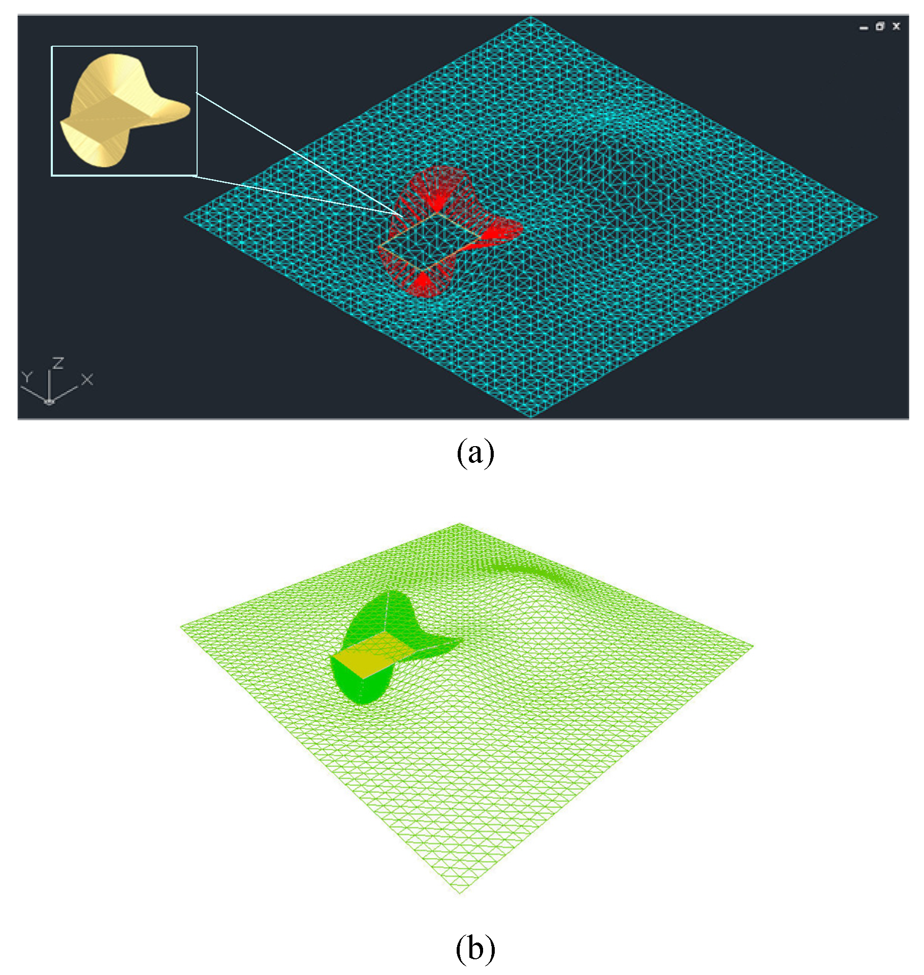
5.1. Examples

The original terrain data are derived from survey points of an actual engineering project. Using the TTL and the point data, a terrain mesh was generated. As shown in Figure 10a, there are a total of 1482 vertices and 2848 triangles in the original terrain triangulation mesh. The design site is a rectangular area with four turning points: P₁ (8709.00, 7992.00, 15.00), P₂ (8712.00, 8050.00, 15.00), P₃ (8695.00, 8045.00, 15.00), and P₄ (8690.00, 7980.00, 15.00)—and the cut and fill grade adopted are 1:0.75 and 1:1.5, respectively. The site turning point P₄ is lower than the terrain surface, and the other three turning points are higher than the terrain, so it is a half-filled and half-excavated site.

Figure 10b shows the first stage of the proposed method. Using Algorithm 1, traveling along the boundary polyline P₁P₂P₃P₄, two spatial intersection points I₁ and I₂ between the boundary line and the terrain mesh are calculated, so that the entire boundary line is divided into six segments. First, we determine that the point P₁ is above the terrain mesh, so it is in the fill section. Then, we deduce the fill/cut type of subsequent sections by the Rule 1.

Table 2. Segmented calculation of side-slope plane.

No.	Start Point	Point Type	End Point	Inverse	Fill/Cut Type	L Sign	Slope Value
1	P1	Turning Point	P2	false	fill	1	1:1.5
2	P2	Turning Point	P3	false	fill	1	1:1.5
3	P3	Turning Point	I1	false	fill	1	1:1.5
4	I1	Intersection Point	P4	true	cut	−1	1:0.75
5	P4	Turning Point	I2	false	cut	−1	1:0.75
6	I2	Intersection Point	P1	true	fill	1	1:0.75

provides a detailed process for deducing the fill/cut type of six sections. Finally, the fill/cut type for each side-slope is identified, totaling four filling and two excavating ones.

Using the results from Table 2, we can then establish the equation of each side-slope plane. Taking the first row of Table 2 as an example, we show how to compute it. From the first row, we obtain parameters of the first side-slope plane, as follows:

a = P₂[0] − P₁[0]

b = P₂[1] − P₁[1]

c = P₂[2] − P₁[2]

L = 1, k = 1:1.5

Then, substituting the above parameters into Equation (11), we obtain the normal of the first side-slope plane:

N_P2P1 = [−0.55, 0.03, 0.83],

and the plane equation:

−0.55x + 0.03y + 0.83z + 4582.96 = 0

In the same way, we can obtain all side-slope planes, which are temporarily drawn according to the unit slope length in Figure 10b.

The second stage of the method proposed is shown in Figure 10c, in the process of calculating the intersection along the side-slope plane using Algorithm 2. First, we should find the first triangle intersected by computing the first chine line hitting the mesh. Using Equation (13), we have the equation of the chine line:

R(t) = P₁ + (N_P2P1 × N _P1I2)·t = [8709.00, 7992.00, 15.00] + [−0.37, 0.21, −0.25]·t

After identifying the first intersecting triangle, the marching algorithm is then used to determine all intersecting triangles sequentially. In Figure 10c, the gray triangles in the mesh are those that have been identified as intersected. Figure 10c also shows four chine lines at the corners and the final intersection lines between the side-slope plane and the triangular mesh. Figure 10d shows the final result after rendering the side-slope surfaces.

The traversal process in the proposed method relies on the continuity of triangles within the terrain mesh. Therefore, when there are holes in the mesh, the continuity of the traversal will be affected. This method is not only applicable to site modeling but can also be used for embankments, riverbanks, and similar structures. Figure 11 is an example of modeling a terrace site and a road embankment using the method proposed in the paper. The boundary lines of the embankment in the figure should be curved at the turning point. In order to use the method proposed, multi-segment polylines are applied to approximate the curve and generate the subgrade side-slope model.

The Algorithm 2 in this article can also be used to calculate stratigraphic profiles. At this time, the side-slope surface becomes a section plane, and each layer is still a triangular mesh surface. The stratigraphic profiles are obtained by calculating the intersection lines between the section plane and the stratigraphic triangular mesh, see Figure 12.

5.2. Analysis

The main access operations of our two-stage method proposed in this article are point positioning and lines/planes traversal. The average time complexity of the algorithm for point positioning operations is O (logN) (N is the number of triangles in the mesh). For the marching algorithm along lines/planes, only a narrow strip of the terrain mesh is traversed, rather than the entire set of triangles within the mesh. Additionally, the topological combination operations based on the half-edge structure mentioned above also significantly enhance the traversal speed during the marching process. In order to estimate the relationship between algorithm efficiency and the number of triangles in the mesh, the terrain triangular mesh depicted in Figure 10 is subdivided.

Table 3. Variation of calculation time with the number of triangles.

Total Number of Triangles in the Mesh	Number of Intersecting Triangles	Time (ms)
2848	254	2.5682
8544	442	2.6644
14,240	551	2.9308
19,936	671	3.5895
25,632	750	4.1023
42,720	991	5.4027
59,808	1126	6.0809
71,200	1265	6.7120
76,892	1288	7.2347
99,680	1447	7.9305
128,160	1670	8.8576
139,552	1735	9.1974
213,600	2207	11.7620

shows the changes in the number of intersecting triangles during traversal and the total calculation time as the total number of triangles in the mesh increases. It can be observed from Figure 13 that the total number of triangles in the mesh and the number of intersecting triangles exhibit a non-linear relationship with a roughly parabolic trend, while the number of intersecting triangles and the calculation time show a roughly linear relationship. This linearity implies that the increase in calculation time is proportional to the increase in the number of intersecting triangles, which is a desirable property for algorithm scalability. However, the number of intersecting triangles is not linearly related to the total number of triangles, so the calculation time is non-linear with respect to the total number of triangles. The data in Table 3 further supports these observations. As the total number of triangles in the mesh increases, both the number of intersecting triangles and the calculation time also increase. However, the rate of increase in calculation time is not as steep as one might expect from a purely linear model, suggesting that the algorithm’s efficiency is relatively robust against increases in mesh complexity.

5.3. Comparison

The commercial software Civil3D 2016 [21] was used as a comparison with the method proposed in this section. The model is shown in Figure 14. In the figure, (a) is the three-dimensional wireframe diagram of the site and side-slope generated with Civil3D (the upper left corner is the rendering) and (b) is the three-dimensional diagram generated by the method in this section. Comparing the two figures, we can see that there is basically no difference between the two models in terms of fill and excavation segments, side-slope shape, etc. After testing, the total time for generating the side-slope model by the method proposed is 2.2 ms, while the time used by Civil3D is >200 ms, so the time efficiency improvement of this method is considerable. In addition, the algorithm in this paper is also compared with the intersection algorithm based on subdivision [22]. The comparison of algorithm time is shown in

Table 4. Calculating time comparison with intersection algorithm based on subdivision.

Total Number of Triangles in the Mesh	ZHAO [22] (ms)	The Method Proposed (ms)
~19,000	229	3.59
~139,000	2604	9.20
~250,000	5104	13.21

.

6. Conclusions

The two-stage method proposed in this paper is based on a traversal algorithm applied to the triangle mesh. By leveraging the continuity of the intersection lines and utilizing operations on the half-edge structure, the number of intersection triangles that need to be calculated is significantly reduced. This results in a method that is both fast and computationally efficient. The accuracy of the generated intersection lines is directly influenced by the precision of the terrain triangulation mesh. The proposed method reduces computational time while maintaining the necessary level of precision required for analyzing the interaction between the side-slope and the terrain. During the traversal process, the intersection points are automatically arranged in order, eliminating the need for additional sorting operations. The greatest convenience of this method is that, given the original terrain and site boundaries, it can automatically identify all side-slopes, determine their types, and calculate the intersections without requiring the interactive sample-line operations typically needed in software like Civil3D. This convenience makes the method particularly suitable for the preliminary planning stages of engineering projects such as site development and road construction. Designers simply need to sketch the boundaries of the site, and the method can rapidly calculate the earthwork area. With the generated 3D model, designers can adjust the plan and optimize the alignment more effectively. Of course, rapid model optimization will also benefit stakeholders.

The proposed method is founded on the side-slope boundary with polylines. However, this approach falls short when it comes to precisely depicting side-slopes with curved boundaries, due to the necessity for a novel surface equation. For surfaces with curved side-slopes, the fundamental concept of the two-stage algorithm introduced here remains viable. Nevertheless, adjustments are required for the point-line lateral direction determination algorithm employed in the traveling-along-lines algorithm; the cross-multiplication method is inadequate for ascertaining the lateral direction of points relative to curves, necessitating the development of an alternative approach. Additionally, in the traveling-along-planes algorithm, while the curve side-slope can be articulated as algebraic equations and point-surface lateral judgment algorithms remain effective, a new technique is essential for calculating the intersection between a triangle edge and a surface. Moreover, another important direction for future work is the integration of geological information into side-slope modeling. This includes the automatic matching of soil layer types and side-slope gradients, which can further enhance the algorithm’s level of automation. These improvements are planned for future research.

References

- Glaeser, G. Geometry and Its Applications in Arts, Nature and Technology; Springer International Publishing: Berlin/Heidelberg, Germany, 2020; pp. 201–206. [Google Scholar]
- Hare, W.; Lucet, Y.; Rahman, F. A mixed-integer linear programming model to optimize the vertical alignment considering blocks and side-slopes in road construction. Eur. J. Oper. Res. 2015, 241, 631–641. [Google Scholar] [CrossRef]
- Momo, N.S.; Hare, W.; Lucet, Y. Modeling side slopes in vertical alignment resource road construction using convex optimization. Comput. Aided Civ. Infrastruct. Eng. 2023, 38, 211–224. [Google Scholar] [CrossRef]
- Yuan, L.; Liu, S.; Meng, L. Numerical simulation analysis of slope stability from rainwater utilizing the Civil3D+Flac3D coupling. Desalin. Water Treat. 2024, 319, 100517–100527. [Google Scholar] [CrossRef]
- OpenRoads Designer, Roadway Design Software. Available online: https://www.bentley.com/software/openroads-designer/ (accessed on 12 September 2024).
- HintCAD. Available online: https://www.hintcad.cn/product/3862.html (accessed on 15 October 2024). (In Chinese).
- Hartmann, E. Geometry and Algorithms for Computer Aided Design; Darmstadt University of Technology: Darmstadt, Germany, 2003; Volume 95. [Google Scholar]
- Koźniewski, E.; Koźniewski, M.; Orłowski, M.; Owerczuk, J. Modeling an embankment with a natural slope. J. Biul. Pol. Soc. Geom. Eng. Graph. 2013, 25, 49–56. [Google Scholar]
- Zhou, F.; Li, C.; Ding, Y. Developable iso⁃slope surface and its application to slope modeling. J. Wuhan Univ. 2019, 52, 610–615. [Google Scholar]
- Yang, P.; Qian, X. Direct boolean intersection between acquired and designed geometry. Comput. Aided Des. 2009, 41, 81–94. [Google Scholar] [CrossRef]
- Lin, H.; Qin, Y.; Liao, H.; Xiong, Y. Affine arithmetic based B-Spline surface intersection with GPU acceleration. IEEE Trans. Vis. Comput. Graph. 2013, 20, 172–181. [Google Scholar]
- Shou, H.H.; Zhou, C. Triangular grid intersection based on hierarchical enclosing box and average cell. J. Zhejiang Univ. Technol. 2018, 46, 540–543+557. [Google Scholar]
- Shi, Y.F.; Zhang, Y.H.; Cheng, T. Intersection algorithm for surface segmentation based on space polygon triangulation. J. Graph. 2019, 40, 447–451. [Google Scholar]
- Elsheikh, M. A reliable triangular mesh intersection algorithm and its application in geological modelling. Eng. Comput. 2014, 30, 143–157. [Google Scholar] [CrossRef]
- Svelander, F.; Kettil, G.; Johnson, T.; Mark, A.; Logg, A.; Edelvik, F. Robust intersection of structured hexahedral meshes and degenerate triangle meshes with volume fraction applications. Numer. Algorithms 2018, 77, 1029–1068. [Google Scholar] [CrossRef]
- Ventura, M.; Guedes Soares, C. Surface intersection in geometric modeling of ship hulls. J. Mar. Sci. Technol. 2012, 17, 114–124. [Google Scholar] [CrossRef]
- Botsch, M.; Pauly, M.; Kobbelt, L.; Alliez, P.; Lévy, B.; Bischoff, S.; Röossl, C. Geometric Modeling Based on Polygonal Meshes. In Eurographics 2008 Tutorial Notes; Eurographics: Crete, Greece, 2008; pp. 17–18. [Google Scholar]
- Bradley, P.; Paul, N. Comparing G-maps with other topological data structures. GeoInformatica 2014, 18, 595–620. [Google Scholar] [CrossRef]
- O’Rourke, J. Computational Geometry in C; China Machine Press: Beijing, China, 2005; pp. 239–245. [Google Scholar]
- Hjelle, Ø.; Dæhlen, M. Triangulations and Applications; Springer Science & Business Media: Berlin/Heidelberg, Germany, 2006; pp. 25–28. [Google Scholar]
- Autodesk. AutoCAD Civil 3D. Available online: https://www.autodesk.com/products/civil-3d/ (accessed on 12 September 2024).
- Zhao, J.C.; Bai, R.C.; Liu, G.W. Research on TIN fast intersection algorithm and its application. Comput. Appl. Res. 2016, 33, 3667–3670+3695. [Google Scholar]