Existence and Uniqueness Results for Fuzzy Bipolar Metric Spaces

Abstract

In this paper, we present the concept of $(\mathrm{{\rm Y}},\mathrm{\Omega })$-iterativemappings in the setting of fuzzy bipolar metric space. The symmetric property in fuzzy bipolar metric spaces guarantees that the distance between any two elements remains invariant under permutation, ensuring consistency and uniformity in measurement regardless of the order in which the elements are considered. Furthermore, we prove several best proximity point results by utilizing $(\mathrm{{\rm Y}},\mathrm{\Omega })$-fuzzy bipolar proximal contraction, $(\mathrm{{\rm Y}},\mathrm{\Omega })$-Reich–Rus–Ciric type proximal contraction, $(\mathrm{{\rm Y}},\mathrm{\Omega })$-Kannan type proximal contraction and $(\mathrm{{\rm Y}},\mathrm{\Omega })$-Hardy–Rogers type contraction. Furthermore, we provide some non-trivial examples to show the comparison with the existing results in the literature. At the end, we present an application to find the existence and uniqueness of a solution of an integral equation by applying the main result.

1. Introduction

In 1922, Banach [1] gave an important result named the Banach contraction principle in fixed point theory (in short, FPT). Applications of FPT are found in many other fields of mathematics, including nonlinear analysis. It is an attractive and quickly expanding subject of study. Given that a map that adheres to the Banach contraction principle is continuous, it makes sense to inquire as to whether or not a discontinuous map fulfilling comparable contractive requirements has a fixed point. For this question Kannan [2] defined a contractive condition for discontinuous map R, as follows:

$$\mathrm{\Lambda }\left(R{s}^o,R{x}^o\right)\le h\left[\mathrm{\Lambda }\left(s^o,R{s}^o\right)+\mathrm{\Lambda }\left(x^o,R{x}^o\right)\right]$$

for all $s^o,x^o\in C$ and $h\in [0,\frac{1}{2})$. Moreover, he demonstrated the existence and uniqueness of FP in the setting of complete metric spaces.

The fuzzy set has gained popularity since Zadeh [3] introduced the fuzzy set theory in 1965 as a logical development of the idea of a set and laid the foundation for fuzzy mathematics. Schweizer and Sklar [4] presented the concept of continuous t-norm (CTN). In [5], a new concept of fuzzy space was introduced by combining the probabilistic metric spaces with the fuzzy set. This concept has applications in various mathematical disciplines, including logic, analysis and algebra, artificial intelligence, fixed point theory, and applied science fields like signal processing and medical imaging. Fuzzy sets have been widely used by numerous writers in a variety of mathematical fields. One of the most researched areas in fuzzy set theory is fuzzy metric spaces, which were first presented by Karamosil and Michalek [6]. Following that, a number of writers expanded and developed the idea of fuzzy metric space in different ways. By modifying the concept of fuzzy metric space, George and Veeramani [7], for instance, demonstrated that each fuzzy metric generates a Hausdorff topology.

First of all, Proinov [8] defined auxiliary function $\mathrm{{\rm Y}},\mathrm{\Omega }:\left(0,\infty \right)\to \mathbb{R}$ such that

(i)

$\mathrm{\Omega }\left(s^o\right)<\mathrm{{\rm Y}}\left(s^o\right)$ for any $s^o>0;$

(ii)

${inf}_{s^o>\epsilon }\mathrm{{\rm Y}}\left(s^o\right)>-\infty$ for any $\epsilon >0;$

(iii)

$\mathrm{{\rm Y}}$ is non-decreasing and $lim{sup}_{s^o\to \epsilon }\mathrm{{\rm Y}}\left(s^o\right)<\mathrm{{\rm Y}}\left(\epsilon +\right)$ for any $\epsilon >0;$

(iv)

If $\mathrm{{\rm Y}}\left({s^o}_n\right)$ and $\mathrm{\Omega }\left({s^o}_n\right)$ are convergent sequences with the same limit, $\mathrm{{\rm Y}}\left({s^o}_n\right)$ is strictly decreasing.

Moreover, he proved FPT and showed the existence of uniqueness of a fixed point for complete metric spaces. Hierro et al. [9] proved some auxiliary function in fuzzy metric space (in short, FMS) and showed FPT. Then, Zhou et al. [10] also improved the results of Hierro et al. [9]. Ishtiaq et al. [11] used auxiliary function and iterative mappings to find out FPT.

For non-self mapping, Basha [12] gave a new way to attain an optimal solution, which is the best proximity point (in short, BPP). Then, Jleli and Samet [13] found some BPP for $\left(\alpha ,\mathrm{\Psi }\right)$ proximal contractive mappings. Vetro and Salimi [14] showed BPP results in non-Archimedean FMS. Furthermore, Paknazar [15] found BPP results in non-Archimedean FMS. First of all, Farheen et al. [16] defined fuzzy multiplicative metric spaces and proved BPP for fuzzy multiplicative metric spaces. Some common BPP theorems were discussed in [17,18] by Ishtiaq et al. in FMS. Jahangeer et al. [19] found some BPP theorems by using iterative mappings in bipolar metric spaces. Alamri [20] developed fixed point theorems for F-bipolar metric spaces, expanding the concept of rational $(\wedge ,\vee ,\psi )$-contractions. These new contractions make it easier to derive fixed-point theorems for contravariant mappings. Maheswari et al. [21] extended fixed point theory by providing new theorems for bipolar fuzzy b-metric spaces. Their research gave a better understanding of fixed point existence and uniqueness in these generalized metric spaces. These new contractions not only increase the scope of fixed point theorems but they also generalize some well-known existence proofs from the literature.

The symmetric property plays a crucial role in establishing fixed points for contraction mappings by ensuring that the distance between any two elements remains invariant under permutation, which facilitates the analysis of convergence behavior. In the context of contraction mappings, symmetry ensures that the iterative application of the mapping yields consistent distances, preventing directional bias and enabling balanced error estimates. This property helps in proving the uniqueness of fixed points by allowing contraction conditions to hold uniformly in both forward and reverse directions, thus strengthening the validity of the Banach contraction principle and its extensions in fuzzy and bipolar metric spaces. Alnabulsi et al. [22] introduced several novel concepts within the framework of fuzzy bipolar b-metric spaces. They focused on various mappings, such as $\psi \alpha$-contractive and $\mathrm{{\rm Y}}\eta$-contractive mappings, which are essential to quantify distances between dissimilar elements. They developed fixed-point theorems for these mappings, establishing the existence of invariant points under specific conditions. Kumar et al. [23] proposed a generalized parametric bipolar metric space, which combines and expands the concepts of generalized parametric and bipolar metric spaces. They also presented Boyd–Wong type contractions for both covariant and contravariant mappings, which provided a framework for determining fixed point results in this newly defined space. Mani et al. [24] introduced Menger probabilistic bipolar metric spaces, along with related notions and definitions. They developed various novel fixed point theorems that handled both covariant and contravariant mappings. These theorems are novel generalizations of standard results such as the Banach contraction principle, Kannan theorem, and Reich-type theorem, tailored to the framework of Menger probabilistic bipolar metric spaces. Zararsiz and Riaz [25] defined fuzzy bipolar metric spaces (in short, FBMS) and their topological properties. In addition, Bartwal et al. [26] showed FPT in FBMS.

Routaray et al. [27] introduced the fuzzy differential transform method to solve a set of nonlinear fuzzy integro-differential equations. These equations are part of a mathematical model that depicts the coexistence of biological organisms. Acharya et al. [28] investigated the controllability of fuzzy solutions for second-order nonlocal impulsive neutral functional differential equations. Their study addresses both nonlocal and impulsive conditions in the fuzzy framework. Using the Banach fixed point theorem, they established a sufficient condition for controllability. Chalishajar and Ramesh [29] investigated the existence and uniqueness of fuzzy solutions to abstract second-order differential systems. Their work emphasizes the benefits of nonlocal conditions above local ones. Zhang et al. [30] analyzed singular fractional-order systems with $\alpha \in (0,1)$. Their research focused on key characteristics of these systems, such as regularity, non-impulsiveness, stability, and admissibility. Zhang et al. [31] studied the properties of singular fractional-order systems with fractional orders, including their regularity, non-impulsiveness, stability, and admissibility. Their research provides insights into the fundamental characteristics of complex systems, including both theoretical and practical aspects.

Motivated by the aforementioned studies, we delve into the investigation of several BPP results within the framework of a complete fuzzy bipolar metric space (CFBMS). The paper is structured into four comprehensive sections, each contributing to a deeper understanding of the topic.

• In the second section, we revisit and refine the essential concepts and definitions of the existing literature to establish a solid foundation for our work. This includes a review of the fundamental principles of bipolar metric spaces, proximal contractions, and relevant fixed-point theorems. By consolidating these core ideas, we aim to provide a seamless transition to the novel contributions of this study.
• The third section introduces our primary findings, including several innovative contraction mappings. Specifically, we define the $\left(\mathrm{{\rm Y}},\mathrm{\Omega }\right)$-proximal contraction (abbreviated as PC), $\left(\mathrm{{\rm Y}},\mathrm{\Omega }\right)$-Reich–Rus–Ceric type interpolative proximal contraction (IPC), $\left(\mathrm{{\rm Y}},\mathrm{\Omega }\right)$-Kannan type IPC, and $\left(\mathrm{{\rm Y}},\mathrm{\Omega }\right)$-Hardy–Rogers type IPC. For each of these contractions, we establish the corresponding BPP results, which extend and generalize existing fixed-point theorems to this new context. To enhance comprehension and illustrate the applicability of these results, we provide carefully constructed examples that validate the theoretical findings.
• In the fourth section, we turn our attention to practical applications, showcasing the relevance and utility of our theoretical results. Specifically, we apply the best proximity point theorems developed to prove the existence and uniqueness of a solution to an integral equation. This application highlights the versatility of the $\left(\mathrm{{\rm Y}},\mathrm{\Omega }\right)$ contractions in addressing real-world mathematical problems and underscores their potential for broader applicability in related fields.
• Finally, in the fifth section, we summarize the findings of the study and offer concluding remarks. This section not only synthesizes the key contributions but also outlines potential directions for future research. We emphasize how the introduced notions and results can pave the way for further exploration in fixed point theory, metric spaces, and their applications in diverse mathematical and scientific domains.

2. Preliminaries

In this part, we present several definitions and results from the existing literature.

Definition 1 

([19]). Let C and D be a nonempty set. A mapping $\mathrm{\Lambda }:C\times D\to [0,+\infty )$ is said to be a bipolar metric space (in short, BMS) if it satisfies the following assertions:

(a1)

if $\mathrm{\Lambda }\left(s^o,x^o\right)=0$, then $s^o=x^o$ for all $\left(s^o,x^o\right)\in C\times D$;

(a2)

if $s^o=x^o$, then $\mathrm{\Lambda }\left(s^o,x^o\right)=0$ for all $\left(s^o,x^o\right)\in C\times D$;

(a3)

$\mathrm{\Lambda }\left(s^o,x^o\right)=\mathrm{\Lambda }\left(x^o,s^o\right)$ for all $\left(s^o,x^o\right)\in C\cap D$;

(a4)

$\mathrm{\Lambda }\left({s^o}_1,{x^o}_2\right)\le \mathrm{\Lambda }\left({s^o}_1,{x^o}_1\right)+\mathrm{\Lambda }\left({s^o}_2,{x^o}_1\right)+\mathrm{\Lambda }\left({s^o}_2,{x^o}_2\right)$, for all ${s^o}_1,{s^o}_2\in C$ and ${x^o}_1,{x^o}_2\in D$.

Example 1. 

Let $C=\left[0,1\right]$ and $D=\left[1,2\right]$ be equipped with $\mathrm{\Lambda }\left(s^o,x^o\right)=\frac{\mid s^o-x^o\mid }{1+\mid s^o-x^o\mid }$ for all $s^o\in C$ and $x^o\in D.$ Then $\left(C,D,\mathrm{\Lambda }\right)$ is a bipolar metric space.

Definition 2 

([19]). Let $\left(C,D,\mathrm{\Lambda }\right)$ be a BMS.

(i)

A sequence $\left({s^o}_n,{x^o}_n\right)$ in the set $E\times F$ is said to be a bisequence (BS) on $\left(E,F,\alpha \right)$.

(ii)

We say that a BS is convergent if the sequences $\left({s^o}_n\right)$ and $\left({x^o}_n\right)$ converge. If $\left({s^o}_n\right)$ and $\left({x^o}_n\right)$ are convergent and converge to the same limit point $e\in E\cap F$, then BS is called biconvergent (BC).

(iii)

A BS $\left({s^o}_n,{x^o}_n\right)$ on $\left(C,D,\mathrm{\Lambda }\right)$ is called a Cauchy bisequence (CBS) if for all $\epsilon >0,\exists n_0\in \mathbb{N}$, such that for each positive integer $n,m\ge n_0$, $\mathrm{\Lambda }\left({s^o}_n,{x^o}_m\right)<\epsilon$.

Definition 3 

([20]). Let $(C,D,\mathrm{\Lambda })$ be a bipolar metric space (BMS). A left sequence $\left({s^o}_n\right)$ is said to converge to a right point $x^o$ written as $\left({s^o}_n\right)\to x^o$ or ${lim}_{n\to \infty }{s^o}_n=x^o$ if for every $ϵ>0$, there exists an integer $n_0\in \mathbb{N}$ such that $\alpha ({s^o}_n,x^o)<ϵ$ for all $n\ge n_0$. Similarly, a right sequence $\left({x^o}_n\right)$ is said to converge to a right point $g^o$ denoted by $\left({x^o}_n\right)\to g^o$ or ${lim}_{n\to \infty }{x^o}_n=g^o$, if for all $ϵ>0$ there exists $n_0\in \mathbb{N}$ such that $\alpha (s^o,{x^o}_n)<ϵ$ for every $n\ge n_0$.

If the notation ${s^o}_n\to x^o$ or ${lim}_{n\to \infty }{s^o}_n=x^o$ is used within a BMS $(E,F,\alpha )$ without explicitly specifying the sequence type, it implies that either $\left({s^o}_n\right)$ represents a left sequence converging to a right point $x^o$ or $\left({x^o}_n\right)$ is a right sequence converging to a left point $s^o$.

Definition 4 

([10]). A binary operation $\circ :[0,1]\times [0,1]\to [0,1]$ is referred to as a continuous t-norm (CTN) if it adheres to the following fundamental properties:

(T1) 

${s^o}_1\circ {s^o}_2={s^o}_2\circ s^o$;

(T3) 

$s^o\circ 1=$$s^o$ for all $s^o\in \left[0,1\right];$

(T4) 

${s^o}_1\circ {s^o}_2\le {s^o}_3\circ {s^o}_4$ when ${s^o}_1\le {s^o}_3$ and ${s^o}_2\le {s^o}_4,$ with ${s^o}_1,{s^o}_2,{s^o}_3,{s^o}_4\in \left[0,1\right].$

Definition 5 

([10]). Suppose $C\ne \mathsf{\Phi }$. Then 3-tuple $\left(C,\mathrm{\Lambda },\circ \right)$ is called FMS, and ∘ is ctn holding if the following axioms are held for all ${s^o}_1,{s^o}_2,{s^o}_3\in E$ and ${\tau }_1,{\tau }_2>0;$

(A1)

$\mathrm{\Lambda }\left({s^o}_1,{s^o}_2,\tau \right)>0;$

(A2)

$\mathrm{\Lambda }\left({s^o}_1,{s^o}_2,\tau \right)=1$ if and only if ${s^o}_1={s^o}_2;$

(A3)

$\mathrm{\Lambda }\left({s^o}_1,{s^o}_2,\tau \right)=\mathrm{\Lambda }\left({s^o}_2,{s^o}_1,\tau \right);$

(A4)

$\mathrm{\Lambda }\left({s^o}_1,{s^o}_3,{\tau }_1+{\tau }_2\right)\ge \mathrm{\Lambda }\left({s^o}_1,{s^o}_2,{\tau }_1\right)\circ \mathrm{\Lambda }\left({s^o}_2,{s^o}_3,{\tau }_2\right);$

(A5)

$\mathrm{\Lambda }\left({s^o}_1,{s^o}_2,·\right):\left[0,\infty \right)\to \left[0,1\right]$ is continuous.

Remark 1. 

Fuzzy bipolar metric spaces extend the traditional metric space framework by incorporating the concepts of fuzziness and bipolarity. This dual approach enables the simultaneous representation of two complementary or opposite attributes, such as positive and negative measurements, within a single mathematical structure.

Proposition 1 

([10]). Let $\left\{{s^o}_n\right\}$ be a Picard sequence in the fuzzy metric space $(C,\mathrm{\Lambda },\circ )$ such that $\mathrm{\Lambda }({s^o}_n,{s^o}_{n+1},\tau )\to 1$ for all $\tau >0$. If there exist indices $m_0,n_0\in \mathbb{N}$ with $m_0<n_0$ and ${s^o}_{m_0}={s^o}_{n_0}$ then there exists an index $l_0\in \mathbb{N}$ and a point ${s^o}^{★}\in C$ such that ${s^o}_n={s^o}^{★}$ for all $n\ge l_0$ meaning the sequence eventually becomes constant. In this case ${s^o}^{★}$ serves as a fixed point of the self-mapping associated with the Picard sequence $\left\{{s^o}_n\right\}$.

Definition 6 

([10]). An FMS is said to satisfy the not Cauchy property if for any sequence $\left\{{s^o}_n\right\}\subseteq E$ that is not Cauchy and satisfies the condition

$$\underset{n\to \infty }{lim}\mathrm{\Lambda }\left({s^o}_n,{s^o}_{n+1},\tau \right)=1\mathit{for}\mathit{all} \tau >0$$

there exist constants ${\epsilon }_0\in (0,1)$ and ${\tau }_0>0$, along with two distinct subsequences $\left\{{s^o}_{m_k}\right\}$ and $\left\{{s^o}_{n_k}\right\}$ of $\left\{{s^o}_n\right\}$ such that for all $k\in \mathbb{N}$ the following condition holds:

$$k<m_k<n_k<m_{k+1}and$$

$$\mathrm{\Lambda }\left({s^o}_{m_k},{s^o}_{n_k-1},{\tau }_0\right)>1-{\epsilon }_0\ge \alpha \left({s^o}_{m_k},{s^o}_{n_k},{\tau }_0\right),$$

$$\underset{n\to \infty }{lim}\mathrm{\Lambda }\left({s^o}_{m_k},{s^o}_{n_k},{\tau }_0\right)=\underset{n\to \infty }{lim}\mathrm{\Lambda }\left({s^o}_{m_k},{s^o}_{n_k-1},{\tau }_0\right)=1-{\epsilon }_0.$$

Definition 7 

([10]). The L family of pair $s^o$$\left(\mathrm{{\rm Y}},\mathrm{\Omega }\right)$ of the functions $\mathrm{{\rm Y}},\mathrm{\Omega }:(0,1]\to \mathbb{R}$ verify the following axioms:

(p1)

$\mathrm{{\rm Y}}$ is nondecreasing (in short, ND);

(p2)

$\mathrm{{\rm Y}}\left(s^o\right)<\mathrm{\Omega }\left(s^o\right)$ for any $g\in \left(0,1\right)$;

(p3)

${lim}_{s^o\to H^{-}}inf\mathrm{\Omega }\left(s^o\right)>{lim}_{s^o\to H^{-}}\mathrm{{\rm Y}}\left(s^o\right)$ for any $H\in \left(0,1\right);$

(p4)

if $s^o\in \left(0,1\right)$ is such that $\mathrm{{\rm Y}}\left(p\right)\ge \mathrm{\Omega }\left(1\right)$, then $s^o=1.$

Examples:

(1)

$\mathrm{{\rm Y}}\left(s^o\right)=s^o$ and $\mathrm{\Omega }\left(s^o\right)=\sqrt{s^o}$ for all $s^o\in \left(0,1\right)$.

(2)

$\mathrm{{\rm Y}}\left(s^o\right)=\frac{1}{ln{s}^o}$ and $\mathrm{\Omega }\left(s^o\right)=\frac{1}{ln{s^o}^2}$ for all $s^o\in \left(0,1\right)$.

(3)

$\mathrm{{\rm Y}}\left(s^o\right)=\frac{1}{2^{ln2s^o}}$ and $\mathrm{\Omega }\left(s^o\right)=\frac{1}{2^{ln{s}^o}}$ for all $s^o\in \left(0,1\right)$.

Definition 8 

([26]). Let C and D be nonempty sets. A quadruple $\left(C,D,\mathrm{\Lambda },\circ \right)$ is called fuzzy bipolar metric spaces if $G:C\times D\times \left(0,\infty \right)\to \left[0,1\right]$ is a fuzzy set where ∘ is continuous t-norm (in short, CTN) if it meets the following axioms for all $\tau ,\varsigma ,\upsilon >0$:

(a1)

if $\mathrm{\Lambda }\left(s^o,x^o,\tau \right)>0$ for all $\left(s^o,x^o\right)\in C\times D$;

(a2)

if $\mathrm{\Lambda }\left(s^o,x^o,\tau \right)=1$ if and only if $s^o=x^o$ for $s^o\in C$ and $x^o\in D$;

(a3)

$\mathrm{\Lambda }\left(s^o,x^o,\tau \right)=\mathrm{\Lambda }\left(x^o,s^o,\tau \right)$, for all $\left(s^o,x^o\right)\in C\cap D$;

(a4)

$\mathrm{\Lambda }\left({s^o}_1,{x^o}_2,\tau +\varsigma +\upsilon \right)\ge \mathrm{\Lambda }\left({s^o}_1,{x^o}_1,\tau \right)\circ \mathrm{\Lambda }\left({s^o}_2,{x^o}_1,\varsigma \right)\circ G\left({s^o}_2,{x^o}_2,\upsilon \right)$, for all ${s^o}_1,{s^o}_2\in C$ and ${x^o}_1,{x^o}_2\in D$;

(a5)

$\mathrm{\Lambda }\left(s^o,x^o,.\right):\left[0,\infty \right)\to \left[0,1\right]$ is left continuous;

(a6)

$\mathrm{\Lambda }\left(s^o,x^o,.\right)$ is non-decreasing for all $s^o\in C$ and $x^o\in D.$

Definition 9 

([26]). Let $(C,D,\mathrm{\Lambda },\circ )$ be a fuzzy BMS (FBMS).

(i) 

A sequence $\left({s^o}_n,{x^o}_n\right)$ in the set $C\times D$ is referred to as a bipolar sequence (BS) in $(C,D,\mathrm{\Lambda },\tau )$.

(ii) 

If both sequences $\left({s^o}_n\right)$ and $\left({x^o}_n\right)$ converge, then the bipolar sequence $\left({s^o}_n,{x^o}_n\right)$ is said to be convergent. Furthermore, if $\left({s^o}_n\right)$ and $\left({x^o}_n\right)$ converge to the same element $s^o\in C\cap D$, the sequence is termed a bipolar convergent (BC) sequence.

(iii) 

A bipolar sequence $\left({s^o}_n,{x^o}_n\right)$ in $(C,D,\mathrm{\Lambda })$ is considered a Cauchy bipolar sequence (CBS), if for every $\epsilon >0$ there exists an integer $n_0\in \mathbb{N}$ such that for all $n,m\ge n_0$ the condition $\mathrm{\Lambda }\left({s^o}_n,{x^o}_m,\tau \right)>\epsilon$ holds.

Definition 10 

([26]). An FBMS is called complete if every CBS sequence in the space is convergent.

3. Main Results

In this part, we present some BPP results by utilizing generalized interpolative contractions including $\left(\mathrm{{\rm Y}},\mathrm{\Omega }\right)$-proximal contraction, $\left(\mathrm{{\rm Y}},\mathrm{\Omega }\right)$ Reich–Rus–Ciric type IPC, $\left(\mathrm{{\rm Y}},\mathrm{\Omega }\right)$ Kannan type IPC, $\left(\mathrm{{\rm Y}},\mathrm{\Omega }\right)$ Hardy–Rogers type IPC. Moreover, we provide some examples that verify our results.

Definition 11. 

Suppose $\left(C,D,G,\circ \right)$ is an FBMS, and V and $x^o$ are non-empty closed subsets of an FBMS. We consider the below subsets, respectively,

$${\left(C\cup D\right)}_0=\left\{s^o\in \left(C\cup D\right):\mathrm{\Lambda }\left(s^o,x^o,\tau \right)=\mathrm{\Lambda }\left(\left(C\cup D\right),\left(V\cup x^o\right),\tau \right)\mathit{for}\mathit{some}{x}^o\in \left(V\cup x^o\right)\right\},$$

$${\left(V\cup x^o\right)}_0=\left\{x^o\in \left(V\cup x^o\right):G\left(s^o,x^o,\tau \right)=\mathrm{\Lambda }\left(\left(C\cup D\right),\left(V\cup x^o\right),\tau \right)\mathit{for}\mathit{some}{s}^o\in \left(C\cup D\right)\right\}.$$

Furthermore,

$$\mathrm{\Lambda }\left(\left(C\cup D\right),\left(V\cup X\right),\tau \right)=sup\left\{\mathrm{\Lambda }\left(s^o,x^o,\tau \right):s^o\in \left(C\cup D\right)\wedge x^o\in \left(V\cup X\right),\tau \right\}.$$

Example 2. 

Let $C=\left[0,6\right]$ and $D=\left[0,10\right]$ be equipped with $\mathrm{\Lambda }\left({s^o}_1,{s^o}_2,\tau \right)=\frac{\tau }{\tau +\mid {s^o}_1-{s^o}_2\mid }$ for all ${s^o}_1\in C$ and ${s^o}_2\in D$. Then, $\left(C,D,\mathrm{\Lambda },\circ \right)$ is an FBMS with CTN ${s^o}_1\circ {s^o}_2={s^o}_1{s^o}_2$. Let $V=\left[-1,12\right],X=\left[-2,15\right]$ and define the mapping $R:C\cup D\to V\cup X$ by $R\left(s^o\right)=\frac{s^o}{2}$ for $s^o\in C\cup D$. Then, we have the above definition.

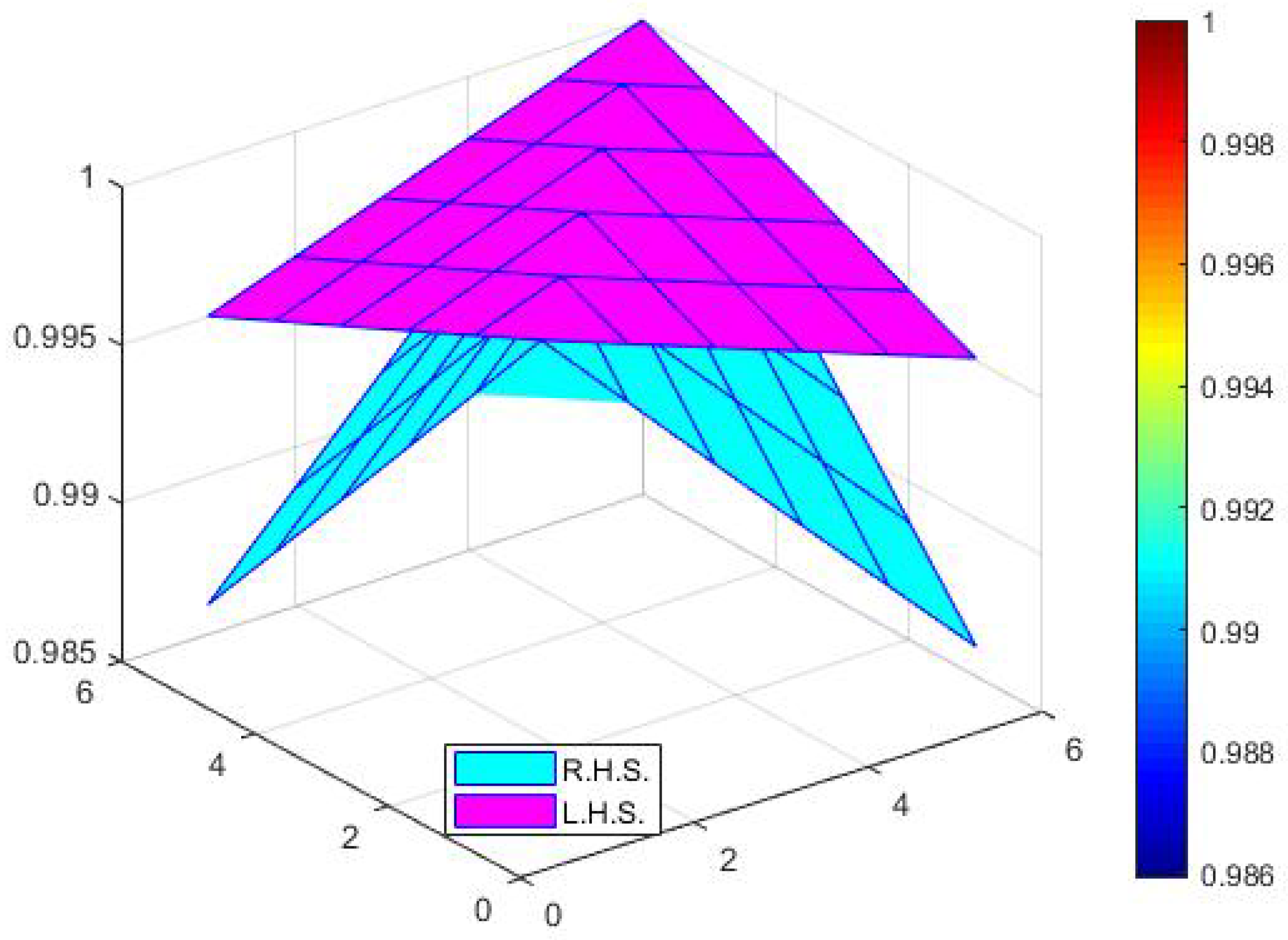
Definition 12. 

Suppose V and X are closed nonempty subsets of an FBMS $\left(C,D,\mathrm{\Lambda },\circ \right)$. We say that $V\cup X$ is approximately compact (in short, AC) with respect to $C\cup D$, if every BS $\left\{{x^o}_n\right\}$ in $V\cup X$ satisfies the following:

$$\mathrm{\Lambda }\left(s^o,{x^o}_n,\tau \right)\to \mathrm{\Lambda }\left(s^o,V\cup X,\tau \right)$$

for some $s\in C\cup D$, which has a BC sub-sequence.

Definition 13. 

Suppose V and X are closed nonempty subsets of an FBMS $\left(C,D,\mathrm{\Lambda },\circ \right)$. An element ${s^o}^{*}\in$$V\cap X$ is called a BPP of the mapping $R:C\cup D\to V\cup X$, if it holds the equation

$$\mathrm{\Lambda }\left({s^o}^{*},R{s^o}^{*},\tau \right)=\mathrm{\Lambda }\left(\left(C\cup D\right),\left(V\cup X\right),\tau \right).$$

Example 3. 

From above Example 2, we have to find BPP

$$\mathrm{\Lambda }\left(0,R\left(0\right),\tau \right)=\mathrm{\Lambda }\left(0,0,\tau \right)=\mathrm{\Lambda }\left(\left(C\cup D\right),\left(V\cup X\right),\tau \right).$$

Hence, 0 is the BPP.

Definition 14. 

Suppose V and X are non-empty, closed subsets of an FBMS $\left(C,D,\mathrm{\Lambda },\circ \right)$. A mapping $R:C\cup D\to V\cup X$ is said to be proximal contraction (in short, PC) on BMS if there exists a real number $a\in \left(0,1\right)$ such that

$$\begin{array}{ccc}\hfill \mathrm{\Lambda }\left({s^o}_1,R{x^o}_1,\tau \right)& =& \mathrm{\Lambda }\left(C\cup D,V\cup X,\tau \right),\hfill \\ \hfill \mathrm{\Lambda }\left({s^o}_2,R{x^o}_2,\tau \right)& =& \mathrm{\Lambda }\left(C\cup D,V\cup X,\tau \right),\hfill \end{array}$$

$$\mathrm{\Lambda }\left({s^o}_1,{s^o}_2,a\tau \right)\ge \left(\mathrm{\Lambda }\left({x^o}_1,{x^o}_2,\tau \right)\right)$$

(1)

for all ${s^o}_1$, ${s^o}_2$, ${x^o}_1$, ${x^o}_2\in C\cup D.$

Example 4. 

Let $C=\left[0,4\right]$ and $D=\left[0,6\right]$ be equipped with $\mathrm{\Lambda }\left({s^o}_1,{s^o}_2,\tau \right)=e^{-\frac{\mid {s^o}_1-{s^o}_2\mid }{\tau }}$ for all ${s^o}_1\in C$ and ${s^o}_2\in D$. Then, $\left(C,D,\mathrm{\Lambda },\circ \right)$ is an FBMS with CTN ${s^o}_1\circ {s^o}_2={s^o}_1{s^o}_2$. Let $V=\left[-1,6\right],X=\left[-2,9\right]$ and define the mapping $R:C\cup D\to V\cup X$ by $R\left(s^o\right)=\frac{s^o}{3}$ for $s^o\in C\cup D$. Thus, $\mathrm{\Lambda }\left(C\cup D,V\cup X,\tau \right)=1$, ${\left(C\cup D\right)}_0\subset C\cup D$ and ${\left(V\cup X\right)}_0\subset V\cup X$. Consider, ${s^o}_1=1,{x^o}_1=3$, and ${s^o}_2=2,{x^o}_2=6$, and $a=0.5$

$$\begin{array}{ccc}\hfill \mathrm{\Lambda }\left(1,R3,1\right)& =& \mathrm{\Lambda }\left(C\cup D,V\cup X,1\right),\hfill \\ \hfill \mathrm{\Lambda }\left(2,R6,1\right)& =& \mathrm{\Lambda }\left(C\cup D,V\cup X,1\right),\hfill \end{array}$$

$$\begin{array}{ccc}\hfill \mathrm{\Lambda }\left(1,2,\left(0.5\right)1\right)& \ge & \mathrm{\Lambda }\left(3,6,1\right),\hfill \\ \hfill 0.1353& \ge & 0.0498.\hfill \end{array}$$

Hence, R is a PC.

Definition 15. 

Suppose V and X are closed nonempty subsets of an FBMS $\left(C,D,\mathrm{\Lambda },\circ \right)$. A mapping $R:C\cup D\to V\cup X$ is said to be Reich–Rus–Ciric type IPC, if there exists a real number $a\in [0,1)$ and $\alpha ,\beta \in \left(0,1\right)$ such that

$$\begin{array}{ccc}\hfill \mathrm{\Lambda }\left({s^o}_1,R{x^o}_1,\tau \right)& =& \mathrm{\Lambda }\left(C\cup D,V\cup X,\tau \right),\hfill \\ \hfill \mathrm{\Lambda }\left({s^o}_2,R{x^o}_2,\tau \right)& =& \mathrm{\Lambda }\left(C\cup D,V\cup X,\tau \right),\hfill \end{array}$$

$$\mathrm{\Lambda }\left({s^o}_1,{s^o}_2,a\tau \right)\ge {\left[\mathrm{\Lambda }\left({x^o}_1,{x^o}_2,\tau \right)\right]}^{\alpha }{\left[G\left({x^o}_1,{s^o}_1,\tau \right)\right]}^{\beta }{\left[\mathrm{\Lambda }\left({x^o}_2,{s^o}_2,\tau \right)\right]}^{1-\alpha -\beta },$$

(2)

for all ${s^o}_1$, ${s^o}_2$, ${x^o}_1$, ${x^o}_2\in C\cup D$.

Example 5. 

Let $C=\left[0,4\right]$ and $D=\left[0,6\right]$ be equipped with $\mathrm{\Lambda }\left({s^o}_1,{s^o}_2,\tau \right)={\displaystyle \frac{\tau }{\tau +\mid {s^o}_1-{s^o}_2\mid }}$ for all ${s^o}_1\in C$ and ${s^o}_2\in D$. Then, $\left(C,D,\mathrm{\Lambda },\circ \right)$ is an FBMS with CTN ${s^o}_1\circ {s^o}_2={s^o}_1{s^o}_2$. Let $V=\left[-1,6\right],X=\left[-2,9\right]$ and define the mapping $R:C\cup D\to V\cup X$ by $R\left(s^o\right)=\frac{s^o}{2}$ for $s^o\in C\cup D$. Thus, $\mathrm{\Lambda }\left(C\cup D,V\cup X,\tau \right)=1$, ${\left(C\cup D\right)}_0\subset C\cup D$ and ${\left(V\cup X\right)}_0\subset V\cup X$. Consider, ${s^o}_1=1,{x^o}_1=2$, and ${s^o}_2=2,{x^o}_2=4$, and $a=0.7$

$$\begin{array}{ccc}\hfill \mathrm{\Lambda }\left(1,R2,1\right)& =& \mathrm{\Lambda }\left(C\cup D,V\cup X,1\right),\hfill \\ \hfill \mathrm{\Lambda }\left(2,R4,1\right)& =& \mathrm{\Lambda }\left(C\cup D,V\cup X,1\right),\hfill \end{array}$$

$$\begin{array}{ccc}\hfill G\left(1,2,\left(0.7\right)1\right)& \ge & \mathrm{\Lambda }{\left(2,4,1\right)}^{\frac{1}{2}}\mathrm{\Lambda }{\left(2,1,1\right)}^{\frac{1}{3}}\mathrm{\Lambda }{\left(4,2,1\right)}^{1-\frac{1}{2}-\frac{1}{3}},\hfill \\ \hfill 0.4118& \ge & 0.3815.\hfill \end{array}$$

Similarly, this holds for all other cases, as shown in Figure 1. Hence, R is a Reich–Rus–Ciric type IPC.

Definition 16. 

Suppose V and X are non-empty, closed subsets of an FBMS $\left(C,D,\mathrm{\Lambda },\circ \right)$. A mapping $R:C\cup D\to V\cup X$ is said to be Kannan type IPC, if there exists a real number $a\in [0,1)$ and $\alpha \in \left(0,1\right)$ such that

$$\begin{array}{ccc}\hfill \mathrm{\Lambda }\left({s^o}_1,R{x^o}_1,\tau \right)& =& \mathrm{\Lambda }\left(C\cup D,V\cup X,\tau \right),\hfill \\ \hfill \mathrm{\Lambda }\left({s^o}_2,R{x^o}_2,\tau \right)& =& \mathrm{\Lambda }\left(C\cup D,V\cup X,\tau \right),\hfill \end{array}$$

$$\mathrm{\Lambda }\left({s^o}_1,{s^o}_2,a\tau \right)\ge {\left[\mathrm{\Lambda }\left({x^o}_1,{s^o}_1,\tau \right)\right]}^{\alpha }{\left[\mathrm{\Lambda }\left({x^o}_2,{s^o}_2,\tau \right)\right]}^{1-\alpha },$$

(3)

for all ${s^o}_1$, ${s^o}_2$, ${x^o}_1$, ${x^o}_2\in C\cup D$.

Example 6. 

Let $C=\left[0,6\right]$, and $D=\left[0,9\right]$ be equipped with $\mathrm{\Lambda }\left({s^o}_1,{s^o}_2,\tau \right)=e^{-\frac{\mid {s^o}_1-{s^o}_2\mid }{\tau }}$ for all ${s^o}_1\in C$ and ${s^o}_2\in D$. Then, $\left(C,D,G,\circ \right)$ is an FBMS with CTN ${s^o}_1\circ {s^o}_2={s^o}_1{s^o}_2$. Let $V=\left[-1,6\right],X=\left[-2,10\right]$ and define the mapping $R:C\cup D\to V\cup X$ by $R\left(s^o\right)=\sqrt{s^o}$ for $s^o\in C\cup D$. Thus, $\mathrm{\Lambda }\left(C\cup D,V\cup X,\tau \right)=1$, ${\left(C\cup D\right)}_0\subset C\cup D$ and ${\left(V\cup X\right)}_0\subset V\cup X$. Consider, ${s^o}_1=2,{x^o}_1=4$, and ${s^o}_2=3,{x^o}_2=9$, and $a=0.5$

$$\begin{array}{ccc}\hfill \mathrm{\Lambda }\left(2,R4,1\right)& =& \mathrm{\Lambda }\left(C\cup D,V\cup X,1\right),\hfill \\ \hfill \mathrm{\Lambda }\left(3,R9,1\right)& =& \mathrm{\Lambda }\left(C\cup D,V\cup X,1\right),\hfill \end{array}$$

$$\begin{array}{ccc}\hfill \mathrm{\Lambda }\left(2,3,\left(0.9\right)1\right)& \ge & \mathrm{\Lambda }{\left(2,1,1\right)}^{\frac{1}{2}}G{\left(9,3,1\right)}^{1-\frac{1}{2}},\hfill \\ \hfill 0.1353& \ge & 0.0179.\hfill \end{array}$$

Hence, R is a Kannan type IPC.

3.1. $\left(\mathrm{{\rm Y}},\mathrm{\Omega }\right)$-Proximal Contraction

This section applies the prior findings of [12,13,19] to the framework of the $\left(\mathrm{{\rm Y}},\mathrm{\Omega }\right)$-proximal contractions for non-self mappings. This approach is especially useful for dealing with problems involving coupled spaces or interactions between different structures. We use $\left(\mathrm{{\rm Y}},\mathrm{\Omega }\right)$-proximal contractions to provide novel convergence and stability criteria for iterative algorithms in such situations, guaranteeing their robustness and efficiency.

Definition 17. 

Suppose V and X is a non-empty, closed subset of an FBMS $\left(C,D,\mathrm{\Lambda },\circ \right)$. A mapping $R:C\cup D\to V\cup X$ is said to be $\left(\mathrm{{\rm Y}},\mathrm{\Omega }\right)$-proximal contraction if

$$\begin{array}{ccc}\hfill G\left({s^o}_1,R{x^o}_1,\tau \right)& =& \mathrm{\Lambda }\left(C\cup D,V\cup X,\tau \right),\hfill \\ \hfill \mathrm{\Lambda }\left({s^o}_2,R{x^o}_2,\tau \right)& =& \mathrm{\Lambda }\left(C\cup D,V\cup X,\tau \right),\hfill \end{array}$$

which implies

$$\mathrm{{\rm Y}}\left(\mathrm{\Lambda }\left({s^o}_1,{s^o}_2,\tau \right)\right)\ge \mathrm{\Omega }\left(\mathrm{\Lambda }\left({x^o}_1,{x^o}_2,\tau \right)\right),$$

(4)

for all ${s^o}_1$, ${s^o}_2$, ${x^o}_1$, ${x^o}_2\in C\cup D$ with ${s^o}_1\ne {s^o}_2,$ and $\tau >0$ where, $\left(\mathrm{{\rm Y}},\mathrm{\Omega }\right):(0,1]\to \mathbb{R}$ are two function such that $\mathrm{{\rm Y}}\left(s\right)<\mathrm{\Omega }\left(s^o\right)$ for $s^o\in (0,1].$

The following example shows that $\left(\mathrm{{\rm Y}},\mathrm{\Omega }\right)$ is PC.

Example 7. 

Let $C=\left[0,6\right]$ and $D=\left[0,10\right]$ be equipped by $\mathrm{\Lambda }\left({s^o}_1,{s^o}_2,\tau \right)=\frac{\tau }{\tau +\mid {s^o}_1-{s^o}_2\mid }$ for all ${s^o}_1\in C$ and ${s^o}_2\in D$. Then, $\left(C,D,\mathrm{\Lambda },\circ \right)$ is an FBMS, with CTN ${s^o}_1\circ {s^o}_2={s^o}_1{s^o}_2$. Let $V=\left[-1,12\right],X=\left[-2,15\right]$ and define the mapping $R:C\cup D\to V\cup X$ by $R\left(s^o\right)={s^o}^2$ for $s^o\in C\cup D$. Thus, $\mathrm{\Lambda }\left(C\cup D,V\cup X,\tau \right)=1$, ${\left(C\cup D\right)}_0\subset C\cup D$ and ${\left(V\cup X\right)}_0\subset V\cup X$. Then clearly, $R\left({\left(C\cup D\right)}_0\right)\subseteq {\left(V\cup X\right)}_0$. The functions $\mathrm{{\rm Y}}\left(s^o\right)$ and $\mathrm{\Omega }\left(s^o\right)$ are defined as follows:

$$\begin{array}{cc}\hfill \mathrm{{\rm Y}}\left(s^o\right)=\left\{\begin{array}{cc}\frac{1}{ln{s}^o},\hfill & for0<s^o<1,\hfill \\ 1,\hfill & for{s}^o=1.\hfill \end{array}\right.& \mathrm{\Omega }\left(s^o\right)=\left\{\begin{array}{cc}\frac{1}{ln\left({s^o}^2\right)},\hfill & for0<s^o<1,\hfill \\ 2,\hfill & for{s}^o=1.\hfill \end{array}\right.forall{s}^o\in (0,1].\end{array}$$

Hence, R is a $\left(\mathrm{{\rm Y}},\mathrm{\Omega }\right)$-PC. Moreover, the other requirements of the definition (4) are satisfied. Then, 0 is a BPP of the mapping R. Consider, ${s^o}_1=4$, ${s^o}_2=9$ and ${x^o}_1=2$, ${x^o}_2=3$, $\tau =1$ and $a=\frac{1}{6}$; then,

$$\begin{array}{ccc}\hfill \mathrm{\Lambda }\left(4,R2,1\right)& =& \mathrm{\Lambda }\left(C\cup D,V\cup X,1\right),\hfill \\ \hfill \mathrm{\Lambda }\left(9,R3,1\right)& =& \mathrm{\Lambda }\left(C\cup D,V\cup X,1\right),\hfill \end{array}$$

which implies that

$$\begin{array}{ccc}\hfill \mathrm{\Lambda }\left(4,9,\frac{1}{6}\left(1\right)\right)& \ge & \left(\mathrm{\Lambda }\left(2,3,1\right)\right),\hfill \\ \hfill \frac{\frac{1}{6}}{\frac{1}{6}+\mid 4-9\mid }& \ge & {\displaystyle \frac{1}{1+1}},\hfill \\ \hfill 0.0322& \ge & 0.5,\hfill \end{array}$$

which is a contradiction. Hence, R is not a PC without $\left(\mathrm{{\rm Y}},\mathrm{\Omega }\right)$.

Lemma 1. 

Let $\left(C,D,\mathrm{\Lambda },\circ \right)$ be an FBMS and $\left\{{s^o}_n,{x^o}_n\right\}$ be a BS in $E\cup F$ that is not Cauchy BS and ${lim}_{n\to \infty }\mathrm{\Lambda }\left({s^o}_n,{x^o}_{n+1},\tau \right)=1$. Then, there exists $ϵ>0$ and two bisubsequences $\left\{{s^o}_{n_k}\right\}$ and $\left\{{s^o}_{m_k}\right\}$ of $\left\{{s^o}_n\right\}$ such that

$$\underset{k\to \infty }{lim}\mathrm{\Lambda }\left({s^o}_{n_k+1},{x^o}_{m_k+1},\tau \right)=ϵ+,$$

(5)

$$\underset{k\to \infty }{lim}\mathrm{\Lambda }\left({s^o}_{n_k},{x^o}_{m_k},\tau \right)=\underset{k\to \infty }{lim}\mathrm{\Lambda }\left({s^o}_{n_k+1},{x^o}_{m_k},\tau \right)=\underset{k\to \infty }{lim}\mathrm{\Lambda }\left({s^o}_{n_k},{x^o}_{m_k+1},\tau \right)=ϵ.$$

(6)

Proof. 

Since $\left\{s_n,{x^o}_n\right\}$ is not a Cauchy bi-sequence and ${lim}_{n\to \infty }G\left({s^o}_n,{x^o}_n,\tau \right)=1$, there exists for $ϵ>0$ and $n_0\ge 1$ such that for each $n>n_0$ there exists $n,m>n_0$ such that $n\ge m$

$$\mathrm{\Lambda }\left({s^o}_{n+1},{x^o}_{m+1},\tau \right)>ϵ\mathrm{and}\mathrm{\Lambda }\left({s^o}_{n+1},{x^o}_n,\tau \right)\le ϵ.$$

Thus, we can make two subsequences of $\left\{{x^o}_{n_k}\right\}$ and $\left\{{x^o}_{m_k}\right\}$ of $\left\{{x^o}_n\right\}$ such that

$$\mathrm{\Lambda }\left({s^o}_{n_k+1},{x^o}_{m_k+1},\tau \right)>ϵ\mathrm{and}\mathrm{\Lambda }\left({s^o}_{n_k+1},{x^o}_{m_k},\tau \right)\le ϵ.$$

From these inequalities and triangular inequality, we obtain

$$ϵ<\mathrm{\Lambda }\left({s^o}_{n_k+1},{x^o}_{m_k+1},\tau \right)\ge \mathrm{\Lambda }\left({s^o}_{n_k+1},{x^o}_{n_k},\tau \right)\circ \mathrm{\Lambda }\left({x^o}_{n_k},{x^o}_{m_k},\tau \right)\circ \mathrm{\Lambda }\left({x^o}_{m_k},{x^o}_{m_k+1},\tau \right)\ge ϵ\mathrm{\Lambda }\left({x^o}_{m_k},{x^o}_{m_k+1},\tau \right).$$

By the Sandwich theorem, we obtain (5). Furthermore, we have

$${\displaystyle \frac{\mathrm{\Lambda }\left({s^o}_{n_k+1},{x^o}_{m_k+1},\tau \right)}{\mathrm{\Lambda }\left({x^o}_{m_k+1},{x^o}_{m_k},\tau \right)}}\ge \mathrm{\Lambda }\left({s^o}_{n_k+1},{x^o}_{n_k},\tau \right)\circ \mathrm{\Lambda }\left({x^o}_{n_k},{x^o}_{m_k},\tau \right)\ge 2ϵ,$$

which implies the second limit (6). From the following two inequalities,

$${\displaystyle \frac{\mathrm{\Lambda }\left({s^o}_{n_k+1},{x^o}_{m_k+1},\tau \right)}{\mathrm{\Lambda }\left({x^o}_{n_k},{x^o}_{n_k+1},\tau \right)}}\ge \mathrm{\Lambda }\left({x^o}_{n_k},{x^o}_{m_k},\tau \right)\circ \mathrm{\Lambda }\left({s^o}_{n_k+1},{x^o}_{m_k+1},\tau \right)\ge ϵ\mathrm{\Lambda }\left({x^o}_{n_k},{x^o}_{n_k+1},\tau \right),$$

$${\displaystyle \frac{ϵ}{\mathrm{\Lambda }\left({s^o}_{n_k},{x^o}_{n_k+1},\tau \right)}}>\mathrm{\Lambda }\left({s^o}_{n_k},{x^o}_{m_k+1},\tau \right)\circ \mathrm{\Lambda }\left({x^o}_{n_k},{x^o}_{m_k},\tau \right)\ge \mathrm{\Lambda }\left({x^o}_{n_k+1},{x^o}_{m_k+1},\tau \right)\circ \mathrm{\Lambda }\left({x^o}_{n_k},{x^o}_{n_k+1},\tau \right),$$

we deduce the first and third limits in (6). □

Lemma 2. 

Let $\mathrm{\Omega }:(0,1]\to \mathbb{R}$. Then the following axioms are equivalent:

(i) 

$\underset{s^o>ϵ}{inf}\mathrm{\Omega }\left(s^o\right)>-\infty$ for every $ϵ>0;$

(ii) 

$\underset{s^o\to ϵ+}{lim}sup\mathrm{\Omega }\left(s^o\right)>-\infty$ for every $ϵ>0;$

(iii) 

${lim}_{n\to \infty }\mathrm{\Omega }\left({s^o}_n\right)=-\infty$ implies that ${lim}_{n\to \infty }\left({s^o}_n\right)=0.$

Proof. 

(i) ⇒ (ii): Assume that condition (i) holds and that $\underset{s^o>ϵ}{inf}\mathrm{\Omega }\left(s^o\right)=s^o$ for some $ϵ>0$. This implies that $\mathrm{\Omega }\left(s^o\right)\ge s^o$ for all $s^o>ϵ$. Since $lim\underset{s^o\to ϵ}{inf}\mathrm{\Omega }\left(s^o\right)\ge s^o$ it follows that condition (ii) is satisfied.

(ii) ⇒ (iii): Let us assume that condition (ii) is valid and that ${lim}_{n\to \infty }\mathrm{\Omega }\left({s^o}_n\right)=-\infty$ for a sequence $\left({s^o}_n\right)\subseteq \left(0,\infty \right)$. Suppose ${s^o}_n$ does not tend to zero. There exists $ϵ>0$ and a subsequence $\left({s^o}_{n_k}\right)$ such that ${s^o}_{n_k}>ϵ$ for all $k\ge 1$. Given that ${lim}_{n\to \infty }\mathrm{\Omega }\left({s^o}_n\right)=-\infty$ it follows that ${lim}_{k\to \infty }\mathrm{\Omega }\left({s^o}_{n_k}\right)=-\infty$ contradicting condition (ii). Consequently, we obtain ${lim}_{n\to \infty }{s^o}_n=0$ proving that (iii) holds.

(iii) ⇒ (i): Suppose condition (iii) is true and assume for contradiction that $\underset{s^o>ϵ}{inf}\mathrm{\Omega }\left(s^o\right)=-\infty$ for some $ϵ>0$. So there must exist a subsequence $\left({s^o}_n\right)\subseteq \left(0,\infty \right)$ such that ${s^o}_n>ϵ$ for all $n\ge 1$ and ${lim}_{n\to \infty }\mathrm{\Omega }\left({s^o}_n\right)=-\infty$. By condition (iii) that is ${lim}_{n\to \infty }{s^o}_n=0$ this contradicts the assumption that ${s^o}_n>ϵ$. Therefore the condition (i) must be hold. □

Lemma 3. 

Let $\{s_n^o,{x^o}_n\}$ be a BS in $\left(C,D,\mathrm{\Lambda },\circ \right)$ such that ${lim}_{n\to \infty }\mathrm{\Lambda }({s^o}_n,{x^o}_{n+1},\tau )=1$ and $R:C\cup D\to V\cup X$ be a mapping satisfying (4). If the functions $\mathrm{{\rm Y}},\mathrm{\Omega }:(0,1]\to \mathbb{R}$ are such that

(1) 

$lim{sup}_{s^o\to ϵ+}\mathrm{\Omega }\left(s^o\right)>\mathrm{{\rm Y}}(\in +)$ for any $ϵ>0.$

Then $\{{s^o}_n,{x^o}_n\}$ is CBS.

Proof. 

Suppose that the BS $\{{s^o}_n,{x^o}_n\}$ is not CBS, then by Lemma 1, there exist two bi subsequences $\left\{{s^o}_{n_k}\right\}$, $\left\{{x^o}_{m_k}\right\}$ of $\{{s^o}_n,{x^o}_n\}$ and $ϵ>0$ such that the Equations (5) and (6) hold. By (5), we obtain that $\mathrm{\Lambda }({s^o}_{n_k+1},{x^o}_{m_k+1},\tau )>ϵ$. Since, for ${x^o}_{n_k},{x^o}_{m_k},{s^o}_{m_k+1},{s^o}_{n_k+1}\in C\cup D$, we have

$$\begin{array}{ccc}\hfill \mathrm{\Lambda }({s^o}_{n_k+1},R\left({x^o}_{m_k}\right),\tau )& =& \mathrm{\Lambda }(C\cup D,V\cup X,\tau ),\hfill \\ \hfill \mathrm{\Lambda }({s^o}_{m_k+1},R\left({x^o}_{n_k}\right),\tau )& =& \mathrm{\Lambda }(C\cup D,V\cup X,\tau ),\mathrm{for}\mathrm{all}k\ge 1,\hfill \end{array}$$

thus, by (4), we have

$$\mathrm{{\rm Y}}\left(\mathrm{\Lambda }({s^o}_{n_k+1},{s^o}_{m_k+1},\tau )\right)\ge \mathrm{\Omega }\left(\mathrm{\Lambda }({x^o}_{n_k},{x^o}_{m_k},\tau )\right),\mathrm{for}\mathrm{any}k\ge 1.$$

For if $a_k=\mathrm{\Lambda }({s^o}_{n_k+1},{s^o}_{m_k+1},\tau )$ and $b_k=\mathrm{\Lambda }({s^o}_{n_k},{s^o}_{m_k},\tau )$, we have

$$\mathrm{{\rm Y}}\left(a_k\right)\ge \mathrm{\Omega }\left(b_k\right),\mathrm{for}\mathrm{any}k\ge 1.$$

(7)

By (5) and (6), we have ${lim}_{k\to \infty }{a}_k=ϵ+$ and ${lim}_{k\to \infty }{b}_k=ϵ$. By (7), we obtain that

$$\mathrm{{\rm Y}}(ϵ+)=\underset{k\to \infty }{lim}\mathrm{{\rm Y}}\left(a_k\right)\ge lim\underset{k\to \infty }{sup}\mathrm{\Omega }\left(b_k\right)\ge lim\underset{x^o\to ϵ}{sup}\mathrm{\Omega }\left(x^o\right).$$

(8)

This is conflicted with the axioms (1). Consequently, $\{{s^o}_n,{x^o}_n\}$ is a CBS in $C\cup D$. □

Now, we present the main results.

Theorem 1. 

Suppose V and X are nonempty closed subsets of a CFBMS $\left(C,D,\mathrm{\Lambda },\circ \right),$ such that $V\cup X$ is AC with respect to $C\cup D$. A mapping $R:C\cup D\to V\cup X$ is a $\left(\mathrm{{\rm Y}},\mathrm{\Omega }\right)$-PC if

(i) 

$\mathrm{{\rm Y}}$ is a nondecreasing function, and $lim{sup}_{s^o\to ϵ+}\mathrm{\Omega }\left(s^o\right)>\mathrm{{\rm Y}}(\in +)$ for any $ϵ>0.$

(ii) 

${\left(C\cup D\right)}_0$ is a nonempty subset of $C\cup D$ such that $R{\left(C\cup D\right)}_0\subseteq {\left(V\cup X\right)}_0.$

Then, R has a BPP.

Proof. 

Suppose that ${s^o}_0\in {\left(C\cup D\right)}_0$. Since $R{\left(s^o\right)}_0\in R{\left(C\cup D\right)}_0\subseteq {\left(V\cup X\right)}_0$, then ∃${s^o}_1\in {\left(C\cup D\right)}_0$ such that

$$\mathrm{\Lambda }\left({s^o}_1,R{s^o}_0,\tau \right)=\mathrm{\Lambda }\left(C\cup D,V\cup X,\tau \right).$$

Similarly, since $R\left(s_1\right)\in R{\left(C\cup D\right)}_0\subseteq {\left(C\cup D,V\cup X\right)}_0$, ∃${s^o}_2\in {\left(C\cup D\right)}_0$ such that

$$\mathrm{\Lambda }\left({s^o}_2,R{s^o}_1,\tau \right)=\mathrm{\Lambda }\left(C\cup D,V\cup X,\tau \right).$$

During this process, we establish a BS $\left\{{s^o}_n\right\}\in {\left(C\cup D\right)}_0$ such that

$$\mathrm{\Lambda }\left({s^o}_{n+1},R{s^o}_n,\tau \right)=\mathrm{\Lambda }\left(C\cup D,V\cup X,\tau \right)\forall n\in \mathbb{N}.$$

(9)

If ${s^o}_n={s^o}_{n+1}$, then from (9), obviously, ${s^o}_n$ is a BPP of the mapping R. Consider, ${s^o}_n\ne {s^o}_{n+1}$ for all $n\in \mathbb{N}$, then

$$\mathrm{\Lambda }\left({s^o}_n,R{s^o}_{n-1},\tau \right)=\mathrm{\Lambda }\left(C\cup D,V\cup X,\tau \right)$$

and

$$\mathrm{\Lambda }\left({s^o}_{n+1},R{s^o}_n,\tau \right)=\mathrm{\Lambda }\left(C\cup D,V\cup X,\tau \right)\forall n\ge 1.$$

Then by using (4), we have

$$\mathrm{{\rm Y}}\left(\mathrm{\Lambda }\left({s^o}_{n+1},{s^o}_n,\tau \right)\right)\ge \mathrm{\Omega }\left(G\left({s^o}_{n-1},{s^o}_n,\tau \right)\right)\mathrm{for}\mathrm{all}{s^o}_{n-1},{s^o}_n,{s^o}_{n+1}\in \left(C\cup D\right).$$

Letting $a_n=\mathrm{\Lambda }({s^o}_{n+1},{s^o}_n,\tau )$, we have

$$\mathrm{{\rm Y}}\left(a_n\right)\ge \mathrm{\Omega }\left(a_{n-1}\right)>\mathrm{{\rm Y}}\left(a_{n-1}\right).$$

(10)

$\mathrm{{\rm Y}}$ is nondecreasing, so by (10), we have $a_n>a_{n-1}$∀$n\in \mathbb{N}$. Hence, the BS $\left\{a_n\right\}$ is positive and strictly decreasing (in short, PASD). Thus, it converges to some element $\gamma \ge 1$ such that ${lim}_{n\to \infty }\mathrm{\Lambda }\left({s^o}_{n+1},{s^o}_n,\tau \right)=\gamma$. Now, from (10) we obtain the following

$$\mathrm{{\rm Y}}\left(a+\right)=\underset{n\to \infty }{lim}\mathrm{{\rm Y}}\left(a_n\right)\ge \underset{n\to \infty }{lim}\mathrm{\Omega }\left(a_{n-1}\right)\ge \underset{x^o\to a+}{lim}sup\mathrm{\Omega }\left(x^o\right).$$

Hence, from supposition (i), it is conflicted thus, $a=1$ and ${lim}_{n\to \infty }\mathrm{\Lambda }\left({s^o}_n,{s^o}_{n+1},\tau \right)=1$. Now, from supposition (i) and Lemma 3, we wind up with the BS $\left\{s_n\right\}$ being a CBS in $\left(C\cup D\right)$.

Since $\left(C,D,\mathrm{\Lambda },\circ \right)$ is a CFBMS, then BS $\left({s^o}_n\right)$ converges, thus BC to a point ${s^o}^{*}\in \left(C\cap D\right)$ such that ${s^o}_n\to {s^o}^{*}$. From Equation (9),

$$\begin{array}{ccc}\hfill \mathrm{\Lambda }\left({s^o}^{*},V\cup X,\tau \right)& \ge & \mathrm{\Lambda }\left({s^o}^{*},R{s^o}_n,\tau \right)\hfill \\ & \ge & \mathrm{\Lambda }\left({s^o}^{*},{s^o}_{n+1},\tau \right)\circ \mathrm{\Lambda }\left({s^o}_n,R{s^o}_n,\tau \right)\circ \mathrm{\Lambda }\left({s^o}_n,{s^o}_{n+1},\tau \right)\hfill \\ & =& \mathrm{\Lambda }\left({s^o}^{*},{s^o}_{n+1},\tau \right)\circ \mathrm{\Lambda }\left(C\cup D,V\cup X,\tau \right)\circ \mathrm{\Lambda }\left({s^o}^{*},{s^o}_{n+1},\tau \right).\hfill \end{array}$$

Therefore, $\mathrm{\Lambda }\left({s^o}^{*},R{s^o}_n,\tau \right)\to \mathrm{\Lambda }\left({s^o}^{*},V\cup X,\tau \right)$ as $n\to \infty$. Since $V\cup X$ is AC with respect to $C\cup D$, there exists a subsequence $\left\{R{s^o}_{n_k}\right\}$ of $\left\{R{s^o}_n\right\}$ such that $R{s^o}_{n_k}\to {x^o}^{*}\in V\cap X$ as $k\to \infty$. Therefore, by taking $k\to \infty$ in

$$\mathrm{\Lambda }\left({s^o}_{n_k+1},R{s^o}_{n_k},\tau \right)=\mathrm{\Lambda }\left(C\cup D,V\cup X,\tau \right),$$

(11)

we have

$$\mathrm{\Lambda }\left({s^o}^{*},{x^o}^{*},\tau \right)=\mathrm{\Lambda }\left(C\cup D,V\cup X,\tau \right).$$

Since ${s^o}^{*}\in {\left(C\cup D\right)}_0$. Furthermore, since $R\left({s^o}^{*}\right)\in R\left({\left(C\cup D\right)}_0\right)\subseteq {\left(V\cup X\right)}_0$, there exists $\xi \in {\left(C\cup D\right)}_0$ such that

$$\mathrm{\Lambda }\left(\xi ,R\left({s^o}^{*}\right),\tau \right)=\mathrm{\Lambda }\left(C\cup D,V\cup X,\tau \right).$$

(12)

Suppose that ${s^o}^{*}\ne {s^o}_n$∀$n\in \mathbb{N}$. There exists subsequences $\left\{{s^o}_{m_k}\right\}$ of $\left\{{s^o}_n\right\}$ such that ${s^o}^{*}\ne {s^o}_{m_k}\forall$$k\in \mathbb{N}$. Now, from (11), (12), and the inequality (4), we obtain that

$$\mathrm{{\rm Y}}\left(\mathrm{\Lambda }\left({s^o}_{n_k+1},\xi ,\tau \right)\right)\ge \mathrm{\Omega }\left(\mathrm{\Lambda }\left({s^o}_{n_k},{s^o}^{*},\tau \right)\right)>\mathrm{{\rm Y}}\left(\mathrm{\Lambda }\left({s^o}_{n_k},{s^o}^{*},\tau \right)\right)\mathrm{for}\mathrm{all}k\in \mathbb{N}.$$

Since $\mathrm{{\rm Y}}$ is a nondecreasing function (in short, ND), we have

$$\mathrm{\Lambda }\left({s^o}_{n_k+1},\xi ,\tau \right)>G\left({s^o}_{n_k},{s^o}^{*},\tau \right)$$

for all $k\in \mathbb{N}$. Thus, letting $k\to \infty$, we have $G\left({s^o}^{*},\xi ,\tau \right)=1$ or ${s^o}^{*}=\xi$. Finally, by (12), we have

$$G\left({s^o}^{*},\xi ,\tau \right)=G\left(C\cup D,V\cup X,\tau \right)$$

Thus, ${s^o}^{*}$ is a BPP of the mapping R. □

Theorem 2. 

Suppose V and X are non-empty, closed subsets of a CFBMS $\left(C,D,\mathrm{\Lambda }\right)$ such that $V\cup X$ is AC with respect to $C\cup D$. A mapping $R:C\cup D\to V\cup X$ is a $\left(\mathrm{{\rm Y}},\mathrm{\Omega }\right)$-Pc if

(i) 

$\mathrm{{\rm Y}}$ is a nondecreasing function, $\left\{\mathrm{{\rm Y}}\left({s^o}_n\right)\right\}$ and $\left\{\mathrm{\Omega }\left({s^o}_n\right)\right\}$ are BC such that ${lim}_{n\to \infty }\mathrm{{\rm Y}}\left({s^o}_n\right)={lim}_{n\to \infty }\mathrm{\Omega }\left({s^o}_n\right),$ then the $lim\mathrm{\Lambda }\left({s^o}_n,{s^o}_{n+1},\tau \right)=1.$

(ii) 

${\left(C\cup D\right)}_0$ is a nonempty subset of $\left(C\cup D\right)$ such that $R{\left(C\cup D\right)}_0\subseteq {\left(V\cup X\right)}_0.$

Then, R has a BPP.

Proof. 

Starting with the proof of Theorem 1, we have

$$\mathrm{{\rm Y}}\left(a_n\right)\ge \mathrm{\Omega }\left(a_{n-1}\right)>\mathrm{{\rm Y}}\left(a_{n-1}\right).$$

(13)

By (13), we infer that $\left\{\mathrm{{\rm Y}}\left(a_n\right)\right\}$ is strictly decreasing BS. There are two cases; either the BS $\left\{\mathrm{{\rm Y}}\left(a_n\right)\right\}$ is bounded below or not. If $\left\{\mathrm{{\rm Y}}\left(a_n\right)\right\}$ is not bounded below, then

$$\underset{a_n>ϵ}{inf}\mathrm{{\rm Y}}\left(a_n\right)>-\infty \mathrm{for}\mathrm{every}ϵ>0,n\in \mathbb{N}.$$

From Lemma 2, $a_n\to 1$ as $n\to \infty .$ Secondly, if the BS $\left\{\mathrm{{\rm Y}}\left(a_n\right)\right\}$ is bounded below, then it is BCS. By (13), the BS $\left\{\mathrm{\Omega }\left(a_n\right)\right\}$ is also BC; moreover, both have the same limit. By supposition (i), we have ${lim}_{n\to \infty }{a}_n=1$, or ${lim}_{n\to \infty }\mathrm{\Lambda }\left({s^o}_n,{s^o}_{n+1},\tau \right)=1,$ for any BS $\left\{{s^o}_n\right\}$ in $C\cup D$. The remaining proof of the Theorem is taken the same as the proof of Theorem 1; therefore, we have

$$\mathrm{\Lambda }\left(\xi ,R\left({s^o}^{*}\right),\tau \right)=\mathrm{\Lambda }\left(C\cup D,V\cup X,\tau \right).$$

Hence, ${s^o}^{*}$ is a BPP of the mapping R. □

3.2. $\left(\mathrm{{\rm Y}},\mathrm{\Omega }\right)$-Interpolative Reich–Ciric–Rus Type Proximal Contraction

In this part, we will develop conditions for determining the best proximity point for Reich–Rus–Ciric type contractions and generalize the findings of [17,18,19] to the framework of FBMS. In order to overcome the difficulties caused by nonlinearity and imprecision, we use the dual metrics and fuzzy parameters to construct adequate requirements for the existence and uniqueness of BPP for such contractions. This generalization offers a throughout framework for resolving BPP problems in FBMS by introducing new iterative schemes and convergence studies to consolidate and expand on previous findings.

Definition 18. 

Suppose V and X are closed nonempty subsets of an FBMS $\left(C,D,\mathrm{\Lambda },\circ \right)$. A mapping $R:C\cup D\to V\cup X$ is said to be $\left(\mathrm{{\rm Y}},\mathrm{\Omega }\right)$-Reich–Rus–Ciric type IPC if there exists $\alpha ,\beta \in \left(0,1\right);\alpha +\beta <1$, verifying

$$\begin{array}{ccc}\hfill \mathrm{\Lambda }\left({s^o}_1,R{x^o}_1,\tau \right)& =& \mathrm{\Lambda }\left(C\cup D,V\cup X,\tau \right),\hfill \\ \hfill \mathrm{\Lambda }\left({s^o}_2,R{x^o}_2,\tau \right)& =& \mathrm{\Lambda }\left(C\cup D,V\cup X,\tau \right),\hfill \end{array}$$

which implies

$$\mathrm{{\rm Y}}\left(\mathrm{\Lambda }\left({s^o}_1,{s^o}_2,\tau \right)\right)\ge \mathrm{\Omega }\left({\left(\mathrm{\Lambda }\left({x^o}_1,{x^o}_2,\tau \right)\right)}^{\alpha }{\left(\mathrm{\Lambda }\left({x^o}_1,{s^o}_1,\tau \right)\right)}^{\beta }{\left(G\left({x^o}_2,{s^o}_2,\tau \right)\right)}^{1-\alpha -\beta }\right)$$

(14)

for all ${s^o}_1$, ${s^o}_2$, ${x^o}_1$, ${x^o}_2\in C\cup D$ and $\tau >0$ with ${s^o}_1\ne {s^o}_2,$ where, $\left(\mathrm{{\rm Y}},\mathrm{\Omega }\right):(0,1]\to \mathbb{R}$ are two function such that $\mathrm{{\rm Y}}\left(s^o\right)<\mathrm{\Omega }\left(s^o\right)$ for $s^o\in (0,1].$

Example 8. 

Let $C=\left[0,2\right]$ and $D=\left[0,4\right]$ be equipped with $G\left({s^o}_1,{s^o}_2,\tau \right)=e^{-\frac{\mid {s^o}_1-{s^o}_2\mid }{\tau }}$ for all ${s^o}_1\in C$ and ${s^o}_2\in D$. Then, $\left(C,D,G,\circ \right)$ is an FBMS with CTN ${s^o}_1\circ {s^o}_2={s^o}_1{s^o}_2$. Let $V=\left[-1,4\right],X=\left[-2,8\right]$ and define the mapping $R:C\cup D\to V\cup X$ by $R\left(s^o\right)=2s^o$ for all $s^o\in C\cup D$. Thus, $\mathrm{\Lambda }\left(C\cup D,V\cup X,\tau \right)=1$, ${\left(C\cup D\right)}_0\subset C\cup D$ and ${\left(V\cup X\right)}_0\subset V\cup X$. Then clearly, $R\left({\left(C\cup D\right)}_0\right)\subseteq {\left(V\cup X\right)}_0$. Define the function $\left(\mathrm{{\rm Y}},\mathrm{\Omega }\right):(0,1]\to \mathbb{R}$ by

$$\mathrm{{\rm Y}}\left(s^o\right)=\left\{\begin{array}{cc}{\displaystyle \frac{1}{2^{ln\left(2s^o\right)}}}\hfill & for0<s^o<1,\hfill \\ 1\hfill & for{s}^o=1\hfill \end{array}\right.,\mathrm{\Omega }\left(s^o\right)=\left\{\begin{array}{cc}{\displaystyle \frac{1}{2^{ln\left(s^o\right)}}}\hfill & for0<s^o<1,\hfill \\ 2\hfill & for{s}^o=1\hfill \end{array}\right.forall{s}^o\in (0,1].$$

Hence, R is a $\left(\mathrm{{\rm Y}},\mathrm{\Omega }\right)$ Reich–Rus–Ciric type IPC. Furthermore, the other requirements of the definition (14) are satisfied. Then, 0 is the BPP. Consider, ${s^o}_1=2$, ${x^o}_1=1$, ${s^o}_2=4$, ${x^o}_2=2\in C\cup D$, $\tau =1,a=0.9$, $\alpha =\frac{1}{2}$ and $\beta =\frac{1}{3}.$

$$\begin{array}{ccc}\hfill \mathrm{\Lambda }\left({s^o}_1,R{x^o}_1,\tau \right)& =& 1=\mathrm{\Lambda }\left(C\cup D,V\cup X,\tau \right),\hfill \\ \hfill \mathrm{\Lambda }\left({s^o}_2,R{x^o}_2,\tau \right)& =& 1=\mathrm{\Lambda }\left(C\cup D,V\cup X,\tau \right).\hfill \end{array}$$

This implies that

$$\begin{array}{ccc}\hfill \mathrm{\Lambda }\left({s^o}_1,{s^o}_2,a\tau \right)& \ge & \left({\left(\mathrm{\Lambda }\left({x^o}_1,{x^o}_2,\tau \right)\right)}^{\alpha }{\left(\mathrm{\Lambda }\left({x^o}_1,{s^o}_1,\tau \right)\right)}^{\beta }{\left(\mathrm{\Lambda }\left({x^o}_2,{s^o}_2,\tau \right)\right)}^{1-\alpha -\beta }\right)\hfill \\ \hfill e^{-\frac{2}{0.9}}& \ge & \left(0.6065\right)\left(0.7165\right)\left(0.7165\right)\hfill \\ \hfill 0.1084& \ge & 0.3114,\hfill \end{array}$$

which is a contradiction. Hence, R is not a Reich–Rus–Ciric type IPC.

Theorem 3. 

Suppose V and X are non-empty, closed subsets of a CFBMS $\left(C,D,\mathrm{\Lambda },\circ \right),$ such that $V\cup X$ is AC with respect to $C\cup D$. Suppose a mapping $R:C\cup D\to V\cup X$ is a $\left(\mathrm{{\rm Y}},\mathrm{\Omega }\right)$ Reich–Rus–Ciric type IPC if

(i) $\mathrm{{\rm Y}}$ is nondecreasing, and $lim{sup}_{s^o\to ϵ+}\mathrm{\Omega }\left(s^o\right)>\mathrm{{\rm Y}}(\in +)$ for any $ϵ>0.$

(ii) ${\left(C\cup D\right)}_0$ is a nonempty subset of $C\cup D$ such that $R{\left(C\cup D\right)}_0\subseteq {\left(V\cup X\right)}_0.$

Then R has a BPP.

Proof. 

Taking the same step of Theorem 1, we establish a BS $\left\{{s^o}_n\right\}$ in ${\left(C\cup D\right)}_0$ such that

$$\mathrm{\Lambda }\left({s^o}_{n+1},R{s^o}_n,\tau \right)=\mathrm{\Lambda }\left(C\cup D,V\cup X,\tau \right)\forall n\in \mathbb{N}.$$

(15)

If ${s^o}_n={s^o}_{n+1}$, then from (15), obviously, ${s^o}_n$ is a BPP of the mapping R. Consider, ${s^o}_n\ne {s^o}_{n+1}$ for all $n\in \mathbb{N}$, then

$$\mathrm{\Lambda }\left({s^o}_n,R{s^o}_{n-1},\tau \right)=\mathrm{\Lambda }\left(C\cup D,V\cup X,\tau \right),$$

and

$$\mathrm{\Lambda }\left({s^o}_{n+1},R{s^o}_n,\tau \right)=\mathrm{\Lambda }\left(C\cup D,V\cup X,\tau \right)\forall n\ge 1.$$

Then, by using (14), we have

$$\mathrm{{\rm Y}}\left(G\left({s^o}_{n+1},{s^o}_n,\tau \right)\right)\ge \mathrm{\Omega }\left(\mathrm{\Lambda }{\left({s^o}_{n-1},{s^o}_n,\tau \right)}^{\alpha }{\left(G\left({s^o}_{n-1},{s^o}_n,\tau \right)\right)}^{\beta }{\left(\mathrm{\Lambda }\left({s^o}_n,{s^o}_{n+1},\tau \right)\right)}^{1-\alpha -\beta }\right),$$

(16)

for all distinct ${s^o}_{n-1},{s^o}_n,{s^o}_{n+1}\in C\cup D$. Since $\mathrm{\Omega }\left(s^o\right)>\mathrm{{\rm Y}}\left(s^o\right)$∀$s^o\in \mathbb{R}$, by (16), we have

$$\mathrm{{\rm Y}}\left(\mathrm{\Lambda }\left({s^o}_{n+1},{s^o}_n,\tau \right)\right)>\mathrm{{\rm Y}}\left(\mathrm{\Lambda }{\left({s^o}_{n-1},{s^o}_n,\tau \right)}^{\alpha }{\left(\mathrm{\Lambda }\left({s^o}_{n-1},{s^o}_n,\tau \right)\right)}^{\beta }{\left(\mathrm{\Lambda }\left({s^o}_n,{s^o}_{n+1},\tau \right)\right)}^{1-\alpha -\beta }\right).$$

Since $\mathrm{{\rm Y}}$ is NDF, we have

$$\mathrm{\Lambda }\left({s^o}_{n+1},{s^o}_n,\tau \right)\ge \mathrm{\Lambda }{\left({s^o}_{n-1},{s^o}_n,\tau \right)}^{\alpha +\beta }{\left(\mathrm{\Lambda }\left({s^o}_n,{s^o}_{n+1},\tau \right)\right)}^{1-\alpha -\beta }.$$

This implies that

$$\mathrm{\Lambda }{\left({s^o}_{n+1},{s^o}_n,\tau \right)}^{\alpha +\beta }\ge \mathrm{\Lambda }{\left({s^o}_{n-1},{s^o}_n\right)}^{\alpha +\beta }.$$

This implies that $a_n>a_{n-1}$ for all $n\in \mathbb{N}.$ This shows that the BS $\left\{a_n\right\}$ is PASD. Hence, it converges to some element $\gamma \ge 1$ such that ${lim}_{n\to \infty }\mathrm{\Lambda }\left({s^o}_{n+1},{s^o}_n\right)=\gamma$. Now from (16), we obtain the following

$$\mathrm{{\rm Y}}\left(a+\right)=\underset{n\to \infty }{lim}\mathrm{{\rm Y}}\left(a_n\right)\ge \underset{n\to \infty }{lim}\mathrm{\Omega }\left({\left(a_{n-1}\right)}^{\alpha +\beta }{\left(a_n\right)}^{1-\alpha -\beta }\right)\ge \underset{x^o\to a+}{lim}sup\mathrm{\Omega }\left(x^o\right).$$

This conflicts with supposition (i), hence, $a=1$ and ${lim}_{n\to \infty }\mathrm{\Lambda }\left({s^o}_n,{s^o}_{n+1},\tau \right)=1$. From supposition (i) and Lemma 3, we wind up with the BS $\left\{{s^o}_n\right\}$ being a CBS in $\left(C\cup D\right)$. The remaining proof of the Theorem is taken as the same as the proof of Theorem 1. Hence, we find that ${s^o}^{*}$ is a BPP of the mapping R. □

Theorem 4. 

Suppose V and X are closed non-empty subsets of a CFBMS $\left(C,D,\mathrm{\Lambda },\circ \right),$ such that $V\cup X$ is AC with respect to $C\cup D$. Suppose a mapping $R:C\cup D\to V\cup X$ is a $\left(\mathrm{{\rm Y}},\mathrm{\Omega }\right)$ Reich–Rus–Ciric type IPC if

(i) 

$\mathrm{{\rm Y}}$ is nondecreasing, $\left\{\mathrm{{\rm Y}}\left({s^o}_n\right)\right\}$ and $\left\{\mathrm{\Omega }\left({s^o}_n\right)\right\}$ are convergent BS such that ${lim}_{n\to \infty }\mathrm{{\rm Y}}\left({s^o}_n\right)={lim}_{n\to \infty }\mathrm{\Omega }\left({s^o}_n\right),$ then the $lim\mathrm{\Lambda }\left({s^o}_n,{s^o}_{n+1},\tau \right)=1.$

(ii) 

${\left(C\cup D\right)}_0$ is a nonempty subset of $\left(C\cup D\right)$ such that $R{\left(C\cup D\right)}_0\subseteq {\left(V\cup X\right)}_0.$

Then, R has a BPP.

Proof. 

Chasing the starting steps taken in proof of Theorem 3, we have

$$\mathrm{{\rm Y}}\left(a_n\right)\ge \mathrm{\Omega }\left({\left(a_{n-1}\right)}^{\alpha +\beta }{\left(a_n\right)}^{1-\alpha -\beta }\right)>\mathrm{{\rm Y}}\left({\left(a_{n-1}\right)}^{\alpha +\beta }{\left(a_n\right)}^{1-\alpha -\beta }\right)$$

(17)

Now, the remaining proof is taken the same as the proof of 2. Thus, we obtain ${s^o}^{*}$ is a BPP of the mapping R. □

3.3. $\left(\mathrm{{\rm Y}},\mathrm{\Omega }\right)$-Interpolative Kannan Type Proximal Contraction

In this part, we will determine the BPP of the Kannan type IPC within the context of FBMS. Using the extensive structure of FBMS, we intend to generalize and extend the findings reported in [17,18,19], which mostly concentrate on standard metric spaces or specialized contractive mappings. Furthermore, the proposed constraints guarantee the presence and uniqueness of the BPP.

Definition 19. 

Suppose V and X are non-empty, closed subsets of an FBMS $\left(C,D,\mathrm{\Lambda }\right)$. A mapping $R:C\cup D\to V\cup X$ is said to be $\left(\mathrm{{\rm Y}},\mathrm{\Omega }\right)$-Kannan type IPC if there exists $\alpha \in \left(0,1\right);\alpha +\beta <1$, verifying

$$\begin{array}{ccc}\hfill \mathrm{\Lambda }\left({s^o}_1,R{x^o}_1,\tau \right)& =& \mathrm{\Lambda }\left(C\cup D,V\cup X,\tau \right),\hfill \\ \hfill \mathrm{\Lambda }\left({s^o}_2,R{x^o}_2,\tau \right)& =& \mathrm{\Lambda }\left(C\cup D,V\cup X,\tau \right),\hfill \end{array}$$

which implies

$$\mathrm{{\rm Y}}\left(\mathrm{\Lambda }\left({s^o}_1,{s^o}_2,\tau \right)\right)\ge \mathrm{\Omega }\left({\left(\mathrm{\Lambda }\left({x^o}_1,{s^o}_1,\tau \right)\right)}^{\alpha }{\left(\mathrm{\Lambda }\left({x^o}_2,{s^o}_2,\tau \right)\right)}^{1-\alpha }\right).$$

(18)

for all ${s^o}_1$, ${s^o}_2$, ${x^o}_1$, ${x^o}_2\in C\cup D$ and $\tau >0$ with ${s^o}_1\ne {s^o}_2,$ where $\left(\mathrm{{\rm Y}},\mathrm{\Omega }\right):(0,1]\to \mathbb{R}$ are two function such that $\mathrm{{\rm Y}}\left(s^o\right)<\mathrm{\Omega }\left(s^o\right)$ for $s^o\in (0,1].$

Example 9. 

Let $C=\left[0,8\right]$ and $D=\left[0,10\right]$ be equipped with $\mathrm{\Lambda }\left({s^o}_1,{s^o}_2,\tau \right)=\frac{\tau }{\tau +\mid {s^o}_1-{s^o}_2\mid }$ for all ${s^o}_1\in C$ and ${s^o}_2\in D$. Then, $\left(C,D,\mathrm{\Lambda },\circ \right)$ is an FBMS with CTN ${s^o}_1\circ {s^o}_2={s^o}_1{s^o}_2$. Let $V=\left[-1,12\right],X=\left[-2,14\right]$ and define the mapping $R:C\cup D\to V\cup X$ by $R\left(s^o\right)=\frac{s^o}{4}$ for all $s^o\in C\cup D$. Thus, $\mathrm{\Lambda }\left(C\cup D,V\cup X,\tau \right)=1$, ${\left(C\cup D\right)}_0\subset C\cup D$ and ${\left(V\cup X\right)}_0\subset V\cup X$. Then clearly, $R\left({\left(C\cup D\right)}_0\right)\subseteq {\left(V\cup X\right)}_0$. Define the function $\left(\mathrm{{\rm Y}},\mathrm{\Omega }\right):(0,1]\to \mathbb{R}$ by

$$\mathrm{{\rm Y}}\left(s^o\right)={s^o}^{2}and\mathrm{\Omega }\left(s^o\right)=s^{o}forall{s}^o\in (0,1].$$

Hence, R is a $\left(\mathrm{{\rm Y}},\mathrm{\Omega }\right)$ Kannan type IPC. Furthermore, the other requirements of the definition (18) are held. Therefore, 0 is the BPP of mapping R. Consider, ${s^o}_1=1$, ${x^o}_1=4$, ${s^o}_2=2$, ${x^o}_2=8\in C\cup D,\tau =1$ and $a=0.2$ and $\alpha =\frac{1}{2}$.

$$\begin{array}{ccc}\hfill \mathrm{\Lambda }\left({s^o}_1,R{x^o}_1,\tau \right)& =& 1=\mathrm{\Lambda }\left(C\cup D,V\cup X,\tau \right),\hfill \\ \hfill \mathrm{\Lambda }\left({s^o}_2,R{x}_2,\tau \right)& =& 1=\mathrm{\Lambda }\left(C\cup D,V\cup X,\tau \right).\hfill \end{array}$$

This implies that

$$\begin{array}{ccc}\hfill \mathrm{\Lambda }\left({s^o}_1,{s^o}_2,a\tau \right)& \ge & \left({\left(\mathrm{\Lambda }\left({x^o}_1,{s^o}_1,\tau \right)\right)}^{\alpha }{\left(\mathrm{\Lambda }\left({x^o}_2,{s^o}_2,\tau \right)\right)}^{1-\alpha }\right)\hfill \\ \hfill 0.1667& \ge & \left(0.5\right)\left(0.3780\right)\hfill \\ \hfill 0.1667& \ge & 0.189,\hfill \end{array}$$

which is conflicted. Hence, R is not a Kannan type IPC.

Theorem 5. 

Suppose V and X are closed non-empty subsets of a CFBMS $\left(C,D,\mathrm{\Lambda },\circ \right),$ such that $V\cup X$ is AC with respect to $C\cup D$. Suppose a mapping $R:C\cup D\to V\cup X$ is a $\left(\mathrm{{\rm Y}},\mathrm{\Omega }\right)$-Kannan type IPC if

(i) 

$\mathrm{{\rm Y}}$ is nondecreasing, and $lim{sup}_{s^o\to ϵ+}\mathrm{\Omega }\left(s^o\right)>\mathrm{{\rm Y}}(\in +)$ for any $ϵ>0.$

(ii) 

${\left(C\cup D\right)}_0$ is a nonempty subset of $C\cup D$ such that $R{\left(C\cup D\right)}_0\subseteq {\left(V\cup X\right)}_0.$

Then, R has a BPP.

Proof. 

Taking the same steps in Theorems 1 and 3, we can build a BS $\left\{{s^o}_n\right\}$ in ${\left(C\cup D\right)}_0$ such that

$$\mathrm{\Lambda }\left({s^o}_{n+1},R{s^o}_n,\tau \right)=G\left(C\cup D,V\cup X,\tau \right)\forall n\in \mathbb{N}.$$

(19)

If ${s^o}_n={s^o}_{n+1}$, then from (15), obviously, $s_n$ is a BPP of the mapping R. Consider, ${s^o}_n\ne {s^o}_{n+1}$ for all $n\in \mathbb{N}$, then

$$\mathrm{\Lambda }\left({s^o}_n,R{s^o}_{n-1},\tau \right)=\mathrm{\Lambda }\left(C\cup D,V\cup X,\tau \right),$$

and

$$\mathrm{\Lambda }\left({s^o}_{n+1},R{s^o}_n,\tau \right)=\mathrm{\Lambda }\left(C\cup D,V\cup X,\tau \right)\forall n\ge 1.$$

Then, by using (18), we have

$$\mathrm{{\rm Y}}\left(\mathrm{\Lambda }\left({s^o}_{n+1},{s^o}_n,\tau \right)\right)\ge \mathrm{\Omega }\left(\mathrm{\Lambda }{\left({s^o}_{n-1},{s^o}_n,\tau \right)}^{\alpha }{\left(\mathrm{\Lambda }\left({s^o}_n,{s^o}_{n+1},\tau \right)\right)}^{1-\alpha }\right),$$

(20)

for all distinct ${s^o}_{n-1},{s^o}_n,{s^o}_{n+1}\in C\cup D$. Since $\mathrm{\Omega }\left(s^o\right)>\mathrm{{\rm Y}}\left(s^o\right)$ for all $s^o\in \mathbb{R}$, by (20), we have

$$\mathrm{{\rm Y}}\left(\mathrm{\Lambda }\left({s^o}_{n+1},{s^o}_n,\tau \right)\right)>\mathrm{{\rm Y}}\left(\mathrm{\Lambda }{\left({s^o}_{n-1},{s^o}_n,\tau \right)}^{\alpha }{\left(\mathrm{\Lambda }\left({s^o}_n,{s^o}_{n+1},\tau \right)\right)}^{1-\alpha }\right).$$

Since $\mathrm{{\rm Y}}$ is NDF, we have

$$\mathrm{\Lambda }\left({s^o}_{n+1},{s^o}_n,\tau \right)\ge \mathrm{\Lambda }{\left({s^o}_{n-1},{s^o}_n,\tau \right)}^{\alpha }\mathrm{\Lambda }{\left({s^o}_n,{s^o}_{n+1},\tau \right)}^{1-\alpha }.$$

This implies that

$$\mathrm{\Lambda }{\left({s^o}_{n+1},{s^o}_n,\tau \right)}^{\alpha }\ge \mathrm{\Lambda }{\left({s^o}_{n-1},{s^o}_n,\tau \right)}^{\alpha }.$$

This implies that $a_n>a_{n-1}$ for all $n\in \mathbb{N}.$ This shows that the BS $\left\{a_n\right\}$ is PASD. Hence, it converges to some element $\gamma \ge 1$ such that ${lim}_{n\to \infty }\mathrm{\Lambda }\left({s^o}_{n+1},{s^o}_n,\tau \right)=\gamma$. Now from (20), we obtain the following:

$$\mathrm{{\rm Y}}\left(a+\right)=\underset{n\to \infty }{lim}\mathrm{{\rm Y}}\left(a_n\right)\ge \underset{n\to \infty }{lim}\mathrm{\Omega }\left({\left(a_{n-1}\right)}^{\alpha }{\left(a_n\right)}^{1-\alpha }\right)\ge \underset{s^o\to a+}{lim}sup\mathrm{\Omega }\left(s^o\right).$$

This conflicts with supposition (i); hence, $a=1$ and ${lim}_{n\to \infty }\mathrm{\Lambda }\left({s^o}_n,{s^o}_{n+1},\tau \right)=1$. From supposition (i) and Lemma 3, we wind up with the BS $\left\{{s^o}_n\right\}$ being a CBS in $\left(C\cup D\right)$. The remaining proof of the Theorem is taken as the same as the proof of Theorems 1 and 3. Hence, we find that ${s^o}^{*}$ is a BPP of the mapping R. □

Theorem 6. 

Suppose V and X are closed non-empty subsets of a CFBMS $\left(C,D,\mathrm{\Lambda },\circ \right),$ such that $V\cup X$ is AC with respect to $C\cup D$. Let $R:C\cup D\to V\cup X$ be a $\left(\mathrm{{\rm Y}},\mathrm{\Omega }\right)$ Kannan type IPC if

(i) 

$\mathrm{{\rm Y}}$ is nondecreasing, and $\left\{\mathrm{{\rm Y}}\left({s^o}_n\right)\right\}$ and $\left\{\mathrm{\Omega }\left({s^o}_n\right)\right\}$ are convergent sequences such that ${lim}_{n\to \infty }\mathrm{{\rm Y}}\left({s^o}_n\right)={lim}_{n\to \infty }\mathrm{\Omega }\left({s^o}_n\right),$ then the $limG\left({s^o}_n,{s^o}_{n+1},\tau \right)=1.$

(ii) 

${\left(C\cup D\right)}_0$ is a nonempty subset of $\left(C\cup D\right)$ such that $R{\left(C\cup D\right)}_0\subseteq {\left(V\cup X\right)}_0.$

Then, R has a BPP.

Proof. 

Chasing the starting steps taken in proof of Theorem 3, we have

$$\mathrm{{\rm Y}}\left(a_n\right)\ge \mathrm{\Omega }\left({\left(a_{n-1}\right)}^{\alpha }{\left(a_n\right)}^{1-\alpha }\right)>\mathrm{{\rm Y}}\left({\left(a_{n-1}\right)}^{\alpha }{\left(a_n\right)}^{1-\alpha }\right)$$

(21)

Now, the remaining proof is taken the same as the proof of Theorems 2 and 4. Hence we obtain that ${s^o}^{*}$ is a BPP of the mapping R. □

3.4. $\left(\mathrm{{\rm Y}},\mathrm{\Omega }\right)$-Interpolative Hardy–Rogers Type Proximal Contraction

In this part, we will extend the findings of [17,18,19] by introducing a generalized framework for the $\left(\mathrm{{\rm Y}},\mathrm{\Omega }\right)$-interpolative Hardy–Rogers type proximal contraction in the context of FBMS. We shall develop adequate requirements to ensure the existence of a best proximity point that is unique to this generalized contraction type. Our findings show that $\left(\mathrm{{\rm Y}},\mathrm{\Omega }\right)$-interpolative Hardy–Rogers type contractions can be used in FBMS. This considerably expands the scope of proximal contraction theory and its possible applications. This framework not only contains the classical results of [17,18,19] but also opens up new directions for investigating fixed-point and best proximity point issues in more complicated and less restrictive spaces.

Definition 20. 

Suppose V and X is a nonempty, closed subset of an FBMS $\left(C,D,\mathrm{\Lambda },\circ \right)$. A mapping $R:C\cup D\to V\cup X$ is said to be $\left(\mathrm{{\rm Y}},\mathrm{\Omega }\right)$-Hardy–Rogers type IPC if there exists $\alpha ,\beta ,\gamma \in \left(0,1\right);\alpha +\beta +\gamma <1$ satisfying

$$\begin{array}{ccc}\hfill \mathrm{\Lambda }\left({s^o}_1,R{x^o}_1,\tau \right)& =& \mathrm{\Lambda }\left(C\cup D,V\cup X,\tau \right),\hfill \\ \hfill \mathrm{\Lambda }\left({s^o}_2,R{x^o}_2,\tau \right)& =& \mathrm{\Lambda }\left(C\cup D,V\cup X,\tau \right),\hfill \end{array}$$

which implies

$$\begin{array}{cc}\hfill \mathrm{{\rm Y}}\left(\mathrm{\Lambda }\left({s^o}_1,{s^o}_2,\tau \right)\right)& \ge \mathrm{\Omega }\left({\left(\mathrm{\Lambda }\left({x^o}_1,{x^o}_2,\tau \right)\right)}^{\alpha }{\left(G\left({x^o}_1,{s^o}_1,\tau \right)\right)}^{\beta }{\left(\mathrm{\Lambda }\left({x^o}_2,{s^o}_2,\tau \right)\right)}^{\gamma }\right.\\ & \left.{\left(\mathrm{\Lambda }{\left({x^o}_1,{s^o}_2,\tau \right)}^{\delta }\mathrm{\Lambda }\left({x^o}_2,{s^o}_1\right)\right)}^{1-\alpha -\beta -\gamma -\delta }\right).\end{array}$$

(22)

for all ${s^o}_1$, ${s^o}_2$, ${x^o}_1$, ${x^o}_2\in C\cup D$ with ${s^o}_1\ne {s^o}_2,$ where $\left(\mathrm{{\rm Y}},\mathrm{\Omega }\right):(0,1]\to \mathbb{R}$ are two functions such that $\mathrm{{\rm Y}}\left(s^o\right)<\mathrm{\Omega }\left(s^o\right)$ for $s^o\in (0,1].$

Example 10. 

Let $C=\left[0,3\right]$, $D=\left[0,6\right]$ be equipped with $\mathrm{\Lambda }\left({s^o}_1,{s^o}_2,\tau \right)=e^{-\frac{\mid {s^o}_1-{s^o}_2\mid }{\tau }}$ for all ${s^o}_1\in C$ and ${s^o}_2\in D$. Then $\left(C,D,\mathrm{\Lambda },\circ \right)$ is an FBMS with CTN $s_1\circ {s^o}_2={s^o}_1{s^o}_2$. Let $V=\left[-1,4\right],X=\left[-2,8\right]$. Define the mapping $R:C\cup D\to V\cup X$ by $R\left(s^o\right)=\frac{s^o}{2}$ for all $s^o\in (0,1]$. Thus, $\mathrm{\Lambda }\left(C\cup D,V\cup X,\tau \right)=1$, ${\left(C\cup D\right)}_0\subset C\cup D$ and ${\left(V\cup X\right)}_0\subset V\cup X$. Then clearly, $R\left({\left(C\cup D\right)}_0\right)\subseteq {\left(V\cup X\right)}_0$. Define the mapping $\left(\mathrm{{\rm Y}},\mathrm{\Omega }\right):(0,1]\to \mathbb{R}$ by

$$\mathrm{{\rm Y}}\left(s^o\right)={\displaystyle \frac{1}{ln{s}^o}}and\mathrm{\Omega }\left(s^o\right)={\displaystyle \frac{1}{ln{s^o}^2}}forall{s}^o\in (0,1].$$

Hence, R is a $\left(\mathrm{{\rm Y}},\mathrm{\Omega }\right)$ Hardy–Rogers type IPC. Furthermore, the other requirements of the Definition (22) are held. Thus, 0 is the BPP of the mapping R. On the other hand, consider ${s^o}_1=2$, ${x^o}_1=4$, ${s^o}_2=3$, ${x^o}_2=9\in C\cup D$ and $a=0.5$ and $\alpha =0.01,\beta =0.02,\gamma =0.03,\delta =0.04$.

$$\begin{array}{ccc}\hfill \mathrm{\Lambda }\left({s^o}_1,R{x^o}_1,\tau \right)& =& 1=\mathrm{\Lambda }\left(C\cup D,V\cup X,\tau \right),\hfill \\ \hfill \mathrm{\Lambda }\left({s^o}_2,R{x^o}_2,\tau \right)& =& 1=\mathrm{\Lambda }\left(C\cup D,V\cup X,\tau \right).\hfill \end{array}$$

This implies that

$$\begin{array}{cc}\hfill \mathrm{\Lambda }\left({s^o}_1,{s^o}_2,a\tau \right)& \ge \left({\left(\mathrm{\Lambda }\left({x^o}_1,{x^o}_2,\tau \right)\right)}^{\alpha }{\left(G\left({x^o}_1,{s^o}_1,\tau \right)\right)}^{\beta }{\left(\mathrm{\Lambda }\left({x^o}_2,{s^o}_2,\tau \right)\right)}^{\gamma }\right.\\ & \left.{\left(\left(\mathrm{\Lambda }\left({x^o}_1,{s^o}_2,\tau \right)\mathrm{\Lambda }\left({x^o}_2,{s^o}_1,\tau \right)\right)\right)}^{1-\alpha -\beta -\gamma -\delta }\right)\end{array}$$

$$\begin{array}{ccc}\hfill 0.1353& \le & 0.8521,\hfill \end{array}$$

which is a contradiction. Hence, R is not a Hardy–Rogers type IPC.

Theorem 7. 

Suppose V and X are closed nonempty subsets of a CFBMS $\left(C,D,\mathrm{\Lambda },\circ \right),$ such that $V\cup X$ is AC with respect to $C\cup D$. Suppose a mapping $R:C\cup D\to V\cup X$ is a $\left(\mathrm{{\rm Y}},\mathrm{\Omega }\right)$ Hardy–Rogers type IPC if

(i) 

$\mathrm{{\rm Y}}$ is nondecreasing, and $lim{sup}_{s^o\to ϵ+}\mathrm{\Omega }\left(s^o\right)>\mathrm{{\rm Y}}(\in +)$ for any $ϵ>0.$

(ii) 

${\left(C\cup D\right)}_0$ is a nonempty subset of $C\cup D$ such that $R{\left(C\cup D\right)}_0\subseteq {\left(V\cup X\right)}_0.$

Then, R has a BPP.

Proof. 

Taking the same steps in Theorems 1, 3 and 5, we can construct a BS $\left\{{s^o}_n\right\}$ in ${\left(C\cup D\right)}_0$ such that

$$\mathrm{\Lambda }\left({s^o}_{n+1},R{s^o}_n,\tau \right)=\mathrm{\Lambda }\left(C\cup D,V\cup X,\tau \right)\forall n\in \mathbb{N}.$$

(23)

If ${s^o}_n={s^o}_{n+1}$, then from Equation (23), obviously, ${s^o}_n$ is a BPP of the mapping R. Consider, ${s^o}_n\ne {s^o}_{n+1}$ for all $n\in \mathbb{N}$, then

$$\mathrm{\Lambda }\left({s^o}_n,R{s^o}_{n-1},\tau \right)=\mathrm{\Lambda }\left(C\cup D,V\cup X,\tau \right),$$

and

$$\mathrm{\Lambda }\left({s^o}_{n+1},R{s^o}_n,\tau \right)=\mathrm{\Lambda }\left(C\cup D,V\cup X,\tau \right)\forall n\ge 1.$$

Then, by using (22), we have

$$\begin{array}{ccc}\hfill \mathrm{{\rm Y}}\left(\mathrm{\Lambda }\left({s^o}_{n+1},{s^o}_n,\tau \right)\right)& \ge & \mathrm{\Omega }\left(\mathrm{\Lambda }{\left({s^o}_{n-1},{s^o}_n,\tau \right)}^{\alpha }\right.\hfill \\ & & \left.{\left(\mathrm{\Lambda }\left({s^o}_{n-1},{s^o}_n,\tau \right)\right)}^{\beta }{\left(\mathrm{\Lambda }\left({s^o}_n,{s^o}_{n+1},\tau \right)\right)}^{\gamma }\mathrm{\Lambda }{\left({s^o}_n,{s^o}_n,\tau \right)}^{\delta }\mathrm{\Lambda }{\left({s^o}_n,{s^o}_n,\tau \right)}^{1-\alpha -\beta -\gamma -\delta }\right)\hfill \\ & \ge & \mathrm{\Omega }\left(\mathrm{\Lambda }{\left({s^o}_{n-1},{s^o}_n,\tau \right)}^{\alpha +\beta }{\left(\mathrm{\Lambda }\left({s^o}_n,{s^o}_{n+1},\tau \right)\right)}^{\gamma }{\left(\mathrm{\Lambda }\left({s^o}_{n-1},{s^o}_{n+1},\tau \right)\right)}^{1-\alpha -\beta -\gamma -\delta }\right)\hfill \\ & \ge & \mathrm{\Omega }\left(G{\left({s^o}_{n-1},{s^o}_n,\tau \right)}^{\alpha +\beta }{\left(\mathrm{\Lambda }\left({s^o}_n,{s^o}_{n+1},\tau \right)\right)}^{\gamma }\mathrm{\Lambda }{\left({s^o}_{n-1},{s^o}_n,\tau \right)}^{1-\alpha -\beta -\gamma -\delta }\right.\hfill \\ & & \left.\mathrm{\Lambda }{\left({s^o}_n,{s^o}_{n+1},\tau \right)}^{1-\alpha -\beta -\gamma -\delta }\right)\hfill \\ & \ge & \mathrm{\Omega }\left(\mathrm{\Lambda }{\left({s^o}_{n-1},{s^o}_n,\tau \right)}^{1-\gamma -\delta }\mathrm{\Lambda }{\left({s^o}_n,{s^o}_{n+1},\tau \right)}^{1-\alpha -\beta -\delta }\right)\hfill \end{array}$$

for all distinct ${s^o}_{n-1},{s^o}_n,{s^o}_{n+1}\in C\cup D$. Since $\mathrm{\Omega }\left(s^o\right)>\mathrm{{\rm Y}}\left(s^o\right)$ for all $s^o\in (0,1]$, we have

$$\mathrm{{\rm Y}}\left(\mathrm{\Lambda }\left({s^o}_{n+1},{s^o}_n,\tau \right)\right)>\mathrm{{\rm Y}}\left(\mathrm{\Lambda }{\left({s^o}_{n-1},{s^o}_n,\tau \right)}^{1-\gamma -\delta }\mathrm{\Lambda }{\left({s^o}_n,{s^o}_{n+1},\tau \right)}^{1-\alpha -\beta -\delta }\right).$$

Since $\mathrm{{\rm Y}}$ is NDF, we have

$$\mathrm{\Lambda }\left({s^o}_{n+1},{s^o}_n,\tau \right)\ge \mathrm{\Lambda }{\left({s^o}_{n-1},{s^o}_n,\tau \right)}^{1-\gamma -\delta }\mathrm{\Lambda }{\left({s^o}_n,{s^o}_{n+1},\tau \right)}^{1-\alpha -\beta -\delta }.$$

Suppose $\mathrm{\Lambda }\left({s^o}_{n+1},{s^o}_n,\tau \right)=a$. This implies that

$$\mathrm{{\rm Y}}\left(a_n\right)\le \mathrm{\Omega }\left({\left(a_{n-1}\right)}^{1-\gamma -\delta }{\left(a_n\right)}^{1-\alpha -\beta -\delta }\right).$$

(24)

Suppose there exists some $n\ge 1$ such that $a_{n-1}>a_n$. Since $\mathrm{{\rm Y}}$ satisfies the ND property (24) it follows that

$${\left(a_n\right)}^{\alpha +\beta +\delta }>{\left(a_n\right)}^{\alpha +\beta +\delta }$$

which is a contradiction. The inequality $a_n>a_{n-1}$ must hold for all $n\in \mathbb{N}$. As a result the sequence $\left\{a_n\right\}$ is strictly increasing for all $n\in \mathbb{N}$. This indicates that the sequence $\left\{a_n\right\}$ possesses the PASD property and consequently converges to a limit $\gamma \ge 1$ such that

$$\underset{n\to \infty }{lim}G({s^o}_{n+1},{s^o}_n,\tau )=\gamma .$$

Applying Equation (24) we derive the following result:

$$\mathrm{{\rm Y}}\left(a+\right)=\underset{n\to \infty }{lim}\mathrm{{\rm Y}}\left(a_n\right)\ge \underset{n\to \infty }{lim}\mathrm{\Omega }\left({\left(a_{n-1}\right)}^{1-\gamma -\delta }{\left(\left(a_n\right)\right)}^{1-\alpha -\beta -\delta }\right)\ge \underset{x^o\to a+}{lim}sup\mathrm{\Omega }\left(x^o\right).$$

This conflicts with supposition (i); hence, $a=1$ and ${lim}_{n\to \infty }G\left({s^o}_n,{s^o}_{n+1},\tau \right)=1$. From supposition (i) and Lemma 3, we wind up with BS $\left\{{s^o}_n\right\}$ being a CBS in $\left(C\cup D\right)$. The remaining proof of the Theorem is taken as the same as the proof of Theorem 1. Hence, we find that ${s^o}^{*}$ is a BPP of the mapping R. □

Theorem 8. 

Suppose V and X are a closed nonempty subset of a CFBMS $\left(C,D,\mathrm{\Lambda },\circ \right),$ such that $V\cup X$ is AC with respect to $C\cup D$. Suppose a mapping $R:C\cup D\to V\cup X$ is a $\left(\mathrm{{\rm Y}},\mathrm{\Omega }\right)$ Hardy Rogers type IPC if

(i) 

$\mathrm{{\rm Y}}$ is nondecreasing, and $\left\{\mathrm{{\rm Y}}\left({s^o}_n\right)\right\}$ and $\left\{\mathrm{\Omega }\left({s^o}_n\right)\right\}$ are convergent BS such that ${lim}_{n\to \infty }\mathrm{{\rm Y}}\left({s^o}_n\right)$$={lim}_{n\to \infty }\mathrm{\Omega }\left({s^o}_n\right),$ then the $lim\mathrm{\Lambda }\left({s^o}_n,{s^o}_{n+1},\tau \right)=1.$

(ii) 

${\left(C\cup D\right)}_0$ is a nonempty subset of $\left(C\cup D\right)$ such that $R{\left(C\cup D\right)}_0\subseteq {\left(V\cup X\right)}_0.$

Then, R has a BPP.

Proof. 

Chasing the starting steps taken in proof of Theorem 3, we have

$$\mathrm{{\rm Y}}\left(a_n\right)\ge \mathrm{\Omega }\left({\left(a_{n-1}\right)}^{1-\gamma -\delta }{\left(\left(a_n\right)\right)}^{1-\alpha -\beta -\delta }\right)>\mathrm{{\rm Y}}\left({\left(a_{n-1}\right)}^{1-\gamma -\delta }{\left(\left(a_n\right)\right)}^{1-\alpha -\beta -\delta }\right)$$

Now, the remaining proof is taken the same as the proof of Theorem 2. Then, we obtain that ${s^o}^{*}$ is a BPP of the mapping R. □

4. Application

Consider the Banach space $C\left([0,I],\mathbb{R}\right)$ which consists of all continuous functions defined on the real interval $[0,I]$ with $I>0$ equipped with the supremum norm:

$$\Vert s^o\Vert =\underset{x^o\in \left[0,1\right]}{sup}\mid s\left(x^o\right)\mid \mathrm{for}\mathrm{all}{s}^o\in C\left(\left[0,I\right],\mathbb{R}\right),$$

with the induced CFBMS with mapping. A mapping $R:C\cup D\to V\cup X$

$$\begin{array}{ccc}\hfill \mathrm{\Lambda }\left({s^o}_1,R{x^o}_1,\tau \right)& =& \mathrm{\Lambda }\left(C\cup D,V\cup X,\tau \right)\hfill \\ \hfill \mathrm{\Lambda }\left({s^o}_2,R{x^o}_2,\tau \right)& =& \mathrm{\Lambda }\left(C\cup D,V\cup X,\tau \right),\hfill \end{array}$$

$$\mid \mathrm{{\rm Y}}\left(\mathrm{\Lambda }\left({s^o}_1,{s^o}_2,\tau \right)\right)\mid \ge \mid \mathrm{\Omega }\left(\mathrm{\Lambda }\left({x^o}_1,{x^o}_2,\tau \right)\right)\mid$$

for ${s^o}_1,{s^o}_2,{x^o}_1,{x^o}_2\in C\cup D$ with ${s^o}_1\ne {s^o}_2,$ where $\left(\mathrm{{\rm Y}},\mathrm{\Omega }\right):(0,1]\to \mathbb{R}$ are two function such that $\mathrm{{\rm Y}}\left(s^o\right)<\mathrm{\Omega }\left(s^o\right)$ for $s^o\in (0,1].$ On this setting, consider the following integral equation:

$${s^o}_1\left(b\right)=p\left(b\right)+{\int }_0^{x^o}w\left(b,p,{s^o}_1\left(p\right)\right)dp,\mathrm{for}\mathrm{all}b\in \left[0,I\right].$$

(25)

Consider the FBMS with the product of t-norm as follows:

$$\mathrm{\Lambda }\left({s^o}_1,{s^o}_2,\tau \right)={\displaystyle \frac{\tau }{\tau +\mid {s^o}_1-{s^o}_2\mid }}\mathrm{for}\mathrm{all}{s^o}_1,{s^o}_2\in C\cup D\left(\left[0,I\right],\mathbb{R}\right)\mathrm{with}\tau >0.$$

(26)

Hence, this FBMS is complete.

Theorem 9. 

Suppose the integral operator $R:C\cup D\to V\cup X$ on $C\left(\left[0,I\right],\mathbb{R}\right)$ as

$$\left(s^o\left(x^o\right)\right)=p\left(x^o\right)+{\int }_0^{x^o}w\left(x^o,p,x^o\left(p\right)\right)dp,$$

where $m:\left[0,I\right]\times \left[0,I\right]\to [0,\infty )$ is such that $m\in C^1\left(\left[0,I\right],\mathbb{R}\right)$, for all ${s^o}_1,{s^o}_2\in C\left(\left[0,I\right],\mathbb{R}\right),$$x^o,t\in \left[0,I\right]$, and R satisfies the following condition:

$$\mid D\left(b,x^o,s_1\left(x^o\right)\right)-D\left(r,x^o,s_2\left(x^o\right)\right)\mid \le m\left(x^o,p\right)\mid {x^o}_1\left(p\right)-{x^o}_2\left(p\right)\mid ,$$

for all ${s^o}_1,{s^o}_2\in C\left(\left[0,I\right],\mathbb{R}\right),$$x^o,t\in \left[0,I\right]$, where

$$\underset{x^o\in \left[0,I\right]}{sup}\underset{0}{\overset{x^o}{\int }}m\left(x^o,p\right)lp\le a<1.$$

Then, integral Equation (25) has a unique solution.

Proof. 

As $s^o,j\in C\left(\left[0,I\right],\mathbb{R}\right),$$x^o,t\in \left[0,I\right]$, we have that

$$\mid \left({s^o}_1\left(x^o\right)-\left({s^o}_2\left(x^o\right)\right)\right)\mid \le {\int }_0^{x^o}\mid D\left(x^o,p,{s^o}_1\left(p\right)\right)-D\left(x^o,p,s^o\left(p\right)\right)\mid dp$$

$$\begin{array}{ccc}& \le & \underset{0}{\overset{x^o}{\int }}m\left(x^o,p\right)\mid {s^o}_1\left(p\right)-{s^o}_2\left(p\right)\mid lp\hfill \\ & \le & \mathrm{\Lambda }\left({x^o}_1,{x^o}_2\right){\int }_0^{x^o}m\left(x^o,p\right)dp\hfill \\ & \le & a\mathrm{\Lambda }\left({x^o}_1,{x^o}_2\right).\hfill \end{array}$$

Therefore, the following holds:

$$\mathrm{\Lambda }\left({s^o}_1,{s^o}_2\right)\le a\mathrm{\Lambda }\left({x^o}_1,{x^o}_2\right).$$

Using (26), we can write

$$\mathrm{\Lambda }\left({s^o}_1,{s^o}_2\right)\le a\mathrm{\Lambda }\left({x^o}_1,{x^o}_2\right)<\mathrm{\Lambda }\left({x^o}_1,{x^o}_2\right),$$

which means that the following holds:

$$\begin{array}{ccc}\hfill \tau +\mathrm{\Lambda }\left({s^o}_1,{s^o}_2\right)& \le & \tau +\mathrm{\Lambda }\left({x^o}_1,{x^o}_2\right),\hfill \\ \hfill {\displaystyle \frac{\tau }{\tau +\mathrm{\Lambda }\left({s^o}_1,{s^o}_2\right)}}& \ge & {\displaystyle \frac{\tau }{\tau +\mathrm{\Lambda }\left({x^o}_1,{x^o}_2\right)}},\hfill \\ \hfill \mathrm{\Lambda }\left({s^o}_1,{s^o}_2,\tau \right)& \ge & G\left({x^o}_1,{x^o}_2,\tau \right)\ge \mathrm{\Lambda }{\left({x^o}_1,{x^o}_2,\tau \right)}^2.\hfill \end{array}$$

If we take $\mathrm{{\rm Y}}\left(\tau \right)=\tau$ and $\mathrm{\Omega }\left(\tau \right)=\sqrt{\tau }$, then the above inequality can be written as follows:

$$\mathrm{{\rm Y}}\left(\mathrm{\Lambda }\left({s^o}_1,{s^o}_2,\tau \right)\right)\ge \mathrm{\Omega }\left(\mathrm{\Lambda }\left({x^o}_1,{x^o}_2,\tau \right)\right).$$

Since all the conditions of the Theorem 1 hold, we conclude that (25) has a unique solution. □

Theorem 10. 

Suppose an integral equation

$$\mathrm{\Gamma }\left(l\right)=h\left(l\right)+\underset{CD}{\int }\mathrm{\Lambda }\left(l,s^o,\mathrm{\Gamma }\left(s^o\right),\mu \right)d\left(s^o\right),l\in C\cup D,\mu >0$$

where $C\cup D$ is a Lebesgue measurable set. Suppose

(1) There is a continuous function $R:C\cup D\to V\cup X$ and $l\in \left(0,1\right)$ such that

$$\begin{array}{ccc}\hfill \mathrm{\Lambda }\left({s^o}_1,R{x^o}_1,\tau \right)& =& \mathrm{\Lambda }\left(C\cup D,V\cup X,\tau \right)\hfill \\ \hfill \mathrm{\Lambda }\left({s^o}_2,R{x^o}_2,\tau \right)& =& \mathrm{\Lambda }\left(C\cup D,V\cup X,\tau \right)\hfill \end{array}$$

$$\mid \mathrm{{\rm Y}}\left(\mathrm{\Lambda }\left({s^o}_1,{s^o}_2,\tau \right)\right)\mid \ge \mid \mathrm{\Omega }\left(\mathrm{\Lambda }\left({x^o}_1,{x^o}_2,\tau \right)\right)\mid$$

for ${s^o}_1,{s^o}_2,{x^o}_1,{x^o}_2\in C\cup D$ with ${s^o}_1\ne {s^o}_2,$ where $\left(\mathrm{{\rm Y}},\mathrm{\Omega }\right):\left(0,\infty \right)\to \mathbb{R}$ are two functions such that $\mathrm{{\rm Y}}\left(s^o\right)<\mathrm{\Omega }\left(s^o\right)$ for $s^o\in (0,1].$

(2) $\Vert \underset{C\cup D}{\int }G\left(l,s^o,\tau \right)d\left(s^o\right)\Vert \ge 1$, i.e., ${sup}_{l\in C\cup D}\mid \mathrm{\Lambda }\left(l,s^o,\tau \right)\mid d\left(s^o\right)\ge 1$.

Then, the integral equation has a unique solution in $C^{\infty }\left(C\right)\cup C^{\infty }\left(D\right)$.

Proof. 

Let $\mathcal{A}=L^{\infty }\left(C\right)$ and $\mathcal{B}=L^{\infty }\left(D\right)$ be two normed linear spaces, Where $C,D$ are a Lebesgue measurable set and $m(C\cup D)<\infty$. Consider choosing $s^o\in \left(C^{\infty }\left(C\right)\cup C^{\infty }\left(D\right)\right)$ to be normed linear spaces (in short NLS), where $C,D$ are Lebesgue measurable sets and $m\left(C\cup D\right)<\infty$. Consider $\mathrm{\Lambda }\left({s^o}_1,{s^o}_2,\tau \right)=\frac{\tau }{\tau +\Vert {s^o}_1-{s^o}_2{\Vert }_{\infty }}\mathrm{for}\mathrm{all}{s^o}_1,{s^o}_2\in C\cup D\left(\left[0,I\right],\mathbb{R}\right)$$\mathrm{with}\tau >0$. Then, $\left(C,D,\mathrm{\Lambda },\circ \right)$ is a CBMS. Define the mapping $R:C^{\infty }C\cup C^{\infty }D\to C^{\infty }V\cup C^{\infty }X$ by

$$\mathrm{\Gamma }\left(l\right)=h\left(l\right)+\underset{C\cup D}{\int }\mathrm{\Lambda }\left(l,s^o,\mathrm{\Gamma }\left(x^o\right),\mu \right)d\left(s^o\right),l\in C\cup D,\mu >0$$

Now, we have

$$\begin{array}{ccc}\hfill \mathrm{\Lambda }\left({s^o}_1,{s^o}_2\right)& =& \Vert \left(\mathrm{\Gamma }\left({s^o}_1\right)\right)-\left(\mathrm{\Gamma }\left({s^o}_2\right)\right)\Vert \hfill \\ & =& \left|h\left(l\right)+\underset{C\cup D}{\int }\mathrm{\Lambda }\left(l,s^o,\mathrm{\Gamma }\left({x^o}_1\right)\right)d\left(s^o\right)-\left(h\left(l\right)+\underset{C\cup D}{\int }G\left(l,s^o,\mathrm{\Gamma }\left({x^o}_2\right)\right)d\left(s^o\right)\right)\right|\hfill \\ & \le & \underset{C\cup D}{\int }\mid \mathrm{\Lambda }\left(l,s^o,\mathrm{\Gamma }\left({x^o}_1\right)\right)-\mathrm{\Lambda }\left(l,s^o,\mathrm{\Gamma }\left({x^o}_2\right)\right)\mid d\left(s^o\right)\hfill \\ & \le & \Vert \left(\mathrm{\Gamma }\left({x^o}_1\right)-\mathrm{\Gamma }\left({x^o}_2\right)\right)\Vert \underset{C\cup D}{\int }\mid \mathrm{\Lambda }\left(l.s^o\right)\mid d\left(s^o\right)\hfill \\ & \le & \Vert \left(\mathrm{\Gamma }\left({x^o}_1\right)-\mathrm{\Gamma }\left({x^o}_2\right)\right)\Vert \underset{l\in C\cup D}{sup}\underset{C\cup D}{\int }\mid \mathrm{\Lambda }\left(l.s^o\right)\mid d\left(s^o\right)\hfill \\ & \le & \Vert \left(\mathrm{\Gamma }\left({x^o}_1\right)-\mathrm{\Gamma }\left({x^o}_2\right)\right)\Vert \hfill \\ & =& a\mathrm{\Lambda }\left({x^o}_1,{x^o}_2\right),\hfill \end{array}$$

which means that the following holds:

$$\begin{array}{ccc}\hfill \tau +\mathrm{\Lambda }\left({s^o}_1,{s^o}_2\right)& \le & \tau +\mathrm{\Lambda }\left({x^o}_1,{x^o}_2\right),\hfill \\ \hfill {\displaystyle \frac{\tau }{\tau +\mathrm{\Lambda }\left({s^o}_1,{s^o}_2\right)}}& \ge & {\displaystyle \frac{\tau }{\tau +\mathrm{\Lambda }\left({x^o}_1,{x^o}_2\right)}},\hfill \\ \hfill \mathrm{\Lambda }\left({s^o}_1,{s^o}_2,\tau \right)& \ge & \mathrm{\Lambda }\left({x^o}_1,{x^o}_2,\tau \right)>\mathrm{\Lambda }{\left({x^o}_1,{x^o}_2,\tau \right)}^2.\hfill \end{array}$$

If we take $\mathrm{{\rm Y}}\left(\tau \right)=\tau$ and $\mathrm{\Omega }\left(\tau \right)=\sqrt{\tau }$, then the above inequality can be written as follows

$$\mathrm{{\rm Y}}\left(\mathrm{\Lambda }\left({s^o}_1,{s^o}_2,\tau \right)\right)\ge \mathrm{\Omega }\left(\mathrm{\Lambda }\left({x^o}_1,{x^o}_2,\tau \right)\right).$$

Hence, all the conditions of Theorem 1 are held; the integral equation has a unique solution. □

Homotopy

Now, we study the existence of the unique solution in homotopy theory.

Theorem 11. 

Suppose $\left(C,D,\mathrm{\Lambda },\circ \right)$ is a CFBMS with a nonempty closed subset of V and X such that $V\cup X$ is AC with respect to $C\cup D$. Suppose $\mathcal{H}:(C\cup D)\times [0,1]\to V\cup X$ is an operator that satisfies the following conditions (a) $s\ne \mathcal{H}(s^o,k)$ for each $s^o\in \partial C\cup \partial D$ and $k\in [0,1]$ (here, $\partial C\cup \partial D$ is the boundary of $C\cup D$ in $V\cup X$); The $\mathcal{H}$ is $\left(\mathrm{{\rm Y}},\mathrm{\Omega }\right)$-PC if

(i) 

$\mathrm{\Lambda }(s^o,\mathcal{H}(s^o,\lambda ),\tau )>\mathrm{\Lambda }(C\cup D,V\cup X,\tau )$ for all $s^o\in C\cup D$ and $\lambda s^o\in [0,1]$

(ii) 

There are ${s^o}_0,{s^o}_1\in C\cup D$, such that $G({s^o}_0,\mathcal{H}(s^o,\lambda ),\tau )=\mathrm{\Lambda }(C\cup D,V\cup X,\tau )$

(iii) 

there exists $\left(\mathrm{{\rm Y}},\mathrm{\Omega }\right)\in {\left(\mathrm{{\rm Y}},\mathrm{\Omega }\right)}_{\mathcal{H}}$ such that $\mathrm{{\rm Y}}\left(\mathrm{\Lambda }(\mathcal{H}(s^o,\lambda ),\mathcal{H}(x^o,\lambda ),\tau )\right)>\mathrm{\Omega }(\mathrm{\Lambda }(s^o,x^o,\tau )$ for all $s,x^o\in C\cup D$ and $\lambda \in [0,1],$

(iv) 

Υ is nondecreasing and $lim{sup}_{s^o\to ϵ+}\mathrm{\Omega }\left(s^o\right)<\mathrm{{\rm Y}}(\in +)$ for any $ϵ>0.$

(v) 

${\left(C\cup D\right)}_0$ is a nonempty subset of $C\cup D$ such that $\mathcal{H}{\left(C\cup D\right)}_0\subseteq {\left(V\cup X\right)}_0.$

(vi) 

for all $\lambda \in [0,1]$ satisfying $\mathrm{\Lambda }(s^o,\mathcal{H}(s^o,\lambda ),\tau )=\mathrm{\Lambda }(C\cup D,V\cup X,\tau )$ for some $s^o\in C\cup D$, there exists ${ϵ}_{\lambda }>0$ such that $\mathrm{\Lambda }({(C\cup D)}_0,{\lambda }^{★})\subseteq {(V\cup X)}_0$ for all ${\lambda }^{★}\in (\lambda -{ϵ}_{\lambda },\lambda +{ϵ}_{\lambda })$. If $\mathcal{H}(.,0)$ has a BPP in $(V\cup X)$, then $\mathcal{H}(.,1)$ has a BPP in $(V\cup X)$

Proof. 

Define a set

$$\kappa =\{\lambda \in [0,1]:\mathrm{\Lambda }(s^o,\mathcal{H}(s^o,\lambda ),\tau )=\mathrm{\Lambda }(C\cup D,V\cup X,\tau )\}$$

(27)

$$\mathrm{{\rm Y}}\left(\mathrm{\Lambda }\left({s^o}_n,\mathcal{H}({s^o}_n,{\lambda }_n),\tau \right)\right)\ge \mathrm{\Omega }\left(\mathrm{\Lambda }\left({s^o}_{n-1},\mathcal{H}({s^o}_{n-1},{\lambda }_{n-1}),\tau \right)\right)$$

(28)

for all $n\ge 1$. Therefore, the sequence $\left\{\mathrm{\Lambda }\left({s^o}_{n+1},\mathcal{H}({s^o}_{n-1},{\lambda }_{n-1})\right)\right\}$ is PASD. Thus, there exists $\gamma \ge 0$ such that ${lim}_{n\to \infty }\mathrm{\Lambda }\left({s^o}_{n+1},\mathcal{H}({s^o}_{n-1},{\lambda }_{n-1}),\tau \right)=\gamma$. Suppose that $\gamma \ne 0$. Let $C_{n+1}=\mathrm{\Lambda }\left({s^o}_{n+1},\mathcal{H}({s^o}_{n-1},{\lambda }_{n-1}),\tau \right)$ and $C_n=\mathrm{\Lambda }\left({s^o}_{n-1},\mathcal{H}({s^o}_{n-1},{\lambda }_{n-1}),\tau \right)$, then ${lim}_{n\to +\infty }{C}_n={lim}_{n\to +\infty }{C}_n=\gamma >1$ and $C_{n+1}>C_n$, for all $n\in \mathbb{N}$. Therefore,

$$1\le \underset{n\to +\infty }{lim}sup\mathrm{\Lambda }\left(C_{n+1},C_n,\tau \right)<1,$$

which is conflicted. Thus,

$$\underset{n\to +\infty }{lim}\mathrm{\Lambda }\left({s^o}_{n+1},\mathcal{H}({s^o}_{n-1},{\lambda }_{n-1}),\tau \right)=1.$$

Now, we show that $\left(\left\{s_{n+1}\right\},\left\{\mathcal{H}({s^o}_{n-1},{\lambda }_{n-1})\right\}\right)$ is a CBS. Consider that $(\left\{{s^o}_{n+1}\right\}$, $\left\{\mathcal{H}({s^o}_{n-1},\lambda )\right\})$ is not a CBS. Then, there exists an $\epsilon >0$

$$\mathrm{\Lambda }\left(\xi ,\mathcal{H}({s^o}^{★},{\lambda }^{★}),\tau \right)\ge \mathrm{\Lambda }\left(C\cup D,V\cup X,\tau \right).$$

(29)

Suppose that ${s^o}_{n_k+1}$ is the least integer exceeding ${s^o}_{n_k}$, satisfying the inequality (29). Then,

$$\mathrm{\Lambda }\left(\xi ,\mathcal{H}({s^o}^{★},{\lambda }^{★}),\tau \right)>\mathrm{\Lambda }\left(C\cup D,V\cup X,\tau \right).$$

(30)

Suppose that $\mathcal{H}({s^o}^{★},\lambda )\ne \mathcal{H}({s^o}_n,\lambda )$ for all $n\in \mathbb{N}$. Otherwise, there exists a subsequence $\left\{{s^o}_{m_k}\right\}$ of $\left\{{s^o}_n\right\}$ such that ${s^o}^{*}\ne {s^o}_{m_k}$ for all $k\in \mathbb{N}$. From (29), (30), and the inequality (4), we obtain that

$$\begin{array}{ccc}\hfill \mathrm{\Lambda }\left(C\cup D,V\cup X,\tau \right)& \ge & \mathrm{\Lambda }\left({s^o}_n,\mathcal{H}({s^o}^{★},{\lambda }^{★}),\tau \right)\hfill \\ & \ge & \mathrm{\Lambda }\left({s^o}_n,\mathcal{H}({s^o}_{m_k},\lambda ),\tau \right)\circ \mathrm{\Lambda }\left(\mathcal{H}({s^o}_{m_k},\lambda ),{s^o}_n,\tau \right)\circ \mathrm{\Lambda }\left({s^o}_n,\mathcal{H}({s^o}^{★},{\lambda }^{★}),\tau \right)\hfill \end{array}$$

for all $n\in \mathbb{N}$. Thus, letting $n\to \infty$, we have

$$\mathrm{\Lambda }\left(C\cup D,V\cup X,\tau \right)<1.$$

Furthermore, $\left(\left\{{s^o}_{n+1}\right\},\left\{{s^o}_n\right\}\right)$ is a CBS. Because $\left(C,D,\mathrm{\Lambda },\circ \right)$ is complete, $\left(s_{x^o}^o,s_q^o\right)$ converges, thus BC comes to a point $s^{*}\in \left(C\cap D\right)$ such that ${s^o}_n\to {s^o}^{*}$. Now, by applying (28), we have

$$\begin{array}{ccc}\hfill \mathrm{\Lambda }\left(\mathcal{H}({s^o}^{★},{\lambda }^{★}),V\cup X,\tau \right)& \ge & \mathrm{\Lambda }\left({s^o}^{*},\mathcal{H}({s^o}_n,\lambda ),\tau \right)\hfill \\ & \ge & \mathrm{\Lambda }\left({s^o}^{*},{s^o}_{n+1},\tau \right)\circ \mathrm{\Lambda }\left({s^o}_n,\mathcal{H}({s^o}_n,\lambda ),\tau \right)\circ \mathrm{\Lambda }\left({s^o}_n,{s^o}_{n+1},\tau \right)\hfill \\ & =& \mathrm{\Lambda }\left(\mathcal{H}({s^o}^{★},\lambda ),{s^o}_{n+1},\tau \right)\circ \mathrm{\Lambda }\left(C\cup D,V\cup X,\tau \right)\circ \mathrm{\Lambda }\left(\mathcal{H}({s^o}^{★},{\lambda }^{★}),{s^o}_{n+1},\tau \right).\hfill \end{array}$$

Moreover, $\mathrm{\Lambda }\left({s^o}^{*},\mathcal{H}({s^o}_n,{\lambda }_n),\tau \right)\to \mathrm{\Lambda }\left({s^o}^{*},V\cup X,\tau \right)$ as $n\to \infty$. That is, $V\cup X$ is AC with respect to $C\cup D$, and there exists a subsequence $\left\{\mathcal{H}(s_{n_k},\lambda )\right\}$ of $\left\{\mathcal{H}({s^o}_n,\lambda )\right\}$ such that $R{s^o}_{n_k}\to {x^o}^{*}\in V\cap X$ as $k\to \infty$, such that

$$\mathrm{\Lambda }\left(\xi ,\mathcal{H}({s^o}^{★},{\lambda }^{★}),\tau \right)=\mathrm{\Lambda }\left(C\cup D,V\cup X,\tau \right).$$

(31)

Let ${s^o}^{*}\ne {s^o}_n$$\forall n\in \mathbb{N}$. Therefore, there exists a subsequence $\left\{{s^o}_{m_k}\right\}$ of $\left\{{s^o}_n\right\}$ such that $s^{*}\ne {s^o}_{m_k}$ for all $k\in \mathbb{N}$ and we obtain a subsequence in the following steps.

By utilizing (28), (30), and the inequality (4), we have

$$\mathrm{{\rm Y}}\left(\mathrm{\Lambda }\left(\xi ,{s^o}_n,\tau \right)\right)\ge \mathrm{\Lambda }\left({s^o}_n,\mathcal{H}({s^o}^{★},{\lambda }^{★}),\tau \right)$$

for all $n\in \mathbb{N}$. Therefore, by taking $n\to \infty$, we obtain

$$\mathrm{\Lambda }\left(\mathcal{H}({s^o}^{★},{\lambda }^{★}),\xi ,\tau \right)=1.$$

Hence $\xi =\mathcal{H}({s^o}^{★},{\lambda }^{★})$. From the definition of $\kappa$, we have ${\lambda }^{★}\in \kappa$, and so $\kappa$ is closed in [0, 1].

Now, we shall show that $\kappa$ is open. Let ${\lambda }_0\in \kappa$. Then, there exists ${s^o}_0\in C\cup D$ such that $G(s_0,\mathcal{H}(s_0,{\lambda }_0),\tau )=\mathrm{\Lambda }(C\cup D,V\cup D,\tau )$. From (vi), for ${\lambda }_0\in [0,1]$, there exists ${ϵ}_{{\lambda }_n}>0$ such that $\mathrm{\Lambda }({(C\cup D)}_0,{\lambda }^{★})\subseteq {(V\cup X)}_0$ for all ${\lambda }^{★}\in (\lambda -{ϵ}_{\lambda },\lambda +{ϵ}_{\lambda })$. If we consider the mappings $\mathcal{H}(.,{\lambda }^{★}):C\cup D\to V\cup X$ for all ${\lambda }^{★}\in (\lambda -{ϵ}_{\lambda },\lambda +{ϵ}_{\lambda })$, then, from (iii), the mappings $\mathcal{H}(.,{\lambda }^{★})$ are v$\left(\mathrm{{\rm Y}},\mathrm{\Omega }\right)$ proximal contraction. Therefore, all the hypotheses of Theorem 1 are satisfied. Hence, for all ${\lambda }^{★}\in (\lambda -{ϵ}_{\lambda },\lambda +{ϵ}_{\lambda })$, $\mathcal{H}(.,{\lambda }^{★})$ has the best proximity ${s^o}_{\lambda }^{★}$ in U. Moreover, $\mathrm{\Lambda }({s^o}_{\lambda }^{★},{s^o}_{\lambda }^{★},\tau )=1$. Hence, from (i) ${s^o}_{\lambda }^{★}\in U$ for all ${\lambda }^{★}\in (\lambda -{ϵ}_{\lambda },\lambda +{ϵ}_{\lambda })$. Hence we have $(\lambda -{ϵ}_{\lambda },\lambda +{ϵ}_{\lambda })\subseteq \kappa$ that is $\kappa$ is open in $[0,1]$. □

5. Conclusions

In this paper, we discussed best proximity point results on fuzzy bipolar metric spaces. On such spaces, we proposed the notion of $\left(\mathrm{{\rm Y}},\mathrm{\Omega }\right)$-iterative mappings and established some best proximity point results. We proved some best proximity point theorems for $\left(\mathrm{{\rm Y}},\mathrm{\Omega }\right)$-proximal contraction, $\left(\mathrm{{\rm Y}},\mathrm{\Omega }\right)$-interpolative Reich–Rus–Ciric type proximal contraction, $\left(\mathrm{{\rm Y}},\mathrm{\Omega }\right)$-interpolative Kannan type proximal contraction, and $\left(\mathrm{{\rm Y}},\mathrm{\Omega }\right)$-interpolative Hardy–Rogers type contraction. Our results generalized the results presented in [17,18,19] and some other results in the existing literature. Moreover, we provided applications of our findings on the existence of a solution for an integral equation, as well as examples. The results presented in this paper will enlighten the way for researchers to enrich the results given in [8,9,10,12,13,14,25,26].

References

1. Banach, S. Sur les opérations dans les ensembles abstraits et leur application aux équations intégrales. Fundam. Math. 1922, 3, 133–181. [Google Scholar] [CrossRef]
2. Kannan, R. Some results on fixed points. Bull. Cal. Math. Soc. 1968, 60, 71–76. [Google Scholar]
3. Zadeh, L.A. Fuzzy sets. Inf. Control 1965, 8, 338–353. [Google Scholar] [CrossRef]
4. Schweizer, B.; Sklar, A. Statistical metric spaces. Pac. J. Math. 1960, 10, 314–334. [Google Scholar] [CrossRef]
5. Deng, Z. Fuzzy pseudo-metric spaces. J. Math. Anal. Appl. 1982, 86, 74–95. [Google Scholar] [CrossRef]
6. Kramosil, I.; Michálek, J. Fuzzy metrics and statistical metric spaces. Kybernetika 1975, 11, 336–344. [Google Scholar]
7. George, A.; Veeramani, P. On some results in fuzzy metric spaces. Fuzzy Sets Syst. 1994, 64, 395–399. [Google Scholar] [CrossRef]
8. Proinov, P.D. Fixed point theorems for generalized contractive mappings in metric spaces. J. Fixed Point Theory Appl. 2020, 22, 21. [Google Scholar] [CrossRef]
9. Roldán López de Hierro, A.F.; Fulga, A.; Karapınar, E.; Shahzad, N. Proinov-type fixed-point results in non-Archimedean fuzzy metric spaces. Mathematics 2021, 9, 1594. [Google Scholar] [CrossRef]
10. Zhou, M.; Saleem, N.; Liu, X.; Fulga, A.; Roldán López de Hierro, A.F. A new approach to Proinov-type fixed-point results in non-Archimedean fuzzy metric spaces. Mathematics 2021, 9, 3001. [Google Scholar] [CrossRef]
11. Ishtiaq, U.; Jahangeer, F.; Kattan, D.A.; Argyros, I.K.; Regmi, S. On Orthogonal Fuzzy Iterative Mappings with Applications to Volterra Type Integral Equations and Fractional Differential Equations. Axioms 2023, 12, 725. [Google Scholar] [CrossRef]
12. Basha, S.S. Best proximity point theorems. J. Approx. Theory 2011, 163, 1772–1781. [Google Scholar] [CrossRef]
13. Jleli, M.; Samet, B. Best proximity points for α-Ψ proximal contractive type mappings and applications. Bull. Sci. Math. 2013, 137, 977–995. [Google Scholar] [CrossRef]
14. Vetro, C.; Salimi, P. Best proximity point results in non-Archimedean fuzzy metric spaces. Fuzzy Inf. Eng. 2013, 5, 417–429. [Google Scholar] [CrossRef]
15. Paknazar, M. Non-Archimedean fuzzy metric spaces and best proximity point theorems. Sahand Commun. Math. 2018, 9, 85–112. [Google Scholar]
16. Farheen, M.; Kamran, T.; Hussain, A. Best Proximity Point Theorems for Single and Multivalued Mappings in Fuzzy Multiplicative Metric Space. J. Funct. Spaces 2021, 2021, 1373945. [Google Scholar] [CrossRef]
17. Ishtiaq, U.; Jahangeer, F.; Kattan, D.A.; Argyros, I.K. Generalized Common Best Proximity Point Results in Fuzzy Metric Spaces with Application. Symmetry 2023, 15, 1501. [Google Scholar] [CrossRef]
18. Ishtiaq, U.; Jahangeer, F.; Kattan, D.A.; De la Sen, M. Generalized common best proximity point results in fuzzy multiplicative metric spaces. Aims Math. 2023, 8, 25454–25476. [Google Scholar] [CrossRef]
19. Jahangeer, F.; Alshaikey, S.; Ishtiaq, U.; Lazăr, T.A.; Lazăr, V.L.; Guran, L. Certain Interpolative Proximal Contractions, Best Proximity Point Theorems in Bipolar Metric Spaces with Applications. Fractal Fract. 2023, 7, 766. [Google Scholar] [CrossRef]
20. Alamri, B. F-Bipolar Metric Spaces: Fixed Point Results and Their Applications. Axioms 2024, 13, 609. [Google Scholar] [CrossRef]
21. Maheswari, J.U.; Dillibabu, K.; Mani, G.; Thabet, S.T.; Kedim, I.; Vivas-Cortez, M. On new common fixed point theorems via bipolar fuzzy b-metric space with their applications. PLoS ONE 2024, 19, e0305316. [Google Scholar] [CrossRef] [PubMed]
22. Alnabulsi, S.; Salameh, W.M.M.; Rashid, M.H. Introducing Fixed-Point Theorems and Applications in Fuzzy Bipolar b-Metric Spaces with ψα- and ϝη-Contractive Maps. Symmetry 2024, 16, 777. [Google Scholar] [CrossRef]
23. Kumar, M.; Ege, O.; Mor, V.; Kumar, P.; De la Sen, M. Boyd-Wong type contractions in generalized parametric bipolar metric space. Heliyon 2024, 10, e23998. [Google Scholar] [CrossRef]
24. Mani, G.; Ramalingam, B.; Etemad, S.; Avcı, İ.; Rezapour, S. On the Menger Probabilistic Bipolar Metric Spaces: Fixed Point Theorems and Applications. Qual. Theory Dyn. Syst. 2024, 23, 99. [Google Scholar] [CrossRef]
25. Zararsız, Z.; Riaz, M. Bipolar fuzzy metric spaces with application. Comput. Appl. Math. 2022, 41, 49. [Google Scholar] [CrossRef]
26. Bartwal, A.; Dimri, R.C.; Prasad, G. Some fixed point theorems in fuzzy bipolar metric spaces. J. Nonlinear Sci. Appl. 2020, 13, 196–204. [Google Scholar] [CrossRef]
27. Routaray, M.; Sahu, P.K.; Chalishajar, D.N. The Fuzzy Differential Transform Method for the Solution of the System of Fuzzy Integro-Differential Equations Arising in Biological Model. Mathematics 2023, 11, 3840. [Google Scholar] [CrossRef]
28. Acharya, F.; Kushawaha, V.; Panchal, J.; Chalishajar, D. Controllability of second order neutral impulsive fuzzy functional differential equations with Non-Local conditions. Results Nonlinear Anal. 2023, 6, 80–97. [Google Scholar]
29. Chalishajar, D.N.; Ramesh, R. Nonlocal Fuzzy Solutions for Abstract Second Order Differential Equations. In Proceedings of the International Conference on Applied Mathematics & Computational Intelligence, Tripura, India, 23–24 December 2020; Springer Nature: Singapore, 2020; pp. 79–85. [Google Scholar]
30. Zhang, Q.H.; Lu, J.G.; Ma, Y.D.; Chen, Y.Q. Time domain solution analysis and novel admissibility conditions of singular fractional-order systems. IEEE Trans. Circuits Syst. I Regul. Pap. 2020, 68, 842–855. [Google Scholar] [CrossRef]
31. Zhang, Q.H.; Lu, J.G.; Xu, J.; Chen, Y.Q. Solution analysis and novel admissibility conditions of SFOSs: The 1< α < 2 case. IEEE Trans. Syst. Man, Cybern. Syst. 2021, 52, 5056–5067. [Google Scholar]
Figure 1. Depicts the graphical behavior of inequality (2).
Symmetry 17 00180 g001
Disclaimer/Publisher’s Note: The statements, opinions and data contained in all publications are solely those of the individual author(s) and contributor(s) and not of MDPI and/or the editor(s). MDPI and/or the editor(s) disclaim responsibility for any injury to people or property resulting from any ideas, methods, instructions or products referred to in the content.