Hyers–Ulam–Rassias Stability of Functional Equations with Integrals in B-Metric Frameworks

Abstract

This study investigates the stability behavior of nonlinear Fredholm and Volterra integral equations, as well as nonlinear integro-differential equations with Volterra integral terms, through the lens of symmetry principles in mathematical analysis. By leveraging fixed-point methods within b-metric spaces, which generalize classical metric spaces while preserving structural symmetry, we establish sufficient conditions for Hyers–Ulam–Rassias and Hyers–Ulam stability. The symmetric framework of b-metric spaces offers a unified approach to analyzing stability across a wide range of nonlinear systems. To illustrate the theoretical results, examples are provided that underscore the practical applicability and relevance of these findings to complex nonlinear systems, emphasizing their inherent symmetrical properties.

1. Introduction

The study of Hyers–Ulam (HU) and Hyers–Ulam–Rassias stabilities has gained significant attention due to their potential applications, especially in equations that exhibit time symmetry. These stability concepts are valuable in situations where an exact solution may be challenging to obtain, yet an approximate solution can be found that remains stable under certain time-dependent conditions. This has led to extensive research in various types of equations, including functional [1,2,3], integral [4,5,6], fractional [7,8], differential, and integro-differential equations [9,10,11,12,13]. The relevance of these stabilities, connected to time-related symmetry, is reflected in their practical applications across diverse fields such as fluid dynamics, heat conduction, and other time-sensitive systems. The concept of stability for functional equations can be traced back to a well-known problem posed by S. M. Ulam [14] in 1940. Ulam’s inquiry focused on identifying the conditions under which the solution of an equation that differs “slightly” from a specified equation remains approximate to the solution of the original equation. D. H. Hyers [15] provided a solution to Ulam’s query in Banach spaces, which is now known as HU stability. Later, Th. M. [16] Rassias extended this idea by considering control function in the conditions and introducing the concept of HU–Rassias stability.

In this study, we will examine the HU and HU–Rassias stabilities for the subsequent class of integral equations

$$\begin{array}{c}\hfill \phi \left(\varsigma \right)=g\left(\varsigma ,\phi \left(\varsigma \right),\phi \left({\beta }_1\left(\varsigma \right)\right),{\int }_c^d\kappa (\varsigma ,\ell ,\phi (\ell ),\phi \left({\beta }_2(\ell )\right))d\ell \right),\varsigma \in [\mathsf{c},\mathsf{d}]\end{array}$$

and for the Volterra integral equation

$$\begin{array}{c}\hfill \phi \left(\varsigma \right)=g\left(\varsigma ,\phi \left(\varsigma \right),\phi \left({\beta }_1\left(\varsigma \right)\right),{\int }_c^{\varsigma }\kappa (\varsigma ,\ell ,\phi (\ell ),\phi \left({\beta }_2(\ell )\right))d\ell \right),\varsigma \in [\mathsf{c},\mathsf{d}],\end{array}$$

and for the integro-differential equations

$$\begin{array}{c}\hfill {\phi }^{\prime }\left(\varsigma \right)=g\left(\varsigma ,\phi \left(\varsigma \right),\phi \left({\beta }_1\left(\varsigma \right)\right),{\int }_c^{\varsigma }\kappa (\varsigma ,\ell ,\phi (\ell ),\phi \left({\beta }_2(\ell )\right))d\ell \right),\varsigma \in [\mathsf{c},\mathsf{d}].\end{array}$$

Here, the function $g:[\mathsf{c},\mathsf{d}]\times \mathbb{C}\times \mathbb{C}\times \mathbb{C}\to \mathbb{C}$ and the kernel $\kappa :[\mathsf{c},\mathsf{d}]\times [\mathsf{c},\mathsf{d}]\times \mathbb{C}\times \mathbb{C}\to \mathbb{C}$ both are continuous functions. Also, ${\beta }_1,{\beta }_2:[\mathsf{c},\mathsf{d}]\to [\mathsf{c},\mathsf{d}]$ are continuous delay functions with ${\beta }_1(\ell )\le \ell$ and ${\beta }_2(\ell )\le \ell$ for all $\ell \in [\mathsf{c},\mathsf{d}]$. Throughout this paper, these conditions remain same.

The formal definitions of the previously mentioned stability types for the above integral equations are as follows:

• Hyer–Ulam Stability: Suppose for every function $\phi$ satisfy the following

  $$\begin{array}{cc}\hfill |\phi \left(\varsigma \right)-g\left(\varsigma ,\phi \left(\varsigma \right),\phi \left({\beta }_1\left(\varsigma \right)\right),{\int }_c^d\kappa (\varsigma ,\ell ,\phi (\ell ),\phi \left({\beta }_2(\ell )\right))d\ell \right)|\le \lambda ,& \lambda \ge 0,\end{array}$$

  there exist a solution ${\phi }_0$ for the integral equation, such that

  $$\begin{array}{c}\hfill |\phi \left(\varsigma \right)-{\phi }_0\left(\varsigma \right)|\le K\lambda ,\end{array}$$

  where K is a constant that is independent of $\phi$ and ${\phi }_0$.
• Hyer–Ulam–Rassias Stability: Suppose for every function $\phi$, which satisfies

  $$\begin{array}{c}\hfill |\phi \left(\varsigma \right)-g\left(\varsigma ,\phi \left(\varsigma \right),\phi \left({\beta }_1\left(\varsigma \right)\right),{\int }_c^d\kappa (\varsigma ,\ell ,\phi (\ell ),\phi \left({\beta }_2(\ell )\right))d\ell \right)|\le \varphi \left(\varsigma \right),\end{array}$$

  where $\varphi \left(\varsigma \right)$ is a control function, there exists a solution ${\phi }_0$ of the integral equation, such that

  $$\begin{array}{c}\hfill |\phi \left(\varsigma \right)-{\phi }_0\left(s\right)|\le K\varphi \left(\varsigma \right),\end{array}$$

  where K is a constant that is independent of $\phi$ and ${\phi }_0$.

The problem of the convergence of measurable functions with respect to a measure leads to a generalization of the notion of a metric. The concept of b-metric space was introduced by Czerwik [17].

b-metric Space: [17,18] Let X be a non-empty set. A function $d_b:X\times X\to {\mathbb{R}}_{+}$ is called b-metric if it satisfies the following properties:

• $d_b(\mu ,\nu )=0\iff \mu =\nu .$
• $d_b(\mu ,\nu )=d_b(\nu ,\mu )$.
• $d_b(\mu ,\nu )=s(d_b(\mu ,\varkappa )+d_b(\varkappa ,\nu ))$.

Here, $\mu ,\nu ,\varkappa \in X$ and $s\ge 1.$ And the space $(X,d_b)$ is known as b-metric space.

It is clear that the definiton of b-metric space is an extension of the usual metric space. Also, if we consider $s=1$ in the definiton of b-metric space, then we obtain the definition of the usual metric space. For this reason, our results are more general than the same results in the (usual) metric space. Researchers like Czerwik, Brzdek, Diaz, Margolis [8,17,18,19], and many others have studied b-metric spaces, where they have solved functional equations and derived fixed-point theorems along with their extensions within these spaces. Researchers like Grossman, Burton, Sevgin, Sevli, Castro, and Ramos [1,2,6,7,10] have worked on the stability of integral and integro-differential equations in various spaces using fixed-point and iterative methods. Inspired by their work, we investigate the stability conditions for three distinct classes of integral and integro-differential equations in b-metric spaces, specifically within the space of all continuous functions. Stability conditions for integral and integro-differential equations in b-metric space play a crucial role in ensuring the reliability of solutions under small perturbations across various fields. For Volterra integral equations, often used in ecological and economic models with memory, stability ensures that slight changes in initial conditions do not lead to large deviations, making the models predictable. In Fredholm integral equations, which appear in boundary and equilibrium problems in physics and engineering, stability within b-metric spaces helps maintain the consistency of solutions even when boundary inputs or kernel functions experience small variations. For integro-differential equations, commonly found in control systems and fluid dynamics, stability provides bounds on error propagation, ensuring that systems maintain robust and predictable behavior. Together, these stability conditions are essential for the dependable application of these equations in analyzing complex systems.The stability analysis in b-metric spaces provides a more versatile, comprehensive, and practical framework for researchers than the standard metric. This approach enables the investigation of a wider range of stability problems and facilitates the integration of results across different types of spaces, thus broadening the scope of potential applications and advancing our understanding in this area.

In this paper, we have systematically developed the stability conditions for three distinct classes of integral and integro-differential equations in b-metric spaces, focusing on both Hyers–Ulam and Hyers–Ulam–Rassias stability. Each section is dedicated to a specific type of equation, where the results found in each section outline sufficient conditions for stability. Section 2 addresses Fredholm integral equations, presenting Theorems 1 and 2 for Hyers–Ulam and Hyers–Ulam–Rassias stability, respectively. In Section 3, the focus shifts to Volterra integral equations, with Theorems 3 and 4 covering similar stability criteria. Section 4 then explores integro-differential equations, establishing stability through Theorems 5 and 6. To clarify the theoretical findings, we provide illustrative examples: Example 1 in Section 3 applies our results to a Fredholm integral equation, while Example 2 in Section 4 demonstrates the stability of an integro-differential equation. These examples demonstrate the practical application of the theoretical results, bridging the gap between abstract stability theory and concrete applications.

Theorem 1

([18,20] (Banach Fixed-Point Theorem)). Suppose $(W,d_b)$ is a generalized complete metric space and $T:W\to W$ is a strictly contractive operator with a Lipschitz constant $L<1$. If there exists a non-negative integer m, such that $d(T^{m+1},T^m)<\infty$ for some $w\in W$, then the following conditions hold:

• the sequence ${\left\{T^{n}w\right\}}_{n\in \mathbb{N}}$ converges to a fixed point $w^{★}$ of T;
• $w^{★}$ is the unique fixed point of T in $W^{★}=\{z\in W:d_b(T^{m}w,z)<\infty \}$;
• if $z\in W$, then

  $$\begin{array}{c}\hfill d_b(z,w^{★})\le {\displaystyle \frac{1}{1-L}}d(Tz,z).\end{array}$$

2. Stability of Fredholm Integral Equation

Lemma 1.

Let $C[\mathsf{c},\mathsf{d}]$ be the space of continuous functions

$$\begin{array}{c}\hfill C[\mathsf{c},\mathsf{d}]=\{\mu :[\mathsf{c},\mathsf{d}]\to \mathbb{C}|\mu \mathit{is}\mathit{continuous}\}\end{array}$$

endowed with a b-metric on $C[\mathsf{c},\mathsf{d}]$, defined by

$$\begin{array}{c}\hfill d_b(\mu ,\upsilon )=\underset{\varsigma \in [\mathsf{c},\mathsf{d}]}{sup}\left\{\eta \right|\mu \left(\varsigma \right)-\upsilon \left(\varsigma \right)\left|\right\},\end{array}$$

(1)

where $\eta \ge 1$ is some real constant. Clearly, $(C[\mathsf{c},\mathsf{d}],d_b)$ is a complete b-metric space.

Proof. 

We show that $(C[\mathsf{c},\mathsf{d}],d_b)$ is a complete b-metric space.

• For any $\mu ,\upsilon \in C[\mathsf{c},\mathsf{d}]$,

  $$\begin{array}{c}\hfill d_b(\mu ,\upsilon )=\underset{\varsigma \in [\mathsf{c},\mathsf{d}]}{sup}\left\{\eta \right|\mu \left(\varsigma \right)-\upsilon \left(\varsigma \right)\left|\right\}\ge 0\end{array}$$

  and ${sup}_{\varsigma \in [\mathsf{c},\mathsf{d}]}\left\{\eta \right|\mu \left(\varsigma \right)-\upsilon \left(\varsigma \right)\left|\right\}=0$, which implies $\mu \left(\varsigma \right)=\upsilon \left(\varsigma \right)$.
• For any $\mu ,\upsilon \in C[\mathsf{c},\mathsf{d}]$,

  $$\begin{array}{c}\hfill d_b(\mu ,\upsilon )=\underset{\varsigma \in [\mathsf{c},\mathsf{d}]}{sup}\left\{\eta \right|\mu \left(\varsigma \right)-\upsilon \left(\varsigma \right)\left|\right\}=\underset{\varsigma \in [\mathsf{c},\mathsf{d}]}{sup}\left\{\eta \right|\upsilon \left(\varsigma \right)-\mu \left(\varsigma \right)\left|\right\}=d_b(\upsilon ,\mu ).\end{array}$$
• For any $\mu ,\varkappa ,\upsilon \in C[\mathsf{c},\mathsf{d}]$,

  $$\begin{array}{c}\hfill d_b(\mu ,\upsilon )=\underset{\varsigma \in [\mathsf{c},\mathsf{d}]}{sup}\left\{\eta \right|\mu \left(\varsigma \right)-\upsilon \left(\varsigma \right)\left|\right\}\ge 0,\end{array}$$

  by using the triangular property for the absolute norm and taking supremum over $\varsigma \in [\mathsf{c},\mathsf{d}]$, we have

  $$\begin{array}{c}\hfill \underset{\varsigma \in [\mathsf{c},\mathsf{d}]}{sup}\left\{\eta \right|\mu \left(\varsigma \right)-\upsilon \left(\varsigma \right)\left|\right\}\le \underset{\varsigma \in [\mathsf{c},\mathsf{d}]}{sup}\left\{\eta \right|\mu \left(\varsigma \right)-\varkappa \left(\varsigma \right)\left|\right\}+\underset{\varsigma \in [\mathsf{c},\mathsf{d}]}{sup}\left\{\eta \right|\varkappa \left(\varsigma \right)-\upsilon \left(\varsigma \right)\left|\right\}.\end{array}$$

  where $s=1$.

Thus, $(C[\mathsf{c},\mathsf{d}],d_b)$ is a b-metric space. Next, we prove the completeness of the space. To prove this, we have to show that every Cauchy sequence in $(C[\mathsf{c},\mathsf{d}],d_b)$ converges to the limit in $(C[\mathsf{c},\mathsf{d}],d_b)$. Let $\left\{{\mu }_n\right\}$ be a Cauchy sequence in $(C[\mathsf{c},\mathsf{d}],d_b)$, so from the definition of the Cauchy sequence, for any $ϵ>0$, there exists a positive integer N, such that for all $m,n\ge N$

$$\begin{array}{c}\hfill \underset{\varsigma \in [\mathsf{c},\mathsf{d}]}{sup}\left\{\eta \right|{\mu }_n\left(\varsigma \right)-{\mu }_m\left(\varsigma \right)\left|\right\}<ϵ\Rightarrow \underset{\varsigma \in [\mathsf{c},\mathsf{d}]}{sup}\left\{\right|{\mu }_n\left(\varsigma \right)-{\mu }_m\left(\varsigma \right)\left|\right\}<{\displaystyle \frac{ϵ}{\eta }}.\end{array}$$

Since $\left(C\right[\mathsf{c},\mathsf{d}\left]\right)$ is a complete metric space with respect to standard supremum norm, then there exist a function $\mu \in \left(C\right[\mathsf{c},\mathsf{d}\left]\right)$, such that ${\mu }_n\to \mu$ uniformly, which implies ${\mu }_n$ converges to $\mu$ as well:

$$\begin{array}{c}\hfill \eta \underset{\varsigma \in [\mathsf{c},\mathsf{d}]}{sup}|{\mu }_n\left(\varsigma \right)-\mu \left(\varsigma \right)|\to 0\mathrm{as}n\to \infty .\end{array}$$

Hence, $\mu \in \left(C\right[\mathsf{c},\mathsf{d}\left]\right)$ is a limit of the Cauchy sequence $\left\{{\mu }_n\right\}$ in $d_b$, which implies that $(C[\mathsf{c},\mathsf{d}],d_b)$ is a complete metric space. □

We will deal with the following integral equation and find the sufficient condition for the stability in $(C[\mathsf{c},\mathsf{d}],d_b)$ b-metric space:

$$\begin{array}{c}\hfill \phi \left(\varsigma \right)=g\left(\varsigma ,\phi \left(\varsigma \right),\phi \left({\beta }_1\left(\varsigma \right)\right),{\int }_c^d\kappa (\varsigma ,\ell ,\phi (\ell ),\phi \left({\beta }_2(\ell )\right))d\ell \right),\varsigma \in [\mathsf{c},\mathsf{d}].\end{array}$$

Now, we prove the above integral equation has Hyers–Ulam and Hyers–Ulam–Rassias stability. We show the results using the fixed-point method.

Theorem 2.

Let $g:[\mathsf{c},\mathsf{d}]\times \mathbb{C}\times \mathbb{C}\times \mathbb{C}\to \mathbb{C}$ be a continuous function, which satisfies the Lipschitz condition

$$\begin{array}{cc}\hfill \left|g\right(\varsigma ,\mu \left(\varsigma \right),\mu \left({\beta }_1\left(\varsigma \right)\right),f_1\left(\varsigma \right))& -g(\varsigma ,\upsilon \left(\varsigma \right),\upsilon \left({\beta }_1\left(\varsigma \right)\right),f_2\left(\varsigma \right))|\hfill \\ \hfill & \le M\left(\right|\mu \left(\varsigma \right)-\upsilon \left(\varsigma \right)|+|\mu \left({\beta }_1\left(\varsigma \right)\right)-\upsilon \left({\beta }_1\left(\varsigma \right)\right)+|f_1\left(\varsigma \right)-f_2\left(\varsigma \right)|),\hfill \end{array}$$

where $M>0$ and $k:[\mathsf{c},\mathsf{d}]\times [\mathsf{c},\mathsf{d}]\times \mathbb{C}\times \mathbb{C}\to \mathbb{C}$ is the kerne, which also satisfies the Lipschitz condition

$$\begin{array}{cc}\hfill \left|\kappa \right(\varsigma ,\ell ,\mu (\ell ),\mu \left({\beta }_2(\ell )\right)-\kappa (\varsigma ,\ell ,\upsilon (\ell ),\upsilon \left({\beta }_2(\ell )\right)|\le L|\mu \left({\beta }_2(\ell )\right)-\upsilon \left({\beta }_1(\ell )\right)|,& L>0.\end{array}$$

(2)

If $\phi \in C[\mathsf{c},\mathsf{d}]$ follows

$$\begin{array}{c}\hfill |\phi \left(\varsigma \right)-g\left(\varsigma ,\phi \left(\varsigma \right),\phi \left({\beta }_1\left(\varsigma \right)\right),{\int }_c^d\kappa (\varsigma ,\ell ,\phi (\ell ),\phi \left({\beta }_2(\ell )\right))d\ell \right)|\le \lambda ,\lambda >0\end{array}$$

(3)

and $M(2+L(d-c\left)\right)<1$, then there exists a function ${\phi }_0\in C[\mathsf{c},\mathsf{d}]$, which is unique, such that

$$\begin{array}{c}\hfill {\phi }_0\left(\varsigma \right)=g\left(\varsigma ,{\phi }_0\left(\varsigma \right),{\phi }_0\left({\beta }_1\left(\varsigma \right)\right),{\int }_c^d\kappa (\varsigma ,\ell ,{\phi }_0(\ell ),{\phi }_0\left({\beta }_2(\ell )\right))d\ell \right)\end{array}$$

(4)

and

$$\begin{array}{c}\hfill |\phi \left(\varsigma \right)-{\phi }_0\left(\varsigma \right)|\le {\displaystyle \frac{\lambda }{1-M(2+L(d-c\left)\right)}}.\end{array}$$

(5)

Proof. 

Define the operator $T:C[\mathsf{c},\mathsf{d}]\to C[\mathsf{c},\mathsf{d}]$, such that

$$\begin{array}{c}\hfill T\left(\mu \right)\left(\varsigma \right)=g\left(\varsigma ,\mu \left(\varsigma \right),\mu \left({\beta }_1\left(\varsigma \right)\right),{\int }_c^d\kappa (\varsigma ,\ell ,\mu (\ell ),\mu \left({\beta }_2(\ell )\right))d\ell \right),\end{array}$$

(6)

for all $\varsigma \in [\mathsf{c},\mathsf{d}]$ and $\mu \in C[\mathsf{c},\mathsf{d}]$. Next, we will prove T is the strictly contractive operator with respect to the metric defined in (1). Now, for all $\mu ,\upsilon \in C[\mathsf{c},\mathsf{d}]$,

$$\begin{array}{ccc}\hfill d_b(T\mu ,T\upsilon )& =& \underset{\varsigma \in [\mathsf{c},\mathsf{d}]}{sup}\left\{\eta \right|\left(T\mu \right)\left(\varsigma \right)-\left(T\upsilon \right)\left(\varsigma \right)\left|\right\}\hfill \\ & =& \eta \underset{\varsigma \in [\mathsf{c},\mathsf{d}]}{sup}|g\left(\varsigma ,\mu \left(\varsigma \right),\mu \left({\beta }_1\left(\varsigma \right)\right),{\int }_c^{d}k(\varsigma ,\ell ,\mu (\ell ),\mu \left({\beta }_2(\ell )\right))d\ell \right)\hfill \\ & -& g\left(\varsigma ,\upsilon \left(\varsigma \right),\upsilon \left({\beta }_1\left(\varsigma \right)\right),{\int }_c^{d}k(\varsigma ,\ell ,\upsilon (\ell ),\upsilon \left({\beta }_2(\ell )\right))d\ell \right)|\le \eta M\underset{\varsigma \in [\mathsf{c},\mathsf{d}]}{sup}\left\{\right|\mu \left(\varsigma \right)-\upsilon \left(\varsigma \right)|\hfill \\ & +& |\mu \left({\beta }_1\left(\varsigma \right)\right)-\upsilon \left({\beta }_1\left(\varsigma \right)\right)|+|{\int }_c^d\kappa (\varsigma ,\ell ,\mu (\ell ),\mu \left({\beta }_2(\ell )\right))d\ell \hfill \\ & -& {\int }_c^d\kappa (\varsigma ,\ell ,\upsilon (\ell ),\upsilon \left({\beta }_2(\ell )\right))d\ell \left|\right\}\hfill \\ & \le & \eta M\underset{\varsigma \in [\mathsf{c},\mathsf{d}]}{sup}\left\{\right|\mu \left(\varsigma \right)-\upsilon \left(\varsigma \right)|+|\mu \left({\beta }_1\left(\varsigma \right)\right)-\upsilon \left({\beta }_1\left(\varsigma \right)\right)|+{\int }_c^d|\kappa (\varsigma ,\ell ,\mu (\ell ),\mu \left({\beta }_2(\ell )\right))\hfill \\ & -& \kappa (\varsigma ,\ell ,\upsilon (\ell ),\upsilon \left({\beta }_2(\ell )\right))|d\ell \}\le \eta M\underset{\varsigma \in [\mathsf{c},\mathsf{d}]}{sup}\left\{\right|\mu \left(\varsigma \right)-\upsilon \left(\varsigma \right)|+|\mu \left({\beta }_1\left(\varsigma \right)\right)-\upsilon \left({\beta }_1\left(\varsigma \right)\right)|\hfill \\ & +& L{\int }_c^d|\mu \left({\beta }_2(\ell )\right)-\upsilon \left({\beta }_2(\ell )\right)|d\ell \}\le \eta M\{2\underset{\varsigma \in [\mathsf{c},\mathsf{d}]}{sup}\left\{\right|\mu \left(\varsigma \right)-\upsilon \left(\varsigma \right)\left|\right\}\hfill \\ & +& L\underset{\varsigma \in [\mathsf{c},\mathsf{d}]}{sup}{\int }_c^d|\mu \left({\beta }_2(\ell )\right)-\upsilon \left({\beta }_2(\ell )\right)|d\ell \}\le M\{2\eta \underset{\varsigma \in [\mathsf{c},\mathsf{d}]}{sup}\left\{\right|\mu \left(\varsigma \right)-\upsilon \left(\varsigma \right)\left|\right\}\hfill \\ & +& L\eta \underset{\ell \in [\mathsf{c},\mathsf{d}]}{sup}\left\{\right|\mu (\ell )-\upsilon (\ell )\left|\right\}\underset{\varsigma \in [\mathsf{c},\mathsf{d}]}{sup}{\int }_c^{d}d\ell \}\le M\{2d_b(\mu ,\upsilon )+L(d-c)d_b(\mu ,\upsilon )\}\hfill \\ & =& M(2+L(d-c))d_b(\mu ,\upsilon ).\hfill \end{array}$$

Hence, using the assumption that $M(2+L(d-c\left)\right)<1$, we conclude T is strictly contractive operator. Hence, we can utilize the previously established Banach Fixed Point Theorem [20], which assures the HU stability for the integral equation. Moreover, by applying the Banach Fixed Point Theorem [18,20] once more, we are guaranteed that

$$\begin{array}{c}\hfill d_b(\phi ,{\phi }_0)\le {\displaystyle \frac{1}{1-M(2+L(d-c\left)\right)}}{d}_b(T\phi ,\phi ).\end{array}$$

(7)

Now, using the definition of the b-metric and inequality (2.5), we obtain

$$\begin{array}{c}\hfill \underset{\varsigma \in [\mathsf{c},\mathsf{d}]}{sup}\eta |\phi \left(\varsigma \right)-{\phi }_0\left(\varsigma \right)|\le {\displaystyle \frac{\eta \lambda }{1-M(2+L(d-c\left)\right)}}.\end{array}$$

(8)

Hence, it implies that

$$\begin{array}{c}\hfill |\phi \left(\varsigma \right)-{\phi }_0\left(\varsigma \right)|\le {\displaystyle \frac{\lambda }{1-M(2+L(d-c\left)\right)}}.\end{array}$$

(9)

□

This implies that, under the given conditions, the given Fredholm integral equation possesses Hyer–Ulam stability.

Theorem 3.

Let $g:[\mathsf{c},\mathsf{d}]\times \mathbb{C}\times \mathbb{C}\times \mathbb{C}\to \mathbb{C}$ be a continuous function that satisfies the Lipschitz condition

$$\begin{array}{ccc}\hfill \left|g\right(\varsigma ,\mu \left(\varsigma \right),\mu \left({\beta }_1\left(\varsigma \right)\right),f_1\left(\varsigma \right))& -& g(\varsigma ,\upsilon \left(\varsigma \right),\upsilon \left({\beta }_1\left(\varsigma \right)\right),f_2\left(\varsigma \right))|\hfill \\ \hfill & \le & M\left(\right|\mu \left(\varsigma \right)-\upsilon \left(\varsigma \right)|+|\mu \left({\beta }_1\left(\varsigma \right)\right)-\upsilon \left({\beta }_1\left(\varsigma \right)\right)\hfill \\ & +& |f_1\left(\varsigma \right)-f_2\left(\varsigma \right)\left|\right),\hfill \end{array}$$

(10)

where $M>0$ and $k:[\mathsf{c},\mathsf{d}]\times [\mathsf{c},\mathsf{d}]\times \mathbb{C}\times \mathbb{C}\to \mathbb{C}$ is the kernel, which also satisfies the Lipschitz condition

$$\begin{array}{cc}\hfill \left|\kappa \right(\varsigma ,\ell ,\mu (\ell ),\mu \left({\beta }_2(\ell )\right)-\kappa (\varsigma ,\ell ,\upsilon (\ell ),\upsilon \left({\beta }_2(\ell )\right)|\le L|\mu \left({\beta }_2(\ell )\right)-\upsilon \left({\beta }_1(\ell )\right)|,& L>0.\end{array}$$

(11)

If $\phi \in C[\mathsf{c},\mathsf{d}]$ follows

$$\begin{array}{c}\hfill |\phi \left(\varsigma \right)-g\left(\varsigma ,\phi \left(\varsigma \right),\phi \left({\beta }_1\left(\varsigma \right)\right),{\int }_c^d\kappa (\varsigma ,\ell ,\phi (\ell ),\phi \left({\beta }_2(\ell )\right))d\ell \right)|\le \varphi \left(\varsigma \right),\end{array}$$

(12)

where $\varphi \left(\varsigma \right)$ is a continuous control function and $M(2+L(d-c\left)\right)<1$, then there exists a function ${\phi }_0\in C[\mathsf{c},\mathsf{d}]$, which is unique, such that

$$\begin{array}{c}\hfill {\phi }_0\left(\varsigma \right)=g\left(\varsigma ,{\phi }_0\left(\varsigma \right),{\phi }_0\left({\beta }_1\left(\varsigma \right)\right),{\int }_c^d\kappa (\varsigma ,\ell ,{\phi }_0(\ell ),{\phi }_0\left({\beta }_2(\ell )\right))d\ell \right)\end{array}$$

(13)

and

$$\begin{array}{c}\hfill |\phi \left(\varsigma \right)-{\phi }_0\left(\varsigma \right)|\le {\displaystyle \frac{\varphi \left(\varsigma \right)}{1-M(2+L(d-c\left)\right)}}.\end{array}$$

(14)

Proof. 

Consider the operator $T:C[\mathsf{c},\mathsf{d}]\to C[\mathsf{c},\mathsf{d}]$, such that

$$\begin{array}{c}\hfill T\left(\mu \right)\left(\varsigma \right)=g\left(\varsigma ,\mu \left(\varsigma \right),\mu \left({\beta }_1\left(\varsigma \right)\right),{\int }_c^d\kappa (\varsigma ,\ell ,\mu (\ell ),\mu \left({\beta }_2(\ell )\right))d\ell \right),\end{array}$$

(15)

for all $\varsigma \in [\mathsf{c},\mathsf{d}]$ and $\mu \in C[\mathsf{c},\mathsf{d}]$. Now, by following the same procedure as that in the proof of Theorem 2, we can conclude that T is strictly contractive with respect to the metric defined in (1), as $M(2+L(d-c\left)\right)<1$. Hence, we can utilize the previously established Banach Fixed-Point Theorem [20], which assures HU–Rassias stability for the integral equation. Moreover, by using the Banach Fixed-Point [18,20] Theorem once more and using the inequality (12) and definition of $d_b$-metric, it follows that

$$\begin{array}{c}\hfill \underset{\varsigma \in [\mathsf{c},\mathsf{d}]}{sup}\eta |\phi \left(\varsigma \right)-{\phi }_0\left(\varsigma \right)|\le {\displaystyle \frac{\eta \varphi \left(\varsigma \right)}{1-M(2+L(d-c\left)\right)}}.\end{array}$$

(16)

Hence, it implies that

$$\begin{array}{c}\hfill |\phi \left(\varsigma \right)-{\phi }_0\left(\varsigma \right)|\le {\displaystyle \frac{\varphi \left(\varsigma \right)}{1-M(2+L(d-c\left)\right)}}.\end{array}$$

(17)

□

This implies that, under the given conditions, the given Fredholm integral equation possesses Hyer–Ulam–Rassias stability.

3. Stability of Volterra Integral Equation

In this segment, we work with the following integral equation and find the sufficient condition for the HU–Rassias and HU stabilities using the fixed-point method.

$$\begin{array}{c}\hfill \phi \left(\varsigma \right)=g\left(\varsigma ,\phi \left(\varsigma \right),\phi \left({\beta }_1\left(\varsigma \right)\right),{\int }_c^{\varsigma }k(\varsigma ,\ell ,\phi (\ell ),\phi \left({\beta }_2\left(\varsigma \right)\right))d\ell \right).\end{array}$$

(18)

Theorem 4.

Let $g:[\mathsf{c},\mathsf{d}]\times \mathbb{C}\times \mathbb{C}\times \mathbb{C}\to \mathbb{C}$ be a continuous function, which satisfies the Lipschitz condition

$$\begin{array}{ccc}\hfill \left|g\right(\varsigma ,\mu \left(\varsigma \right),\mu \left({\beta }_1\left(\varsigma \right)\right),f_1\left(\varsigma \right))& -& g(\varsigma ,\upsilon \left(\varsigma \right),\upsilon \left({\beta }_1\left(\varsigma \right)\right),f_2\left(\varsigma \right))|\hfill \\ \hfill & \le & M\left(\right|\mu \left(\varsigma \right)-\upsilon \left(\varsigma \right)|+|\mu \left({\beta }_1\left(\varsigma \right)\right)-\upsilon \left({\beta }_1\left(\varsigma \right)\right)\hfill \\ & +& |f_1\left(\varsigma \right)-f_2\left(\varsigma \right)\left|\right),\hfill \end{array}$$

(19)

where $M>0$ and $k:[\mathsf{c},\mathsf{d}]\times [\mathsf{c},\mathsf{d}]\times \mathbb{C}\times \mathbb{C}\to \mathbb{C}$ is the kernel, which also satisfies the Lipschitz condition

$$\begin{array}{c}\hfill \left|\kappa \right(\varsigma ,\ell ,\mu (\ell ),\mu \left({\beta }_2(\ell )\right)-\kappa (\varsigma ,\ell ,\upsilon (\ell ),\upsilon \left({\beta }_2(\ell )\right)|\le L|\mu \left({\beta }_2(\ell )\right)-\upsilon \left({\beta }_1(\ell )\right)|\end{array}$$

(20)

with $L>0$. If $\phi \in C[\mathsf{c},\mathsf{d}]$ is such that

$$\begin{array}{c}\hfill |\phi \left(\varsigma \right)-g\left(\varsigma ,\phi \left(\varsigma \right),\phi \left({\beta }_1\left(\varsigma \right)\right),{\int }_c^{\varsigma }\kappa (\varsigma ,\ell ,\phi (\ell ),\phi \left({\beta }_2(\ell )\right))d\ell \right)|\le \varphi \left(\varsigma \right),\end{array}$$

(21)

where $\varphi \left(\varsigma \right)$ is a continuous control function and $M(2+L(d-c\left)\right)<1$, then there exists a function ${\phi }_0\in C[\mathsf{c},\mathsf{d}]$ uniquely, such that

$$\begin{array}{c}\hfill {\phi }_0\left(\varsigma \right)=g\left(\varsigma ,{\phi }_0\left(\varsigma \right),{\phi }_0\left({\beta }_1\left(\varsigma \right)\right),{\int }_c^{\varsigma }\kappa (\varsigma ,\ell ,{\phi }_0(\ell ),{\phi }_0\left({\beta }_2(\ell )\right))d\ell \right)\end{array}$$

(22)

and

$$\begin{array}{c}\hfill |\phi \left(\varsigma \right)-{\phi }_0\left(\varsigma \right)|\le {\displaystyle \frac{\varphi \left(\varsigma \right)}{1-M(2+L(d-c\left)\right)}}.\end{array}$$

(23)

Proof. 

First consider the operator $T:C[\mathsf{c},\mathsf{d}]\to C[\mathsf{c},\mathsf{d}]$, such that

$$\begin{array}{cc}\hfill T\left(\mu \right)\left(s\right)=g\left(\varsigma ,\phi \left(\varsigma \right),\phi \left({\beta }_1\left(\varsigma \right)\right),{\int }_c^{\varsigma }k(\varsigma ,\ell ,\phi (\ell ),\phi \left({\beta }_2\left(\varsigma \right)\right))d\ell \right),& \varsigma \in [\mathsf{c},\mathsf{d}],\mu \in C[\mathsf{c},\mathsf{d}].\end{array}$$

(24)

Next, we will prove that T is the strictly contractive operator with respect to the metric defined in (1). Now, for all $\mu ,\upsilon \in C[\mathsf{c},\mathsf{d}]$,

$$\begin{array}{ccc}& & d_b(T\mu ,T\upsilon )=\underset{\varsigma \in [\mathsf{c},\mathsf{d}]}{sup}\left\{\eta \right|\left(T\mu \right)\left(\varsigma \right)-\left(T\upsilon \right)\left(\varsigma \right)\left|\right\}\hfill \\ & =& \eta \underset{\varsigma \in [\mathsf{c},\mathsf{d}]}{sup}|g\left(\varsigma ,\mu \left(\varsigma \right),\mu \left({\beta }_1\left(\varsigma \right)\right),{\int }_c^{\varsigma }k(\varsigma ,\ell ,\mu (\ell ),\mu \left({\beta }_2(\ell )\right))d\ell \right)\hfill \\ & & -g\left(\varsigma ,\upsilon \left(\varsigma \right),\upsilon \left({\beta }_1\left(\varsigma \right)\right),{\int }_c^{\varsigma }k(\varsigma ,\ell ,\upsilon (\ell ),\upsilon \left({\beta }_2(\ell )\right))d\ell \right)|\hfill \\ & \le & \eta M\underset{\varsigma \in [\mathsf{c},\mathsf{d}]}{sup}\left\{\right|\mu \left(\varsigma \right)-\upsilon \left(\varsigma \right)|+|\mu \left({\beta }_1\left(\varsigma \right)\right)-\upsilon \left({\beta }_1\left(\varsigma \right)\right)|\hfill \\ & & +|{\int }_c^{\varsigma }\kappa (\varsigma ,\ell ,\mu (\ell ),\mu \left({\beta }_2(\ell )\right))d\ell -{\int }_c^{\varsigma }\kappa (\varsigma ,\ell ,\upsilon (\ell ),\upsilon \left({\beta }_2(\ell )\right))d\ell \left|\right\}\hfill \\ & \le & \eta M\underset{\varsigma \in [\mathsf{c},\mathsf{d}]}{sup}\left\{\right|\mu \left(\varsigma \right)-\upsilon \left(\varsigma \right)|\hfill \\ & & +|\mu \left({\beta }_1\left(\varsigma \right)\right)-\upsilon \left({\beta }_1\left(\varsigma \right)\right)|+{\int }_c^{\varsigma }|\kappa (\varsigma ,\ell ,\mu (\ell ),\mu \left({\beta }_2(\ell )\right))-\kappa (\varsigma ,\ell ,\upsilon (\ell ),\upsilon \left({\beta }_2(\ell )\right))|d\ell \}\hfill \\ & & \le \eta M\underset{\varsigma \in [\mathsf{c},\mathsf{d}]}{sup}\left\{\right|\mu \left(\varsigma \right)-\upsilon \left(\varsigma \right)|+|\mu \left({\beta }_1\left(\varsigma \right)\right)-\upsilon \left({\beta }_1\left(\varsigma \right)\right)|+L{\int }_c^{\varsigma }|\mu \left({\beta }_2(\ell )\right)-\upsilon \left({\beta }_2(\ell )\right)|d\ell \}\hfill \\ & & \le \eta M\{2\underset{\varsigma \in [\mathsf{c},\mathsf{d}]}{sup}\left\{\right|\mu \left(\varsigma \right)-\upsilon \left(\varsigma \right)\left|\right\}+L\underset{\varsigma \in [\mathsf{c},\mathsf{d}]}{sup}{\int }_c^{\varsigma }|\mu \left({\beta }_2(\ell )\right)-\upsilon \left({\beta }_2(\ell )\right)|d\ell \}\hfill \\ & \le & M\{2\eta \underset{\varsigma \in [\mathsf{c},\mathsf{d}]}{sup}\left\{\right|\mu \left(\varsigma \right)-\upsilon \left(\varsigma \right)\left|\right\}\hfill \\ & & +L\eta \underset{\ell \in [\mathsf{c},\mathsf{d}]}{sup}\left\{\right|\mu (\ell )-\upsilon (\ell )\left|\right\}\underset{\varsigma \in [\mathsf{c},\mathsf{d}]}{sup}{\int }_c^{\varsigma }d\ell \}\le M\{2d_b(\mu ,\upsilon )+L\underset{\varsigma \in [\mathsf{c},\mathsf{d}]}{sup}(s-c)d_b(\mu ,\upsilon )\}\hfill \\ & & =M(2+L(d-c))d_b(\mu ,\upsilon ).\hfill \end{array}$$

Hence, using the assumption that $M(2+L(d-c\left)\right)<1$, we conclude that T is strictly a contractive operator. Hence, we can utilize the previously established Banach Fixed-Point Theorem [20], which assures the HU stability for the integral equation. Moreover, by applying the Banach Fixed-Point Theorem [18,20] again, we obtain that

$$\begin{array}{c}\hfill d_b(\phi ,{\phi }_0)\le {\displaystyle \frac{1}{1-M(2+L(d-c\left)\right)}}{d}_b(T\phi ,\phi ).\end{array}$$

(25)

Now, using the definition of the b-metric and inequality (22), we obtain

$$\begin{array}{c}\hfill \underset{\varsigma \in [\mathsf{c},\mathsf{d}]}{sup}\eta |\phi \left(\varsigma \right)-{\phi }_0\left(\varsigma \right)|\le {\displaystyle \frac{\eta \varphi \left(\varsigma \right)}{1-M(2+L(d-c\left)\right)}}.\end{array}$$

(26)

Hence, it implies that

$$\begin{array}{c}\hfill |\phi \left(\varsigma \right)-{\phi }_0\left(\varsigma \right)|\le {\displaystyle \frac{\varphi \left(\varsigma \right)}{1-M(2+L(d-c\left)\right)}}.\end{array}$$

(27)

□

This implies that, under the given conditions, the given Volterra integral equation with two delay functions possesses Hyer–Ulam–Rassias stability.

Theorem 5.

Let $g:[\mathsf{c},\mathsf{d}]\times \mathbb{C}\times \mathbb{C}\times \mathbb{C}\to \mathbb{C}$ be a continuous function that satisfies the Lipschitz condition

$$\begin{array}{ccc}\hfill \left|g\right(\varsigma ,\mu \left(\varsigma \right),\mu \left({\beta }_1\left(\varsigma \right)\right),f_1\left(\varsigma \right))& -& g(\varsigma ,\upsilon \left(\varsigma \right),\upsilon \left({\beta }_1\left(\varsigma \right)\right),f_2\left(\varsigma \right))|\hfill \end{array}$$

$$\begin{array}{ccc}& \le & M\left(\right|\mu \left(\varsigma \right)-\upsilon \left(\varsigma \right)|+|\mu \left({\beta }_1\left(\varsigma \right)\right)-\upsilon \left({\beta }_1\left(\varsigma \right)\right)\hfill \end{array}$$

(28)

$$\begin{array}{ccc}& +& |f_1\left(\varsigma \right)-f_2\left(\varsigma \right)\left|\right),\hfill \end{array}$$

(29)

where $M>0$ and $k:[\mathsf{c},\mathsf{d}]\times [\mathsf{c},\mathsf{d}]\times \mathbb{C}\times \mathbb{C}\to \mathbb{C}$ is the kernel, which also satisfies the Lipschitz condition

$$\begin{array}{cc}\hfill \left|\kappa \right(\varsigma ,\ell ,\mu (\ell ),\mu \left({\beta }_2(\ell )\right)-\kappa (\varsigma ,\ell ,\upsilon (\ell ),\upsilon \left({\beta }_2(\ell )\right)|\le L|\mu \left({\beta }_2(\ell )\right)-\upsilon \left({\beta }_1(\ell )\right)|,& L>0.\end{array}$$

(30)

If $\phi \in C[\mathsf{c},\mathsf{d}]$ follows

$$\begin{array}{c}\hfill |\phi \left(\varsigma \right)-g\left(\varsigma ,\phi \left(\varsigma \right),\phi \left({\beta }_1\left(\varsigma \right)\right),{\int }_c^{\varsigma }\kappa (\varsigma ,\ell ,\phi (\ell ),\phi \left({\beta }_2(\ell )\right))d\ell \right)|\le \lambda \end{array}$$

(31)

and $M(2+L(d-c\left)\right)<1$, then there exists a function ${\phi }_0\in C[\mathsf{c},\mathsf{d}]$ which is unique, such that

$$\begin{array}{c}\hfill {\phi }_0\left(\varsigma \right)=g\left(\varsigma ,{\phi }_0\left(\varsigma \right),{\phi }_0\left({\beta }_1\left(\varsigma \right)\right),{\int }_c^{\varsigma }\kappa (\varsigma ,\ell ,{\phi }_0(\ell ),{\phi }_0\left({\beta }_2(\ell )\right))d\ell \right)\end{array}$$

(32)

and

$$\begin{array}{c}\hfill |\phi \left(\varsigma \right)-{\phi }_0\left(\varsigma \right)|\le {\displaystyle \frac{\lambda }{1-M(2+L(d-c\left)\right)}}.\end{array}$$

(33)

Proof. 

Consider the operator $T:C[\mathsf{c},\mathsf{d}]\to C[\mathsf{c},\mathsf{d}]$, such that

$$\begin{array}{c}\hfill T\left(\mu \right)\left(\varsigma \right)=g\left(\varsigma ,\phi \left(\varsigma \right),\phi \left({\beta }_1\left(\varsigma \right)\right),{\int }_c^{\varsigma }\kappa (\varsigma ,\ell ,\phi (\ell ),\phi \left({\beta }_2(\ell )\right))d\ell \right),\end{array}$$

(34)

for all $\varsigma \in [\mathsf{c},\mathsf{d}]$ and $\mu \in C[\mathsf{c},\mathsf{d}]$. Now, by following the same procedure as that in the proof of Theorem 4, we can conclude that T is strictly contractive with respect to the metric defined in (1) since $M(2+L(d-c\left)\right)<1$. Hence, we can utilize the previously established the Banach Fixed-Point Theorem [20], which assures the HU–Rassias stability for the integral equation. Moreover, by applying the Banach Fixed-Point Theorem [18,20] once more and using the inequality (31) and definition of the $d_b$-metric, it follows that

$$\begin{array}{c}\hfill \underset{\varsigma \in [\mathsf{c},\mathsf{d}]}{sup}\eta |\phi \left(\varsigma \right)-{\phi }_0\left(\varsigma \right)|\le {\displaystyle \frac{\eta \lambda }{1-M(2+L(d-c\left)\right)}}.\end{array}$$

(35)

Hence, it implies that

$$\begin{array}{c}\hfill |\phi \left(\varsigma \right)-{\phi }_0\left(\varsigma \right)|\le {\displaystyle \frac{\lambda }{1-M(2+L(d-c\left)\right)}}.\end{array}$$

(36)

□

This implies that, under the given conditions, the given Volterra integral equation possesses Hyer–Ulam stability.

Now, we will provide an example to demonstrate how the above-mentioned conditions can be achieved, which is one of practical example of our theortical results.

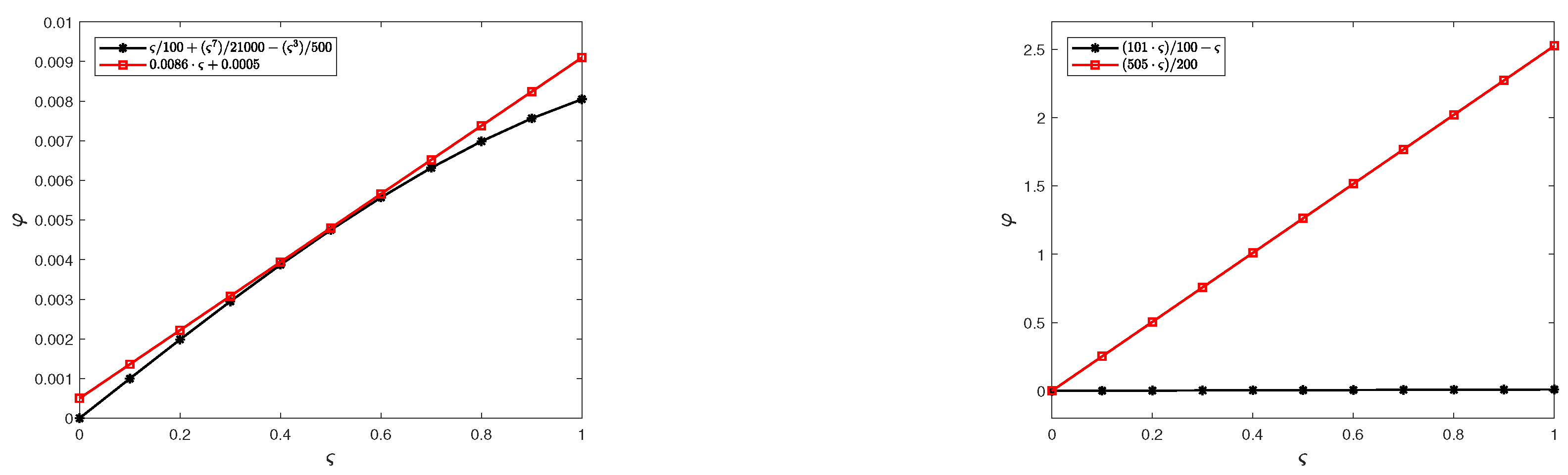
Example 1.

Firstly, we consider the integral equation

$$\begin{array}{c}\hfill \phi \left(\varsigma \right)={\displaystyle \frac{{\varsigma }^7}{210}}-{\displaystyle \frac{{\varsigma }^3}{5}}+\varsigma +{\displaystyle \frac{\phi \left({\beta }_1\left(\varsigma \right)\right)}{5}}+{\displaystyle \frac{1}{5}}{\int }_0^{\varsigma }\left((\ell -\varsigma )\phi \left({\beta }_2(\ell )\right)\right)d\ell ,\end{array}$$

(37)

where $\varsigma \in [0,1]$, $\phi :[0,1]\to R$ is a continuous function, ${\beta }_1:[0,1]\to [0,1]$ and ${\beta }_2:[0,1]\to [0,1]$ are two continuous delay functions, defined as ${\beta }_1\left(\varsigma \right)={\varsigma }^3$ and ${\beta }_2\left(\varsigma \right)={\varsigma }^5$. Also, ${\beta }_1\left(\varsigma \right)\le \varsigma$ and ${\beta }_2\left(\varsigma \right)\le \varsigma$ for all $\varsigma \in [0,1]$. Hence, all the conditions of Theorem 5 are satisfied. Now, $g:[0,1]\times \mathbb{C}\times \mathbb{C}\times \mathbb{C}\to \mathbb{C}$ given as

$$\begin{array}{c}\hfill g(\varsigma ,\phi \left(\varsigma \right),\phi \left(\alpha \left(\varsigma \right)\right),f\left(\varsigma \right))={\displaystyle \frac{{\varsigma }^7}{210}}-{\displaystyle \frac{{\varsigma }^3}{5}}+\varsigma +{\displaystyle \frac{\phi \left({\beta }_1\left(\varsigma \right)\right)}{5}}+{\displaystyle \frac{f\left(\varsigma \right)}{5}}\end{array}$$

is a continuous function fulfilling

$$\begin{array}{ccc}\hfill \left|g\right(\varsigma ,\mu \left(\varsigma \right),\mu \left({\beta }_1\left(\varsigma \right)\right),f_1\left(\varsigma \right))& -& g(\varsigma ,\upsilon \left(\varsigma \right),\upsilon \left({\beta }_1\left(\varsigma \right)\right),f_2\left(\varsigma \right))|\hfill \\ \hfill & \le & {\displaystyle \frac{1}{5}}\left(\right|\mu \left(\varsigma \right)-\upsilon \left(\varsigma \right)|+|\mu \left({\beta }_1\left(\varsigma \right)\right)-\upsilon \left({\beta }_1\left(\varsigma \right)\right)|\hfill \\ & +& |f_1\left(\varsigma \right)-f_2\left(\varsigma \right)\left|\right)\hfill \end{array}$$

(38)

for all $\varsigma \in [0,1].$ Here, the value of the $M={\displaystyle \frac{1}{5}}$, the kernel $k:[0,1]\times [0,1]\times \mathbb{C}\times \mathbb{C}\to \mathbb{C}$ defined as $\kappa (\varsigma ,\ell ,\phi (\ell ),\phi \left({\beta }_2(\ell )\right))=(\ell -\varsigma )\phi \left({\beta }_2(\ell )\right)$ is a continuous function, which satisfies the following condition

$$\begin{array}{c}\hfill |\kappa (\varsigma ,\ell ,\mu (\ell ),\mu \left({\beta }_2(\ell )\right))-\kappa (\varsigma ,\ell ,\upsilon (\ell ),\upsilon \left({\beta }_2(\ell )\right))|\le |\mu \left({\beta }_2(\ell )\right)-\mu \left({\beta }_2(\ell )\right)|,\ell \in [0,\varsigma ],\varsigma \in [0,1],\end{array}$$

(39)

here, $L=1$. Thus, taking $\eta =1$, we obtain $M(2+L(d-c\left)\right)<1$. If we choose $\phi \left(\varsigma \right)={\displaystyle \frac{101\varsigma }{100}}$, it follows

$$\begin{array}{ccc}\hfill {\displaystyle |}\phi \left(\varsigma \right)& -& g\left(\varsigma ,\phi \left(\varsigma \right),\phi \left({\beta }_1\left(\varsigma \right)\right),{\int }_0^{\varsigma }\kappa (\varsigma ,\ell ,\phi (\ell ),\phi \left({\beta }_2(\ell )\right))d\ell \right){\displaystyle |}\hfill \\ & =& |{\displaystyle \frac{\varsigma }{100}}+{\displaystyle \frac{{\varsigma }^7}{21000}}-{\displaystyle \frac{{\varsigma }^3}{500}}|\le 0.0086\varsigma +0.0005=\varphi \left(\varsigma \right).\hfill \end{array}$$

(40)

Thus, we obtain the HUR stability of the integral Equation (37) from Theorem 5. Considering the specific solution ${\phi }_0\left(\varsigma \right)=\varsigma$ for Equation (37), we have

$$\begin{array}{c}\hfill |\phi \left(\varsigma \right)-{\phi }_0\left(\varsigma \right)|=|{\displaystyle \frac{101}{100}}\varsigma -\varsigma |\le {\displaystyle \frac{1}{1-M(2+L(d-c\left)\right)}}\varphi \left(\varsigma \right)={\displaystyle \frac{5}{2}}\varphi \left(\varsigma \right).\end{array}$$

(41)

The comparison between the two functions using the inequalities (40) and (41) is shown in Figure 1.

4. Stability of Integro-Differential Equation

In this section, we will find a sufficient condition for the HU–Rassias and HU stabilities of the following integro-differential equation

$$\begin{array}{c}\hfill {\phi }^{\prime }\left(\varsigma \right)=g\left(\varsigma ,\phi \left(\varsigma \right),\phi \left({\beta }_1\left(\varsigma \right)\right),{\int }_c^{\varsigma }\kappa (\varsigma ,\ell ,\phi (\ell ),\phi \left({\beta }_2(\ell )\right))d\ell \right),\end{array}$$

(42)

where $\varsigma \in [\mathsf{c},\mathsf{d}]$. Also, we consider the space $C^1[\mathsf{c},\mathsf{d}]$ as the set of all functions that are continuously differentiable on the interval $[\mathsf{c},\mathsf{d}]$. This space is equipped with a metric known as the b-metric defined as

$$\begin{array}{c}\hfill d(\mu ,\upsilon )=\underset{\varsigma \in [\mathsf{c},\mathsf{d}]}{sup}\left\{\eta \right|\mu \left(\varsigma \right)-\upsilon \left(\varsigma \right)\left|\right\}\end{array}$$

(43)

and the space $C^1[\mathsf{c},\mathsf{d}]$ is a complete metric space in the sense of the b-metric function.

Theorem 6.

Let $g:[\mathsf{c},\mathsf{d}]\times \mathbb{C}\times \mathbb{C}\times \mathbb{C}\to \mathbb{C}$ be a continuous function which satisfies the Lipschitz condition

$$\begin{array}{ccc}\hfill \left|g\right(\varsigma ,\mu \left(\varsigma \right),\mu \left({\beta }_1\left(\varsigma \right)\right),f_1\left(\varsigma \right))& -& g(\varsigma ,\upsilon \left(\varsigma \right),\upsilon \left({\beta }_1\left(\varsigma \right)\right),f_2\left(\varsigma \right))|\hfill \\ \hfill & \le & M\left(\right|\mu \left(\varsigma \right)-\upsilon \left(\varsigma \right)|+|\mu \left({\beta }_1\left(\varsigma \right)\right)-\upsilon \left({\beta }_1\left(\varsigma \right)\right)\hfill \\ & +& |f_1\left(\varsigma \right)-f_2\left(\varsigma \right)\left|\right),\hfill \end{array}$$

(44)

where $M>0$ and $k:[\mathsf{c},\mathsf{d}]\times [\mathsf{c},\mathsf{d}]\times \mathbb{C}\times \mathbb{C}\to \mathbb{C}$ is the kernel, which also satisfies the Lipschitz condition

$$\begin{array}{cc}\hfill \left|\kappa \right(\varsigma ,\ell ,\mu (\ell ),\mu \left({\beta }_2(\ell )\right)-\kappa (\varsigma ,\ell ,\upsilon (\ell ),\upsilon \left({\beta }_2(\ell )\right)|\le L|\mu \left({\beta }_2(\ell )\right)-\upsilon \left({\beta }_1(\ell )\right)|,& L>0.\end{array}$$

(45)

If $\phi \in C^1[\mathsf{c},\mathsf{d}]$ follows

$$\begin{array}{c}\hfill |{\phi }^{\prime }\left(\varsigma \right)-g\left(\varsigma ,\phi \left(\varsigma \right),\phi \left({\beta }_1\left(\varsigma \right)\right),{\int }_c^{\varsigma }\kappa (\varsigma ,\ell ,\phi (\ell ),\phi \left({\beta }_2(\ell )\right))d\ell \right)|\le \varphi \left(\varsigma \right)\end{array}$$

(46)

and $M(2(d-c)+L{(d-c)}^2)<1$, then there exists a function ${\phi }_0\in C^1[\mathsf{c},\mathsf{d}]$ which is unique, such that

$$\begin{array}{c}\hfill {\phi }_0^{\prime }\left(\varsigma \right)=g\left(\varsigma ,{\phi }_0\left(\varsigma \right),{\phi }_0\left({\beta }_1\left(\varsigma \right)\right),{\int }_c^{\varsigma }\kappa (\varsigma ,\ell ,{\phi }_0(\ell ),{\phi }_0\left({\beta }_2(\ell )\right))d\ell \right)\end{array}$$

(47)

and

$$\begin{array}{c}\hfill |\phi \left(\varsigma \right)-{\phi }_0\left(\varsigma \right)|\le {\displaystyle \frac{\varphi \left(\varsigma \right)}{1-M(2(d-c)+L{(d-c)}^2)}}.\end{array}$$

(48)

Proof. 

If we integrate the Equation (42), we obtain

$$\begin{array}{c}\hfill \phi \left(\varsigma \right)=a+{\int }_c^{\varsigma }g\left(z,\phi \left(z\right),\phi \left({\beta }_1\left(z\right)\right),{\int }_c^{z}k(z,\ell ,\phi (\ell ),\phi \left({\beta }_2(\ell )\right))d\ell \right)dz.\end{array}$$

(49)

We define the operator $T:C[\mathsf{c},\mathsf{d}]\to C[\mathsf{c},\mathsf{d}]$, such that

$$\begin{array}{c}\hfill T\left(\mu \right)\left(\varsigma \right)=a+{\int }_c^{\varsigma }g\left(z,\mu \left(z\right),\mu \left({\beta }_1\left(z\right)\right),{\int }_c^{z}k(z,\ell ,\mu (\ell ),\mu \left({\beta }_2(\ell )\right))d\ell \right)dz,\end{array}$$

(50)

for all $\varsigma \in [\mathsf{c},\mathsf{d}]$ and $\mu \in C^1[\mathsf{c},\mathsf{d}]$. Now, we will prove that for any continuous function $\mu$, $T\mu$ is also continuous.

$$\begin{array}{ccc}\hfill |\left(T\mu \right)\left(\varsigma \right)-\left(T\mu \right)\left({\varsigma }_0\right)|& =& |{\int }_c^{\varsigma }g\left(z,\mu \left(z\right),\mu \left({\beta }_1\left(z\right)\right),{\int }_c^{z}k(z,\ell ,\mu (\ell ),\mu \left({\beta }_2(\ell )\right))d\ell \right)dz\hfill \\ & -& {\int }_c^{{\varsigma }_0}g\left(z,\mu \left(z\right),\mu \left({\beta }_1\left(z\right)\right),{\int }_c^{z}k(z,\ell ,\mu (\ell ),\mu \left({\beta }_2(\ell )\right))d\ell \right)dz|\hfill \\ & =& \left|{\int }_{\varsigma }^{{\varsigma }_0}g\left(z,\mu \left(z\right),\mu \left({\beta }_1\left(z\right)\right),{\int }_c^{z}k(z,\ell ,\mu (\ell ),\mu \left({\beta }_2(\ell )\right))d\ell \right)dz\right|\to 0,\hfill \end{array}$$

when $\varsigma \to {\varsigma }_0$. Next, we will prove T is the strictly contractive operator with respect to the metric defined in (1). Now, for all $\mu ,\upsilon \in C^1[\mathsf{c},\mathsf{d}]$,

$$\begin{array}{ccc}\hfill d_b(T\mu ,T\upsilon )& =& \underset{\varsigma \in [\mathsf{c},\mathsf{d}]}{sup}\left\{\eta \right|\left(T\mu \right)\left(\varsigma \right)-\left(T\upsilon \right)\left(\varsigma \right)\left|\right\}\hfill \\ & =& \eta \underset{\varsigma \in [\mathsf{c},\mathsf{d}]}{sup}|{\int }_c^{\varsigma }g\left(z,\mu \left(z\right),\mu \left({\beta }_1\left(z\right)\right),{\int }_c^{z}k(z,\ell ,\mu (\ell ),\mu \left({\beta }_2(\ell )\right))d\ell \right)dz\hfill \\ & -& {\int }_c^{\varsigma }g\left(z,\upsilon \left(z\right),\upsilon \left({\beta }_1\left(z\right)\right),{\int }_c^{z}k(s,\ell ,\upsilon (\ell ),\upsilon \left({\beta }_2(\ell )\right))d\ell \right)dz|\hfill \\ & \le & \eta M\underset{\varsigma \in [\mathsf{c},\mathsf{d}]}{sup}{\int }_c^{\varsigma }|\mu \left(z\right)-\upsilon \left(z\right)|dz\hfill \\ & +& \eta M\underset{\varsigma \in [\mathsf{c},\mathsf{d}]}{sup}{\int }_c^{\varsigma }|\mu \left({\beta }_1\left(z\right)\right)-\upsilon \left({\beta }_1\left(z\right)\right)|dz\hfill \\ & +& \eta M\underset{\varsigma \in [\mathsf{c},\mathsf{d}]}{sup}{\int }_c^{\varsigma }{\int }_c^z|k(z,\ell ,\mu (\ell ),\mu \left({\beta }_2(\ell )\right))\hfill \\ & -& k(z,\ell ,\upsilon (\ell ),\upsilon \left({\beta }_2(\ell )\right))|d\ell dz\hfill \\ & \le & \eta M\underset{\varsigma \in [\mathsf{c},\mathsf{d}]}{sup}{\int }_c^{\varsigma }\left\{\right|\mu \left(z\right)-\upsilon \left(z\right)|dz\hfill \\ & +& \eta M\underset{\varsigma \in [\mathsf{c},\mathsf{d}]}{sup}{\int }_c^{\varsigma }|\mu \left({\beta }_1\left(z\right)\right)-\upsilon \left({\beta }_1\left(z\right)\right)|dz\hfill \\ & +& \eta M\underset{\varsigma \in [\mathsf{c},\mathsf{d}]}{sup}{\int }_c^{\varsigma }{\int }_c^z|k(z,\ell ,\mu (\ell ),\mu \left({\beta }_2(\ell )\right))-k(z,\ell ,\upsilon (\ell ),\upsilon \left({\beta }_2(\ell )\right))|d\ell dz\hfill \\ & \le & \eta M\underset{\varsigma \in [\mathsf{c},\mathsf{d}]}{sup}{\int }_c^{\varsigma }\left\{\right|\mu \left(z\right)-\upsilon \left(z\right)|dz\hfill \\ & +& \eta M\underset{\varsigma \in [\mathsf{c},\mathsf{d}]}{sup}{\int }_c^{\varsigma }|\mu \left({\beta }_1(\ell )\right)-\upsilon \left({\beta }_1(\ell )\right)|d\ell \hfill \\ & +& L\eta M\underset{\varsigma \in [\mathsf{c},\mathsf{d}]}{sup}{\int }_c^{\varsigma }{\int }_c^z|\mu \left({\beta }_2(\ell )\right)-\upsilon \left({\beta }_2(\ell )\right)|d\ell dz\hfill \\ & \le & 2\eta M\underset{\varsigma \in [\mathsf{c},\mathsf{d}]}{sup}{\int }_c^{\varsigma }|\mu \left(z\right)-\upsilon \left(z\right)|dz\hfill \\ & +& \eta ML\underset{\varsigma \in [\mathsf{c},\mathsf{d}]}{sup}{\int }_c^{\varsigma }{\int }_c^z|\mu \left({\beta }_2(\ell )\right)-\upsilon \left({\beta }_2(\ell )\right)|d\ell dz\hfill \\ & \le & 2M\eta \underset{z\in [\mathsf{c},\mathsf{d}]}{sup}|\mu \left(z\right)-\upsilon \left(z\right)|\underset{\varsigma \in [\mathsf{c},\mathsf{d}]}{sup}{\int }_c^{\varsigma }dz\hfill \\ & +& L\eta M\underset{\ell \in [\mathsf{c},\mathsf{d}]}{sup}\left\{\right|\mu (\ell )-\upsilon (\ell )\left|\right\}\underset{\varsigma \in [\mathsf{c},\mathsf{d}]}{sup}{\int }_c^{\varsigma }{\int }_c^{z}d\ell dz\hfill \\ & \le & M\{2d_b(\mu ,\upsilon )(d-c)+L\eta {(d-c)}^2{d}_b(\mu ,\upsilon )\}\hfill \\ & =& M(2(d-c)+L{(d-c)}^2)d_b(\mu ,\upsilon ).\hfill \end{array}$$

Hence, using the assumption that $M(2(d-c)+L{(d-c)}^2)<1$, we conclude that T is a strictly contractive operator. Hence, we can utilize the previously established the Banach Fixed-Point Theorem [20], which assures the HU stability for the integral-differential equation. Moreover, by applying the Banach Fixed-Point Theorem [18,20] once more and using the inequality (31) and the definition of $d_b$-metric, it follows that

$$\begin{array}{c}\hfill \underset{\varsigma \in [\mathsf{c},\mathsf{d}]}{sup}\eta |\phi \left(\varsigma \right)-{\phi }_0\left(\varsigma \right)|\le {\displaystyle \frac{\eta \varphi \left(\varsigma \right)}{1-M(2(d-c)+L{(d-c)}^2)}}.\end{array}$$

(51)

Hence, it implies that

$$\begin{array}{c}\hfill |\phi \left(\varsigma \right)-{\phi }_0\left(\varsigma \right)|\le {\displaystyle \frac{\varphi \left(\varsigma \right)}{1-M(2(d-c)+L{(d-c)}^2)}}.\end{array}$$

(52)

□

This implies that, under the given conditions, the given integro-differential equation possesses Hyer–Ulam–Rassias stability.

Theorem 7.

Let $g:[\mathsf{c},\mathsf{d}]\times \mathbb{C}\times \mathbb{C}\times \mathbb{C}\to \mathbb{C}$ be a continuous function that satisfies the Lipschitz condition

$${\displaystyle \begin{array}{cc}\hfill \left|g\right(\varsigma ,\mu \left(\varsigma \right),\mu \left({\beta }_1\left(\varsigma \right)\right),f_1\left(\varsigma \right))& -g(\varsigma ,\upsilon \left(\varsigma \right),\upsilon \left({\beta }_1\left(\varsigma \right)\right),f_2\left(\varsigma \right))|\hfill \\ \hfill & \le M\left(\right|\mu \left(\varsigma \right)-\upsilon \left(\varsigma \right)|+|\mu \left({\beta }_1\left(\varsigma \right)\right)-\upsilon \left({\beta }_1\left(\varsigma \right)\right)+|f_1\left(\varsigma \right)-f_2\left(\varsigma \right)|),\hfill \end{array}}$$

where $M>0$ and $k:[\mathsf{c},\mathsf{d}]\times [\mathsf{c},\mathsf{d}]\times \mathbb{C}\times \mathbb{C}\to \mathbb{C}$ is the kernel, which also satisfies the Lipschitz condition

$$\begin{array}{cc}\hfill \left|\kappa \right(\varsigma ,\ell ,\mu (\ell ),\mu \left({\beta }_2(\ell )\right)-\kappa (\varsigma ,\ell ,\upsilon (\ell ),\upsilon \left({\beta }_2(\ell )\right)|\le L|\mu \left({\beta }_2(\ell )\right)-\upsilon \left({\beta }_1(\ell )\right)|,& L>0.\end{array}$$

(53)

If $\phi \in C^1[\mathsf{c},\mathsf{d}]$ follows

$$\begin{array}{c}\hfill |{\phi }^{\prime }\left(\varsigma \right)-g\left(\varsigma ,\phi \left(\varsigma \right),\phi \left({\beta }_1\left(\varsigma \right)\right),{\int }_c^{\varsigma }\kappa (\varsigma ,\ell ,\phi (\ell ),\phi \left({\beta }_2(\ell )\right))d\ell \right)|\le \lambda \end{array}$$

(54)

and $M(2(d-c)+L{(d-c)}^2)<1$, then there exists a function ${\phi }_0\in C^1[\mathsf{c},\mathsf{d}]$ which is unique, such that

$$\begin{array}{c}\hfill {\phi }_0^{\prime }\left(\varsigma \right)=g\left(\varsigma ,{\phi }_0\left(\varsigma \right),{\phi }_0\left({\beta }_1\left(\varsigma \right)\right),{\int }_c^{\varsigma }\kappa (\varsigma ,\ell ,{\phi }_0(\ell ),{\phi }_0\left({\beta }_2(\ell )\right))d\ell \right)\end{array}$$

(55)

and

$$\begin{array}{c}\hfill |\phi \left(\varsigma \right)-{\phi }_0\left(\varsigma \right)|\le {\displaystyle \frac{\lambda }{1-M(2(d-c)+L{(d-c)}^2)}}.\end{array}$$

(56)

Proof. 

Consider the operator $T:C[\mathsf{c},\mathsf{d}]\to C[\mathsf{c},\mathsf{d}]$, such that

$$\begin{array}{c}\hfill T\left(\mu \right)\left(\varsigma \right)=a+{\int }_c^{\varsigma }g\left(z,\mu \left(z\right),\mu \left({\beta }_1\left(z\right)\right),{\int }_c^{z}k(z,\ell ,\mu (\ell ),\mu \left({\beta }_2(\ell )\right))d\ell \right)dz,\end{array}$$

(57)

for all $\varsigma \in [\mathsf{c},\mathsf{d}]$ and $\mu \in C[\mathsf{c},\mathsf{d}]$. Now, by following the same procedure as that used in the proof of Theorem 6, we can conclude that T is strictly contractive with respect to the metric defined in (1) since $M(2(d-c)+L{(d-c)}^2)<1$. Hence, we can utilize the previously established the Banach Fixed-Point Theorem [20], which assures the HU–Rassias stability for the integral equation. Moreover, by applying the Banach Fixed-Point Theorem [18,20] once more and using the inequality (54) and definition of $d_b$-metric, it follows that

$$\begin{array}{c}\hfill |\phi \left(\varsigma \right)-{\phi }_0\left(\varsigma \right)|\le {\displaystyle \frac{\lambda }{1-M(2(d-c)+L{(d-c)}^2)}}.\end{array}$$

(58)

□

This implies that, under the given conditions, the given integro-differential equation possesses Hyer–Ulam stability.

Example 2.

Firstly, we consider the integral equation

$$\begin{array}{c}\hfill \phi \left(\varsigma \right)={\displaystyle \frac{s{e}^{\frac{\varsigma }{2}}}{6}}+{\displaystyle \frac{e^{\frac{\varsigma }{2}}}{3}}+{\displaystyle \frac{2\phi \left({\beta }_1\left(\varsigma \right)\right)}{3}}-{\displaystyle \frac{e^{\frac{\varsigma }{2}}}{12}}{\int }_0^{\varsigma }\left((\ell -\varsigma )\phi \left({\beta }_2(\ell )\right)\right)d\ell ,\end{array}$$

(59)

where $\varsigma \in [0,1]$, $\phi :[0,1]\to R$ is a continuous function, ${\beta }_1:[0,1]\to [0,1]$ and ${\beta }_2:[0,1]\to [0,{\displaystyle \frac{1}{2}}]$ are two continuous delay functions, defined as ${\beta }_1\left(\varsigma \right)=\varsigma$ and ${\beta }_2\left(\varsigma \right)={\displaystyle \frac{\varsigma }{2}}$. Also, ${\beta }_1\left(\varsigma \right)\le \varsigma$ and ${\beta }_2\left(\varsigma \right)\le \varsigma$ for all $\varsigma \in [0,1]$. Hence, all the conditions of Theorem 6 are satisfied. Now, $g:[0,1]\times \mathbb{C}\times \mathbb{C}\times \mathbb{C}\to \mathbb{C}$ defined by

$$\begin{array}{c}\hfill g(\varsigma ,\phi \left(\varsigma \right),\phi \left(\alpha \left(\varsigma \right)\right),f\left(\varsigma \right))={\displaystyle \frac{\varsigma e^{\frac{\varsigma }{2}}}{6}}+{\displaystyle \frac{e^{\frac{\varsigma }{2}}}{3}}+{\displaystyle \frac{2\phi \left({\beta }_1\left(\varsigma \right)\right)}{3}}-{\displaystyle \frac{e^{\frac{\varsigma }{2}}}{12}}g\left(\varsigma \right)\end{array}$$

is a continuous function fulfilling

$$\begin{array}{ccc}\hfill \left|g\right(\varsigma ,\mu \left(\varsigma \right),\mu \left({\beta }_1\left(\varsigma \right)\right),f_1\left(\varsigma \right))& -& g(\varsigma ,\upsilon \left(\varsigma \right),\upsilon \left({\beta }_1\left(\varsigma \right)\right),f_2\left(\varsigma \right))|\hfill \\ & \le & {\displaystyle \frac{e^{\frac{1}{2}}}{12}}\left(\right|\mu \left(\varsigma \right)-\upsilon \left(\varsigma \right)|+|\mu \left({\beta }_1\left(\varsigma \right)\right)-\upsilon \left({\beta }_1\left(\varsigma \right)\right)|\hfill \\ & +& |f_1\left(\varsigma \right)-f_2\left(\varsigma \right)\left|\right)\hfill \end{array}$$

(60)

for all $\varsigma \in [0,1].$ Here, the value of $M={\displaystyle \frac{e^{\frac{1}{2}}}{12}}$, the kernel $k:[0,1]\times [0,1]\times \mathbb{C}\times \mathbb{C}\to \mathbb{C}$ defined by $\kappa (\varsigma ,\ell ,\phi (\ell ),\phi \left({\beta }_2\left(\varsigma \right)\right))=(\ell -\varsigma )\phi \left({\beta }_2(\ell )\right)$ is a continuous function, which satisfies the following condition

$$\begin{array}{c}\hfill |k(\varsigma ,\mu (\ell ),\mu \left({\beta }_2(\ell )\right))-\kappa (\varsigma ,\ell ,\upsilon (\ell ),\upsilon \left({\beta }_2(\ell )\right))|\le |\mu \left({\beta }_2(\ell )\right)-\mu \left({\beta }_2(\ell )\right)|,\ell \in [0,\varsigma ],\varsigma \in [0,1],\end{array}$$

(61)

here, $L=1$. Thus, taking $\eta =1$, we obtain $M(2(d-c)+L{(d-c)}^2)={\displaystyle \frac{3\sqrt{e}}{12}}<1$. If we take $\phi \left(\varsigma \right)={\displaystyle \frac{100e^{\varsigma }}{99}}$, then we have

$$\begin{array}{ccc}\hfill {\displaystyle |}{\phi }^{\prime }\left(\varsigma \right)& -& g\left(\varsigma ,\phi \left(\varsigma \right),\phi \left({\beta }_1\left(\varsigma \right)\right),{\int }_0^{\varsigma }\kappa (\varsigma ,\ell ,\phi (\ell ),\phi \left({\beta }_2(\ell )\right))d\ell \right)|\hfill \\ & =& |{\displaystyle \frac{\varsigma e^{\frac{\varsigma }{2}}}{594}}+{\displaystyle \frac{e^{\frac{\varsigma }{2}}}{297}}|\le (0.002\varsigma +0.004)e^{{\displaystyle \frac{\varsigma }{2}}}=\varphi \left(\varsigma \right).\hfill \end{array}$$

(62)

Thus, we obtain the HUR stability of the integral Equation (59) from Theorem 6. Considering the specific solution ${\phi }_0\left(\varsigma \right)=e^{\varsigma }$ for Equation (59), we have

$$\begin{array}{c}\hfill |\phi \left(\varsigma \right)-{\phi }_0\left(\varsigma \right)|={\displaystyle |}{\displaystyle \frac{100}{99}}{e}^{\varsigma }-e^{\varsigma }|\le {\displaystyle \frac{1}{1-M(2(d-c)+L{(d-c)}^2)}}\varphi \left(\varsigma \right)={\displaystyle \frac{4}{4-\sqrt{e}}}\varphi \left(\varsigma \right).\end{array}$$

(63)

The comparison between the two functions using the inequalities (62) and (63) is shown in Figure 2.

5. Advantages of Employing the B-Metric

The stability analysis in the b-metric spaces presents several advantages compared with standard metric spaces.

• B-metric spaces broaden the definition of metric spaces by allowing for a more adaptable distance function, hence enhancing stability analysis in contexts where standard metric spaces may be excessively restrictive. This comprehensive technique helps with the analysis of stability in situations that do not strictly adhere to metric space criteria, hence expanding the relevance of stability results.
• B-metric spaces provide greater flexibility in dealing with functional equations. This can lead to new stability results or more refined conditions that may not be achievable in standard metric spaces.
• The stability results obtained in b-metric spaces essentially encompass those in metric spaces, establishing an integrated framework applicable to both standard and generalized contexts. This increases the versatility of the results and broadens their applicability to a wider range of problems.
• B-metrics can be utilized to define flexible distance measures for clustering algorithms, enabling better handling of noisy or high-dimensional data. Also, this metric provide a framework for analyzing the convergence of iterative optimization methods commonly used in training machine learning models.
• Numerous practical applications, particularly in areas such as functional analysis, differential equations, and dynamic systems, encompass structures that dynamically coincide with b-metric spaces. Consequently, stability findings in b-metric spaces are frequently more relevant to practical issues than those limited to metric spaces.

In conclusion, stability analysis in b-metric spaces offers a more adaptable, comprehensive, and practical framework, allowing researchers to deal with more kinds of stability problems and to integrate the findings across various kinds of spaces.

6. Conclusions

In this work, we analyzed the stability of nonlinear Volterra and Fredholm integral equations, as well as nonlinear integro-differential equations, using fixed-point methods in b-metric spaces. The results show that the conditions for Hyers–Ulam–Rassias and Hyers–Ulam stability are more general than those in standard metric spaces due to the extended nature of b-metric spaces. Our findings reveal that stability in b-metric spaces accommodate cases that traditional metric spaces cannot, offering a more versatile theoretical framework. The practical examples provided underscore the applicability of these results, suggesting potential extensions to other types of functional equations and systems, thereby enhancing the broader understanding of stability theory in nonlinear analysis.

We propose that researchers investigate the semi-Ulam–Hyers stability of the functional equations presented in this study within the framework of other generalized metric spaces. Exploring this stability across diverse mathematical structures could provide new insights and expand the applicability of the results obtained herein.

References

1. Castro, L.P.; Ramos, A. HU-Rassias stability for a class of nonlinear Volterra integral equations. Banach J. Math. Anal. 2009, 3, 36–43. [Google Scholar] [CrossRef]
2. Castro, L.P.; Simoes, A.M. Different types of HU-Rassias stabilities for a class of integro-differential equations. Filomat 2017, 31, 5379–5390. [Google Scholar] [CrossRef]
3. Zhang, D.; Liu, Q.; Rassias, J.M.; Li, Y. The Stability of Functional Equations with a New Direct Method. Mathematics 2022, 10, 1188. [Google Scholar] [CrossRef]
4. Jakhar, J.; Sharma, S.; Jakhar, J.; Yousif, M.A.; Mohammed, P.O.; Lupas, A.A.; Chorfi, N. Orthogonal Stability and Solution of a Three-Variable Functional Equation in Extended Banach Spaces. Mathematics 2024, 18, 2868. [Google Scholar] [CrossRef]
5. Ahmad Aloqaily, P.; Agilan, K.; Julietraja, S.; Annadurai, S.; Mlaiki, N. A novel stability analysis of functional equations in neutrosophic normed spaces. Bound. Value Probl. 2024, 47, 2024. [Google Scholar] [CrossRef]
6. Burton, T.A.; Zhang, B. Fixed points and stability of an integral equation: Nonuniqueness. Appl. Math. Lett. 2004, 7, 839–846. [Google Scholar] [CrossRef]
7. Grossman, S.I. Existence and stability of a class of nonlinear Volterra integral equations. Trans. Am. Math. Soc. 1970, 2, 541–556. [Google Scholar] [CrossRef]
8. Czerwik, S. Contraction mappings in b-metric spaces. Acta. Math. Univ. Ostrav. 1993, 1, 5–11. [Google Scholar]
9. Heinonen, J. Lectures on Analysis on Metric Spaces; Universitext; Springer: Berlin/Heidelberg, Germany, 2001. [Google Scholar]
10. Sevgin, S.; Sevli, H. Stability of a nonlinear Volterra integro-differential equation via a fixed point approach. J. Nonlinear Sci. Appl. 2016, 19, 200–207. [Google Scholar] [CrossRef]
11. Yousif, M.A.; Guirao, J.L.G.; Mohammed, P.O.; Chorfi, N.; Baleanu, D. A computational study of time-fractional gas dynamics models by means of conformable finite difference method. AIMS Math. 2024, 9, 19843–19858. [Google Scholar] [CrossRef]
12. Yousif, M.A.; Agarwal, R.P.; Mohammed, P.O.; Lupas, A.A.; Jan, R.; Chorfi, N. Advanced Methods for Conformable Time-Fractional Differential Equations: Logarithmic Non-Polynomial Splines. Axioms 2024, 13, 551. [Google Scholar] [CrossRef]
13. Yousif, M.A.; Hamasalh, F.K. The fractional non-polynomial spline method: Precision and modeling improvements. Math. Comput. Simul. 2024, 218, 512–525. [Google Scholar] [CrossRef]
14. Ulam, S.M. A Collection of Mathematical Problems. In Interscience Tracts in Pure and Applied Mathematics; Wiley Interscience: New York, NY, USA, 1960. [Google Scholar]
15. Hyers, D.H. On the stability of linear functional equation. Proc. Natl. Acad. Sci. USA 1941, 27, 222–224. [Google Scholar] [CrossRef] [PubMed]
16. Rassias, T.M. On the stability of linear mapping in Banach spaces. Proc. Amer. Math. Soc. 1978, 72, 297–300. [Google Scholar] [CrossRef]
17. Czerwik, S. Nonlinear set-valued contraction mappings in b-metric spaces. Atti Del Semin. Mat. Fis. Univ. Modena 1998, 46, 263–276. [Google Scholar]
18. Brzdek, J. Comments on fixed point results in classes of function with values in a b–metric space. Rev. Real Acad. Cienc. Exactas FíSicas Nat. Ser. MatemáTicas 2022, 116, 35. [Google Scholar] [CrossRef]
19. Berinde, V.; Păcurar, M. The early developments in fixed point theory on b-metric spaces. Carpathian J. Math. 2022, 3, 523–538. [Google Scholar] [CrossRef]
20. Diaz, J.B.; Margolis, B. A fixed point theorem of the alternative, for contractions on a generalized complete metric space. Bull. Amer. Math. Soc. 1968, 74, 305–309. [Google Scholar] [CrossRef]
Figure 1. The figure on the (left) represents the comparison between the two functions using the inequality (40) and the figure on the (right) represents a comparison between the two functions using the inequality (41).
Symmetry 17 00168 g001
Figure 2. The figure on the (left) represents a comparison between the two functions using the inequality (62) and the figure on the (right) represents the comparison between the two functions using the inequality (63).
Symmetry 17 00168 g002
Disclaimer/Publisher’s Note: The statements, opinions and data contained in all publications are solely those of the individual author(s) and contributor(s) and not of MDPI and/or the editor(s). MDPI and/or the editor(s) disclaim responsibility for any injury to people or property resulting from any ideas, methods, instructions or products referred to in the content.