Bratteli Diagrams, Hopf–Galois Extensions and Calculi

Abstract

Hopf–Galois extensions extend the idea of principal bundles to noncommutative geometry, using Hopf algebras as symmetries. We show that the matrix embeddings in Bratteli diagrams are iterated direct sums of Hopf–Galois extensions (quantum principal bundles) for certain finite abelian groups. The corresponding strong universal connections are computed. We show that $M_n\left(\mathbb{C}\right)$ is a trivial quantum principle bundle for the Hopf algebra $\mathbb{C}[{\mathbb{Z}}_n\times {\mathbb{Z}}_n]$. We conclude with an application relating calculi on groups to calculi on matrices.

1. Introduction

The idea of using a Hopf algebra in place of a symmetry group to give a definition of a principal bundle in noncommutative geometry was given in [1]. (Independently in [2,3] this was described in terms of differential calculi.) Because of the connection between classical Galois theory and this definition of principal bundles, they were called Hopf–Galois extensions (see [4,5,6]). These extensions generalise the classical idea by taking complex functions on the base space of the principal fibration to be included in functions on the total space as functions constant on each fibre, and is described in more detail in Section 2.

In 1972 Ola Bratteli introduced graphs for describing a certain class of $C^{*}$-algebras (the approximately finite-dimensional or AF $C^{*}$-algebras) in terms of the limits of direct sums of matrices [7]. This is a graph split into levels, and an example of one level in a Bratteli digram is

(1)

which represents the map

$$\begin{array}{c}\hfill \left(a\right)\oplus \left(\begin{array}{cc}b& c\\ d& e\end{array}\right)\mapsto \left(a\right)\oplus \left(\begin{array}{cccc}a& 0& 0& 0\\ 0& a& 0& 0\\ 0& 0& b& c\\ 0& 0& d& e\end{array}\right).\end{array}$$

Here, $M_n\left(\mathbb{C}\right)$ represents n-by-n matrices with complex number entries.

In Section 3, we will show that the inclusions of algebras given by such diagrams do not necessarily give Hopf–Galois extensions. However, in this paper, we show that we can split each level on the diagram into a composition of stages, each of which is a direct sum of Hopf–Galois extensions. Taking the direct sum to be the same as the disjoint union of topological spaces, we simply allow different groups in principal bundles over different components. For example, we rewrite (1) as a composition of three stages:

(2)

and we refer to these as (from right to left) Case 1, Case 2 and Case 3. To be more explicit, the cases are described as follows: Case 1: There are not multiple lines, and every node on the left has a single line coming from it. Case 3: There are not multiple lines, and every node on the right has a single line going to it. Case 2: Each node on the right or left is connected to exactly one node. The line can be multiple. In each of these cases, we shall exhibit a strong universal connection map.

The idea of a trivial quantum principle bundle was described in [8]. In Section 7, we show that $M_n\left(\mathbb{C}\right)$ is a trivial quantum principle bundle for the Hopf algebra $\mathbb{C}[{\mathbb{Z}}_n\times {\mathbb{Z}}_n]$. Note that in [9], it was shown that $M_n\left(\mathbb{C}\right)$ was an algebra factorisation of two copies of $\mathbb{C}\left[{\mathbb{Z}}_n\right]$ satisfying a Galois condition. We give an application relating differential calculi on $M_n\left(\mathbb{C}\right)$ to differential calculi on $\mathbb{C}[{\mathbb{Z}}_n\times {\mathbb{Z}}_n]$. Then, we give our concluding remarks and present possible applications.

2. Preliminaries

For our purposes, it is sufficient to consider Hopf algebras of the form $H=\mathbb{C}\left[G\right]$ and the complex-valued functions on a finite group G. Then, H has the basis ${\delta }_g$, the function of which is 1 at $g\in G$ and zero elsewhere. The Hopf algebra operations are

$$\begin{array}{cc}\hfill {\delta }_x{\delta }_y& =\left\{\begin{array}{cc}{\delta }_x\hfill & \mathrm{if}x=y\hfill \\ 0\hfill & \mathrm{if}x\ne y\hfill \end{array}\right.\mathrm{and}\Delta {\delta }_g=\sum _{x,y\in G:xy=g}{\delta }_x\otimes {\delta }_y,\hfill \\ \hfill 1& =\sum _{x\in G}{\delta }_x,ϵ\left({\delta }_x\right)={\delta }_{x,e},S\left({\delta }_x\right)={\delta }_{x^{-1}}.\hfill \end{array}$$

We write the coproduct of H as $\Delta \left(h\right)=h_{\left(1\right)}\otimes h_{\left(2\right)}$ using the Sweedler notation.

To define a Hopf–Galois extension, we begin by supposing that P is a unital algebra and that H is a Hopf algebra over $\mathbb{C}$.

Definition 1.

For an algebra P and a Hopf algebra H, we say that a right coaction ${\Delta }_R:P\to P\otimes H$ makes P into a right H-comodule algebra if ${\Delta }_R$ is an algebra map, i.e., for $p, q\in P$

$$\begin{array}{c}\hfill {\left(pq\right)}_{\left[0\right]}\otimes {\left(pq\right)}_{\left[1\right]}=p_{\left[0\right]}{q}_{\left[0\right]}\otimes p_{\left[1\right]}{q}_{\left[1\right]},{\Delta }_R\left(1\right)=1\otimes 1,\end{array}$$

(3)

where we write the coaction as ${\Delta }_R=p_{\left[0\right]}\otimes p_{\left[1\right]}$.

This means that the invariant $A=P^{\mathrm{coH}}=\{p\in P:{\Delta }_R\left(p\right)=p\otimes 1\}$ is a subalgebra of P.

Example 1.

Suppose that K is a subgroup of the finite group G. Then, there is a right coaction of $H=\mathbb{C}\left[K\right]$ on $P=\mathbb{C}\left[G\right]$ given by

$${\Delta }_R\left({\delta }_g\right)=\sum _{k\in K}{\delta }_{kg{k}^{-1}}\otimes {\delta }_k.$$

To check that this is a right coaction, we calculate

$$\begin{array}{cc}\hfill (\mathrm{id}\otimes \Delta ){\Delta }_R\left({\delta }_g\right)& =\sum _{k\in K}{\delta }_{kg{k}^{-1}}\otimes \Delta {\delta }_k=\sum _{k,x,y\in K:xy=k}{\delta }_{kg{k}^{-1}}\otimes {\delta }_x\otimes {\delta }_y,\hfill \\ \hfill ({\Delta }_R\otimes \mathrm{id}){\Delta }_R\left({\delta }_g\right)& =\sum _{y\in K}{\Delta }_R\left({\delta }_{yg{y}^{-1}}\right)\otimes {\delta }_y=\sum _{x,y\in K:xy=k}{\delta }_{xyg{y}^{-1}{x}^{-1}}\otimes {\delta }_x\otimes {\delta }_y.\hfill \end{array}$$

These are the same, as required. Also $P=\mathbb{C}\left[G\right]$ is a right H-comodule algebra, and we check the required multiplicative property.

$$\begin{array}{cc}\hfill {\Delta }_R\left({\delta }_g\right).{\Delta }_R\left({\delta }_h\right)& =\sum _{x,y\in K}({\delta }_{xg{x}^{-1}}\otimes {\delta }_x).({\delta }_{yh{y}^{-1}}\otimes {\delta }_y)\hfill \\ \hfill & =\sum _{x,y\in K}{\delta }_{xg{x}^{-1}}\otimes {\delta }_x{\delta }_{x,y}{\delta }_{xg{x}^{-1},yh{y}^{-1}},\hfill \\ \hfill {\Delta }_R\left({\delta }_g{\delta }_h\right)& ={\Delta }_R\left({\delta }_g\right){\delta }_{g,h}=\sum _{x\in K}{\delta }_{xg{x}^{-1}}\otimes {\delta }_x{\delta }_{g,h},\hfill \end{array}$$

which are the same, as required. Finally, the invariants for the coaction are spanned by those ${\delta }_g$ obeying

$${\Delta }_R\left({\delta }_g\right)=\sum _{k\in K}{\delta }_{kg{k}^{-1}}\otimes {\delta }_k={\delta }_g\otimes 1=\sum _{k\in K}{\delta }_g\otimes {\delta }_k,$$

and thus consist of the functions on the subset of G whose elements commute with all elements of K.

Definition 2.

Let P be a right H-comodule algebra. P is a Hopf–Galois extension of $A=P^{\mathrm{coH}}$ if the canonical map $\mathrm{can}:P{\otimes }_{A}P\to P\otimes H$ is a bijection, where

$$\begin{array}{c}\hfill \mathrm{can}(p\otimes q)=p{q}_{\left[0\right]}\otimes q_{\left[1\right]}.\end{array}$$

(4)

The idea of a Hopf–Galois extension can also be described as a quantum principle bundle in the case of universal differential calculi ([10], Chapter 5). We shall return to this later and present an application to differential calculi on the matrices. If P is a Hopf–Galois extension, then there are elements of $P{\otimes }_{A}P$ mapping to $1\otimes h$ for all $h\in H$. For many practical purposes, we seek an element $h^{\left(1\right)}\otimes h^{\left(2\right)}\in P\otimes P$ (not ${\otimes }_A$) mapping to $1\otimes h$ under the canonical map. This is no longer unique, but we ask whether there is a function ${\omega }^{♯}:H\to P\otimes P$ given by ${\omega }^{♯}\left(h\right)=h^{\left(1\right)}\otimes h^{\left(2\right)}$ such that ${\omega }^{♯}\left(1\right)=1\otimes 1$ and

$$\begin{array}{cc}\hfill h^{\left(1\right)}\otimes {h^{\left(2\right)}}_{\left[0\right]}\otimes {h^{\left(2\right)}}_{\left[1\right]}& ={h_{\left(1\right)}}^{\left(1\right)}\otimes {h_{\left(1\right)}}^{\left(2\right)}\otimes h_{\left(2\right)},\hfill \\ \hfill {h^{\left(1\right)}}_{\left[0\right]}\otimes {h^{\left(1\right)}}_{\left[1\right]}\otimes h^{\left(2\right)}& ={h_{\left(2\right)}}^{\left(1\right)}\otimes S{h}_{\left(1\right)}\otimes {h_{\left(2\right)}}^{\left(2\right)}.\hfill \end{array}$$

(5)

In this case, we say that ${\omega }^{♯}$ is a strong universal connection (this name was given in [11]). In [12], it was shown that if H has a normalised integral, then ${\omega }^{♯}$ always exists, using the next result, for which we provide a framework of the proof, as we shall require it later.

Theorem 1.

Suppose that H has a normalised left-integral ∫ and bijective antipode, and that P is a right H-comodule algebra with the canonical map surjective. Then, $(P,H,{\Delta }_R)$ is a universal quantum principal bundle and admits a strong connection. To show this, begin with a linear map $h\mapsto h^{\left(1\right)}\otimes h^{\left(2\right)}\in P\otimes P$ so that $1\mapsto 1\otimes 1$ and $\mathrm{can}(h^{\left(1\right)}\otimes h^{\left(2\right)})=1\otimes h\in P\otimes H$, but not necessarily satisfying (5). Now, define $b:H\otimes H\to \mathbb{C}$ using $b(h,g)=\int \left(hSg\right)$, and then $a_R:P\otimes H\to P$ and $a_L:H\otimes P\to P$ using $a_R(p\otimes h)=p_{\left[0\right]}b(p_{\left[1\right]},h)$ and $a_L(h\otimes p)=b(h,S^{-1}{p}_{\left[1\right]})p_{\left[0\right]}$. Then, we have a strong universal connection:

$$\begin{array}{c}\hfill {\omega }^{♯}\left(h\right)=a_L(h_{\left(1\right)}\otimes {h_{\left(2\right)}}^{\left(1\right)})\otimes a_R({h_{\left(2\right)}}^{\left(2\right)}\otimes h_{\left(3\right)}).\end{array}$$

(6)

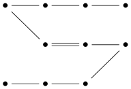
3. A Bratteli Diagram Which Is Not a Hopf–Galois Extension

We shall show that the Bratteli diagram

(7)

does not give an inclusion coming from a Hopf–Galois extension. In terms of matrices, this is

$$\begin{array}{c}\hfill \left(a\right)\oplus \left(b\right)\mapsto \left(a\right)\oplus \left(\begin{array}{cc}a& 0\\ 0& b\end{array}\right).\end{array}$$

P has a linear basis, $\left(1\right)\oplus 0$ and $\left(0\right)\oplus E_{ij}$, for $i,j\in \{0,1\}$, and A has a linear basis, $\left(1\right)\oplus E_{11}$ and $\left(0\right)\oplus E_{22}$. Note that multiplication by elements of A simply scales each of the given basis vectors in P by a number. Thus, to find $P{\otimes }_{A}P$, we only have to consider the first element of P to be a basis element. Note that in $P{\otimes }_{A}P$,

$$\begin{array}{c}\hfill (\left(1\right)\oplus 0)\otimes (\alpha \oplus \beta )=(\left(1\right)\oplus 0)(\left(1\right)\oplus E_{11})\otimes (\alpha \oplus \beta )=(\left(1\right)\oplus 0)\otimes (\left(1\right)\alpha \oplus E_{11}\beta ),\end{array}$$

so we have

$$\begin{array}{c}\hfill (\left(1\right)\oplus 0)\otimes (\left(0\right)\oplus E_{2j})=0.\end{array}$$

Next,

$$\begin{array}{c}\hfill (\left(0\right)\oplus E_{i1})\otimes (\alpha \oplus \beta )=(\left(0\right)\oplus E_{i1})(\left(1\right)\oplus E_{11})\otimes (\alpha \oplus \beta )=(\left(0\right)\oplus E_{i1})(\alpha \oplus E_{i1}\beta ),\end{array}$$

so we have

$$\begin{array}{c}\hfill (\left(0\right)\oplus E_{i1})\otimes (\left(0\right)\oplus E_{2j})=0.\end{array}$$

Next,

$$\begin{array}{c}\hfill (\left(0\right)\oplus E_{i2})\otimes (\alpha \oplus \beta )=(\left(0\right)\oplus E_{i2})(\left(0\right)\oplus E_{22})\otimes (\alpha \oplus \beta )=(\left(0\right)\oplus E_{i2})\otimes (\left(0\right)\oplus E_{22}\beta ),\end{array}$$

so we have

$$\begin{array}{c}\hfill (\left(0\right)\oplus E_{i2})\otimes (\left(1\right)\oplus 0)=(\left(0\right)\oplus E_{i2})\otimes (\left(0\right)\oplus E_{1j})=0.\end{array}$$

We have shown that 12 tensor products, on the basis of P with itself, disappear, making $P{\otimes }_{A}P$ 13-dimensional. If this was a Hopf–Galois extension this would have to be $dimP\times dimH$, which would be a multiple of 5.

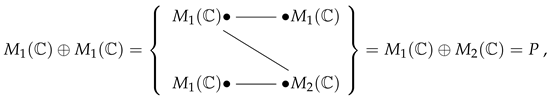
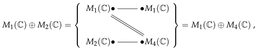
4. Combining Matrices on Block Diagonals

We consider two cases of subalgebras A of $P=M_m\left(\mathbb{C}\right)$ and also a subalgebra of the direct sum of matrix algebras, and show that they form quantum principle bundles. In the following section, we count matrices from entry 0, 0 in the top left, and use mod m arithmetic for the rows and columns of (2) and give the appropriate conditional map $M_m\left(\mathbb{C}\right)$. We follow on from the previous section by calculating $P{\otimes }_{A}P$ in the three cases.

• Case 1:

We choose block decompositions of $M_m\left(\mathbb{C}\right)$ with rows and columns divided into intervals of nonzero length $l_0, l_1, \dots , l_{n-1}$, where $l_0+l_1+\dots +l_{n-1}=m$. Let A be the image of the nonzero diagonal embedding:

$$\begin{array}{c}\hfill M_{l_0}\left(\mathbb{C}\right)\oplus M_{l_1}\left(\mathbb{C}\right)\oplus \dots \oplus M_{l_{n-1}}\left(\mathbb{C}\right)⟶M_m\left(\mathbb{C}\right).\end{array}$$

(8)

For a row or column j, we take $\left(j\right)\in {\mathbb{Z}}_n$ to be the block to which the row or column j belongs. Thus, for $n=2$, $l_0=2, l_1=1, m=3$, we have $\left(\begin{array}{ccc}a& b& 0\\ c& d& 0\\ ine0& 0& e\end{array}\right)\in A$ and $\left(0\right)=0$, $\left(1\right)=0$, $\left(2\right)=1$.

Proposition 1.

There is an isomorphism $T:M_m\left(\mathbb{C}\right){\otimes }_A{M}_m\left(\mathbb{C}\right)\to M_m\left(\mathbb{C}\right)\otimes \mathbb{C}\left[{\mathbb{Z}}_n\right]$ of $M_m\left(\mathbb{C}\right)$ bimodules which is given by

$$\begin{array}{c}\hfill T(E_{ij}\otimes E_{ab})=E_{ib}{\delta }_{ja}\otimes {\delta }_{\left(j\right)}.\end{array}$$

Here A is an image of the map in (8), and the $M_m\left(\mathbb{C}\right)$ bimodule structure on $M_m\left(\mathbb{C}\right)\otimes \mathbb{C}\left[{\mathbb{Z}}_n\right]$ involves a left and a right multiplication on the first tensor factor.

Proof. 

First, note that T is surjective, simply by choosing appropriate values of $i, b$ and $j=a$. Next, as $E_{aa}\in A$,

$$\begin{array}{c}\hfill E_{ij}\otimes E_{ab}=E_{ij}\otimes E_{aa}{E}_{ab}=E_{ij}{E}_{aa}\otimes E_{ab}={\delta }_{ja}{E}_{ij}\otimes E_{ab},\end{array}$$

so $E_{ij}\otimes E_{ab}=0$ unless $j=a$. If $\left(k\right)=\left(j\right)$, then $E_{kj}\in A$, so

$$\begin{array}{c}\hfill E_{ij}\otimes E_{jr}=E_{ik}{E}_{kj}\otimes E_{jr}=E_{ik}\otimes E_{kj}{E}_{jr}=E_{ik}\otimes E_{kr}.\end{array}$$

Thus all the $E_{ij}\otimes E_{jr}$ outcomes which have the same value of T are identified by ${\otimes }_A$. □

• Case 2:

We take the embedding $M_k\left(\mathbb{C}\right)⟶M_m\left(\mathbb{C}\right)$, where $m=nk$, sending the matrix x to the block diagonal matrix with all diagonal blocks being x, and let A be the image. For example, for $n=3$, we have

$$\begin{array}{c}\hfill \left(\begin{array}{cc}a& b\\ c& d\end{array}\right)\mapsto \left(\begin{array}{cccccc}a& b& & & & \\ c& d& & & & \\ \hfill ine\hfill & & a& b& & \\ & & c& d& & \\ \hfill ine\hfill & & & & a& b\\ & & & & c& d\end{array}\right),\hfill \end{array}$$

(9)

and we define $\left(i\right)$ as the block to which row i belongs, so $\left(0\right)=\left(1\right)=0$, $\left(2\right)=\left(3\right)=1$ and $\left(4\right)=\left(5\right)=2$. This corresponds to the notation in Case 1.

Proposition 2.

$M_m\left(\mathbb{C}\right){\otimes }_A{M}_m\left(\mathbb{C}\right)$, where A is an image of the above map, and $M_k\left(\mathbb{C}\right)⟶M_m\left(\mathbb{C}\right)$ is given by the isomorphism of $M_m\left(\mathbb{C}\right)$-$M_m\left(\mathbb{C}\right)$ bimodules $R:M_m\left(\mathbb{C}\right){\otimes }_A{M}_m\left(\mathbb{C}\right)⟶M_m\left(\mathbb{C}\right)\otimes \mathbb{C}\left[{\mathbb{Z}}_n\right]\otimes \mathbb{C}\left[{\mathbb{Z}}_n\right]$, which is given by

$$R(E_{ij}\otimes E_{ab})=\left\{\begin{array}{cc}{E}_{ib}\otimes {\delta }_r\otimes {\delta }_{\left(a\right)}\hfill & ifj=a+krmodm,\mathit{for}0\le r<n,\hfill \\ 0\hfill & otherwise.\hfill \end{array}\right.$$

Proof. 

Setting ${\displaystyle y=\sum _{0\le r<n}{E}_{a+kr,a+kr}\in A}$, we have

$$\begin{array}{c}\hfill E_{ij}\otimes E_{ab}=E_{ij}\otimes y{E}_{ab}=E_{ij}y\otimes E_{ab}.\end{array}$$

Thus, $E_{ij}\otimes E_{ab}=0$ unless $j=a+kr$ mod m for some $0\le r<n$. Now, A has linear basis ${\displaystyle \sum _{0\le r<n}{E}_{a+kr,d+kr}=G_{ad}}$ for $\left(a\right)=\left(d\right)$, i.e., a and d in the same block. Then, if $j=a+kr$ with $0\le j<m$,

$$\begin{array}{c}\hfill E_{ij}\otimes E_{ab}=E_{ij}\otimes G_{ad}{E}_{db}=E_{ij}{G}_{ad}\otimes E_{db}=E_{ij}{E}_{a+kr,d+kr}\otimes E_{db}=E_{i,d+kr}\otimes E_{db}.\end{array}$$

So, the tensor products of $E_{ij}$ have the following relation, where $\left(a\right)=\left(d\right)$,

$$\begin{array}{c}\hfill E_{i,a+kr}\otimes E_{ab}=E_{i,d+kr}\otimes E_{db}.\end{array}$$

Thus, we have r, and $\left(a\right)$ and $E_{ib}$ are the same on both sides of the relation, so R is well defined. □

• Case 3:

For unital algebra B, consider the replication map $\mathrm{rep}:B\to B^{\oplus n}=P$ given by

$$\begin{array}{c}\hfill \mathrm{rep}\left(b\right)=b\oplus \dots \oplus b,\end{array}$$

and call its image A. We write elements of $B^{\oplus n}$ as $(b_0,\dots ,b_{n-1})$. This has a module basis ${\eta }_i=(0, ,0, ,1, ,0, ,\dots , ,0)$, where 1 is in the ith position for $i\in {\mathbb{Z}}_n$. Then, for $b,c\in B$,

$$b{\eta }_i\otimes c{\eta }_j=b{\eta }_i\otimes \underline{a}.{\eta }_j,$$

where $\underline{a}=(c, ,c, ,c, ,\dots , ,c)\in A$. Then, in $B^{\oplus n}{\otimes }_A{B}^{\oplus n}$, we have

$$b{\eta }_i\otimes c{\eta }_j=b{\eta }_i.a\otimes {\eta }_j=bc{\eta }_i\otimes {\eta }_j.$$

Thus, we have an isomorphism $u:p\otimes p\to p\otimes \mathbb{C}\left({\mathbb{Z}}_n\right)$, where

$$u(b{\eta }_i\otimes c{\eta }_j)=bc{\eta }_i\otimes {\eta }_j.$$

5. Block Matrices and Quantum Principle Bundles

In this section we will show that the three cases in the previous section are actually examples of quantum principle bundles. In the definition of a Hopf–Galois extension, we will only need the case where $H=\mathbb{C}\left[G\right]$. If G acts on the algebra P on the left through algebra maps, i.e., $g▹\left(pq\right)=(g▹p)(g▹q)$, then we obtain a right $\mathbb{C}\left[G\right]$ comodule algebra ${\Delta }_R:P\to P\otimes H$ via the following:

$${\Delta }_R\left(p\right)=\sum _{g\in G}g▹p\otimes {\delta }_g.$$

(10)

We set $R_n$ to be the group of complex nth roots of unity, and recall that we label matrices from row and column zero.

• Case 1:

We define the group

$$G=\left\{g_w=\left(\begin{array}{cccc}1& & & \\ ine& \omega & & \\ ine& & \ddots & \\ ine& & & {\omega }^{n-1}\end{array}\right):\omega \in R_n\right\}\subset G{L}_m\left(\mathbb{C}\right),$$

(11)

using blocks of length $l_0, ,\dots l_{n-1}$, and we insert the appropriate identity matrices in the blocks. Now, G acts on $P=M_m\left(\mathbb{C}\right)$ through algebra maps $g_{\omega }▹x=g_{\omega }x{g}_{\omega }^{-1}$. For x purely in the $st$ block for $s, ,t\in {\mathbb{Z}}_n$, we have

$$\begin{array}{c}\hfill g_{\omega }▹x={\omega }^{s-t}x,\end{array}$$

so the fixed points of the G action are precisely the block-diagonal subalgebra A. The canonical map is

$$\begin{array}{c}\hfill \mathrm{can}(E_{ij}\otimes E_{ab})={\delta }_{ja}\sum _{\omega \in R_n}{E}_{ib}{\omega }^{\left(a\right)-\left(b\right)}\otimes {\delta }_{\omega }\mathrm{where}a, ,b, ,i, ,j\in {\mathbb{Z}}_m.\end{array}$$

If the canonical map is surjective, then it is automatically injective, since the dimension of $M_m\left(\mathbb{C}\right){\otimes }_A{M}_m\left(\mathbb{C}\right)$ is the same as $M_m\left(\mathbb{C}\right)\otimes H$ according to the previous section. Now, for $\xi \in R_n$,

$$\begin{array}{c}\hfill \mathrm{can}\left({\xi }^{\left(i\right)-\left(j\right)}{E}_{ij}\otimes E_{ji}\right)=\sum _{\omega \in R_n}{E}_{ii}{\left({\displaystyle \frac{\omega }{\xi }}\right)}^{\left(j\right)-\left(i\right)}\otimes {\delta }_{\omega },\end{array}$$

so

$$\begin{array}{c}\hfill \sum _{j\in {\mathbb{Z}}_m}{\displaystyle \frac{1}{l_{\left(j\right)}}}{\xi }^{\left(i\right)-\left(j\right)}\mathrm{can}\left(E_{ij}\otimes E_{ji}\right)=\sum _{q\in {\mathbb{Z}}_n,\omega \in R_n}{E}_{ii}{\left({\displaystyle \frac{\omega }{\xi }}\right)}^{q-\left(i\right)}\otimes {\delta }_{\omega },\end{array}$$

and according to the formula for the sum of a geometric progression, this sum is zero unless ${\displaystyle \frac{\omega }{\xi }}=1$. Thus,

$$\begin{array}{c}\hfill \mathrm{can}\left(\sum _{j,i\in {\mathbb{Z}}_n}{\displaystyle \frac{1}{l^{\left(j\right)}}}{\xi }^{\left(i\right)-\left(j\right)}{E}_{ij}\otimes E_{ji}\right)=n\sum _i{E}_{ii}\otimes {\delta }_{\xi }=n·I_m\otimes {\delta }_{\xi }.\end{array}$$

(12)

Since the canonical map is a left P-module map, we see that it is surjective, and we have a quantum principle bundle. We have proven the following Proposition

Proposition 3.

For $\xi \ne 1$, set

$$\begin{array}{c}\hfill {\delta }_{\xi }^{\left(1\right)}\otimes {\delta }_{\xi }^{\left(2\right)}={\displaystyle \frac{1}{n}}\sum _{j,i}{\displaystyle \frac{1}{l_{\left(j\right)}}}{\xi }^{\left(i\right)-\left(j\right)}{E}_{ij}\otimes E_{ji},{\delta }_1^{\left(1\right)}\otimes {\delta }_1^{\left(2\right)}=I_m\otimes I_m-\sum _{\xi \ne 1}{\delta }_{\xi }^{\left(1\right)}\otimes {\delta }_{\xi }^{\left(2\right)}.\end{array}$$

(13)

Then, $1^{\left(1\right)}\otimes 1^{\left(2\right)}=I_m\otimes I_m$ and for all $\eta \in R_n$.

$$\begin{array}{c}\hfill \mathrm{can}\left({\delta }_{\eta }^{\left(1\right)}\otimes {\delta }_{\eta }^{\left(2\right)}\right)=I_m\otimes {\delta }_{\eta }.\end{array}$$

(14)

• Case 2:

For $\omega \in R_n$ and $i\in {\mathbb{Z}}_n$, define them using blocks of length k as before:

$$\begin{array}{c}\hfill g_{i,\omega }=\left(\begin{array}{ccccccc}0& \cdots & 0& 1& 0& \cdots & 0\\ 0& \cdots & 0& 0& \omega & \cdots & \cdots \\ :& :& :& :& :& :& :\\ {\omega }^{n-i}& 0& 0& 0& 0& 0& 0\\ :& :& :& :& :& :& :\\ 0& \cdots & {\omega }^{n-1}& 0& 0& \cdots & 0\end{array}\right),\end{array}$$

where the original 1 (in fact, $I_k$) is in column i (counting from column 0). Note that

$$\begin{array}{c}\hfill g_{i,\omega }{g}_{j,\eta }={\eta }^i{g}_{i+j,\omega \eta },g_{i,\omega }^{-1}={\omega }^i{g}_{-i,{\displaystyle \frac{1}{\omega }}}.\end{array}$$

(15)

We take the group G of projective matrices $G\subset PG{L}_n\left(\mathbb{C}\right)$ consisting of $g_{i,\omega }$, so we obtain $G\cong {\mathbb{Z}}_n\times R_n$. Then, we define an action of G on $M_m\left(\mathbb{C}\right)$ via $(i,\omega )▹x=g_{i,\omega }x{g}_{i,\omega }^{-1}$, which is not dependent on a scale factor on the $g_{i,\omega }$ (this is why we can use the term projective above).We use $F_{jt}$ for $j, ,t\in {\mathbb{Z}}_n$ to denote the identity matrix in the $jt$ block and zero elsewhere. Now, using (10),

$$\begin{array}{c}\hfill (i,\omega )▹F_{jt}={\omega }^{j-t}{F}_{j-i,t-i},{\Delta }_R{F}_{jt}=\sum _{s,\omega }{\omega }^{j-t}{F}_{j-s,t-s}\otimes {\delta }_{(s,\omega )},\end{array}$$

and the canonical map is

$$\begin{array}{c}\hfill \mathrm{can}(F_{ab}\otimes F_{jt})=\sum _{\omega }{\omega }^{j-t}{F}_{a,t-j+b}\otimes {\delta }_{(j-b,\omega )},\end{array}$$

and a particular case of this is that by setting $b=j-i$ and $t=i+a$,

$$\begin{array}{c}\hfill \mathrm{can}(F_{a,j-i}\otimes F_{j,i+a})=\sum _{\omega }{\omega }^{j-i-a}{F}_{a,a}\otimes {\delta }_{(i,\omega )}.\end{array}$$

Now, using the sum of powers of a root of unity,

$$\begin{array}{c}\hfill \mathrm{can}\left(\sum _j{\xi }^{i-j}(F_{a,j-i}\otimes F_{j,i+a})\right)=\sum _{\omega ,j}{\omega }^{-a}{\left({\displaystyle \frac{\omega }{\xi }}\right)}^{j-i}{F}_{a,a}\otimes {\delta }_{(i,\omega )}=n{\xi }^{-a}{F}_{a,a}\otimes {\delta }_{(i,\xi )},\end{array}$$

so

$$\begin{array}{c}\hfill \mathrm{can}\left(\sum _{j,a}{\displaystyle \frac{1}{n}}{\xi }^{i-j+a}(F_{a,j-i}\otimes F_{j,i+a})\right)=\sum _a{F}_{a,a}\otimes {\delta }_{(i,\xi )}=I_m\otimes {\delta }_{(i,\xi )}.\end{array}$$

(16)

Thus, we have proven the following Proposition:

Proposition 4.

If we define, for $(i,\xi )\ne (0,1)$,

$$\begin{array}{c}\hfill {\delta }_{(i,\xi )}^{\left(1\right)}\otimes {\delta }_{(i,\xi )}^{\left(2\right)}={\displaystyle \frac{1}{n}}\sum _{j,a}{\xi }^{i-j+a}{F}_{a,j-i}\otimes F_{j,i+a},{\delta }_{(0,1)}^{\left(1\right)}\otimes {\delta }_{(0,1)}^{\left(2\right)}=I_m\otimes I_m-\sum _{(i,\xi )\ne (0,1)}{\delta }_{(i,\xi )}^{\left(1\right)}\otimes {{\delta }_{(i,\xi )}}^{\left(2\right)},\end{array}$$

(17)

then $1^{\left(1\right)}\otimes 1^{\left(2\right)}=I_m\otimes I_m$, and for all $(j,\eta )\in {\mathbb{Z}}_n\times R_n$,

$$\begin{array}{c}\hfill \mathrm{can}\left({\delta }_{(j,\eta )}^{\left(1\right)}\otimes {\delta }_{(j,\eta )}^{\left(2\right)}\right)=I_m\otimes {\delta }_{(j,\eta )}.\end{array}$$

(18)

• Case 3:

We use the group $G={\mathbb{Z}}_n$ acting on $P=B^{\oplus n}$ via $i▹{\eta }_s={\eta }_{s+i}modn$. Now,

$$\begin{array}{c}\hfill \mathrm{can}({\eta }_t\otimes {\eta }_s)={\eta }_t.\sum _{i\in {\mathbb{Z}}_n}{\eta }_{s+i}\otimes {\delta }_i={\eta }_t\otimes {\delta }_{t-s},\end{array}$$

(19)

so we have the following Proposition.

Proposition 5.

If we define, for $i\in {\mathbb{Z}}_n$,

$$\begin{array}{c}\hfill {\delta }_i^{\left(1\right)}\otimes {\delta }_i^{\left(2\right)}=\sum _t{\eta }_t\otimes {\eta }_{t-i},\end{array}$$

(20)

then $1^{\left(1\right)}\otimes 1^{\left(2\right)}={\sum }_t{\eta }_t\otimes {\sum }_s{\eta }_s$ and

$$\begin{array}{c}\hfill \mathrm{can}\left({\delta }_i^{\left(1\right)}\otimes {\delta }_i^{\left(2\right)}\right)=\sum _t{\eta }_t\otimes {\delta }_i.\end{array}$$

(21)

6. Strong Universal Connection

We find the strong universal connections corresponding to the cases in the previous section, starting with the back maps $h\mapsto h^{\left(1\right)}\otimes h^{\left(2\right)}$ given there. Note these have been defined so that $1^{\left(1\right)}\otimes 1^{\left(2\right)}=1\otimes 1$. This uses Theorem 1 and the normalised integral on $\mathbb{C}\left[G\right]$ for G a finite group ${\displaystyle \int f={\displaystyle \frac{1}{\left|G\right|}}\sum _{g\in G}f\left(g\right)}$.

Proposition 6.

In Case 1,

$$\begin{array}{c}\hfill {\omega }^{♯}\left({\delta }_{\eta }\right)={\displaystyle \frac{1}{n}}\sum _{i,j\in {\mathbb{Z}}_m:\left(i\right)\ne \left(j\right)}{\displaystyle \frac{1}{l^{\left(j\right)}}}{\eta }^{\left(i\right)-\left(j\right)}{E}_{ij}\otimes E_{ji}+{\displaystyle \frac{1}{n}}{I}_m\otimes I_m.\end{array}$$

(22)

Proof. 

According to Theorem 1 and Proposition 3,

$$\begin{array}{cc}\hfill {\omega }^{♯}\left({\delta }_{\eta }\right)& =\sum _{\omega ,\xi }{a}_L({\delta }_{\omega }\otimes {\delta }_{\xi }^{\left(1\right)})\otimes a_R({\delta }_{\xi }^{\left(2\right)}\otimes {\delta }_{\eta {\omega }^{-1}{\xi }^{-1}})\hfill \\ \hfill & =\sum _{\omega ,\xi \ne 1}{a}_L({\delta }_{\omega }\otimes {\delta }_{\xi }^{\left(1\right)})\otimes a_R({\delta }_{\xi }^{\left(2\right)}\otimes {\delta }_{\eta {\omega }^{-1}{\xi }^{-1}})+\sum _{\omega }{a}_L({\delta }_{\omega }\otimes I_m)\otimes a_R(I_m\otimes {\delta }_{\eta {\omega }^{-1}})\hfill \\ \hfill & -\sum _{\omega ,\xi \ne 1}{a}_L({\delta }_{\omega }\otimes {\delta }_{\xi }^{\left(1\right)})\otimes a_R({\delta }_{\xi }^{\left(2\right)}\otimes {\delta }_{\eta {\omega }^{-1}})\hfill \\ \hfill & =\sum _{\omega ,\xi \ne 1}{a}_L({\delta }_{\omega }\otimes {\delta }_{\xi }^{\left(1\right)})\otimes a_R({\delta }_{\xi }^{\left(2\right)}\otimes ({\delta }_{\eta {\omega }^{-1}{\xi }^{-1}}-{\delta }_{\eta {\omega }^{-1}}))+\sum _{\omega }{a}_L({\delta }_{\omega }\otimes I_m)\otimes a_R(I_m\otimes {\delta }_{\eta {\omega }^{-1}})\hfill \\ \hfill & ={\displaystyle \frac{1}{n}}\sum _{\omega ,\xi \ne 1,i,j}{\displaystyle \frac{1}{l^{\left(j\right)}}}{\xi }^{\left(i\right)-\left(j\right)}{a}_L({\delta }_{\omega }\otimes E_{ij})\otimes a_R\left(E_{ji}\otimes ({\delta }_{\eta {\omega }^{-1}{\xi }^{-1}}-{\delta }_{\eta {\omega }^{-1}})\right)\hfill \\ \hfill & +\sum _{\omega }{a}_L({\delta }_{\omega }\otimes I_m)\otimes a_R(I_m\otimes {\delta }_{\eta {\omega }^{-1}}).\hfill \end{array}$$

Then, we calculate $a_R$ and $a_L$ for both sums via $a_R(E_{ij}\otimes {\delta }_{\xi })={\displaystyle \frac{1}{n}}{\xi }^{\left(j\right)-\left(i\right)}{E}_{ij}$ and $a_L({\delta }_{\xi }\otimes E_{ij})={\displaystyle \frac{1}{n}}{\xi }^{\left(i\right)-\left(j\right)}{E}_{ij}$, and so,

$$\begin{array}{cc}\hfill {\omega }^{♯}\left({\delta }_{\eta }\right)& ={\displaystyle \frac{1}{n^3}}\sum _{\omega ,\xi \ne 1,i,j}{\displaystyle \frac{1}{l^{\left(j\right)}}}{\xi }^{\left(i\right)-\left(j\right)}{\omega }^{\left(i\right)-\left(j\right)}{E}_{ij}\otimes E_{ji}\left({\left(\eta {\omega }^{-1}{\xi }^{-1}\right)}^{\left(i\right)-\left(j\right)}-{\left(\eta {\omega }^{-1}\right)}^{\left(i\right)-\left(j\right)}\right)\hfill \\ \hfill & +\sum _{\omega ,i}{\displaystyle \frac{1}{n}}{E}_{ii}\otimes \sum _i{\displaystyle \frac{1}{n}}{E}_{ii}\hfill \\ \hfill & ={\displaystyle \frac{1}{n^3}}\sum _{\omega ,\xi \ne 1,i,j}{\displaystyle \frac{1}{l^{\left(j\right)}}}{\xi }^{\left(i\right)-\left(j\right)}{\eta }^{\left(i\right)-\left(j\right)}\left({\xi }^{\left(j\right)-\left(i\right)}-1\right)E_{ij}\otimes E_{ji}+\sum _{\omega }{\displaystyle \frac{1}{n^2}}{I}_m\otimes I_m\hfill \\ \hfill & ={\displaystyle \frac{1}{n^2}}\sum _{\xi \ne 1,i,j}{\displaystyle \frac{1}{l^{\left(j\right)}}}{\eta }^{\left(i\right)-\left(j\right)}{E}_{ij}\otimes E_{ji}\left(1-{\xi }^{\left(i\right)-\left(j\right)}\right)+{\displaystyle \frac{1}{n}}{I}_m\otimes I_m.\hfill \end{array}$$

(23)

Now, for the first term, if $\left(i\right)-\left(j\right)\ne 0$, we obtain

$$\begin{array}{c}\hfill \sum _{\xi }{\xi }^{\left(i\right)-\left(j\right)}=0=1+\sum _{\xi \ne 1}{\xi }^{\left(i\right)-\left(j\right)}.\end{array}$$

(24)

We split the last equation in (23) into an $\left(i\right)=\left(j\right)$ part (the summand vanishes) and $\left(i\right)\ne \left(j\right)$ part, where summing over $\xi$ and using (24) gives

$$\begin{array}{c}\hfill {\omega }^{♯}\left({\delta }_{\eta }\right)={\displaystyle \frac{1}{n^2}}\sum _{i,j:\left(i\right)\ne \left(j\right)}{\displaystyle \frac{1}{l^{\left(j\right)}}}{\eta }^{\left(i\right)-\left(j\right)}{E}_{ij}\otimes E_{ji}\left(n-1+1\right)={\displaystyle \frac{1}{n}}\sum _{i,j:\left(i\right)\ne \left(j\right)}{\displaystyle \frac{1}{l^{\left(j\right)}}}{\eta }^{\left(i\right)-\left(j\right)}{E}_{ij}\otimes E_{ji}.\end{array}$$

□

Proposition 7.

In Case 2,

$$\begin{array}{c}\hfill {\omega }^{♯}\left({\delta }_{(k,\eta )}\right)={\displaystyle \frac{1}{n}}\sum _{b,s\in {\mathbb{Z}}_m}{\eta }^{b-s}{F}_{b,s}\otimes F_{s+k,b+k}-{\displaystyle \frac{1}{n^2}}\sum _{b,i\in {\mathbb{Z}}_m}{F}_{b,b}\otimes F_{i+k+b,i+k+b}.\end{array}$$

(25)

Proof. 

According to Proposition 4,

$$\begin{array}{cc}\hfill {\omega }^{♯}\left({\delta }_{(k,\eta )}\right)& =\sum _{(i,p,\omega ,\xi )}{a}_L\left({\delta }_{(p,\omega )}\otimes {\delta }_{(i,\xi )}^{\left(1\right)}\right)\otimes a_R\left({\delta }_{(i,\xi )}^{\left(2\right)}\otimes {\delta }_{(k-p-i,\eta {\omega }^{-1}{\xi }^{-1})}\right)\hfill \\ \hfill & =\sum _{(p,\omega ),(i,\xi )\ne (0,1)}{a}_L\left({\delta }_{(p,\omega )}\otimes {\delta }_{(i,\xi )}^{\left(1\right)}\right)\otimes a_R\left({\delta }_{(i,\xi )}^{\left(2\right)}\otimes {\delta }_{(k-p-i,\eta {\omega }^{-1}{\xi }^{-1})}\right)\hfill \\ \hfill & +\sum _{(p,\omega )}{a}_L\left({\delta }_{(p,\omega )}\otimes {\delta }_{(0,1)}^{\left(1\right)}\right)\otimes a_R\left({\delta }_{(0,1)}^{\left(2\right)}\otimes {\delta }_{(k-p,\eta {\omega }^{-1})}\right)\hfill \\ \hfill & =\sum _{(p,\omega ),(i,\xi )\ne (0,1)}{a}_L\left({\delta }_{(p,\omega )}\otimes {\delta }_{(i,\xi )}^{\left(1\right)}\right)\otimes a_R\left({\delta }_{(i,\xi )}^{\left(2\right)}\otimes ({\delta }_{(k-p-i,\eta {\omega }^{-1}{\xi }^{-1})}-{\delta }_{(k-p,\eta {\omega }^{-1})})\right)\hfill \\ \hfill & +\sum _{(p,\omega )}{a}_L\left({\delta }_{(p,\omega )}\otimes I_m\right)\otimes a_R\left(I_m\otimes {\delta }_{(k-p,\eta {\omega }^{-1})}\right).\hfill \end{array}$$

Using $a_R(F_{jk}\otimes {\delta }_{(r,\xi )})={\displaystyle \frac{1}{n^2}}{\xi }^{k-j}{F}_{j+r,k+r}$ and $a_L({\delta }_{(r,\xi )}\otimes F_{jk})={\displaystyle \frac{1}{n^2}}{\xi }^{j-k}{F}_{j-r,k-r}$ for both terms,

$$\begin{array}{cc}\hfill & ={\displaystyle \frac{1}{n}}\sum _{(p,\omega ),(i,\xi )\ne (0,1),j,a}{a}_L\left({\delta }_{(p,\omega )}\otimes {\xi }^{i-j+a}{F}_{a,j-i}\right)\otimes a_R\left(F_{j,i+a}\otimes ({\delta }_{(k-p-i,\eta {\omega }^{-1}{\xi }^{-1})}-{\delta }_{(k-p,\eta {\omega }^{-1})})\right)\hfill \\ \hfill & ={\displaystyle \frac{1}{n^5}}\sum _{(p,\omega ),(i,\xi )\ne (0,1),j,a}\left({\xi }^{i-j+a}{\omega }^{a-j+i}{F}_{a-p,j-i-p}\right)\otimes \hfill \\ & \left({\left(\eta {\omega }^{-1}{\xi }^{-1}\right)}^{i+a-j}{F}_{j+k-p-i,i+a+k-p-i}-{\left(\eta {\omega }^{-1}\right)}^{i+a-j}{F}_{j+k-p,i+a+k-p}\right)\hfill \\ \hfill & ={\displaystyle \frac{1}{n^4}}\sum _{p,j,a,(i,\xi )\ne (0,1)}{\left(\xi \eta \right)}^{i+a-j}{F}_{a-p,j-i-p}\otimes \left({\xi }^{j-i-a}{F}_{j+k-p-i,a+k-p}-F_{j+k-p,i+a+k-p}\right)\hfill \\ \hfill & ={\displaystyle \frac{1}{n^4}}\sum _{p,j,a,i\ne 0,\xi }{\eta }^{i+a-j}{F}_{a-p,j-i-p}\otimes \left(F_{j+k-p-i,a+k-p}-{\xi }^{i+a-j}{F}_{j+k-p,i+a+k-p}\right)\hfill \\ \hfill & +{\displaystyle \frac{1}{n^4}}\sum _{p,j,a,\xi \ne 1}{\eta }^{a-j}{F}_{a-p,j-p}\otimes F_{j+k-p,a+k-p}\left(1-{\xi }^{a-j}\right).\hfill \end{array}$$

(26)

The first part of Equation (26) is

$$\begin{array}{cc}\hfill & ={\displaystyle \frac{1}{n^3}}\sum _{p,j,a,i\ne 0}{\eta }^{i+a-j}{F}_{a-p,j-i-p}\otimes \left(F_{j+k-p-i,a+k-p}-{\delta }_{i+a-j,0}{F}_{j+k-p,i+a+k-p}\right)\hfill \\ \hfill & ={\displaystyle \frac{1}{n^3}}\sum _{p,j,a,i\ne 0}{\eta }^{i+a-j}{F}_{a-p,j-i-p}\otimes F_{j+k-p-i,a+k-p}-{\displaystyle \frac{1}{n^3}}\sum _{p,a,i\ne 0}{F}_{a-p,a-p}\otimes F_{i+a+k-p,i+a+k-p}\hfill \\ \hfill & ={\displaystyle \frac{n-1}{n^3}}\sum _{p,s,a}{\eta }^{a-s}{F}_{a-p,s-p}\otimes F_{s+k-p,a+k-p}-{\displaystyle \frac{1}{n^3}}\sum _{p,a,i\ne 0}{F}_{a-p,a-p}\otimes F_{i+a+k-p,i+a+k-p}\hfill \\ \hfill & ={\displaystyle \frac{n-1}{n^2}}\sum _{b,r}{\eta }^{b-r}{F}_{b,r}\otimes F_{r+k,b+k}-{\displaystyle \frac{1}{n^2}}\sum _{b,i\ne 0}{F}_{b,b}\otimes F_{i+k+b,i+k+b},\hfill \end{array}$$

(27)

where we have relabelled $s=j-i$ in the first term. Next, we relabel $b=a-p$ and $r=s-p$. Now, let $b=a-p$ and $s=j-p$ in the second part of (26),

$$\begin{array}{cc}\hfill {\displaystyle \frac{1}{n^4}}\sum _{p,s,b,\xi \ne 1}{\eta }^{b-s}{F}_{b,s}\otimes F_{s+k,b+k}\left(1-{\xi }^{b-s}\right)& ={\displaystyle \frac{1}{n^3}}\sum _{s,b,\xi \ne 1}{\eta }^{b-s}{F}_{b,s}\otimes F_{s+k,b+k}\left(1-{\xi }^{b-s}\right)\hfill \\ \hfill & ={\displaystyle \frac{1}{n^2}}\sum _{s,b}{\eta }^{b-s}{F}_{b,s}\otimes F_{s+k,b+k}\left(1-{\delta }_{b,s}\right),\hfill \end{array}$$

(28)

since ${\displaystyle \sum _{\xi \ne 1}\left(1-{\xi }^{b-s}\right)=n(1-{\delta }_{b,s})}$, and adding Equations (27) and (28) gives the results. □

Proposition 8.

In Case 3,

$$\begin{array}{c}\hfill {\omega }^{♯}\left({\delta }_i\right)=\sum _{s\in {\mathbb{Z}}_n}{\delta }_s\otimes {\delta }_{s-i}.\end{array}$$

(29)

Proof. 

From Theorem 1 and (20),

$$\begin{array}{c}\hfill {\omega }^{♯}\left({\delta }_i\right)=\sum _{j,k}{a}_L({\delta }_j\otimes {{\delta }_k}^{\left(1\right)})\otimes a_R({{\delta }_k}^{\left(2\right)}\otimes {\delta }_{i-j-k})=\sum _{j,k,t}{a}_L({\delta }_j\otimes {\eta }_t)\otimes a_R({\eta }_{t-k}\otimes {\delta }_{i-j-k}).\end{array}$$

As ${\displaystyle {\Delta }_R{b}_{,t}=\sum _s{b}_{t+s}\otimes {\delta }_s}$,

$$\begin{array}{cc}\hfill a_L({\delta }_j\otimes {\eta }_t)& =\sum _{s}b({\delta }_j\otimes {\delta }_{-s}){\eta }_{t+s}=\sum _s(\int {\delta }_j{\delta }_s){\eta }_{t+s}={\displaystyle \frac{1}{n}}{\eta }_{t+j},\hfill \\ \hfill a_R({\eta }_t\otimes {\delta }_j)& =\sum _s{\eta }_{t+s}b({\delta }_s\otimes {\delta }_j)=\sum _s(\int {\delta }_s{\delta }_{-j}){\eta }_{t+s}={\displaystyle \frac{1}{n}}{\eta }_{t-j},\hfill \end{array}$$

so

$$\begin{array}{c}\hfill {\omega }^{♯}\left({\delta }_i\right)={\displaystyle \frac{1}{n^2}}\sum _{j,k,t}{\eta }_{t+j}\otimes {\eta }_{t-i+j}={\displaystyle \frac{1}{n}}\sum _{j,t}{\eta }_{t+j}\otimes {\eta }_{t-i+j}.\end{array}$$

(30)

Setting $s=t+j$ gives the answer. □

7. A Trivial Quantum Principle Bundle

We first recall that if $\Phi ,\Psi$ are maps from a coalgebra (in our case, H) to an algebra, then so is the convolution product ⊙ defined by

$$\Phi \odot \Psi =·(\Phi \otimes \Psi )\Delta ,$$

and that $\Phi$ is convolution-invertible when there is an inverse ${\Phi }^{-1}$ such that $\Phi \odot {\Phi }^{-1}={\Phi }^{-1}\odot \Phi =1.ϵ$.

Proposition 9

([10], Section 5.1.2). Let P be a right H-comodule algebra equipped with a convolution-invertible right-comodule map $\Phi :H\to P$ with $\Phi \left(1\right)=1$. Then, P is a quantum principal bundle over $A=P^H$. We call it a trivial bundle with trivialisation Φ.

We show that the algebra $M_n\left(\mathbb{C}\right)$ is a trivial Hopf–Galois extension of the group ${\mathbb{Z}}_n\times {\mathbb{Z}}_n$, referring to the construction in Section 5, Case 2. We use the notation $R_n$ to be the multiplicative group of the nth roots of unity, generated by $x=e^{2\pi i/n}$ with $x^n=1$.

Proposition 10.

The construction of Section 5, Case 2, gives a trivial quantum principle bundle with algebra $P=M_n\left(\mathbb{C}\right)$ and Hopf algebra $H=\mathbb{C}\left[G\right]$ for $G={\mathbb{Z}}_n\times R_n$.

Proof. 

We start by defining ${\displaystyle \Phi \left({\delta }_{(s,\omega )}\right)=\sum _{ij}{\Phi }_{s,\omega ,i,j}{F}_{ij}}$ as a right comodule map, meaning the following quantities are equal:

$$\begin{array}{cc}\hfill {\Delta }_R\Phi \left({\delta }_{(s,\omega )}\right)& =\sum _{i,j,r,\xi }{\Phi }_{s,\omega ,i,j}{\xi }^{i-j}{F}_{i-r,j-r}\otimes {\delta }_{(r,\xi )},\hfill \\ \hfill (\Phi \otimes \mathrm{id})\Delta \left({\delta }_{(s,\omega )}\right)& =\sum _{t,\eta }\Phi \left({\delta }_{(t,\eta )}\right)\otimes {\delta }_{(s-t,{\displaystyle \frac{\omega }{\eta }})}=\sum _{t,\eta ,p,q}{\Phi }_{t,\eta ,p,q}{F}_{pq}\otimes {\delta }_{(s-t,{\displaystyle \frac{\omega }{\eta }})}.\hfill \end{array}$$

(31)

Using these, we can show that there is ${\beta }_{ij}$ with

$$\begin{array}{c}\hfill {\Phi }_{s,\omega ,i,j}={\omega }^{j-i}{\beta }_{i-s,j-s},\end{array}$$

and for $\Phi \left(1\right)=1$, we need ${\displaystyle \sum _i{\beta }_{ii}=\frac{1}{n}}$. The inverse $\Psi$ of $\Phi$ in Proposition 9 can be shown to obey ${\Delta }_R\Psi \left(h\right)=\Psi \left(h_{\left(2\right)}\right)\otimes S{h}_{\left(1\right)}$. Writing $\Psi$ as ${\displaystyle \Psi \left({\delta }_{(s,\omega )}\right)=\sum _{ij}{\Psi }_{s,\omega ,i,j}{F}_{ij}}$, we can show that ${\Psi }_{s,\omega ,i,j}={\omega }^{i-j}{\gamma }_{i+s,j+s}$. The equations for convolution inverse reduce to

$${\eta }^{j-i}{\beta }_{i-t,j-t}{\left({\displaystyle \frac{\omega }{\eta }}\right)}^{j-q}{\gamma }_{j+s-t,q+s-t}{F}_{iq}=\left\{\begin{array}{cc}{I}_n\hfill & \mathrm{i}\mathrm{f}s=0\mathrm{and}\omega =1,\hfill \\ 0\hfill & \mathrm{o}\mathrm{t}\mathrm{h}\mathrm{e}\mathrm{r}\mathrm{w}\mathrm{i}\mathrm{s}\mathrm{e}.\hfill \end{array}\right.$$

Thus, explicitly summing for clarity,

$$\sum _{t,\eta ,j}{\omega }^{j-q}{\eta }^{q-i}{\beta }_{i-t,j-t}{\gamma }_{j+s-t,q+s-t}=\left\{\begin{array}{cc}{\delta }_{iq}\hfill & \mathrm{i}\mathrm{f}s=0\mathrm{and}\omega =1,\hfill \\ 0\hfill & \mathrm{o}\mathrm{t}\mathrm{h}\mathrm{e}\mathrm{r}\mathrm{w}\mathrm{i}\mathrm{s}\mathrm{e}.\hfill \end{array}\right.$$

The sum over $\eta$ gives zero unless $q=i$, so we are left with

$$n\sum _j{\omega }^{j-i}\sum _t{\beta }_{i-t,j-t}{\gamma }_{j+s-t,i+s-t}=\left\{\begin{array}{cc}1\hfill & \mathrm{i}\mathrm{f}s=0\mathrm{and}\omega =1,\hfill \\ 0\hfill & \mathrm{o}\mathrm{t}\mathrm{h}\mathrm{e}\mathrm{r}\mathrm{w}\mathrm{i}\mathrm{s}\mathrm{e}.\hfill \end{array}\right.$$

Now, we use the result that the evaluation gives, an isomorphism from $\mathbb{C}{\left[\omega \right]}_{<n}$ (the polynomials of degree $<nmodn$) to $\mathbb{C}\left[R_n\right]$, to obtain the complex functions on the set $R_n$ (a version of the discrete Fourier transform). Using this, we can rewrite (7) as

$$\sum _t{\beta }_{i-t,j-t}{\gamma }_{j+s-t,i+s-t}=\left\{\begin{array}{cc}{\displaystyle \frac{1}{n^2}}\hfill & \mathrm{i}\mathrm{f}s=0,\hfill \\ 0\hfill & \mathrm{o}\mathrm{t}\mathrm{h}\mathrm{e}\mathrm{r}\mathrm{w}\mathrm{i}\mathrm{s}\mathrm{e}.\hfill \end{array}\right.$$

Let $r=i-t$ so $t=i-r$ and $k=j-i$; then, for k and s,

$$\sum _r{\beta }_{r,r+k}{\gamma }_{s+r+k,s+r}=\left\{\begin{array}{cc}{\displaystyle \frac{1}{n^2}}\hfill & \mathrm{i}\mathrm{f}s=0,\hfill \\ 0\hfill & \mathrm{o}\mathrm{t}\mathrm{h}\mathrm{e}\mathrm{r}\mathrm{w}\mathrm{i}\mathrm{s}\mathrm{e}.\hfill \end{array}\right.$$

(32)

The values ${\beta }_{0,k}={\displaystyle \frac{1}{n}}$ and ${\gamma }_{k,0}={\displaystyle \frac{1}{n}}$ for all $k\in {\mathbb{Z}}_n$ with all other ${\beta }_{ij}$ and ${\gamma }_{ij}$ having values of zero solve (32), and also ${\displaystyle \sum _i{\beta }_{ii}=\frac{1}{n}}$. Thus, we have a trivial Hopf–Galois extension. □

8. Consequences for Differential Calculus

We can use Hopf–Galois extensions to study differential calculi on algebras. In particular we have the idea of a quantum principle bundle where we have the exact sequence

$$\begin{array}{c}\hfill 0⟶P{\Omega }_A^{1}P\stackrel{\mathrm{inc}}{\to }{\Omega }_P^1\stackrel{\mathrm{ver}}{\to }P\otimes {\Lambda }_H^1⟶0,\end{array}$$

(33)

where $\mathrm{inc}$ is the inclusion map and ${\Lambda }_H^1$ is the left invariant 1-forms on H. The vertical map is defined by

$$\begin{array}{c}\hfill \mathrm{ver}(p.\mathrm{d}q)=p{q}_{\left[0\right]}\otimes S\left(q_{\left[1\right]}\right)\mathrm{d}{q}_{\left[2\right]},\end{array}$$

and is well defined if the map $p.\mathrm{d}q\mapsto p_{\left[0\right]}{q}_{\left[0\right]}\otimes p_{\left[1\right]}\mathrm{d}{q}_{\left[1\right]}$ from ${\Omega }_P^1$ to $P\otimes {\Omega }_H^1$ is well defined. This condition can be thought of as H coacting on P in a differentiable manner.

We shall use this theory to build calculi for matrices $M_n\left(\mathbb{C}\right)$ from calculi on groups. We take Case 2 of our previous discussion, where $A=M_1\left(\mathbb{C}\right)$ and $P=M_n\left(\mathbb{C}\right)$. As $\mathrm{d}1=0$, A must have the zero calculus, and (33) becomes

$$\begin{array}{c}\hfill 0⟶0⟶{\Omega }_P^1\stackrel{\mathrm{ver}}{\to }P\otimes {\Lambda }_H^1⟶0,\end{array}$$

so the left module map $\mathrm{ver}$ is an isomorphism. If we write $\mathrm{ver}\left(\xi \right)={\xi }^0\otimes {\xi }^1$, then

$$\begin{array}{c}\hfill \mathrm{ver}\left(p\xi \right)=p{\xi }^0\otimes {\xi }^1\mathrm{and}\mathrm{ver}\left(\xi p\right)={\xi }^0{p}_{\left[0\right]}\otimes {\xi }^1◃p_{\left[1\right]},\end{array}$$

(34)

where $\eta ◃h=S\left(h_{\left(1\right)}\right)\eta h_{\left(2\right)}$. The first-order left covariant differential calculi on $H=\mathbb{C}\left[G\right]$ for a finite group G correspond to subsets $\mathcal{C}\subseteq G\setminus \left\{e\right\}$ [10], Section 1.7. The basis as a left module for the left invariant 1-forms is $e_a$ for $a\in \mathcal{C}$, with the relations and exterior derivative for $f\in \mathbb{C}\left[G\right]$ being

$$e_a.f=R_a\left(f\right)e_a,\mathrm{d}f=\sum _{a\in \mathcal{C}}(R_a\left(f\right)-f)e_a,$$

where $R_a\left(f\right)=f\left(\left(\right)a\right)$ denotes right-translation. We can calculate

$$\begin{array}{cc}\hfill \mathrm{ver}\left(\mathrm{d}p\right)& =\sum _{g\in G}g▹p\otimes S\left({\delta }_{g_{\left(1\right)}}\right)\mathrm{d}{\delta }_{g_{\left(2\right)}}\hfill \\ \hfill & =\sum _{g,x,y\in G:xy=g}\sum _{a\in \mathcal{C}}g▹p\otimes {\delta }_{x^{-1}}({\delta }_{y{a}^{-1}}-{\delta }_y)e_a\hfill \\ \hfill & =\sum _{a\in \mathcal{C}}\sum _{x,g\in \mathcal{C}}g▹p\otimes {\delta }_{x^{-1}}({\delta }_{g,a}-{\delta }_{g,e})e_a=\sum _{a\in \mathcal{C}}(a▹p-p)\otimes e_a.\hfill \end{array}$$

Based on the idea of projective representation, we define a projective homomorphism $\pi :G\to P^{\mathrm{inv}}$ for a group G and the group $P^{\mathrm{inv}}$ of invertible elements of an algebra P. If the algebra is over the field $\mathbb{C}$, then we have $\pi \left(e\right)=1$ and $\pi \left(x\right)\pi \left(y\right)=C_{x,y}\pi \left(xy\right)$, where $e\in G$ is the group identity, and for $x,y\in G$, we have $C_{x,y}\in \mathbb{C}\setminus \left\{0\right\}$. Now, we have an action of G on P using algebra maps $g▹p=\pi \left(g\right)p\pi {\left(g\right)}^{-1}$. For a finite group G, we can write this as a right coaction of the Hopf algebra $\mathbb{C}\left[G\right]$ of complex functions on G:

$$\begin{array}{c}\hfill {\Delta }_R:P\to P\otimes H,{\Delta }_R\left(p\right)=p_{\left[0\right]}\otimes p_{\left[1\right]}=\sum _{g\in G}g▹p\otimes {\delta }_g.\end{array}$$

(35)

In the case where H has a left covariant calculus ${\Omega }_H^1$, we have the right adjoint action of H on ${\Omega }_H^1$

$$e_a◃{\delta }_g=\sum _{x,y:xy=g}S\left({\delta }_x\right)e_a{\delta }_y=\sum _{x,y:xy=g}{\delta }_{x^{-1}}{\delta }_{y{a}^{-1}}{e}_a={\delta }_{g,a}\sum _x{\delta }_x{e}_a={\delta }_{g,a}{e}_a.$$

One of the simplest ways to describe differential calculi is by using central generators (i.e., commute with elements of the algebra). We have an isomorphism ${\Omega }_P^1\stackrel{\mathrm{ver}}{\to }P\otimes {\Lambda }_H^1$, so a basis of ${\Lambda }_H^1$ would generate ${\Omega }_P^1$ as a left P-module, but ${\Lambda }_H^1$ is not central. However we can make another isomorphism in Case 2, which will explicitly give ${\Omega }_P^1$ for $P=M_n\left(\mathbb{C}\right)$ in a frequently presented form with central generators. Consider the left P- action on the image of $\mathrm{ver}$, $P\otimes {\Lambda }_H^1$

$$\begin{array}{c}\hfill (p\otimes e_a)q=p{q}_{\left[0\right]}\otimes e_a◃q_{\left[1\right]}=\sum _{g\in G}p(g▹q)\otimes e_a◃{\delta }_g=p(a▹q)\otimes e_a.\end{array}$$

(36)

In the case where the group action is given by a projective homomorphism, we define a map $\Phi :P\otimes {\Lambda }_H^1\to E=P\otimes {\Lambda }_H^1$ as $\Phi (p\otimes e_a)=p\pi \left(a\right)\otimes e_a$. Then, from (36),

$$\begin{array}{c}\hfill \Phi ((p\otimes e_a).q)=\Phi (p\pi \left(a\right)q\pi {\left(a\right)}^{-1}\otimes e_a)=\Phi (p\pi \left(a\right)q\otimes e_a)=\Phi (p\otimes e_a)·(q\otimes 1),\end{array}$$

using the product of the tensor product. Thus, on $E=P\otimes {\Lambda }_H^1$, the left and right actions are purely multiplication on the P part, i.e., ${\Lambda }_H^1$ is central. We can define ${\Omega }_P^1=P\otimes {\Lambda }_H^1$ with

$$\begin{array}{c}\hfill \mathrm{d}p=\Phi \left(\mathrm{ver}\left(\mathrm{d}p\right)\right)=\sum _{a\in \mathcal{C}}[\pi \left(a\right),p]\otimes e_a,\end{array}$$

giving P a calculus with $\left|\mathcal{C}\right|$ free central generators. In the case of $P=M_2\left(\mathbb{C}\right)$, we have, taking $\mathcal{C}$ to include all non-identity elements,

$$\begin{array}{cc}\hfill \mathrm{d}p& =\left[\left(\begin{array}{cc}1& 0\\ 0& -1\end{array}\right),p\right]\otimes e_{g_{0,-1}}+\left[\left(\begin{array}{cc}0& 1\\ 1& 0\end{array}\right),p\right]\otimes e_{g_{1,1}}+\left[\left(\begin{array}{cc}0& 1\\ -1& 0\end{array}\right),p\right]\otimes e_{g_{1,-1}}\hfill \\ \hfill & =\left[E_{00}-E_{11},p\right]\otimes e_{g_{0,-1}}+\left[E_{01},p\right]\otimes \left(e_{g_{1,1}}+e_{g_{1,-1}}\right)+\left[E_{10},p\right]\otimes \left(e_{g_{1,1}}-e_{g_{1,-1}}\right).\hfill \end{array}$$

(37)

Thus, the calculus for $\mathcal{C}=\left\{(0, ,-1), ,(1, ,1), ,(1, ,-1)\right\}$ is the $3D$ universal calculus for $M_2\left(\mathbb{C}\right)$, which in [10] Example 1.8 is defined in terms of the inner element $\frac{1}{2}(E_{00}-E_{11})\oplus E_{01}\oplus E_{10}$. In addition, we have $\mathcal{C}=\left\{(1, ,1), ,(1, ,-1)\right\}$ corresponding to the 2D non-universal calculus with the inner element $E_{01}\oplus E_{10}$. Note that the structure of the group action we have imposed means that we do not obtain the full rage of calculi on $M_2\left(\mathbb{C}\right)$ described in [10].

9. Concluding Remarks

The example of differential calculi shows that the Hopf–Galois extensions described here have applications, and in general. quantum principle bundles are an expanding area of interest in noncommutative geometry. Further Hopf algebra symmetries are used for theoretical physics in noncommutative gauge theory [13,14].

In algebraic topology, iterated fibrations (often called towers of fibrations) often occur, e.g., Postnikov systems or Postnikov towers [15], and the mere existence of these iterated fibrations is very useful for deducing the topological properties of the limit. It remains to be seen if there are similar uses in noncommutative geometry.

In the theory of $C^{*}$-algebras, there are inductive limit constructions which are similar in principle but more complicated than AF algebras (see, e.g., [16]). It would be interesting to see if the methods of this paper could be applied to some of these more general constructions.

The subject of differential calculi on (subalgebras of) general $C^{*}$-algebras is of inerest, especially with its connection to Dirac operators [17]. It would be interesting to use the methods outlined here to construct calculi on AF and possibly other $C^{*}$-algebras.

References

1. Schneider, H.-J. Principal homogeneous spaces for arbitrary Hopf algebras. Isr. J. Math. 1990, 72, 167–195. [Google Scholar] [CrossRef]
2. Brzeziński, T.; Majid, S. Quantum group gauge theory on quantum spaces. Commun. Math. Phys. 1993, 157, 591–638, Erratum in Commun. Math. Phys. 1995, 167, 235. [Google Scholar] [CrossRef]
3. Brzeziński, T.; Majid, S. Quantum group gauge theory on classical spaces. Phys. Lett. B 1993, 298, 339–343. [Google Scholar] [CrossRef]
4. Chase, S.U.; Sweedler, M.E. Hopf Algebras and Galois Theory; Springer: Berlin/Heidelberg, Germany, 1969. [Google Scholar]
5. Kreimer, H.F.; Takeuchi, M. Hopf algebras and Galois extensions of an algebra. Indiana Univ. Math. J. 1981, 30, 675–692. [Google Scholar] [CrossRef]
6. Montgomery, S. Hopf Galois theory: A survey. Geom. Topol. Monogr. 2009, 16, 367–400. [Google Scholar]
7. Bratteli, O. Inductive limits of finite dimensional C*-algebras. Trans. Am. Math. Soc. 1972, 171, 195–234. [Google Scholar] [CrossRef]
8. Majid, S. Cross product quantisation, nonabelian cohomology and twisting of Hopf algebras. In Generalized Symmetries in Physics; Doebner, H.-D., Dobrev, V.K., Ushveridze, A.G., Eds.; World Scientific: Singapore, 1994; pp. 13–41. [Google Scholar]
9. Brzeziński, T.; Majid, S. Quantum geometry of algebra factorisations and coalgebra bundles. Commun. Math. Phys. 2000, 213, 491–521. [Google Scholar] [CrossRef]
10. Beggs, E.J.; Majid, S. Quantum Riemannian Geometry; Grundlehren der Mathematischen Wissenschaften; Springer: Berlin/Heidelberg, Germany, 2020; Volume 355. [Google Scholar]
11. Hajac, P.M. Strong connections on quantum principal bundles. Commun. Math. Phys. 1996, 182, 579–617. [Google Scholar] [CrossRef]
12. Beggs, E.J.; Brzezinski, T. An explicit formula for a strong connection. Appl. Categ. Struct. 2008, 16, 57–63. [Google Scholar] [CrossRef]
13. Aschieri, P.; Landi, G.; Pagani, C. Braided Hopf Algebras and Gauge Transformations II: *-Structures and Examples. Math. Phys. Anal. Geom. 2023, 26, 13. [Google Scholar] [CrossRef]
14. Ćaćić, B.; Mesland, B. Gauge Theory on Noncommutative Riemannian Principal Bundles. Commun. Math. Phys. 2021, 388, 107–198. [Google Scholar] [CrossRef]
15. Postnikov, M.M. Determination of the homology groups of a space by means of the homotopy invariants. Dokl. Akad. Nauk. SSSR 1951, 76, 359–362. [Google Scholar]
16. Gong, G.; Jiang, C.; Li, L. A classification of inductive limit C*-algebras with ideal property. Trans. Lond. Math. Soc. 2022, 9, 158–236. [Google Scholar] [CrossRef]
17. Connes, A. Non-commutative differential geometry. Pub. Mathématiques L’Institut Hautes Sci. 1985, 62, 41–144. [Google Scholar] [CrossRef]
Disclaimer/Publisher’s Note: The statements, opinions and data contained in all publications are solely those of the individual author(s) and contributor(s) and not of MDPI and/or the editor(s). MDPI and/or the editor(s) disclaim responsibility for any injury to people or property resulting from any ideas, methods, instructions or products referred to in the content.