A Machine Learning Approach for the Three-Point Dubins Problem (3PDP)

Abstract

This paper studies the symmetries of the extension to three points of the Dubins problem, the Three-Point Dubins Problem (3PDP), which consists of finding the shortest curvature-constrained $C^1$ path passing through three waypoints, which are the first and last oriented. In the literature, the optimal solution is selected by enumerating 18 possible candidates: the best is elected as the global solution of the instance of the 3PDP. To reduce the need of this enumeration, we exploit the symmetries of the problem to improve the solution strategy by using a Machine Learning (ML) framework. We show how to map an arbitrary configuration into a canonical domain and significantly reduce the parameter space, without a loss of generality. Then, we use this method to construct a compact yet comprehensive dataset of over 17 million valid cases. The reduction in the input dimensionality leads to a faster and more robust learning approach; we investigate both regression and classification neural networks, where the regression model estimates the optimal intermediate angle, and the classification model predicts the path type. The classification network achieved a top-1 accuracy of 97.5% and 100% accuracy within the top-5 predictions (instead of testing all 18 cases), whereas the regression model attained a mean angular error of about $2^{°}$. A detailed case study illustrates how the proposed method can complement existing analytic approaches by providing accurate initial guesses, thus accelerating iterative solvers. Our results demonstrate that ML-based methods can serve as efficient and reliable alternatives for solving the 3PDP, with direct implications for other motion planners in robotics and autonomous systems.

1. Introduction

A foundational concept in the field of motion planning—particularly within robotics, autonomous ground and aerial vehicles, and aerospace navigation—is represented by the class of problems known as Dubins-related problems [1]. These problems address the challenge of computing the shortest path between two points in the plane or in the three-dimensional space while being subject to curvature constraints imposed by the vehicle’s motion capabilities and by their initial and final angular orientations. Typically, the model assumes that the vehicle travels forward at a constant speed and is constrained by a minimum turning radius or equivalently by a bound on the maximum curvature. This constraint captures the non-holonomic nature of many real-world systems, such as wheeled mobile robots [2], fixed-wing aircraft [3], and certain marine or underwater vehicles [4].

The relevance of Dubins’ problem in the context of motion planning lies in its ability to generate feasible and length-optimal paths for systems with non-trivial curvature constraints—trajectories that are often unattainable through conventional shortest-path planning algorithms, such as Dijkstra’s or A*, in their standard formulations. These traditional algorithms, while effective in abstract graph-based settings, do not inherently account for the vehicle’s kinematic or dynamic limitations. In contrast, paths generated through Dubins-based formulations are guaranteed to be $G^1$-continuous, i.e., continuous in position and direction [5], and further smoothing is possible if necessary [6]. Importantly, these trajectories are physically realizable, which is critical for practical deployment, where sharp discontinuities or impractical maneuvers can result in suboptimal performance, safety concerns, or user discomfort [7].

The practical utility of Dubins paths has been demonstrated in a range of application domains. In autonomous ground vehicles, Dubins’ theory enables the computation of paths that respect road curvature constraints and obstacle avoidance requirements [8]. In aerospace engineering, particularly for unmanned aerial vehicles (UAVs) and drones, Dubins paths facilitate the generation of flight trajectories that adhere to aerodynamic feasibility and mission constraints [3,9]. Similarly, in marine and underwater navigation [4], vehicles often exhibit non-holonomic constraints analogous to their aerial counterparts, making smooth, curvature-constrained trajectories essential for operational efficiency and reliability. Applications in this domain include oceanographic surveying, exploration, and search-and-rescue operations, where trajectory planning directly impacts mission success.

One prominent extension of the original Dubins problem is the Dubins Traveling Salesman Problem (DTSP) [10,11], which generalizes the path planning task to multiple waypoints. The DTSP seeks the shortest possible route that visits a predefined set of target locations while satisfying the maximum curvature constraint along the whole path. This extension is particularly relevant for surveillance, inspection, and delivery applications, where efficient traversal of multiple destinations is essential.

Another indirect application of Dubins’ theory is as a submodule of higher-level planners. For instance, recently a combination of RRT* with Dubins paths has been proposed by different authors [12,13,14,15].

Beyond their applied importance, Dubins problems hold significant theoretical value in the domains of control theory, robotics, and computational geometry. They provide a rigorous foundation for studying non-holonomic systems and serve as canonical benchmarks for algorithmic development.

The original Dubins model has been further generalized to accommodate more complex motion capabilities. For example, the Reeds–Shepp model [16] extends the Dubins formulation by allowing for both forward and reverse motion, thus capturing the kinematic behavior of car-like robots capable of bidirectional movement. These extensions broaden the applicability of curvature-constrained planning to a wider class of robotic and automated systems.

In multi-agent and cooperative robotic systems, Dubins paths have been effectively used to coordinate the motions of swarms or fleets of agents. Such systems demand synchronized, collision-free trajectories that can be efficiently computed and adapted to dynamic environments. A particularly notable property of Dubins paths is that curves parallel to a given Dubins path retain the same structural characteristics—namely, compositions of straight lines and circular arcs. This is not generally true for other classes of curves, such as polynomial splines, with the notable exception of Pythagorean Hodographs (PHs), which also possess favorable geometric properties. The ability to preserve path structure under parallel transformations facilitates robust and scalable multi-agent planning strategies, particularly when embedded within decentralized frameworks aiming to minimize energy consumption and communication overhead.

Recent advances in machine learning and artificial intelligence have opened new avenues for enhancing Dubins-based motion planning. In particular, neural networks and deep learning models have been employed to predict optimal Dubins paths without relying on the exhaustive enumeration of path candidates [17]. These data-driven approaches significantly improve computational efficiency and enable real-time planning capabilities, which are particularly beneficial for embedded or time-constrained applications. The integration of learning-based techniques thus represents a promising direction for augmenting traditional algorithmic methods in path and motion planning.

Paper Contributions

This paper contributes to this emerging body of work by presenting a machine learning (ML) approach tailored to solving the Three-Point Dubins Problem (3PDP). This problem involves selecting the optimal Dubins path through a sequence of three ordered points and represents a highly specialized yet practically significant task. Efficient solutions to the 3PDP can substantially improve path editing within the broader context of solving the DTSP or the Dubins-RRT*. For instance, if a point needs to be added to an existing path, the original path needs to be cut for rewiring, and the new point needs to be tested; this process naturally leads to the 3PDP formulation; indeed the orientations at the extremal points are given by the previous path and need to be preserved, whereas there are no angle specifications for the newly inserted points; that is, the angle should be optimized to yield the shortest path (which is exactly an instance of the 3PDP). Furthermore, the 3PDP can potentially enhance the performance of algorithms addressing the curvature-constrained shortest-path problem (CCSPP), especially those based on iterative dynamic programming frameworks [2].

The problem does not lend itself naturally for learning, and several theoretical properties of the 3PDP need to be derived and proved to lead to a comprehensive construction of a dataset that can be used for training in order to efficiently solve the problem.

This paper has the following structure: Section 2 provides a literature review of the 3PDP and a formal problem formulation. Section 3 describes and proves the symmetries of the problem. Section 4 shows how to exploit them to build an efficient dataset for the training phase. Machine learning training is reported in Section 5, and the corresponding results are presented in Section 6. Finally, we draw the conclusions in Section 7.

2. Problem Formulation and Related Work

The Three-Point Dubins Problem (3PDP) has recently gained significant attention [4,18,19,20] as an extension of the classic Dubins path problem, which seeks the shortest path between two oriented points with a curvature constraint. The 3PDP adds an intermediate waypoint, increasing both theoretical complexity and practical relevance in motion planning.

2.1. Problem Formulation and Observations

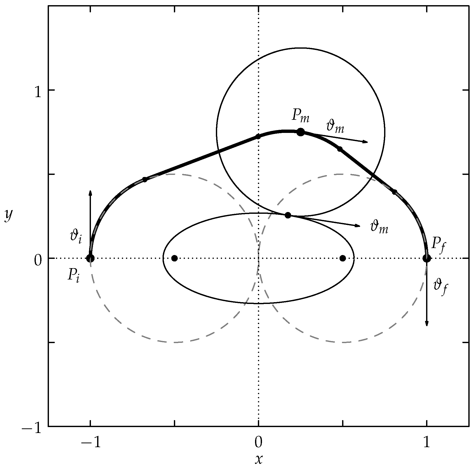
The 3PDP is formulated as follows (see Figure 1 as a reference): given an initial point $P_i=(x_i,y_i)$ with orientation ${\vartheta }_i$ and a middle point $P_m=(x_m,y_m)$ and a final point $P_f=(x_f,y_f)$ with orientation ${\vartheta }_f$, find the shortest path that begins in $P_i$ with a heading angle ${\vartheta }_i$, passes through $P_m$, and reaches $P_f$ with angle ${\vartheta }_f$; the path should not exceed a maximum absolute curvature value of $\kappa >0$ and should exhibit $G^1$ continuity.

By Bellman’s optimality principle, it is clear that the last part of the path, from $P_m$ to $P_f$, should also be the shortest path. If the angle ${\vartheta }_m$ at $P_m$ was known, this subproblem would be precisely a standard Dubins problem [21,22,23,24]. The same holds for the first path from $P_i$ to $P_f$. Thus the problem is one-dimensional since the angle ${\vartheta }_m$ at $P_m$ is the only unknown. Once ${\vartheta }_m$ is determined, the solution becomes trivial since it is just twice the application of the standard Dubins problem, as noted in [19], and it is therefore made of $3+3$ arcs of the usual Dubins type, i.e., C for circle arcs and S for straight lines. The C-type arcs are further specialized to L (left) and R (right) turns.

Moreover, the authors in [19] proved that the general solution indeed only has five arcs, with the third and fourth arcs given by circular arcs with the same orientation; e.g., the solution depicted in Figure 1 is LRL-LRL, which becomes LRLRL, representing the central arcs merged into a single L arc.

The total number of possible cases is thus in principle $6\times 6=36$ (with 6 being the number of cases of a standard point to the point Dubins problem), but we will see that only 18 are optimal and need to be considered, as listed in

Table 1. Types of the 18 admissible paths according to [19].

CCCCC:	RLRLR, LRLRL
CCCSC:	RLRSR, RLRSL, LRLSL, LRLSR
CSCCC:	RSRLR, LSRLR, RSLRL, LSLRL
CSCSC:	RSRSR, LSRSR, RSRSL, LSRSL,
	LSLSL, RSLSL, LSLSR, RSLSR

.

2.2. State of the Art

Following the discussion presented earlier, one of the most straightforward techniques for solving the Three-Point Dubins Problem (3PDP) involves discretizing the domain $[0,2\pi )$, which encompasses all possible values of the intermediate unknown angle ${\vartheta }_m$. This method evaluates the length of each resulting path configuration by systematically testing the discretized samples and then selecting the candidate with the shortest length as the optimal solution. Known as the Discretization-based method (DBM), this approach is conceptually simple and easy to implement. In practice, the interval is often sampled using 360 evenly spaced angles, a choice that offers a reasonable trade-off between resolution and computational cost. Due to its simplicity and reproducibility, the DBM is widely adopted as a benchmark reference in comparative studies assessing the efficiency and accuracy of more sophisticated solution strategies (see, for instance, [4,18,19,20]).

Despite its practical utility, the DBM is not computationally efficient in terms of accuracy. This situation arises in hierarchical motion planning frameworks, such as the Dubins Traveling Salesman Problem (DTSP), where the 3PDP serves as a core subroutine. In such contexts, the overall performance of the higher-level algorithm is directly impacted by the efficiency of the lower-level 3PDP solver. Therefore, the need for faster and more accurate alternatives has driven significant research attention toward the development of improved methodologies.

In recent years, the 3PDP has emerged as a topic of study, with multiple researchers exploring innovative formulations and computational techniques. One of the first alternatives to the DBM is developed in the mathematical framework of Inversive Geometry (IG). This approach, introduced in [18], leverages geometric transformations to derive an iterative algorithm. The core idea is to reformulate the 3PDP as a nonlinear system consisting of three equations in three unknown variables. Solving this system yields the intermediate angle ${\vartheta }_m$ more accurately and with significantly reduced computational effort compared to the DBM. However, a notable shortcoming of this method is its limited applicability: it only accommodates 8 out of the 18 theoretical path types, specifically excluding those that contain CCC (circle-circle-circle) subpaths. As a result, while IG offers an elegant and computationally appealing solution, its restricted domain of applicability reduces its general utility.

A fundamentally different strategy was proposed in [19], which introduced the polynomial-based method (PBM). This method begins with the observation that the intermediate angle ${\vartheta }_m$ satisfies a particular trigonometric relationship that can be transformed into a polynomial equation in the variable $z=tan({\vartheta }_m/2)$. For each of the 18 possible 3PDP cases, this formulation yields a single univariate polynomial. The primary strength of the PBM lies in its reduction in the geometric path planning problem to a purely algebraic one, which can be tackled using well-established polynomial root-finding techniques. Nonetheless, the method requires the generation and solutions of 18 distinct polynomial equations, each corresponding to a different path type. These polynomials vary in degree, ranging from 4 to as high as 20, and collectively may present up to 180 real or complex roots. Specifically, there are 2 polynomials of degree 4, 2 of degree 6, 10 of degree 8, and 4 of degree 20 [19].

The process of constructing these polynomials (sometimes of high degrees) introduces numerical challenges. The coefficients are derived using a repeated squaring technique intended to eliminate square roots from the expressions. This results in coefficients composed of a large number of high-degree monomials, whose values are computed using floating-point arithmetic. The approximate nature of this computation leads to numerical instability, especially for the highest-degree polynomials. Additionally, each root must be substituted back into the corresponding path model to evaluate the associated path length. Among these, the solution that results in the shortest valid path is designated as the global optimum. Despite its complexity, the PBM exhibits notable advantages over both the DBM and the IG method, particularly in terms of precision and overall computational speed.

Another recent advancement is the geometry-based method (GBM), developed in [4], which employs principles of analytic geometry to solve the 3PDP. The method is founded on a geometric insight: for the optimal path, there exists an ellipse whose foci are located at the centers of the initial and final turning circles. This ellipse is tangent to the circle centered at the intermediate point $P_m$. The angle ${\vartheta }_m$ corresponding to the optimal path is determined by the orientation of the common tangent line between this ellipse and the circle centered at $P_m$ (see Figure 2). All mentioned circles have a radius equal to the turning radius $\rho =1/\kappa$, with $\kappa$ representing the maximum allowed curvature.

This geometric construction allows the problem to be addressed analytically, offering high precision without resorting to discretization or high-degree polynomial manipulation. However, much like the IG approach, the GBM addresses only a subset of path configurations—specifically, those that do not involve CCC subpaths.

Finally, a novel solution approach, introduced in [20], applies techniques from non-smooth numerical optimization to the 3PDP. One of the central challenges in optimizing the 3PDP is the inherent discontinuity of the path length function with respect to ${\vartheta }_m$, particularly at points where the path type changes. This method directly addresses that issue by developing analytical expressions for the derivatives of the Dubins path length with respect to the optimization variable. By incorporating derivative information, the method achieves improved convergence behavior, accuracy, and runtime performance, and it is applicable across the full range of 3PDP configurations.

The present work wants to explore the possibility of using the promising machine learning-based results of our previous work [17] on the classic Dubins problem to the 3PDP. The main problem that prevents the direct use of machine learning techniques is the complexity, size, and variability of the learning space (in particular, those of the input variables). The next sections show how it is possible to reduce this complexity by leveraging the symmetries of the problem.

3. Symmetries of the Problem

This section is devoted to the study of the symmetries of the problem, which are used to reduce the complexity of the dataset required to learn the solution space.

3.1. Symmetries of the Markov–Dubins Problem

In this section, it is more convenient to consider the orientation of the curve in terms of tangent and normal vectors, $\mathit{t}$ and $\mathit{n}$, rather than using the corresponding angle $\vartheta$. The classic Dubins problem is studied, and the results are then applied to the 3PDP.

Lemma 1

(Invariance to similarity transformations). A Dubins curve is invariant to rotations, translations, and scaling.

Proof. 

The invariance to rotations and translations follows from the fundamental theorem of curves, which says that for a differentiable function $\kappa \left(s\right)\ne 0$, there exists a regular parameterized curve with curvature $\kappa \left(s\right)$ and arc-length parameterization s. Any other curve satisfying the same definition will differ by a rigid motion, i.e., a rotation or a translation (see e.g., [25]). When $\kappa \left(s\right)\equiv 0$, the curve is a straight line, which is again unique up to rigid motions. If the curvature is zero at a single point, the tangent is still well-defined, and there will be an inflection point, at which the normal vector changes direction.

To show invariance to scaling, suppose that C is a Dubins curve: since it is a juxtaposition of at most three circular or line arcs of a specified length, it is possible to show the scaling property for each subarc. Hence, we assume that C is either an arc or a line segment of length ℓ and curvature parameter $\kappa$ that interpolates an initial point and a final point, $P_i=C\left(0\right)$ and $P_f=C(\ell )$, respectively. The constant parameter $\kappa$ models the curvature of the circle (if different from zero) and that of a line segment if it is identically equal to zero. We will show that the curve $C_{\lambda }$ with parameter ${\kappa }_{\lambda }$, which interpolates $\lambda P_i$ and $\lambda P_f$, for $\lambda >0$ is the curve C multiplied by $\lambda$; that is, $C_{\lambda }\left(s\right)=\lambda C\left(s\right)$. This accounts for finding the new parameter ${\kappa }_{\lambda }$ that satisfies the interpolation conditions of $C_{\lambda }\left(0\right)=\lambda P_i$ and $C_{\lambda }(\lambda \ell )=\lambda P_f$.

We claim that ${\kappa }_{\lambda }=\kappa /\lambda$ and use the fundamental theorem of curves. The Frenet–Serret equations for the tangent vector ${\mathit{t}}_{\lambda }$ and the normal vector ${\mathit{n}}_{\lambda }$ for $C_{\lambda }$ are

$$\begin{array}{ccc}\hfill {\displaystyle \frac{\mathrm{d}{\mathit{t}}_{\lambda }\left(u\right)}{\mathrm{d}u}}& =& {\displaystyle \frac{\kappa }{\lambda }}{\mathit{n}}_{\lambda }\left(u\right)\hfill \\ \hfill {\displaystyle \frac{\mathrm{d}{\mathit{n}}_{\lambda }\left(u\right)}{\mathrm{d}u}}& =& -{\displaystyle \frac{\kappa }{\lambda }}{\mathit{t}}_{\lambda }\left(u\right).\hfill \end{array}$$

Now, with the change in variable $v=u/\lambda$, which implies the differential $\mathrm{d}v=\mathrm{d}u/\lambda$, the previous equations become

$$\begin{array}{ccccccc}\hfill {\displaystyle \frac{\mathrm{d}{\mathit{t}}_{\lambda }\left(u\right)}{\mathrm{d}u}}& =& {\displaystyle \frac{\mathrm{d}{\mathit{t}}_{\lambda }}{\mathrm{d}v}}{\displaystyle \frac{\mathrm{d}v}{\mathrm{d}u}}={\displaystyle \frac{1}{\lambda }}{\displaystyle \frac{\mathrm{d}{\mathit{t}}_{\lambda }\left(v\right)}{\mathrm{d}v}}={\displaystyle \frac{\kappa }{\lambda }}{\mathit{n}}_{\lambda }\left(v\right)\hfill & \Rightarrow & \hfill {\displaystyle \frac{\mathrm{d}{\mathit{t}}_{\lambda }\left(v\right)}{\mathrm{d}v}}& =& \kappa {\mathit{n}}_{\lambda }\left(v\right)\hfill \\ \hfill {\displaystyle \frac{\mathrm{d}{\mathit{n}}_{\lambda }\left(u\right)}{\mathrm{d}u}}& =& {\displaystyle \frac{\mathrm{d}{\mathit{n}}_{\lambda }}{\mathrm{d}v}}{\displaystyle \frac{\mathrm{d}v}{\mathrm{d}u}}={\displaystyle \frac{1}{\lambda }}{\displaystyle \frac{\mathrm{d}{\mathit{n}}_{\lambda }\left(v\right)}{\mathrm{d}v}}=-{\displaystyle \frac{\kappa }{\lambda }}{\mathit{t}}_{\lambda }\left(v\right)\hfill & \Rightarrow & \hfill {\displaystyle \frac{\mathrm{d}{\mathit{n}}_{\lambda }\left(v\right)}{\mathrm{d}v}}& =& -\kappa {\mathit{t}}_{\lambda }\left(v\right).\hfill \end{array}$$

This is true because the Frenet–Serret equations hold for every parameterization. The integration of the equations goes as follows: to obtain $C_{\lambda }$, we need to integrate its tangent vector; hence,

$$\begin{array}{ccc}\hfill {\mathit{t}}_{\lambda }\left(s\right)& =& {\mathit{t}}_0+{\int }_0^{\lambda s}{\displaystyle \frac{\mathrm{d}{\mathit{t}}_{\lambda }\left(u\right)}{\mathrm{d}u}}\mathrm{d}u={\mathit{t}}_0+{\int }_0^s{\displaystyle \frac{1}{\lambda }}{\displaystyle \frac{\mathrm{d}{\mathit{t}}_{\lambda }\left(v\right)}{\mathrm{d}v}}·\lambda \mathrm{d}v=\mathit{t}\left(s\right),\hfill \\ \hfill C_{\lambda }\left(s\right)& =& \lambda P_i+{\int }_0^{\lambda s}\left({\mathit{t}}_0+{\int }_0^{t/\lambda }{\displaystyle \frac{1}{\lambda }}{\displaystyle \frac{\mathrm{d}{\mathit{t}}_{\lambda }\left(v\right)}{\mathrm{d}v}}·\lambda \mathrm{d}v\right)\mathrm{d}t\hfill \\ \hfill & =& \lambda P_i+{\int }_0^s\left({\mathit{t}}_0+{\int }_0^{\widehat{s}}{\displaystyle \frac{\mathrm{d}{\mathit{t}}_{\lambda }\left(v\right)}{\mathrm{d}v}}\mathrm{d}v\right)\lambda \mathrm{d}\widehat{s}\hfill \\ \hfill & =& \lambda \mathrm{(}{P}_i+{\int }_0^s\mathit{t}\left(\widehat{s}\right)\mathrm{d}\widehat{s}\mathrm{)}\hfill \\ \hfill & =& \lambda C\left(s\right),\hfill \end{array}$$

which holds for all $s\in [0,\ell ]$. □

Lemma 2

(Symmetry). A Dubins curve is symmetric; that is, the curve $C\left(s\right)$ that interpolates $(P_i,{\mathit{t}}_i)$ and $(P_f,{\mathit{t}}_f)$ with curvature κ and length ℓ has the same trace as the Dubins curve $C_{\mathit{sym}}\left(s\right)$ that interpolates a starting pose $(P_f,-{\mathit{t}}_f)$, a final pose $(P_i,-{\mathit{t}}_i)$, and $C_{\mathit{sym}}(\ell -s)=C\left(s\right)$ with tangent ${\mathit{t}}_{\mathit{sym}}(\ell -s)=-\mathit{t}\left(s\right)$.

Proof. 

We have that

$$\begin{array}{ccc}\hfill {\mathit{t}}_{\mathrm{sym}}(\ell -s)& =& -{\mathit{t}}_f+{\int }_0^{\ell -s}{\displaystyle \frac{\mathrm{d}{\mathit{t}}_{\mathrm{sym}}\left(u\right)}{\mathrm{d}u}}\mathrm{d}u\hfill \\ \hfill & =& -{\mathit{t}}_f+{\int }_{\ell }^s{\displaystyle \frac{\mathrm{d}{\mathit{t}}_{\mathrm{sym}}\left(v\right)}{\mathrm{d}v}}\mathrm{d}v\hfill \\ \hfill & =& -{\mathit{t}}_f-{\int }_s^{\ell }{\displaystyle \frac{\mathrm{d}{\mathit{t}}_{\mathrm{sym}}\left(v\right)}{\mathrm{d}v}}\mathrm{d}v\hfill \\ \hfill & =& -{\mathit{t}}_f+{\int }_s^{\ell }{\displaystyle \frac{\mathrm{d}\mathit{t}\left(v\right)}{\mathrm{d}v}}\mathrm{d}v\hfill \\ \hfill & =& -\left({\mathit{t}}_i+{\int }_0^{\ell }{\displaystyle \frac{\mathrm{d}\mathit{t}\left(v\right)}{\mathrm{d}v}}\mathrm{d}v\right)+{\int }_s^{\ell }{\displaystyle \frac{\mathrm{d}\mathit{t}\left(v\right)}{\mathrm{d}v}}\mathrm{d}v\hfill \\ \hfill & =& -{\mathit{t}}_i-{\int }_0^s{\displaystyle \frac{\mathrm{d}\mathit{t}\left(v\right)}{\mathrm{d}v}}\mathrm{d}v\hfill \\ \hfill & =& -\mathit{t}\left(s\right).\hfill \end{array}$$

Regarding the curves C and $C_{\mathrm{sym}}$,

$$\begin{array}{ccc}\hfill C_{\mathrm{sym}}(\ell -s)& =& P_f+{\int }_0^{\ell -s}\left(-{\mathit{t}}_f+{\int }_0^{\widehat{s}}{\displaystyle \frac{\mathrm{d}{\mathit{t}}_{\mathrm{sym}}\left(u\right)}{\mathrm{d}u}}\mathrm{d}u\right)\mathrm{d}\widehat{s}\mathrm{with}[v=\ell -u]\hfill \\ \hfill & =& P_f+{\int }_0^{\ell -s}\left(-{\mathit{t}}_f+{\int }_{\ell }^{\ell -\widehat{s}}{\displaystyle \frac{\mathrm{d}{\mathit{t}}_{\mathrm{sym}}\left(v\right)}{\mathrm{d}v}}\mathrm{d}v\right)\mathrm{d}\widehat{s}\hfill \\ \hfill & =& P_f+{\int }_0^{\ell -s}\left(-{\mathit{t}}_f+{\int }_{\ell -\widehat{s}}^{\ell }{\displaystyle \frac{\mathrm{d}\mathit{t}\left(v\right)}{\mathrm{d}v}}\mathrm{d}v\right)\mathrm{d}\widehat{s}\mathrm{with}[t=\ell -\widehat{s}]\hfill \\ \hfill & =& P_f-{\int }_{\ell }^s\left(-{\mathit{t}}_f+{\int }_t^{\ell }{\displaystyle \frac{\mathrm{d}\mathit{t}\left(v\right)}{\mathrm{d}v}}\mathrm{d}v\right)\mathrm{d}t\hfill \\ \hfill & =& P_f-{\int }_{\ell }^s\left(-{\mathit{t}}_i-{\int }_0^{\ell }{\displaystyle \frac{\mathrm{d}\mathit{t}\left(v\right)}{\mathrm{d}v}}\mathrm{d}v+{\int }_t^{\ell }{\displaystyle \frac{\mathrm{d}\mathit{t}\left(v\right)}{\mathrm{d}v}}\mathrm{d}v\right)\mathrm{d}t\hfill \\ \hfill & =& P_i+{\int }_0^s\left({\mathit{t}}_i+{\int }_0^t{\displaystyle \frac{\mathrm{d}\mathit{t}\left(v\right)}{\mathrm{d}v}}\mathrm{d}v\right)\mathrm{d}t\hfill \\ \hfill & =& C\left(s\right),\hfill \end{array}$$

where the last step involves writing $P_f$ in integral form. □

The next section takes advantage of these two lemmas to transform a 3PDP path and reduce the input space for the machine learning phase. The 3PDP has nine input parameters, namely the six spatial coordinates of $P_i$, $P_m$, $P_f$, two angles (${\vartheta }_i$ and ${\vartheta }_f$), and the minimum turning radius $\rho$ (or, equivalently, the maximum curvature $\kappa$). The solution space is one-dimensional in terms of either the intermediate angle ${\vartheta }_m$ at $P_m$ or the equivalent maneuver-type sequence (see Table 1).

3.2. Symmetries of the 3PDP

The 3PDP is just the juxtaposition of two Dubins paths; hence, the 3PDP solution inherits the symmetry properties discussed in the previous section. We will use them in the next section to reduce the complexity of the input parameters space. In this section, we specialize the previous lemmas to reflect symmetries around the horizontal and vertical axes. Also, instead of the tangent vectors ${\mathit{t}}_i$, ${\mathit{t}}_f$, etc., we use their corresponding angles ${\vartheta }_i$, ${\vartheta }_f$, etc.; e.g., ${\mathit{t}}_i=(cos\left({\vartheta }_i\right),sin\left({\vartheta }_i\right))$.

Lemma 3

(Horizontal reflection). Consider the 3PDP defined as $P_i$, ${\vartheta }_i$, $P_f$, and ${\vartheta }_f$ passing through $P_m=(x_m,y_m)$, with $y_m<0$ and the optimal angle ${\vartheta }_m$. The $x-$axis-reflected problem has the same $P_i$ and $P_f$, with $P_m^h=(x_m,-y_m)$, initial angle ${\vartheta }_i^h=-{\vartheta }_i$, final angle ${\vartheta }_f^h=-{\vartheta }_f$, and ${\vartheta }_m^h=2\pi -{\vartheta }_m$.

Proof. 

The lemma follows from Lemma 2 applied to each of the two subDubins paths. □

We can also assume that $x_m\ge 0$ thanks to the following lemma.

Lemma 4

(Vertical reflection). Consider the 3PDP defined as $P_i$, ${\vartheta }_i$, $P_f$, and ${\vartheta }_f$ passing through $P_m=(x_m,y_m)$, with $x_m<0$ and the optimal angle ${\vartheta }_m$. The $y-$axis-reflected problem has the same $P_i$ and $P_f$, with $P_m^v=(-x_m,y_m)$, initial angle ${\vartheta }_i^v=-{\vartheta }_f$, final angle ${\vartheta }_f^v=-{\vartheta }_i$, and ${\vartheta }_m^v=2\pi -{\vartheta }_m$.

Proof. 

The lemma follows from Lemma 2 applied to each of the two subDubins paths. □

4. Construction of the Training Set

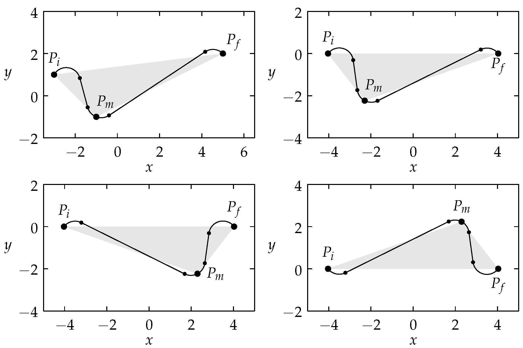
The 3PDP has nine input variables: Six are given by the spatial information of the three waypoints. Two correspond to the initial and final angles, and one is for the maximum curvature (Figure 3 top left). The solution is characterized by the intermediate angle ${\vartheta }_m$ and by the corresponding maneuver from the list of Table 1. We propose a method to reduce the number of variables to six; moreover, with the presented transformation, the spatial variables do not span $\mathbb{R}$ anymore, but they are constrained in a compact set, where we can efficiently collect meaningful samples to build a dataset to be learned with ML techniques.

Consider the original data of the problem, that is, generic points $P_i$, $P_m$, and $P_f$ in the plane with the initial and final angles ${\vartheta }_i$ and ${\vartheta }_f$, respectively. Suppose that ${\vartheta }_m$ is the angle at $P_m$, which is the solution of the 3PDP. Let $d=\left|\right|P_i-P_f\left|\right|$ be the distance of the initial and final points. Without loss of generality, thanks to the previous lemmas, it is possible to

1.

Translate and rotate the points such that $P_i\mapsto (-c,0)$ and $P_f\mapsto (c,0)$, where $c=d/2$ (Figure 3 top right). This is conducted with the invertible map T, where

$$\begin{gathered} T\left(\left[\begin{array}{c}x\\ y\end{array}\right]\right)=\left[\begin{array}{cc}cos\varphi & -sin\varphi \\ sin\varphi & cos\varphi \end{array}\right]\left(\left[\begin{array}{c}x\\ y\end{array}\right]-\overline{P}\right)-\left[\begin{array}{c}-c\\ 0\end{array}\right],\mathrm{with} \\ \varphi =-\mathrm{atan}2(y_f-y_i,x_f-x_i),\overline{P}={\displaystyle \frac{P_i+P_f}{2}}. \end{gathered}$$

The new angle ${\vartheta }_m^{\left(1\right)}$ produced by this first step, which is a solution of this rotated and shifted problem, relates to the original angle ${\vartheta }_m$ by means of ${\vartheta }_m^{\left(1\right)}={\vartheta }_m+\varphi$.

2.

After this step, $x_m$ can be negative; i.e., $P_m$ is to the left of the y-axis. We reflect the problem with respect to the vertical axis so that the new $P_m$ has $x_m\ge 0$ (Figure 3 bottom left). The angle produced by this second step is ${\vartheta }_m^{\left(2\right)}=2\pi -{\vartheta }_m^{\left(1\right)}$.

3.

At this point, $y_m$ can be negative; i.e., $P_m$ is under the x-axis. We can reflect the problem with respect to the horizontal axis so that the new $P_m$ has $y_m\ge 0$ (Figure 3 bottom right). The angle produced by this third step is ${\vartheta }_m^{\left(3\right)}=2\pi -{\vartheta }_m^{\left(2\right)}$.

4.

The problem can be further standardized by scaling the three points by a factor of $r=max(c,x_m,y_m)$. This step produces a triangle with a base from $(-c,0)$ to $(c,0)$ for $c\in [0,1]$; the point $P_m$ is mapped to the unitary square $P_m\in [0,1]\times [0,1]$. Depending on which of the three variables realizes the maximum in r, one or more of the variables $c,x_m,y_m$ will be one. This corresponds to four cases when the triangle is acute or obtuse with $P_m$ “far” or “close”, specifically

(a)

if $x_m\le c$ and $y_m\le c$, the point $P_m$ is contained inside the unitary square and $c=1$;

(b)

if $x_m\le c$ and $y_m>c$, then $y_m=1$;

(c)

if $x_m>c$ and $y_m\le c$, then $c<1$ and $x_m=1$;

(d)

if $x_m>c$ and $y_m>c$, then $c<1$ and the maximum between the components of $P_m$ will be unitary.

Since this scaling operation is the same on both axes, the solution angle is not altered by this step.

These four steps allow us to construct a comprehensive dataset of test cases that virtually sample the whole input space of the problem, without loss of generality. The input parameters have been reduced from 9 to 6, namely

$$P_i=(-c,0),P_m=(x_m,y_m),P_f=(c,0),{\vartheta }_i,{\vartheta }_f,\kappa ,$$

with the variables to be sampled in the following ranges:

$$c\in [0,1],(x_m,y_m)\in [0,1]\times [0,1],{\vartheta }_i,{\vartheta }_f\in [0,2\pi ),\kappa \in (0,\infty ).$$

Remark 1.

We underline that with this choice it is possible to capture all possible positions on different scales. The variables c and $P_m$ and the angles are confined in bounded sets that can be sampled in a meaningful way; only the maximum curvature can be arbitrarily large. However, as we have previously remarked, e.g., [17,24], for large values of κ (large can be considered $\kappa >6$; see [17]), the solution curve does not change very much. The intuition behind this fact is that the higher the curvature, the better the steering capability of the vehicle, which, at the limit $\kappa \to \infty$, can rotate on the spot, making the path tend to a polyline (a 3PDP path of type CSCSC) with arbitrary small rounded corners. That is, the C arcs tend to zero, and the line segments S tend to the distances $\left|\right|P_i-P_m\left|\right|$ and $\left|\right|P_f-P_m\left|\right|$, respectively.

The overall result of this transformation is two-fold: first, we have reduced the complexity from 9 variables to 6 variables; second, these 6 variables can be sampled in a small bounded region, and the spatial coordinates of the points do not range in the whole ${\mathbb{R}}^2$ plane anymore.

To construct the dataset, we discretized the parameters as follows: a step size of $0.1$ for c, $x_m$, and $y_m$; a step size of $\pi /24$ for ${\vartheta }_i$ and ${\vartheta }_f$ within the interval $[-\pi ,\pi )$; and a step size of $0.2$ for $\kappa \in [0.2,6]$. This procedure yielded approximately $2.3\times {10}^7$ candidate instances. We subsequently removed configurations, such as cases where $P_m=P_i$ or $P_m=P_f$, resulting in a final dataset comprising 17,932,148 valid cases. For each instance, we recorded the optimal maneuver and the corresponding optimal angle identified through the iterative dynamic programming approach (https://www.github.com/icosac/mpdp, accessed on 10 December 2025) employed in [2].

5. Training Phase

There are many ML techniques available: for our purposes, we needed to find a trade-off between effective learning capability and speed of inference, which has to be small compared with the time required to enumerate the 18 cases. Therefore, we found out that the two following networks, one for regressing the angle ${\vartheta }_m$ and one for predicting the case label, being relatively simple, show a good trade-off between the two requirements. We conducted a test campaign with different hyperparameters and structures, converging to the presented case.

We tested two different models, a regression one and a classification one, to showcase two possible learning approaches.

• The regression models for finding the first estimate of the optimal angle for the problem subsequently use the iterative algorithm [2] to either improve on the solution, leading to a better approximation of the optimal angle with fewer iterations, or improve the accuracy score for the same number of iterations.
• The classification model allows for identifying the type of maneuver and then computing the optimal angle ${\vartheta }_m$ by solving the corresponding polynomial formula, as shown in [19] for the PBM.

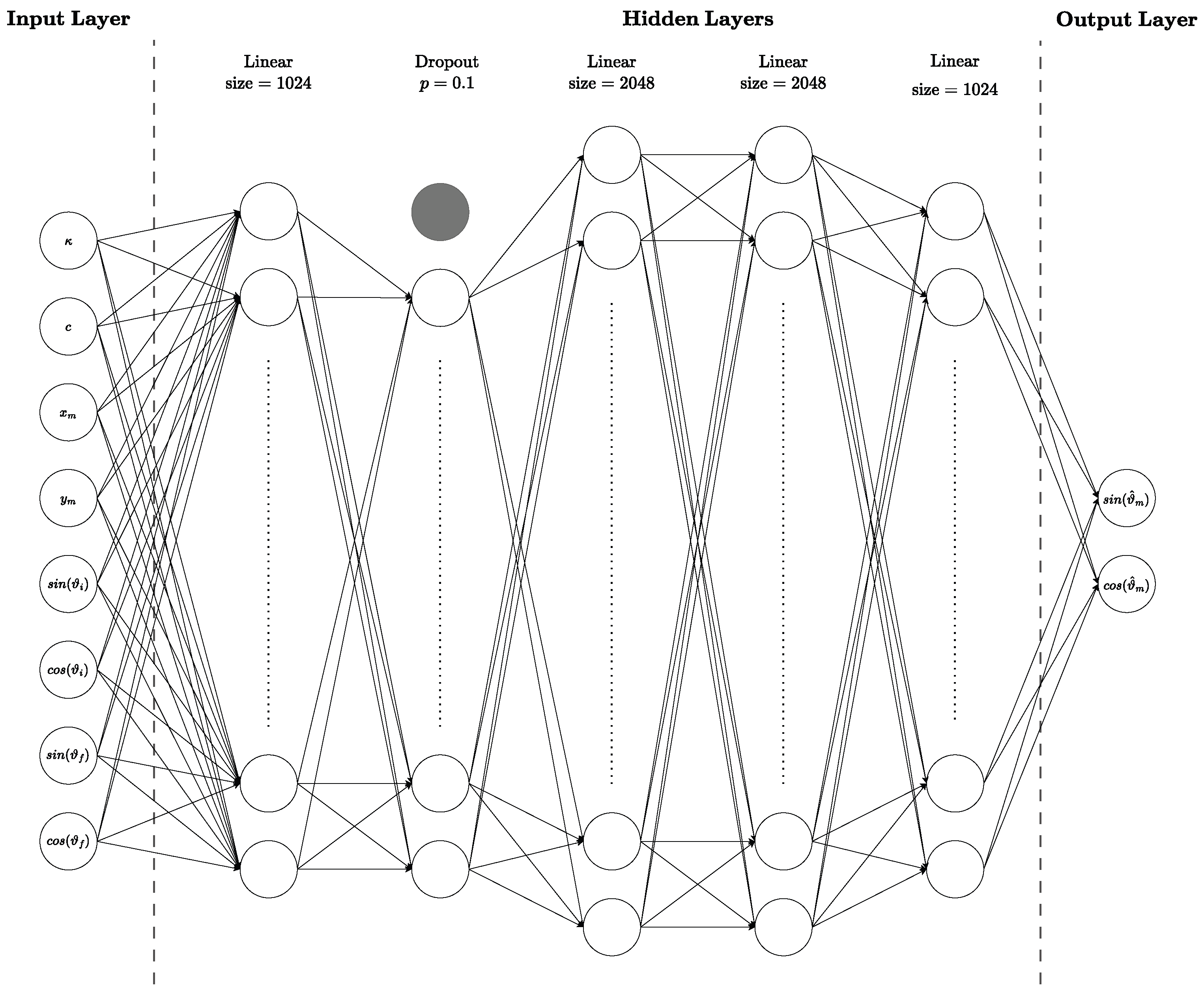
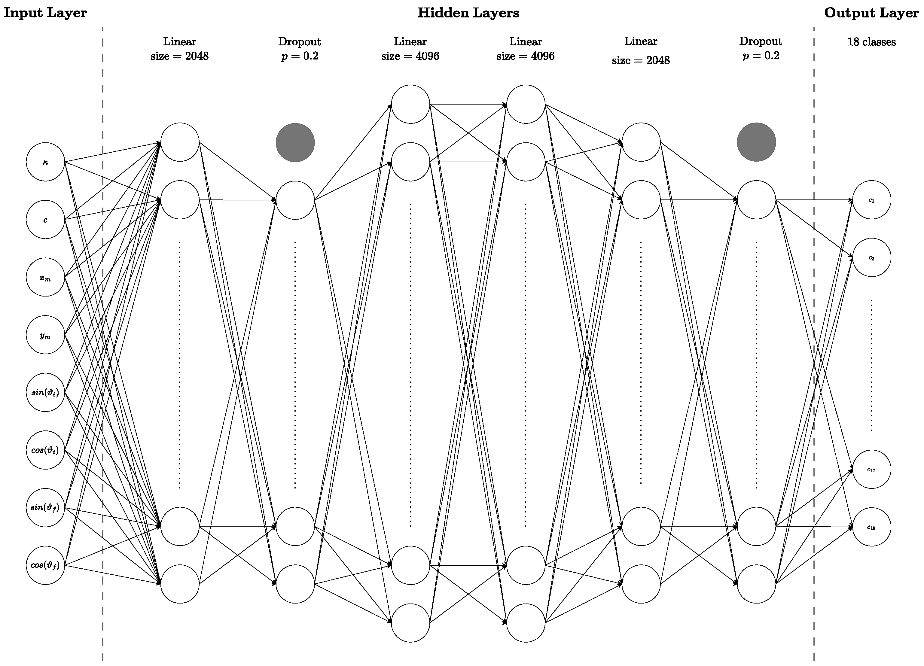
The regression and classification networks consist of three and four layers, respectively, and their architectures are illustrated in Figure 4 and Figure 5, respectively. To improve generalization and mitigate overfitting arising from structured patterns in the dataset, dropout layers were incorporated into both models [26]. Moreover, the two architectures differ in their choice of activation functions: while the classification network employs standard nonlinearities, the regression network adopts the leaky ReLU activation function, which consistently yielded superior predictive performance compared to the standard ReLU by mitigating the issue of inactive neurons [27,28].

Each dataset entry is originally described by six parameters: $\kappa ,c,x_m,y_m,{\vartheta }_i,{\vartheta }_f$. However, to address the symmetries introduced by the angular features and to improve the representational capacity of the network, we reformulated the inputs into eight features: $\kappa ,c,x_m,y_m,sin\left({\vartheta }_i\right),cos\left({\vartheta }_i\right),sin\left({\vartheta }_f\right),cos\left({\vartheta }_f\right)$. The regression model the sine and cosine of the predicted angle as output, ensuring a continuous and numerically stable representation of angular values. The classification model outputs a probability distribution over the maneuver classes, which are obtained via a softmax layer, which maps each maneuver label to its associated probability. The probability and the corresponding maneuver are presented and sorted in decreasing order; i.e., the most likely case comes first.

For training, the classification model employed a cross-entropy loss, while the regression model used a mean squared error loss. Both models used the Adam optimizer. In both cases, we set the learning rate to $1\times {10}^{-5}$, the weight decay to $1\times {10}^{-5}$, and the batch size to 64. To ensure repeatability, the random seed was fixed to 42 across training and experiments. The choice of these hyperparameters was made after preliminary experiments aimed at identifying effective configurations.

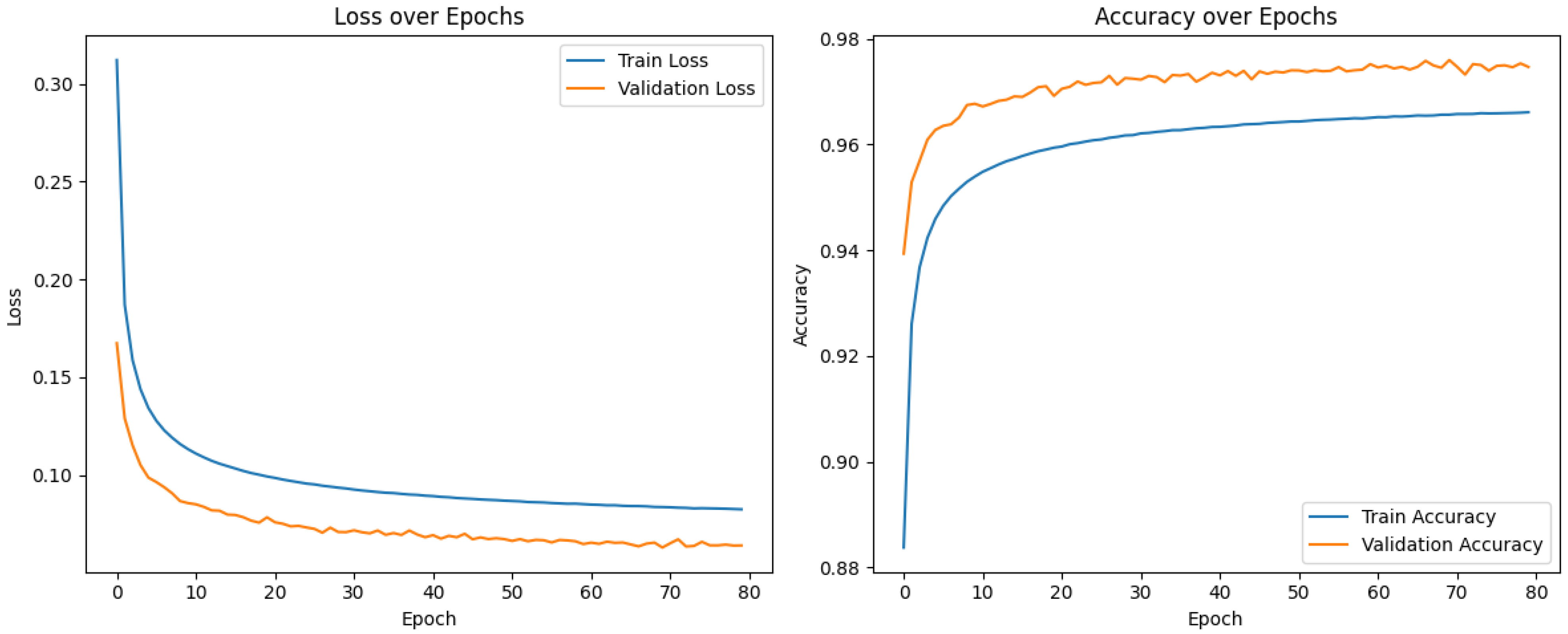
Both models were trained on the dataset described in Section 4, which was partitioned into 70% for training, 15% for validation, and 15% for testing. Training was performed on a cluster equipped with NVIDIA A100 GPUs (80 GB of VRAM), with a single GPU allocated per each run. Each model was trained for a maximum of 150 epochs with early stopping (patience = 10 epochs). The regression model converged after 111 epochs, requiring approximately $22,363$ s (about 6 h), while the classification model converged after 88 epochs, with a total training time of approximately 60,793 s (about 17 h). The loss curves across epochs are reported in Figure 6.

The dataset and the trained models are available online [29], while the code is available at (https://www.github.com/icosac/mpdp, accessed on 10 December 2025).

6. Results

6.1. Classification Results on the Test Set

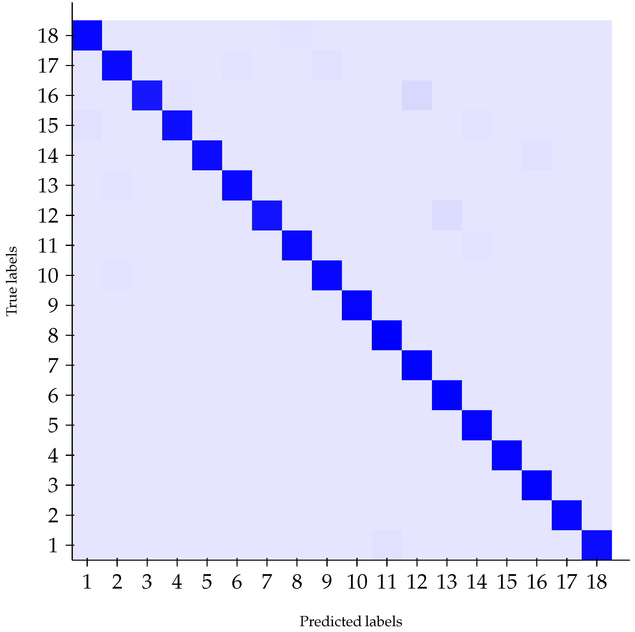
The classification model achieved a test loss of $0.0644$ and a top-1 accuracy of $97.5\%$ on the test set. Accuracy increased rapidly with higher ranks, exceeding $99.99\%$ in top-4 predictions and reaching $100\%$ from top-5 onwards. Here, top-k accuracy denotes the proportion of test instances for which the correct label is contained among the k predicted classes with the highest probabilities. The detailed classification report is shown above, with precision, recall, and F1-scores consistently above $0.95$ across all maneuver classes. The confusion matrix for the top-1 results (Figure 7) shows strong diagonal dominance, indicating that the vast majority of samples are correctly classified. Classes with a larger number of instances, such as labels 10–13, exhibit near-perfect recall, with very few misclassifications. The model demonstrates slightly lower performance on classes with fewer samples (e.g., classes 2, 3, 6, and 15), where a modest increase in confusion with neighboring classes can be observed. The errors that do occur tend to involve confusion between classes corresponding to maneuvers with similar geometric characteristics. For example, class 2 is sometimes misclassified as class 7 or 8, and class 15 is occasionally confused with class 16, reflecting structural similarities in their maneuver patterns. Despite these localized errors, precision and recall remain consistently above $0.90$ for all classes, confirming that the classifier generalizes well across both frequent and less frequent maneuver types. Overall, the confusion matrix confirms the robustness of the classification network, with most of the residual error attributable to inherently ambiguous cases rather than systematic model bias. Results are summarized in

Table 2. Table summarizing the results obtained in Section 6.1 and Section 6.2.

Method	Test Loss	MSE		Mean Angular	Accuracy (%)			F1-Score
		Sine	Cosine	Error (Rad)	Top-1	Top-4	Top-5
Classification	0.0644	-	-	-	97.54	99.99	100.0	0.95
Regression	0.0093	0.0106	0.0079	0.0467	-	-	-	-

.

6.2. Regression Results on the Test Set

On the test set, the regression model achieved the following performance: a test loss of $0.0093$; mean squared error (MSE) values of $0.0106$ and $0.0079$ for the sine and cosine components, respectively; mean absolute error (MAE) values of $0.0351$ (sine) and $0.0328$ (cosine); and $R^2$ scores of $0.9746$ (sine) and $0.9819$ (cosine). The model yielded a mean angular error of $0.0467$ radians ($2.{68}^{°}$) and a median angular error of $0.0160$ radians ($0.{92}^{°}$). Results are summarized in Table 2.

6.3. Remarks on Performance

We evaluated the inference performance of the models using a workstation equipped with 64 GB of DDR5 RAM, an NVIDIA RTX 4070 Ti (12 GB GDDR6X), and an AMD Ryzen 7 7700X CPU. All experiments were conducted on a subset of 10,000 samples from the test sets, repeating each query 1000 times to ensure stable results.

The average inference time per query is $0.08$ ms for the regression model and $0.27$ ms for the classification model. Model loading requires, on average, $40.2$ ms and $121.7$ ms, respectively. However, we emphasize that the loading cost is paid only once: after initialization, an arbitrary number of inference queries can be processed efficiently.

When using the classification model, the network outputs a probability distribution over the IDs of the maneuver. The final solution can then be recovered by computing the corresponding polynomial using the closed-form equations provided in [19]. Computing all 18 configurations requires, on average, $21.8$ ms, whereas evaluating only the top-5 most likely cases reduces this time to $3.7$ ms. Overall, this results in a $5\times$ speed improvement over evaluating the full polynomial set while maintaining accuracy on the best predicted solutions.

With the regression model, the neural network directly predicts an initial estimate of the optimal intermediate angle. This first guess can significantly accelerate sampling-based methods. We compare the DBM planner [20] against the iterative refinement approach (IDP) [2]. In its standard configuration, the DBM samples 360 discrete angles per point, whereas IDP samples N angles and refines the solution locally M times. IDP has the same computational cost as the DBM when $N·(M+1)\approx 360$. By initializing IDP with neural prediction, we can reduce both discretization and refinement without compromising optimality.

In our experiments, the DBM required $0.85$ ms on average and achieved a mean error of $3\times {10}^{-4}$ in the optimal length. Using the regression-based initialization, IDP already converged to a better solution at $N=90, M=1$, reducing runtime to $0.48$ ms while obtaining a mean error of $1\times {10}^{-4}$. These results demonstrate a nearly $2\times$ speed improvement when using the neural initial guess. An alternative way of using our result is to consider the same computational effort, i.e., the same time as the DBM, while obtaining a more accurate solution.

Finally, we note a trade-off: while the DBM-based sampling approaches are faster than the PBMs used with the classification model, they do not guarantee convergence to the globally optimal trajectory in all cases. In contrast, the PBMs yield a more precise solution at the cost of increased computation time.

6.4. Study Case

We conclude this section with an example function to show the features and benefits of our approach. Consider the following instance of the problem:

$$\begin{array}{c}{P}_i=\left(-1,0\right),P_m=\left({\displaystyle \frac{1}{4}},{\displaystyle \frac{3}{4}}\right),P_f=\left(1,0\right),\\ {\vartheta }_i={\displaystyle \frac{\pi }{2}},\kappa =2={\displaystyle \frac{1}{\rho }},{\vartheta }_f=-{\displaystyle \frac{\pi }{2}}.\end{array}$$

(1)

It has been carefully chosen because it is a balanced example between complexity (a polynomial of the PBM of moderate degree), clarity (exact coefficients), and small numbers. A general case exhibits a much wilder behavior in the coefficients of the polynomial, as shown in [19]), and does not lend itself to a clean explanation.

The transformation to map the original data to the canonical space (see Figure 3) follows the steps of Section 4. The first one gives an angle $\varphi =0$ with $c=d=1$ (step 1). Step 2 is not necessary since $x_m\ge 0$; similarly, step 3 is not need as $y_m\ge 0$. Finally, the scaling factor is $r=max(c,x_m,y_m)=1$ (step 4). Therefore, for the present example, the original and the canonical spaces are the same. We now show how to take advantage of our results to solve an instance of the problem and compare the steps required by other methods to compute the solution, which is graphically shown in Figure 2 together with the GBM solution.

The inference phase of the specific maneuver prediction is

$$[11,18,7,9,13,12,6,3,1,16,17,2,10,15,4,5,8,14],$$

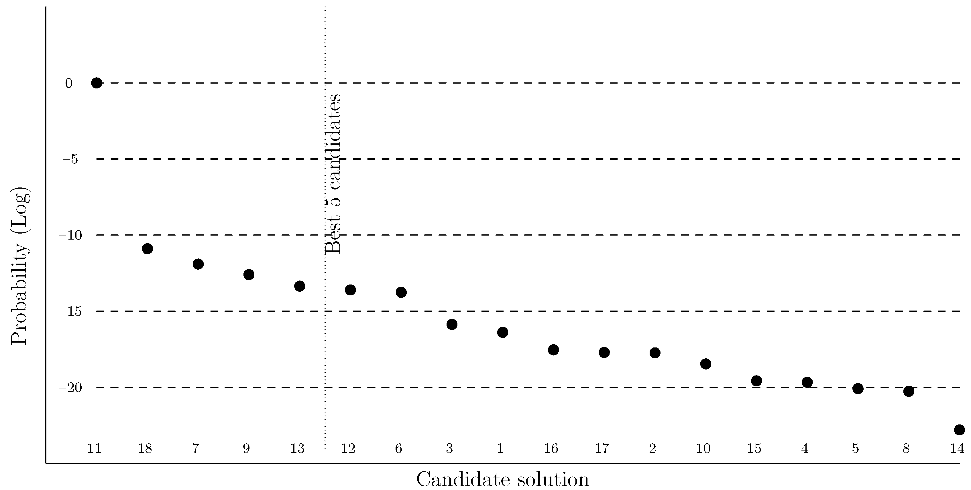
with the probability of each candidate plotted in logarithmic scale for simplicity, as shown in Figure 8. Maneuver 11, corresponding to RSRSR, turns out to be the most probable, with a probability of essentially one. Indeed, the other candidates have values decreasing from ${10}^{-11}$ to ${10}^{-24}$.

The regressed angle is

$${\widehat{\vartheta }}_m=-0.13279377\equiv 6.150391538\left(\mathrm{mod}2\pi \right).$$

Comparison with the true values. By solving the problem with a standard method, for instance the DBM, or with [19,20], we obtain that maneuver 11 yields the shortest path with the optimal angle ${\vartheta }_m=6.1314766733$ at the intermediate point $P_m$. Therefore, the predicted solution is already correct with the first candidate (with a strong probability), whereas the angular error is

$$|{\widehat{\vartheta }}_m-{\vartheta }_m|=0.018914865\left[\mathrm{rad}\right]=1.08\left[\mathrm{deg}\right],$$

meaning an error in the angle prediction of about 1 degree.

Comparison with the PBM and improvement. The PBM [19] requires us to solve for the roots of the 18 polynomials with degrees between 4 and 20 and to evaluate each candidate solution to retain the shortest one. The polynomials are expressed in the variable $z=tan({\vartheta }_m/2)$.

The contributions of our work to improve this method are two-fold: (i) we can restrict the 18 cases to 5, and (ii) we can use the regressed variable ${\widehat{\vartheta }}_m$ to either start a Newton-like method close to the correct root or select the correct roots among the others. In this example, we show both cases. Without loss of generality and for simplicity, we focus only on the first candidate solution, RSRSR (and because it is already the correct solution). However, the analysis of further candidates is analogous to what follows.

We built, following [19], the polynomial $p\left(z\right)$ corresponding to the RSRSR case with the specific values of the current example (1), which is

$$p\left(z\right)=25z^6-180z^5-85z^4+24z^3-13z^2+12z+1.$$

(2)

We can solve for all the roots of $p\left(z\right)$ simultaneously using a QR-based method (e.g., like Matlab’s “roots” command), or we can focus on a single root using a Newton-like method. By inspecting the polynomial with a computer algebra system (CAS), we can see that it can be factored into $p\left(z\right)=\left(z^2+{\displaystyle \frac{1}{5}}\right)(5z^4-36z^3-18z^2+12z+1)$: this step is not needed but is added for clarity. Solving (2) for all the roots at once, we find that $p\left(z\right)$ has four real roots, $z_1\approx -0.790$, $z_2\approx -0.07600013804$, $z_3\approx 0.436$, and $z_4\approx 7.630$, and two complex roots, $z_{5,6}=\pm i\sqrt{5}/5$, which can be neglected.

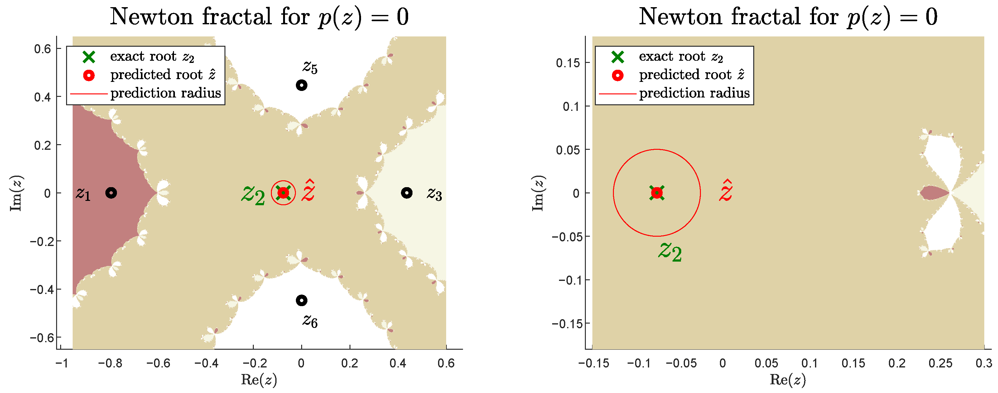
We identify root $z_2$ to be the correct one, as it is the closest to the predicted root $\widehat{z}=tan({\widehat{\vartheta }}_m/2)=-0.0664946282$. As an alternative (and faster) method, we can start a Newton method with the initial guess given by $\widehat{z}$, a value which is close to the root itself and contained in the attraction basin of $z_2$, as shown in Figure 9. In this case as well, the method converges to the same value $z_2\approx -0.07600013804$. The Newton fractal associated to $p\left(z\right)$ of Figure 9 shows that there is enough margin for the estimates of our method to remain inside the attraction basin of the correct root $z_2$, thus also reducing the need to compute all six roots of $p\left(z\right)$ and test each of them for the best path length, which further improves the overall 3PDP solution process.

Another option of using our result in a more conservative way is to compute all the roots of $p\left(z\right)$ and then test the length of the path resulting from the closest roots to $\widehat{z}$ only. In our example, we use $z_1$, $z_2$, and $z_3$. Finally, the regressed variable can be used for any other methods (e.g., IG or GBM) that look for the root by iteratively solving a nonlinear system of equations.

6.5. A Counterexample

This section is devoted to discussing what can happen in cases of multiple wrong predictions, that is, if the correct maneuver is not in the first top-5 candidates predicted with the neural network. We propose a concrete study case with the following instance of the problem:

$$\begin{array}{c}{P}_i=\left(-1,0\right),P_m=\left({\displaystyle \frac{1}{10}},{\displaystyle \frac{1}{10}}\right),P_f=\left(1,0\right),\\ {\vartheta }_i={\displaystyle \frac{5\pi }{12}},\kappa ={\displaystyle \frac{17}{10}}={\displaystyle \frac{1}{\rho }},{\vartheta }_f=-{\displaystyle \frac{\pi }{3}}.\end{array}$$

For reference, the correct maneuver and solution of the problem is RSR-RSR (case 11), with the optimal angle being ${\vartheta }_m=5.1556$ and the length being $L=6.0152$.

The prediction is reported in Figure 10, where a flat distribution of the probability of the candidates can be noticed. When prompted with the above input, our classification network returns the following results:

$$[17,12,16,13,14,11,2,6,5,10,15,9,3,4,1,8,18,7],$$

from which we can see that the correct solution is the sixth candidate; therefore, it is not considered using the top-5 results.

From Figure 10, we notice that the first three candidates have the same order of magnitude, a situation which is very different from Figure 8, where the correct candidate had a probability close to one, while the other candidates were many orders of magnitude smaller.

Computing the polynomials corresponding to the top-5 (wrongly) predicted candidates yields a feasible solution which is 15% longer than the optimal solution (see the summary in

Table 3. Summary of the results for the counterexample: the first line is the correct solution (case 11) and is added for reference. The following lines are the top-5 candidates of the prediction, each with its probability, the angle obtained using the PBM by [19], the corresponding length, and the percentage error with respect to the optimal solution of case 11.

Case	Type	Prob	${\mathit{\vartheta }}_{\mathit{m}}$	L	Error on L
11	RSR-RSR	0.0050	5.1556	6.0152	optimal
17	RSL-LSL	0.4238	non real
12	LSR-RSR	0.3110	−2.3797	6.9146	15%
16	RSL-LSL	0.2327	non real
13	RSR-RSL	0.0171	2.6664	7.1440	19%
14	LSR-RSL	0.0055	0.0176	9.2334	54%

). Indeed, the first candidate solution is maneuver 17 (RSL-LSL), which produces a polynomial with only complex roots; therefore, no feasible solution exists. The second candidate is maneuver 12 (LSR-RSR); its polynomial has several real roots, and the one yielding the best solution has a length of $L=6.9146$ for an angle of ${\vartheta }_m=-2.3797$, which is only 15% longer than the correct solution. Case 16 (RSL-LSL) once again has no real roots; thus no feasible solution exists. The last two cases, 13 (RSR-RSL) and 14 (LSR-RSL), have real roots that yield $L=7.1440$ and $L=9.2334$, respectively. In particular, case 13 is only 19% suboptimal. A graphical comparison is shown in Figure 11.

7. Conclusions

In this work, we showed how, by leveraging problem symmetries, we reduced the number of parameters for the Three-Point Dubins Problem (3PDP) and built a large-scale dataset suitable for training deep learning models. Subsequently, we presented a machine learning approach to solve the problem by proposing two complementary architectures: a regression network, which provides accurate estimates of the optimal intermediate angle, and a classification network, which predicts the maneuver type with high confidence. Experimental results showed that the regression model achieved an angular accuracy of ∼2°, while the classification model reliably identified the optimal maneuver among 18 admissible candidates, reaching perfect accuracy within the top-5 predictions.

This study case further illustrated how ML predictions can be effectively integrated with analytic methods, either by narrowing down candidate maneuvers or by providing high-quality initial guesses for iterative solvers. This hybrid strategy reduces computational costs and improves robustness, thus making the 3PDP more tractable in real-time planning frameworks.

Future research will explore extensions of the method to variants of the Dubins problem, including multi-point and multi-agent settings, as well as the integration of physics-based learning strategies. For instance, the multi-point Dubins problem could be solved by combining Iterative Dynamic Programming [2,30] with the 3PDP in the following way: instead of considering two consecutive points in the dynamic programming step, it is possible to process three consecutive points. This is possible with any of the existing 3PDP methods. Indeed, the steps will be a little more computationally demanding, but on the other hand, less steps (the half) will be necessary.

References

1. Lavalle, S. Planning Algorithms; Cambridge University Press: Cambridge, UK, 2006. [Google Scholar]
2. Frego, M.; Bevilacqua, P.; Saccon, E.; Palopoli, L.; Fontanelli, D. An Iterative Dynamic Programming Approach to the Multipoint Markov-Dubins Problem. IEEE Robot. Autom. Lett. 2020, 5, 2483–2490. [Google Scholar] [CrossRef]
3. Marino, H.; Salaris, P.; Pallottino, L. Controllability analysis of a pair of 3D Dubins vehicles in formation. Robot. Auton. Syst. 2016, 83, 94–105. [Google Scholar] [CrossRef]
4. Parlangeli, G.; De Palma, D.; Attanasi, R. A novel approach for 3PDP and real-time via point path planning of Dubins’ vehicles in marine applications. Control Eng. Pract. 2024, 144, 105814. [Google Scholar] [CrossRef]
5. Bertolazzi, E.; Frego, M. G1 fitting with clothoids. Math. Methods Appl. Sci. 2015, 38, 881–897. [Google Scholar] [CrossRef]
6. Bakolas, E.; Tsiotras, P. On the generation of nearly optimal, planar paths of bounded curvature and bounded curvature gradient. In Proceedings of the 2009 American Control Conference, St. Louis, MO, USA, 10–12 June 2009; pp. 385–390. [Google Scholar] [CrossRef]
7. Bevilacqua, P.; Frego, M.; Bertolazzi, E.; Fontanelli, D.; Palopoli, L.; Biral, F. Path planning maximising human comfort for assistive robots. In Proceedings of the 2016 IEEE Conference on Control Applications (CCA), Buenos Aires, Argentina, 19–22 September 2016; pp. 1421–1427. [Google Scholar] [CrossRef]
8. Pastorelli, P.; Dagnino, S.; Saccon, E.; Frego, M.; Palopoli, L. Fast Shortest Path Polyline Smoothing with G1 Continuity and Bounded Curvature. IEEE Robot. Autom. Lett. 2025, 10, 3182–3189. [Google Scholar] [CrossRef]
9. Phillips, T.; Stölzle, M.; Turricelli, E.; Achermann, F.; Lawrance, N.; Siegwart, R.; Chung, J.J. Learn to Path: Using neural networks to predict Dubins path characteristics for aerial vehicles in wind. In Proceedings of the 2021 IEEE International Conference on Robotics and Automation (ICRA), Xi’an, China, 30 May–5 June 2021; pp. 1073–1079. [Google Scholar] [CrossRef]
10. Savla, K.; Frazzoli, E.; Bullo, F. Traveling salesperson problems for the Dubins vehicle. IEEE Trans. Autom. Control 2008, 53, 1378–1391. [Google Scholar] [CrossRef]
11. Ny, J.; Feron, E.; Frazzoli, E. On the Dubins Traveling Salesman Problem. IEEE Trans. Autom. Control 2012, 57, 265–270. [Google Scholar] [CrossRef]
12. Živojević, D.; Velagić, J. Path Planning for Mobile Robot using Dubins-curve based RRT Algorithm with Differential Constraints. In Proceedings of the 2019 International Symposium ELMAR, Zadar, Croatia, 23–25 September 2019; pp. 139–142. [Google Scholar] [CrossRef]
13. Yang, Y.; Leeghim, H.; Kim, D. Dubins Path-Oriented Rapidly Exploring Random Tree* for Three-Dimensional Path Planning of Unmanned Aerial Vehicles. Electronics 2022, 11, 2338. [Google Scholar] [CrossRef]
14. Zhang, J.; Zhang, G.; Peng, Z.; Hu, H.; Zhang, Z. Position-based Dubins-RRT* path planning algorithm for autonomous surface vehicles. Ocean. Eng. 2025, 324, 120702. [Google Scholar] [CrossRef]
15. Wang, J.; Bi, C.; Liu, F.; Shan, J. Dubins-RRT* motion planning algorithm considering curvature-constrained path optimization. Expert Syst. Appl. 2026, 296, 128390. [Google Scholar] [CrossRef]
16. Reeds, J.A.; Shepp, L.A. Optimal paths for a car that goes both forwards and backwards. Pac. J. Math. 1990, 145, 367–393. [Google Scholar] [CrossRef]
17. Consonni, C.; Brugnara, M.; Bevilacqua, P.; Tagliaferri, A.; Frego, M. A new Markov–Dubins hybrid solver with learned decision trees. Eng. Appl. Artif. Intell. 2023, 122, 106166. [Google Scholar] [CrossRef]
18. Sadeghi, A.; Smith, S.L. On efficient computation of shortest Dubins paths through three consecutive points. In Proceedings of the 2016 IEEE 55th Conference on Decision and Control (CDC), Las Vegas, NV, USA, 12–14 December 2016; pp. 6010–6015. [Google Scholar] [CrossRef]
19. Chen, Z.; Shima, T. Shortest Dubins paths through three points. Automatica 2019, 105, 368–375. [Google Scholar] [CrossRef]
20. Piazza, M.; Bertolazzi, E.; Frego, M. A Non-Smooth Numerical Optimization Approach to the Three-Point Dubins Problem (3PDP). Algorithms 2024, 17, 350. [Google Scholar] [CrossRef]
21. Dubins, L.E. On curves of minimal length with a constraint on average curvature, and with prescribed initial and terminal positions and tangents. Am. J. Math. 1957, 79, 497–516. [Google Scholar] [CrossRef]
22. Sussmann, H.J.; Tang, G. Shortest paths for the Reeds-Shepp car: A worked out example of the use of geometric techniques in nonlinear optimal control. Rutgers Cent. Syst. Control Tech. Rep. 1991, 10, 1–71. [Google Scholar]
23. Kaya, C.Y. Markov–Dubins path via optimal control theory. Comput. Optim. Appl. 2017, 68, 719–747. [Google Scholar] [CrossRef]
24. Bevilacqua, P.; Frego, M.; Fontanelli, D.; Palopoli, L. A novel formalisation of the Markov-Dubins problem. In Proceedings of the European Control Conference (ECC2020), St. Petersburg, Russia, 12–15 May 2020. [Google Scholar]
25. Do Carmo, M.P. Differential Geometry of Curves and Surfaces; Prentice Hall: Saddle River, NJ, USA, 1976; pp. I–VIII, 1–503. [Google Scholar]
26. Srivastava, N.; Hinton, G.; Krizhevsky, A.; Sutskever, I.; Salakhutdinov, R. Dropout: A simple way to prevent neural networks from overfitting. J. Mach. Learn. Res. 2014, 15, 1929–1958. [Google Scholar]
27. Xu, B.; Wang, N.; Chen, T.; Li, M. Empirical evaluation of rectified activations in convolutional network. arXiv 2015, arXiv:1505.00853. [Google Scholar] [CrossRef]
28. Maas, A.L.; Hannun, A.Y.; Ng, A.Y. Rectifier nonlinearities improve neural network acoustic models. In Proceedings of the 30th International Conference on Machine Learning, Atlanta, GA, USA, 16–21 June 2013; 30, p. 3. [Google Scholar]
29. Saccon, E.; Frego, M. Dataset and Models for A Machine Learning Approach for the Three-Point Dubins Problem (3PDP); Zenodo: Geneva, Switzerland, 2025. [Google Scholar] [CrossRef]
30. Saccon, E.; Bevilacqua, P.; Fontanelli, D.; Frego, M.; Palopoli, L.; Passerone, R. Robot motion planning: Can GPUs be a game changer? In Proceedings of the 2021 IEEE 45th Annual Computers, Software, and Applications Conference (COMPSAC); IEEE; New York, NY, USA, 2021; pp. 21–30. [Google Scholar]
Figure 1. An example of the 3PDP for the LRLRL case; the bold dots are the initial, middle, and the final points, P i , P m , and P f , respectively. The smaller dots divide the intermediate subarcs of each Dubins solution. The initial and final angles ϑ i and ϑ f are assigned, whereas the unknown of the problem is the angle ϑ m at point P m .
Symmetry 17 02133 g001
Figure 2. Analytic geometry approach (GBM) of [4]. The bold line is the 3PDP solution, which is an example of an RSRSR path. The angle of the tangent between the ellipse and the circle centered in P m is equal to ϑ m . All the circles have a radius of ρ = 1 / κ . The smaller dots divide each Dubins path in the relatives subarcs. The foci of the ellipse are the centers of the tangent circles at P i and P f .
Symmetry 17 02133 g002
Figure 3. (Top Left): original data. (Top Right): rotation and translation to P i = ( c , 0 ) and P f = ( c , 0 ) . (Bottom Left): vertical reflection. (Bottom Right): horizontal reflection.
Symmetry 17 02133 g003
Figure 4. Diagram for the regression model.
Symmetry 17 02133 g004
Figure 5. Diagram for the classification model.
Symmetry 17 02133 g005
Figure 6. The loss values and accuracy during training for the classification model.
Symmetry 17 02133 g006
Figure 7. The confusion matrix for the classification evaluation on the test set using the most probable class (top-1). The matrix shows the ability of the network to correctly predict the correct class for the cases in the test set.
Symmetry 17 02133 g007
Figure 8. Probability distribution (logarithmic scale) of the predicted candidate solutions. Candidate 11, corresponding to the correct solution for RSRSR, has a probability of essentially 1, whereas the second most probable candidate (18 or RSLSR) has a probability of about 10 11 ; thus, the prediction is very strong.
Symmetry 17 02133 g008
Figure 9. Newton fractal (zoom on the right) of the basins of attraction to some of the roots of p ( z ) , marked with the black dots. Green represents the correct root z 2 ; red represents the predicted root z ^ and a confidence set around it, with all values that make the Newton method converging to the correct root.
Symmetry 17 02133 g009
Figure 10. Probability distribution (logarithmic scale) of the predicted candidate solutions for the counterexample. The correct solution, candidate 11, is not in the top 5. Unlike Figure 8, where the prediction was very strong, in this case, there is a flat distribution of the first three candidates, with values of 0.42, 0.31, and 0.23, respectively.
Symmetry 17 02133 g010
Figure 11. Graphical description of the counterexample. In black is the optimal solution given by case 11, while the other colors represent the other three candidate solutions. Case 12 (in light blue) is (wrongly) elected as the optimal solution with an error in the length of about 15%.
Symmetry 17 02133 g011