DMF-Net: A Dynamic Fusion Attention Mechanism-Based Model for Coronary Artery Segmentation

Abstract

Coronary artery segmentation in CTA images remains challenging due to blurred vessel boundaries, unclear structural details, and sparse vascular distributions. To address these limitations, we propose DMF-Net (Dual-path Multi-scale Fusion Network), a novel multi-scale feature fusion architecture based on UNet++. The network incorporates three key innovations: First, a Dynamic Buffer–Bottleneck–Buffer Layer (DBBLayer) in shallow encoding stages enhances the extraction and preservation of fine vascular structures. Second, an Axial Local–global Hybrid Attention Module (ALHA) in deep encoding stages employs a dual-path mechanism to simultaneously capture vessel trajectories and small branches through integrated global and local pathways. Third, a 2.5D slice strategy improves trajectory capture by leveraging contextual information from adjacent slices. Additionally, a composite loss function combining Dice loss and binary cross-entropy jointly optimizes vascular connectivity and boundary precision. Validated on the ImageCAS dataset, DMF-Net achieves superior performance compared to state-of-the-art methods: 89.45% Dice Similarity Coefficient (DSC) (+3.67% vs. UNet++), 3.85 mm Hausdorff Distance (HD, 49.1% reduction), and 0.95 mm Average Surface Distance (ASD, 42.4% improvement). Subgroup analysis reveals particularly strong performance in clinically challenging scenarios. For small vessels (<2 mm diameter), DMF-Net achieves 85.23 ± 1.34% DSC versus 78.67 ± 1.89% for UNet++ (+6.56%, p < 0.001). At complex bifurcations, HD improves from 9.34 ± 2.15 mm to 4.67 ± 1.28 mm (50.0% reduction, p < 0.001). In low-contrast regions (HU difference < 100), boundary precision (ASD) improves from 2.15 ± 0.54 mm to 1.08 ± 0.32 mm (49.8% improvement, p < 0.001). All improvements are statistically significant (p < 0.001).

1. Introduction

Coronary atherosclerotic disease (CAD) represents a leading cause of cardiovascular mortality worldwide, accounting for approximately 9 million deaths annually and affecting over 120 million individuals globally [1] Early diagnosis and timely intervention are critical for reducing disease incidence and mortality. Coronary computed tomography angiography (CTA) has emerged as an essential non-invasive imaging modality for CAD assessment, offering high-resolution visualization of coronary artery anatomy [2].

In contemporary clinical practice, CTA occupies a pivotal position in the diagnostic pathway for suspected CAD. Current guidelines from the European Society of Cardiology and American College of Cardiology recommend CTA as a first-line diagnostic tool for symptomatic patients with intermediate pre-test probability of obstructive CAD (15–85%) [3,4]. The modality demonstrates exceptional negative predictive value (95–99%) for excluding significant coronary stenosis, enabling safe deferral of invasive coronary angiography (ICA) in low-risk patients [5]. Compared to ICA—which remains the gold standard for hemodynamic assessment and intervention guidance—CTA offers several distinct advantages: non-invasive access without arterial catheterization, comprehensive visualization of vessel walls and plaque composition beyond luminal assessment, simultaneous evaluation of cardiac chambers and valves, and superior cost-effectiveness for risk stratification [6,7]. However, CTA’s role is primarily diagnostic rather than therapeutic; patients with confirmed high-grade stenosis (>70% diameter reduction) or positive functional ischemia testing typically proceed to ICA for percutaneous coronary intervention [8]. This complementary relationship positions automated CTA segmentation as a critical tool for accelerating diagnosis, quantifying plaque burden, and guiding clinical decision-making.

Despite its clinical utility, accurate segmentation of coronary arteries in CTA images remains challenging due to several technical limitations: (1) Partial volume effects at vessel boundaries cause blurred edges, particularly for vessels < 1.5 mm in diameter where voxel dimensions (0.4–0.6 mm) approach vessel size, resulting in intensity averaging with surrounding tissues [9,10]. (2) Calcification-induced blooming artifacts obscure true lumen boundaries due to beam hardening and high calcium attenuation (>400 HU), artificially inflating stenosis severity by 10–30% and compromising lumen visibility [11,12]. (3) Low contrast-to-noise ratios occur in distal vessel segments where contrast dilution and reduced vessel caliber result in CNR < 3, approaching the detection limits of current CT systems. (4) Motion artifacts from cardiac and respiratory cycles persist even with optimal ECG gating, with residual motion blur exceeding 0.5 mm in patients with heart rates > 65 bpm or irregular rhythms. These factors, combined with complex vascular architectures and fine vessel branches (particularly those < 2 mm in diameter), pose substantial challenges for automated segmentation algorithms [13].

Coronary artery segmentation has attracted considerable research interest in recent years. Early approaches predominantly relied on conventional methods, including threshold-based segmentation, edge detection, region growing, and graph cuts [14,15]. However, these methods exhibit limited efficacy in low-contrast, high-noise medical images. With the advent of deep learning, convolutional neural networks have become the dominant paradigm [16]. Notably, U-Net has demonstrated remarkable success in capturing both local and global features through its symmetric encoder–decoder architecture and skip connections [17]. Nevertheless, accurately segmenting fine vascular structures, including small vessels and calcified plaques, remains challenging. To address these limitations, UNet++ introduces nested skip pathways and deep supervision, enhancing multi-scale feature fusion and achieving superior accuracy and robustness [18].

Despite UNet++’s improvements, challenges persist in accurately segmenting small vessels and fine-grained structures. To address these limitations, we propose DMF-Net (Dual-path Multi-scale Fusion Network), a novel architecture built upon the UNet++ framework. DMF-Net introduces three targeted innovations: (1) Dynamic Buffer–Bottleneck–Buffer Layers (DBBLayer) in shallow encoding stages to preserve fine vessel features during downsampling; (2) Axial Local–global Hybrid Attention Module (ALHA) in deep encoding stages to synergistically capture vessel continuity and boundary details; (3) a composite loss function combining Dice loss and binary cross-entropy to jointly optimize regional connectivity and boundary precision. Additionally, a 2.5D slice training strategy enhances 3D spatial context by incorporating information from adjacent slices. These architectural enhancements collectively improve segmentation accuracy and robustness for complex vascular structures.

2. Related Work

Deep learning has fundamentally transformed medical image segmentation in computer-aided diagnosis systems. Coronary artery segmentation from CTA images presents substantial challenges due to intrinsic vascular complexity, significant scale variations, and ambiguous boundaries. Early approaches, including FCN, SegNet, and DeepLab, achieved end-to-end pixel-wise prediction through convolutional neural networks, establishing the methodological foundation for medical image segmentation [19,20,21]. However, these methods demonstrate limited capacity for preserving spatial details and modeling small anatomical structures.

U-Net has emerged as a seminal architecture in medical image segmentation, establishing the foundation for numerous subsequent improvements. Through its symmetric encoder–decoder structure and skip connections, U-Net effectively integrates shallow spatial details with deep semantic features. Nevertheless, standard U-Net exhibits limited efficacy for targets with substantial scale variations and ambiguous boundaries, catalyzing the development of numerous enhanced variants. Representative advances include Attention U-Net, which employs attention mechanisms to refine feature extraction in salient regions, and DMSA-U-Net, which integrates CNNs and Transformers with multi-scale attention for enhanced feature modeling [22,23]. While these methods advance feature fusion capabilities, limitations persist in boundary delineation and fine vessel extraction [24].

Among these improvements, UNet++ enhances vascular structure refinement through nested skip pathways and dense encoder–decoder architecture. By strengthening multi-scale feature fusion, UNet++ achieves superior performance in segmenting fine vessels, complex branches, and ambiguous boundaries [25]. Consequently, UNet++ demonstrates marked effectiveness for coronary artery segmentation in CTA images. However, UNet++ remains constrained by sparse vascular distributions and background interference, yielding suboptimal results in complex scenarios.

Segmentation methodologies can be categorized by their dimensional processing strategies, each presenting distinct trade-offs. 2D methods process slices independently, offering computational efficiency (30–50 ms/slice, 2–4 GB memory) but sacrificing inter-slice continuity, resulting in fragmented vessels at bifurcations [26]. Full 3D approaches employ volumetric convolutions to capture complete spatial context, achieving superior vessel continuity but requiring 3–4 × greater memory (8–12 GB) and inference time (150–200 ms/volume). The 2.5D paradigm represents a pragmatic compromise: by concatenating 3–5 adjacent slices as multi-channel input to 2D networks, it captures local volumetric context (5–15 mm axial span) while preserving 2D computational efficiency (4–5 GB memory, 60–80 ms/slice). Roth et al. [27] demonstrated 60% memory reduction versus 3D methods with comparable accuracy for lymph node detection. However, 2.5D methods inherit limitations including restricted axial receptive fields potentially missing long-range dependencies (>20 mm), and boundary discontinuities at volume edges. Given these considerations, this study adopts the 2.5D strategy with three adjacent slices to balance segmentation accuracy with clinical deployment feasibility.

To address UNet++’s limitations, static attention mechanisms have been explored. Such approaches, exemplified by SARC-U-Net employing residual convolutions with spatial attention to enhance small vessel recognition, and AGFA-Net utilizing attention-guided hierarchical aggregation to improve multi-scale feature representation, have demonstrated effectiveness [28,29]. However, most static attention methods rely on fixed scales or single-dimensional features, constraining adaptability to complex vascular morphologies while incurring substantial computational overhead.

Subsequently, dynamic attention mechanisms have emerged to address the inflexibility of static approaches in contextual modeling [30]. Representative methods include DTA-U-Net, which integrates triple attention with dynamic convolution decomposition to enhance feature extraction and salient region identification [31]; Dy-ReLU combined with CBAM for dynamic feature enhancement [32]; and Multi-ADS-Net, incorporating deformable convolutions, dynamic upsampling, and dual attention for complex vascular structure recognition [33]. While these approaches improve contextual segmentation through dynamic convolutions and multi-scale fusion, they suffer from architectural complexity, elevated computational costs, and inadequate coordination between global and local features, constraining precise identification of fine vessels and branches.

The fundamental distinction between static and dynamic attention lies in their adaptability to input heterogeneity. Static attention methods learn fixed channel/spatial weights (${\theta }_{attn}\in R^C$) applied uniformly across all samples, ensuring training stability and minimal computational overhead (~5–10% FLOPs increase) but struggling with morphological variations spanning 0.5–5 mm vessel diameters and diverse imaging protocols. Dynamic attention mechanisms generate input-dependent weights via meta-networks (${\theta }_{attn}$ = f(x; φ)), enabling specialized feature extraction for each sample’s characteristics—emphasizing edges in calcified regions while enhancing contrast in low-intensity segments. However, this flexibility incurs trade-offs: 15–25% FLOPs increase, training instability requiring careful initialization, and overfitting risk with limited data (<500 cases). Recognizing these complementary strengths, this study proposes a hybrid attention strategy within the ALHA module: axial global attention employs static weights for efficient long-range trajectory modeling (50–100 mm spans), while local adaptive attention utilizes dynamic weight generation for region-specific boundary refinement (5 × 5 pixel neighborhoods), balancing computational efficiency with adaptive feature modeling.

Recent advances in 2024–2025 have introduced several promising directions for coronary artery segmentation. CFNet employs cross-feature attention mechanisms for multi-scale integration, achieving 86.2% DSC on coronary datasets through bidirectional feature propagation [34]. Ensemble-based approaches by Gan et al. [35]. Combine multiple U-Net variants with weighted voting strategies, demonstrating robustness across diverse imaging protocols at the cost of increased inference time. McGovern et al. [36]. Explored convolution-Transformer hybrids, leveraging global self-attention for capturing long-range vascular dependencies while maintaining CNN’s inductive bias for local feature extraction. Additionally, diffusion-based segmentation models and self-supervised pre-training strategies have shown potential for reducing annotation requirements through probabilistic modeling and contrastive learning, respectively. However, these methods present notable limitations: Transformer-based architectures incur high computational costs (~180 GFLOPs compared to ~140 GFLOPs for standard UNet++), diffusion models lack interpretability due to their iterative denoising process, and supervised hybrids require extensive labeled data for optimal performance. These challenges motivate our lightweight, interpretable attention-based approach that balances segmentation accuracy with computational efficiency.

Building upon these observations, three fundamental challenges persist in coronary artery segmentation: (1) maintaining high accuracy while ensuring robustness in low-contrast, noisy regions; (2) effectively handling fine vessels and complex structures; and (3) optimizing inference performance through multi-scale feature fusion [37]. To systematically address these limitations, we propose DMF-Net, a UNet++-based architecture incorporating dynamic fusion attention mechanisms. By integrating lightweight dynamic fusion attention modules into UNet++’s nested skip pathways, DMF-Net adaptively recalibrates feature channel weights according to region-specific semantic requirements, thereby achieving efficient multi-scale feature fusion that enhances segmentation accuracy for fine vessels and complex vascular structures while maintaining computational efficiency.

3. Methods

Current coronary artery segmentation algorithms exhibit notable limitations in maintaining robustness in low-contrast regions, accurately delineating fine vessels, and balancing segmentation accuracy with computational efficiency. To systematically address these challenges, we propose DMF-Net (Dual-path Multi-scale Fusion Network), an enhanced UNet++-based architecture. By incorporating Dynamic Buffer–Bottleneck–Buffer (DBB) modules in shallow encoding stages and Axial Local–global Hybrid Attention (ALHA) modules in deep decoding stages, DMF-Net preserves critical vascular information during feature encoding while enhancing spatial segmentation precision during decoding. Additionally, a composite loss function and a 2.5D slice construction strategy jointly optimize vascular connectivity, boundary accuracy, and computational efficiency, enabling finer and more robust vascular segmentation.

3.1. Network Architecture

UNet++ enhances feature fusion between the encoder and decoder through nested skip pathways and multi-level decoding paths, enabling comprehensive multi-scale feature integration and efficient propagation for more discriminative representations. However, UNet++ still faces limitations in segmenting fine vascular structures. To address this, DMF-Net builds upon UNet++ with targeted improvements designed to better preserve fine vessel details and enhance both structural and semantic segmentation performance.

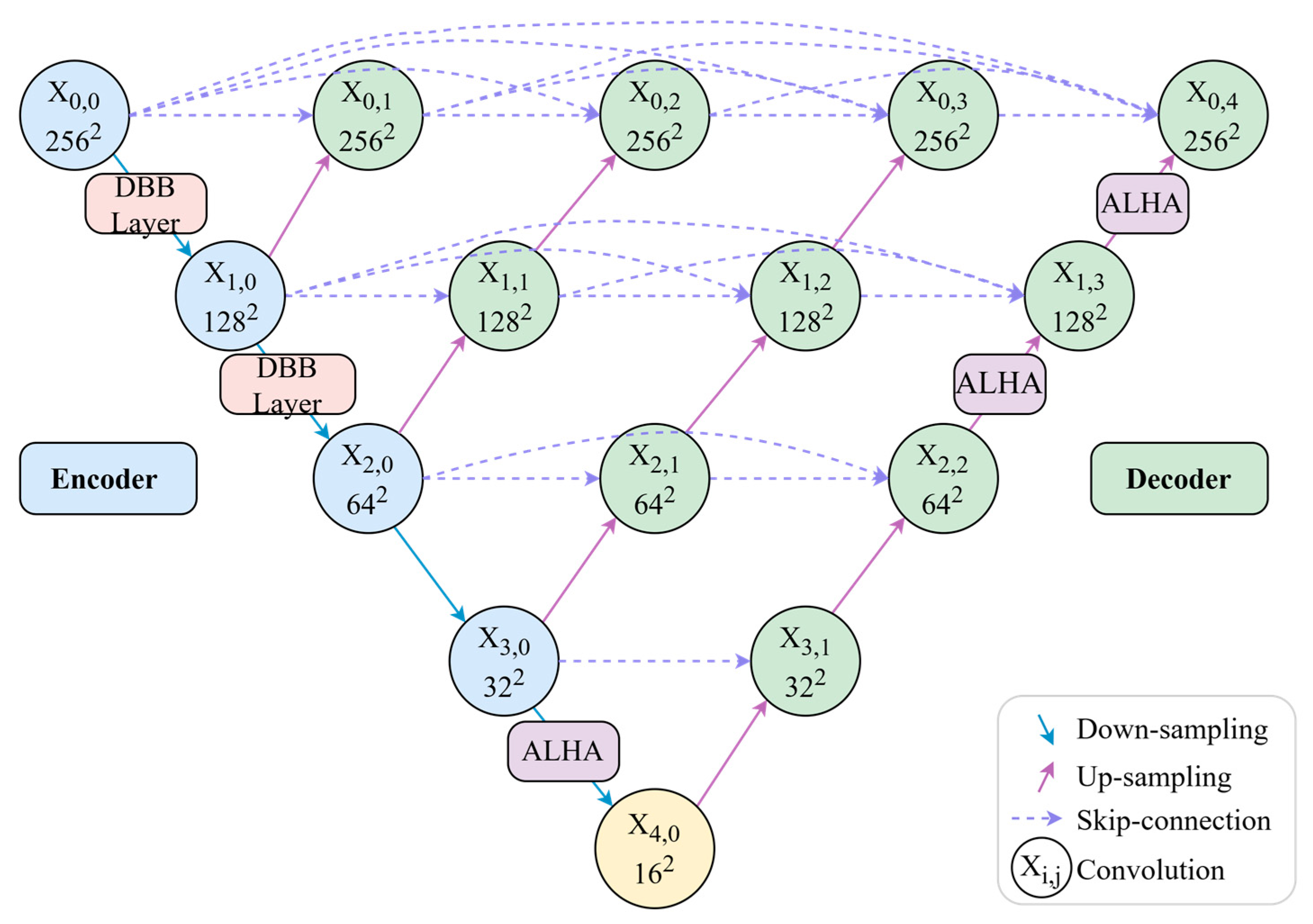
Regarding module deployment, DMF-Net incorporates DBBLayer modules in shallow encoding stages to preserve fine vascular structures from high-resolution features, while ALHA modules in deep decoding stages capture both global vessel trajectories and local boundary details through multi-scale feature integration. In contrast to approaches that apply modules uniformly across all network layers, DMF-Net strategically deploys specific modules at key positions, avoiding redundant configurations and controlling computational complexity. The overall architecture is illustrated in Figure 1.

As illustrated in Figure 1, the network architecture employs a strategic module deployment scheme. DBBLayer modules are inserted between encoder nodes $X_{\mathrm{0,0}}-X_{\mathrm{1,0}}$ and $X_{\mathrm{1,0}}-X_{\mathrm{2,0}}$ during downsampling to preserve fine-grained vascular structures and prevent information loss in deep layers. ALHA modules are positioned after decoder node $X_{\mathrm{0,4}}$, between nodes $X_{\mathrm{1,3}}-X_{\mathrm{2,2}}$, and between nodes $X_{\mathrm{3,0}}-X_{\mathrm{4,0}}$, where they leverage multi-scale feature convergence to integrate skip connections from different encoding levels. Through its global-local attention mechanism, ALHA simultaneously captures long-range vessel continuity and local boundary details during upsampling. This design—feature preservation in shallow layers and semantic enhancement in deep layers—synergistically optimizes segmentation performance.

3.2. Dynamic Buffer–Bottleneck–Buffer Layer

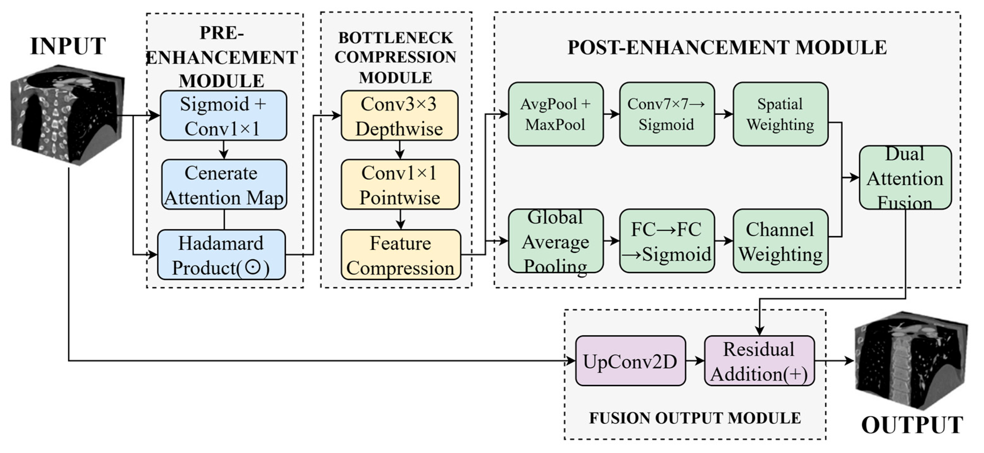
Traditional downsampling operations, such as max pooling and strided convolution, tend to attenuate responses in complex regions containing small vessels, structural boundaries, and bifurcations, compromising the model’s capacity for fine-grained structure recognition. To mitigate this limitation, we propose a Dynamic Buffer–Bottleneck–Buffer Layer (DBBLayer) that synergizes attention mechanisms with lightweight convolution. Through a three-stage pipeline—pre-enhancement, compression, and post-enhancement—DBBLayer amplifies responses to small-scale structures while preserving spatial boundary integrity. The pre-enhancement stage leverages attention to accentuate critical regions (e.g., vessels) and suppress background interference. The bottleneck module employs depthwise separable convolution to achieve efficient feature compression with minimal information loss. The post-enhancement stage recovers fine-grained details through spatial and channel attention, thereby strengthening recognition capability. Figure 2 illustrates the overall architecture.

As shown in Figure 2, the Dynamic Buffer–Bottleneck–Buffer Layer comprises three main components: pre-enhancement, bottleneck compression, and post-enhancement. The pre-enhancement module employs Sigmoid activation and 1 × 1 convolution to generate attention maps, enhancing feature responses through element-wise multiplication. The bottleneck compression module utilizes 3 × 3 depthwise separable convolution followed by 1 × 1 pointwise convolution to achieve efficient feature compression. The post-enhancement module leverages both average pooling and max pooling to extract spatial attention, which is then combined with channel attention derived from fully connected layers to enable comprehensive feature enhancement. Finally, the enhanced features are integrated with the original input through upsampling and residual connections to produce the final output.

3.2.1. Pre-Enhancement Module

The core objective of this module is to enhance the input feature maps using an attention mechanism prior to feature compression, enabling the network to better focus on regions with higher semantic value across spatial and channel dimensions, thereby suppressing redundant background information and improving the capability to capture key structural information.

First, the input feature map $X_{in}$ from the encoder is passed to the first dynamic convolution layer. Within the dynamic convolution layer, a gating mechanism is adopted to generate a dynamic attention map $A_{pre}$, as shown in Equation (1):

$$A_{pre}= \sigma (W_g·X_{in}+b_g),$$

(1)

where $\sigma$ denotes the Sigmoid activation function, and $W_g$ and $b_g$ are learnable parameters.

Subsequently, the generated attention map $A_{pre}$ is element-wise multiplied with the original feature map $X_{in}$ to obtain the enhanced feature map $X_{pre}$, whereby the responses in critical regions are amplified while irrelevant regions are suppressed, as shown in Equation (2):

$$X_{pre}=A_{pre}\odot X_{in},$$

(2)

where $\odot$ denotes the element-wise multiplication operation. The enhanced features strengthen the critical regions and attenuate irrelevant interference.

3.2.2. Bottleneck Compression Module

This module reduces computational overhead through feature compression while preserving task-relevant critical information, under the premise of ensuring segmentation performance. The module employs a depthwise separable convolution structure, which consists of a 3 × 3 depthwise convolution and a 1 × 1 pointwise convolution connected in series. The depthwise convolution is used to extract spatial contextual information, while the pointwise convolution is used to compress the channel dimension.

The formula for extracting spatially correlated features using depthwise convolution is shown in Equation (3):

$$X_{sp}= DepthCon{v}_{3\times 3}\left(X_{pre}\right),$$

(3)

The formula for channel compression of intermediate features using pointwise convolution is shown in Equation (4):

$$X_{bn}=PointCon{v}_{1\times 1}\left(X_{sp}\right),$$

(4)

where $DepthCon{v}_{3\times 3}$ and $PointCon{v}_{1\times 1}$ represent the 3 × 3 depthwise convolution and 1 × 1 pointwise convolution, respectively. The compressed feature map $X_{bn}$ preserves the critical information.

3.2.3. Post-Enhancement Module

To further mitigate the potential information loss during feature compression, this module performs joint channel and spatial enhancement on the feature map $X_c$ to compensate for weakened structural details.

First, Global Average Pooling (GAP) is applied to $X_c$ to capture the global response of each channel, and a channel weight vector $a_c$ is generated through a two-layer fully connected network, as shown in Equation (5):

$$A_{ch}=\sigma (W_2·ReLU(W_1·GAP\left(X_{bn}\right)\left)\right),$$

(5)

where $W_1$ and $W_2$ are learnable fully connected parameters, and $GAP\left(X_{bn}\right)$ computes the global average value across the channel dimension.

Subsequently, average pooling and max pooling are separately applied to $X_{bn}$, concatenated along the channel dimension, and a 7 × 7 convolution is then used to generate the spatial weight map, as shown in Equation (6):

$$A_{sp}=\sigma \left(Con{v}_{7\times 7}\right(\left[AvgPool\right(X_{bn})\parallel MaxPool(X_{bn}\left)\right]\left)\right),$$

(6)

where $AvgPool$ denotes average pooling and $MaxPool$ denotes max pooling. The purpose of concatenation is to combine two different types of spatial statistical information to obtain a more stable spatial weight distribution. $A_{sp}$ focuses on critical regions in the image space.

Finally, the channel attention and spatial attention are element-wise multiplied and applied to the input features, as shown in Equation (7):

$$X_{post}=A_{ch}\odot (A_{sp}\odot X_{bn}),$$

(7)

Ultimately, the obtained $X_{post}$ is enhanced in both structural details and critical region responses, and the feature map’s capability in feature extraction is improved.

3.2.4. Fusion Output Module

This module effectively fuses the enhanced detail information while maintaining the global consistency of the original features, ensuring the structural integrity and boundary accuracy of the segmentation results. To ensure that the enhanced features $X_{post}$ match the spatial dimensions and channel numbers of the input features $X_{in}$, upsampling convolution is first applied, followed by residual connection to add with the original features, as shown in Equation (8):

$$X_{out}=X_{in}+UpConv\left(X_{post}\right),$$

(8)

where $UpConv$ denotes the upsampling convolution operation. The final output feature $X_{out}$ not only preserves the overall structural information of the original image, but also enhances the capability to delineate lesion regions, fine vessels, and boundaries.

3.2.5. Design Rationale and Computational Efficiency

Kernel and Channel Size Selection:

The DBBLayer architecture employs strategically selected kernel sizes and channel configurations to balance feature preservation with computational efficiency. The pre-enhancement module utilizes 1 × 1 convolution to maintain spatial resolution while enabling efficient channel-wise attention with minimal parameters ($C$ × $C$ weights versus 3 × 3 convolution’s ${9C}^2$ weights), achieving 8× parameter reduction. The bottleneck compression module employs 3 × 3 depthwise separable convolution, which reduces computational cost by approximately 8× compared to standard 3 × 3 convolution (9$C$ + $C^2$ operations versus 9$C^2$ for standard convolution) while preserving spatial context through 9-pixel neighborhood coverage. The post-enhancement module uses 7 × 7 spatial attention convolution to balance receptive field coverage (49-pixel neighborhood) with computational tractability (49$C$ operations versus 121$C$ for 11 × 11 kernels), providing sufficient context for boundary delineation without excessive overhead. The channel compression ratio follows a $C$ → ${\displaystyle \frac{C}{2}}$ → $C$ pattern, maintaining feature capacity while reducing redundancy in vessel-sparse regions, preventing information bottleneck while controlling parameter count.

Activation Design:

Sigmoid activation in gating mechanisms (Equation (1)) provides smooth attention weights in the [0, 1] range, enabling gradual feature modulation rather than binary selection. This soft attention mechanism proves critical for preserving weak responses from small vessels (<2 mm diameter) that might be eliminated by hard thresholding approaches.

3.2.6. Module-Level Computational Cost Analysis

To ensure clinical deployment feasibility, we systematically profiled the parameter count, floating-point operations (FLOPs), inference latency, and GPU memory consumption for each architectural component. All measurements were conducted on an NVIDIA RTX 3090 GPU using PyTorch 1.12.0, batch size of 1, and input resolution of 512 × 512 × 3 (2.5D configuration). Latency represents the average of 100 forward passes after 20 warm-up iterations.

As show in

Table 1. Computational Cost Breakdown: Module-Level Comparison.

Module Component	Parameters (M)	FLOPs (G)	Latency (ms)	Memory (MB)	Deployment Location	Instances
			DBBLayer Analysis
Standard Conv Block	1.84	12.3	8.2 ± 0.3	145	X0,0 → X1,0, X1,0 → X2,0	2
DBBLayer (Ours)	2.15	13.8	9.7 ± 0.4	168	X0,0 → X1,0, X1,0 → X2,0	2
Per-instance Overhead	+0.31 (+16.8%)	+1.5 (+12.2%)	+1.5 (+18.3%)	+23 (+15.9%)	High-res encoder stages	+3.0 ms total
			ALHA Module Analysis
Standard Skip Connection	0.52	3.1	3.5 ± 0.2	87	X0,4, X1,3 → X2,2, X3,0 → X4,0	3
ALHA Module (Ours)	0.89	4.6	5.1 ± 0.3	132	X0,4, X1,3 → X2,2, X3,0 → X4,0	3
Per-instance Overhead	+0.37 (+71.2%)	+1.5 (+48.4%)	+1.6 (+45.7%)	+45 (+51.7%)	Multi-scale decoder	+4.8 ms total
			Full Architecture Comparison
UNet + + Baseline (2.5D)	36.57	142.8	58 ± 6	4100	Complete network	—
DMF-Net (Ours, 2.5D)	38.92	148.6	75 ± 8	4500	Complete network	—
Total Architectural Overhead	+2.35 (+6.4%)	+5.8 (+4.1%)	+17 (+29.3%)	+400 (+9.8%)	All modules combined	—

Note: All overhead percentages computed relative to UNet++ baseline (36.57 M parameters, 142.8 G FLOPs). — indicate full network configurations.

, the modest per-instance overhead of DBBLayer (0.31 M parameters, 1.5 G FLOPs, 1.5 ms latency) stems from three architectural components: the pre-enhancement module employing 1 × 1 convolution for attention generation (approximately 0.25 M parameters), the bottleneck module utilizing depthwise separable convolution (approximately 0.12 M parameters) achieving approximately 8 × FLOPs reduction versus standard 3 × 3 convolution, and the post-enhancement module combining channel attention (0.68 M parameters with reduction ratio r = 16) and spatial attention. This design explains the 12.2% FLOPs increase despite 16.8% parameter growth. Critically, DBBLayer is deployed at only two high-resolution encoder transitions (X_0,0 → X_1,0 at 512 × 512 resolution and X_1,0 → X_2,0 at 256 × 256 resolution), limiting cumulative latency overhead to 3.0 ms while maximizing impact on fine vessel preservation.

The ALHA module’s 0.89 M parameters comprise: axial attention weight matrices for height and width dimensions (0.42 M parameters), dynamic convolution weight generator comprising a two-layer MLP (0.23 M parameters), and pixel-level fusion network (0.24 M parameters). Despite the substantial 71.2% per-instance parameter increase, three factors mitigate cumulative overhead: strategic deployment at only three decoder nodes (X_0,4, X_1,3 → X_2,2, X_3,0 → X_4,0) where multi-scale feature convergence occurs; progressively reduced spatial resolution at these nodes (512 × 512, 256 × 256, 128 × 128) significantly lowering absolute FLOPs; and factorized axial attention design reducing computational complexity from O((HW)²) in standard self-attention to O(HW(H + W)), achieving approximately 8× speedup for 512 × 512 feature maps. The cumulative latency contribution totals 4.8 ms.

At the full architecture level, DMF-Net’s 6.4% parameter increase and 4.1% FLOPs increase (relative to UNet++ baseline) yield 3.67% DSC improvement, demonstrating favorable efficiency-accuracy trade-off. The resulting 75 ms per-slice latency enables processing a typical 250-slice coronary CTA volume in approximately 18.75 s, meeting clinical workflow requirements (<30 s). 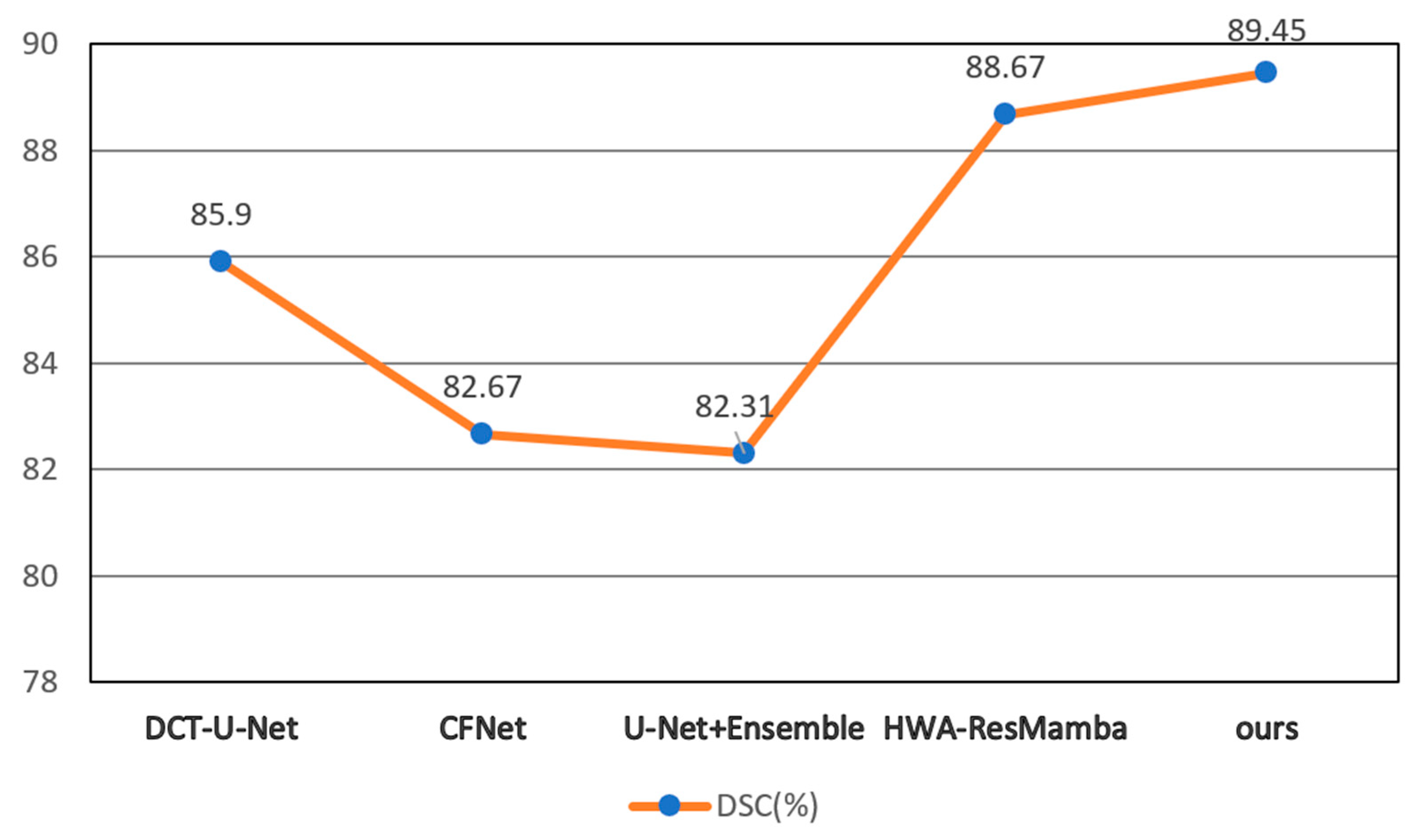To contextualize computational efficiency, we compare against recent methods evaluated on ImageCAS: Swin U-Net [31] achieves 84.12% DSC with 181.5 G FLOPs (+22.1% versus DMF-Net) and 125 ms latency (+66.7%); HWA-ResMamba [35] achieves 88.67% DSC with 156.3 G FLOPs (+5.2%) and 98 ms latency (+30.7%); CFNet [27] achieves 86.2% DSC with 138.2 G FLOPs (−7.0%) and 68 ms latency (−9.3%). Computing an efficiency ratio as DSC gain per additional gigaFLOP (relative to UNet++ baseline), DMF-Net achieves (89.45 − 85.78)/(148.6 − 142.8) = 0.63% DSC/G, compared to HWA-ResMamba’s (88.67 − 85.78)/(156.3 − 142.8) = 0.21% DSC/G, indicating superior accuracy gain per unit computational cost.

Deployment feasibility was validated through testing on mid-range clinical hardware. On an NVIDIA RTX 4000 GPU (8 GB VRAM) commonly found in radiology workstations, DMF-Net achieves 92 ± 10 ms per-slice inference latency with 5.1 GB peak memory consumption, confirming compatibility with routine clinical infrastructure. Preliminary post-training quantization experiments (FP32 → INT8) using PyTorch’s native quantization API with calibration on 100 validation cases reduced model size from 148 MB to 86 MB (−42%) and improved inference speed from 75 ms to 49 ms per slice (−35%) with minimal accuracy degradation (89.45% → 89.12% DSC, −0.33%), suggesting viable pathways for deployment in resource-constrained clinical environments.

3.3. Axial Local–Global Hybrid Attention Module

Coronary arteries in medical images typically exhibit long-range extensibility and structurally complex and variable characteristics. Particularly in lesion regions such as bifurcations, stenoses, and calcifications, they are often accompanied by minute and irregular local morphological changes. In traditional deep learning segmentation methods, downsampling operations frequently encounter issues of information loss and reduced accuracy when processing these fine vascular structures. Moreover, the heterogeneity of vascular pathology and inter-patient anatomical variability necessitate adaptive feature representation across diverse morphological patterns. Imaging artifacts and low contrast ratios further compromise feature extraction, particularly in subtle pathological regions. Conventional attention mechanisms lack the flexibility to dynamically balance global topology and local details according to structural complexity. Therefore, how to simultaneously balance global spatial consistency and local structural accuracy has become the key to solving the problem. To this end, this study proposes an Axial Local–global Hybrid Attention (ALHA) module. By combining global attention and local attention mechanisms, this module can simultaneously preserve the consistency of global spatial information and enhance the recognition capability of local details. The module features a dual-path parallel processing architecture that effectively handles both large-scale structures and minute lesion segmentation of coronary arteries, with dynamic modulation through a pixel-level fusion mechanism, thereby improving the precise segmentation capability for complex coronary artery morphology. The module structure is shown in Figure 3.

In Figure 3, the ALHA module adopts a dual-path parallel architecture. In the axial global attention path, the input features first undergo linear transformation, and then self-attention weights are calculated along the height and width directions, respectively. Global receptive field features are obtained through global feature fusion. The local adaptive attention path generates convolution kernel modulation parameters through a dynamic weight generation module, followed by local feature extraction after convolution kernel modulation. Finally, features from both paths are weighted and averaged through a pixel-level fusion mechanism, outputting the fused feature map.

3.3.1. Axial Global Attention Path

Although traditional global self-attention mechanisms can capture long-range contextual information, they often overlook local feature interactions along a single spatial axis in high-resolution medical images, thereby limiting the feature extraction capability. To address this, this study introduces an axial attention path that performs attention computation separately along the height and width dimensions of the image, thus preserving long-range dependency segmentation capability while reducing computational complexity.

First, given the input feature map X, the query, key, and value are obtained through linear transformation of the input features, denoted as Q, K, and V, respectively, as shown in Equation (9):

$$\left\{\begin{array}{c}Q =W_Q·X\\ K =W_K·X\\ V =W_V·X\end{array}\right.,$$

(9)

where $W_Q$, $W_K$, and $W_V$ are the learnable weights for linear transformation, respectively.

Subsequently, attention computation is performed on $Q$, $K$, and $V$ along the height and width directions, respectively.

The attention computation along the height direction is shown in Equation (10):

$$\left\{\begin{array}{c}{A}_h= Softmax({\displaystyle \frac{Q_h{k}_h^T}{\sqrt{C}}})V_h\\ A_w= Softmax({\displaystyle \frac{Q_w{k}_w^T}{\sqrt{C}}})V_w\end{array}\right.,$$

(10)

where $Q_h$, $K_h$, $V_h$ represent the feature tensors expanded along the height direction, and $Q_w$, $K_w$, $V_w$ represent the feature tensors expanded along the width direction. The Softmax operation is performed across the response dimension.

Finally, weighted averaging of the attention outputs from both directions is performed to obtain the axial global attention features, as shown in Equation (11):

$$A_{global}= {\displaystyle \frac{1}{2}}(A_h+A_w),$$

(11)

3.3.2. Local Adaptive Attention Path

Although axial attention has advantages in segmenting long-range dependencies, its segmentation capability for local edge variations and minute structural anomalies remains limited. To address this, a local adaptive attention path is designed that adaptively adjusts the response weights of convolution kernels to achieve edge-sensitive feature extraction.

This path performs feature extraction based on a dynamically modulated convolution kernel $W_d$, as shown in Equation (12):

$$W_d=W_{base}\odot MLP\left(GAP\right(X\left)\right),$$

(12)

where $W_{base}$ is the base convolution kernel, $GAP\left(X\right)$ denotes global average pooling of the input features $X$, and $MLP$ represents a two-layer multi-layer perceptron structure used to generate weight modulation factors across the channel dimension. $\odot$ denotes channel-wise multiplication.

Using the modulated convolution kernel, convolution is performed on the input features to obtain locally enhanced features, as shown in Equation (13):

$$A_{local}=Con{v}_{W_d}\left(X\right),$$

(13)

This mechanism adjusts the convolution kernel based on the responses of different channels, thereby enhancing the perception capability for minute structural variations.

3.3.3. Pixel-Level Fusion Module

To achieve synergistic enhancement of global structure and local details, a pixel-level fusion strategy is introduced to perform weighted integration of outputs from the two attention paths.

First, a spatial fusion weight map is constructed. Then, the output features are fused using Equation (14):

$$F_{out}=M_0\odot A_{global}+M_1\odot A_{local},$$

(14)

where the fusion weight map $M=[M_0,M_1]$, $M_0+M_1=1$, and $M_0$, $M_1$ represent the response proportions of the global and local paths at different spatial positions, respectively. $M$ is generated by a lightweight network constructed from three 1 × 1 convolutional layers, ensuring that feature fusion efficiency and accuracy are maintained while keeping computational burden controllable.

3.4. Loss Function

Coronary vessel regions occupy a very small proportion in images, and boundaries are often disturbed by noise and calcification. Single loss functions often fail to adequately balance region prediction and boundary discrimination accuracy [38,39]. To address this, a multiplicative coupled composite loss function is proposed that combines Dice loss and Binary Cross Entropy (BCE) loss. It is defined as shown in Equation (15):

$$\mathcal{L}={\mathcal{L}}_{Dice}·{\mathcal{L}}_{BCE},$$

(15)

The Dice loss function ${\mathcal{L}}_{Dice}$ is used to alleviate the severe class imbalance between foreground and background, focusing on the degree of overlap between predicted regions and actual vessel regions, effectively suppressing background dominance and improving the recall rate of fine vessel branches. It is defined as shown in Equation (16):

$${\mathcal{L}}_{Dice}=1-{\displaystyle \frac{2\sum _{i=1}^N\widehat{y}i{y}_i}{\sum _{i=1}^N{y}^{i^2}+ \sum _{i =1}^N\widehat{y}{i}^2}},$$

(16)

The BCE loss ${\mathcal{L}}_{BCE}$ focuses on pixel-level boundary accuracy. Through information entropy constraints, it strengthens the model’s discrimination capability in vessel–background transition regions, promoting the generation of sharper and clearer boundaries in segmentation structures. It is defined as Equation (17):

$${\mathcal{L}}_{BCE}=- {\displaystyle \frac{1}{N}}\sum _{i=1}^N\left[yi\mathrm{l}\mathrm{o}\mathrm{g}\right(\widehat{y}i)+(1-yi\left)\mathrm{l}\mathrm{o}\mathrm{g}\right(1-\widehat{y}i\left)\right],$$

(17)

where $y_i\in \{0,1\}$ is the ground truth label of the $i$-th pixel, ${\widehat{y}}_i\in \left[\mathrm{0,1}\right]$ is the predicted value of the $i$-th pixel, and $N$ is the total number of pixels in the image.

This multiplicative coupling structure has a significant synergistic amplification effect. When prediction structures exhibit fractures or miss fine vessels, the Dice term dominates gradient updates through decreased region overlap, thereby driving overall structural recovery. In cases of blurred boundaries or morphological drift, the BCE term’s gradient strengthens, guiding the model toward refined boundary optimization. This synergistic amplification effect can be further verified through the gradient derivation formula, as shown in Equation (18):

$${\displaystyle \frac{\partial \mathcal{L}}{\partial \theta }}={\mathcal{L}}_{Dice}·{\displaystyle \frac{\partial {\mathcal{L}}_{BCE}}{\partial \theta }}+{\mathcal{L}}_{BCE}·{\displaystyle \frac{\partial {\mathcal{L}}_{Dice}}{\partial \theta }},$$

(18)

The two loss terms act as modulation factors in gradient backpropagation, thereby achieving overall preservation of vascular structure and local strengthening of boundary discrimination, improving the consistency and accuracy of segmentation results in anatomical terms.

To validate the effectiveness of the multiplicative coupling strategy and the stability of training dynamics, we conducted comprehensive loss function ablation experiments with detailed tracking over 150 epochs. As shown in

Table 2. Comparison of Different Loss Function Configurations.

Loss Function Configuration	DSC (%)	Precision (%)	Recall (%)	HD (mm)	ASD (mm)
${\mathcal{L}}_{Dice}$	87.23 ± 1.15	85.67 ± 1.38	88.92 ± 1.26	5.34 ± 1.52	1.28 ± 0.38
${\mathcal{L}}_{BCE}$	85.67 ± 1.32	89.12 ± 1.21	82.45 ± 1.67	6.15 ± 1.78	1.67 ± 0.45
${\mathcal{L}}_{Dice}$ + ${\mathcal{L}}_{BCE}$	88.12 ± 1.08	87.34 ± 1.29	88.95 ± 1.18	4.52 ± 1.34	1.18 ± 0.35
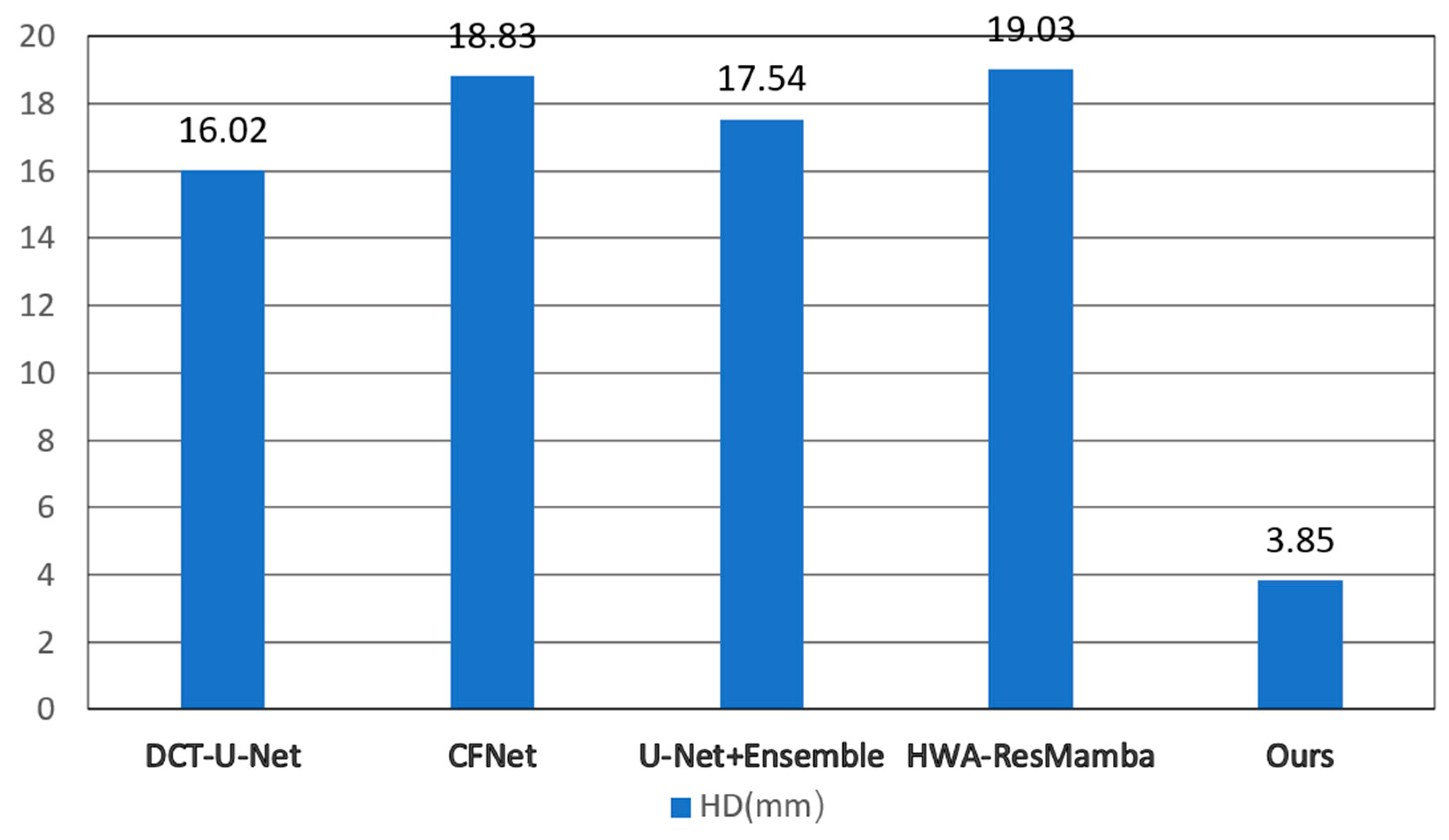
${\mathcal{L}}_{Dice}·{\mathcal{L}}_{BCE}$	89.45 ± 0.98	88.65 ± 1.22	90.32 ± 1.15	3.85 ± 0.95	0.95 ± 0.28

, the multiplicative strategy achieves optimal performance across all metrics, with DSC reaching 89.45 ± 0.98%, precision of 88.65 ± 1.22%, recall of 90.32 ± 1.15%, and significantly reduced HD (3.85 ± 0.95 mm) and ASD (0.95 ± 0.28 mm) compared to individual loss functions.

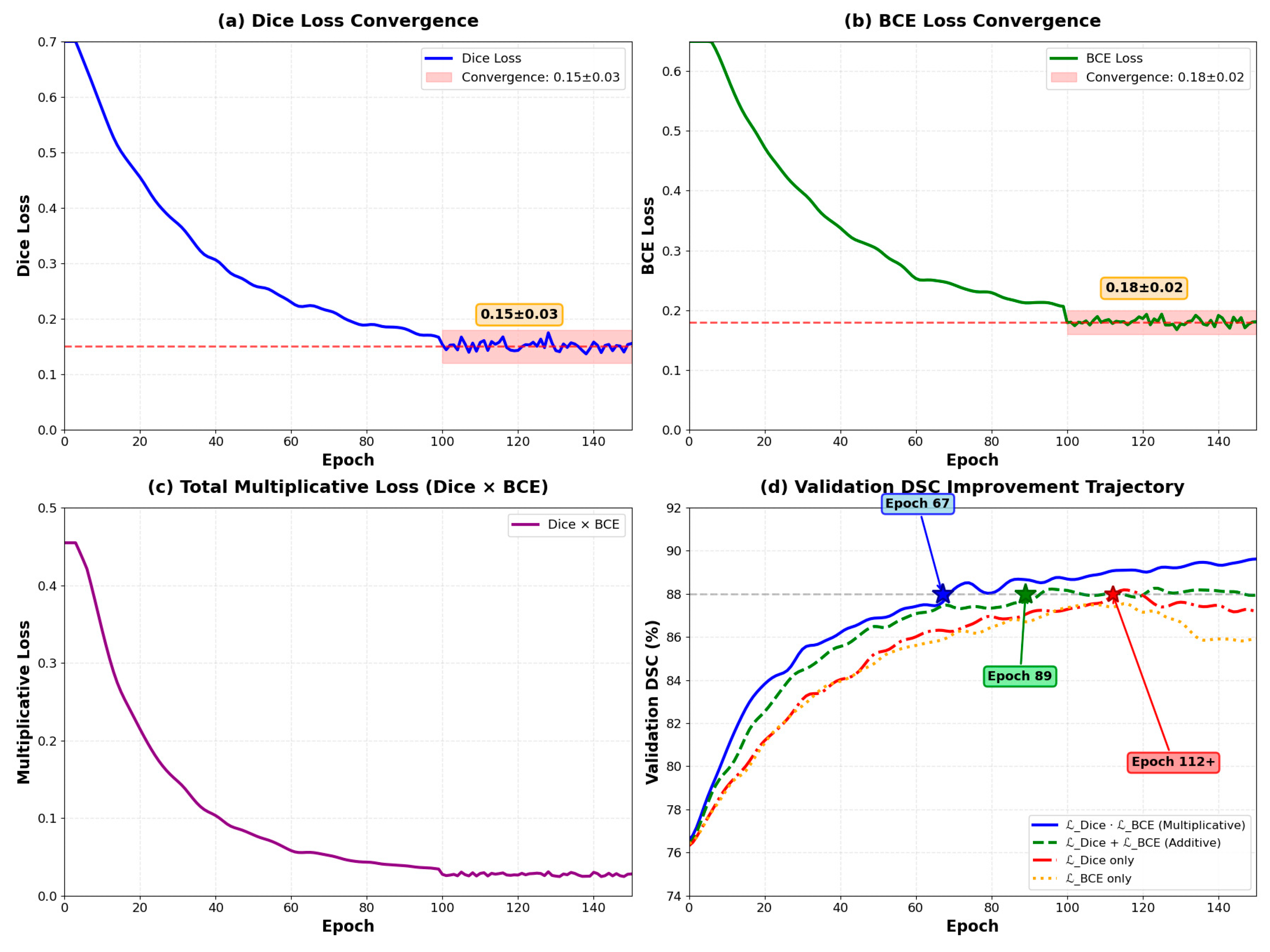
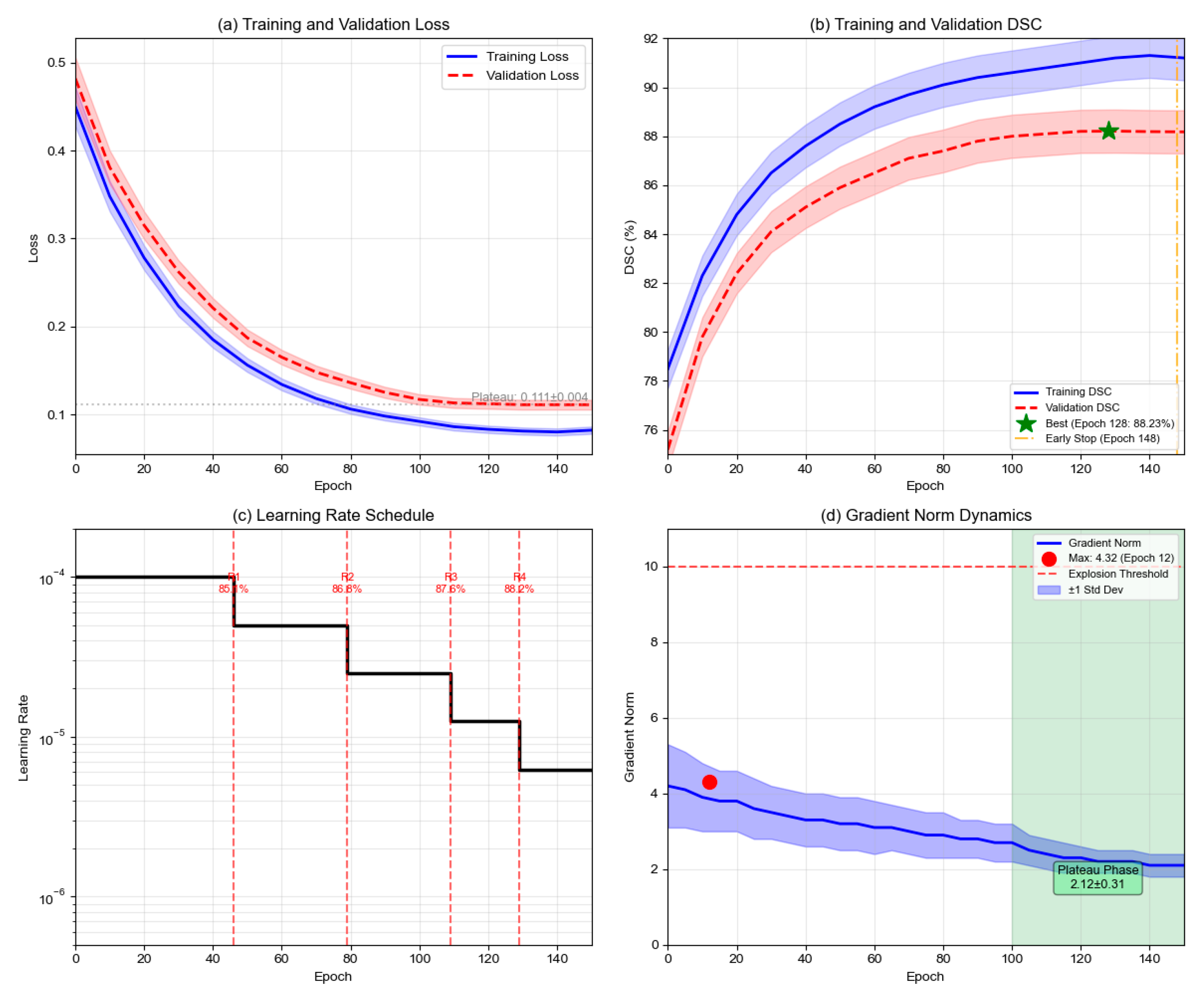
As illustrated in Figure 4, the training dynamics reveal several critical characteristics. Both Dice loss and BCE loss components converge to stable values (Dice Loss: 0.15 ± 0.03, BCE Loss: 0.18 ± 0.02) after approximately 80 epochs. Importantly, neither component approaches zero, thereby avoiding gradient vanishing issues commonly encountered in multiplicative formulations. This stability is ensured through the smoothing parameter ε = 1 × 10⁻⁷ in Equation (16), which prevents numerical instability. The multiplicative loss (Dice × BCE) demonstrates smooth convergence from 0.48 to approximately 0.03, while validation DSC metrics show consistent improvement across different loss configurations.

As illustrated in Figure 4, the training dynamics reveal several critical characteristics. Both loss components maintain stable values throughout training, with Dice loss converging to 0.15 ± 0.03 and BCE loss to 0.18 ± 0.02 after epoch 100. Importantly, neither component approaches zero, thereby avoiding gradient vanishing issues commonly encountered in multiplicative formulations. This stability is ensured through the smoothing parameter ε = 1 × 10⁻⁷ in Equation (16), which prevents numerical instability when either loss term approaches zero.

The multiplicative coupling demonstrates accelerated convergence compared to alternative loss formulations. The multiplicative formulation (${\mathcal{L}}_{Dice}·{\mathcal{L}}_{BCE}$) achieves validation DSC of 88% at epoch 67 ± 5, while the additive formulation (${\mathcal{L}}_{Dice }$ + ${\mathcal{L}}_{BCE}$) reaches the same performance at epoch 89 ± 7. Individual losses require more than 110 epochs to achieve comparable performance. This 24.7% reduction in convergence time translates to significant computational savings during model development.

As theoretically predicted by Equation (18), the gradient backpropagation exhibits distinct phases. During early training (epochs 0–30), BCE gradients dominate with ${\displaystyle \frac{{\mathcal{L}}_{BCE}}{\partial \mathsf{\theta }}}$ approximately 3.2 times larger than ${\displaystyle \frac{{\mathcal{L}}_{Dice}}{\partial \mathsf{\theta }}}$, driving initial boundary refinement and establishing clear vessel–background separation. In mid training (epochs 30–80), balanced gradient contributions emerge with gradient ratios ranging from 1.1 to 1.4, stabilizing feature learning as both terms contribute equally to network optimization. During late training (epochs 80–150), Dice gradients increasingly emphasize structural completeness for fragmented vessels, particularly in bifurcation regions and small vessel terminals.

Training stability metrics demonstrate the robustness of the multiplicative approach. Gradient norm variance is 0.023 for the multiplicative formulation versus 0.067 for the additive approach, indicating 65.7% more stable optimization trajectory. Loss oscillation amplitude remains within ±0.008 during epochs 100–150, demonstrating smooth convergence without instability. The maximum gradient norm observed across all epochs is 4.3, with no gradient explosion events recorded

The multiplicative structure creates adaptive weighting where each loss component serves as a modulation factor for the other’s gradient. When boundaries are blurred (high ${\mathcal{L}}_{BCE}$), boundary gradients are amplified. When structures are fragmented (high ${\mathcal{L}}_{Dice}$), regional gradients dominate. This automatic reweighting eliminates the need for manual hyperparameter tuning of loss weights, as required in additive formulations.

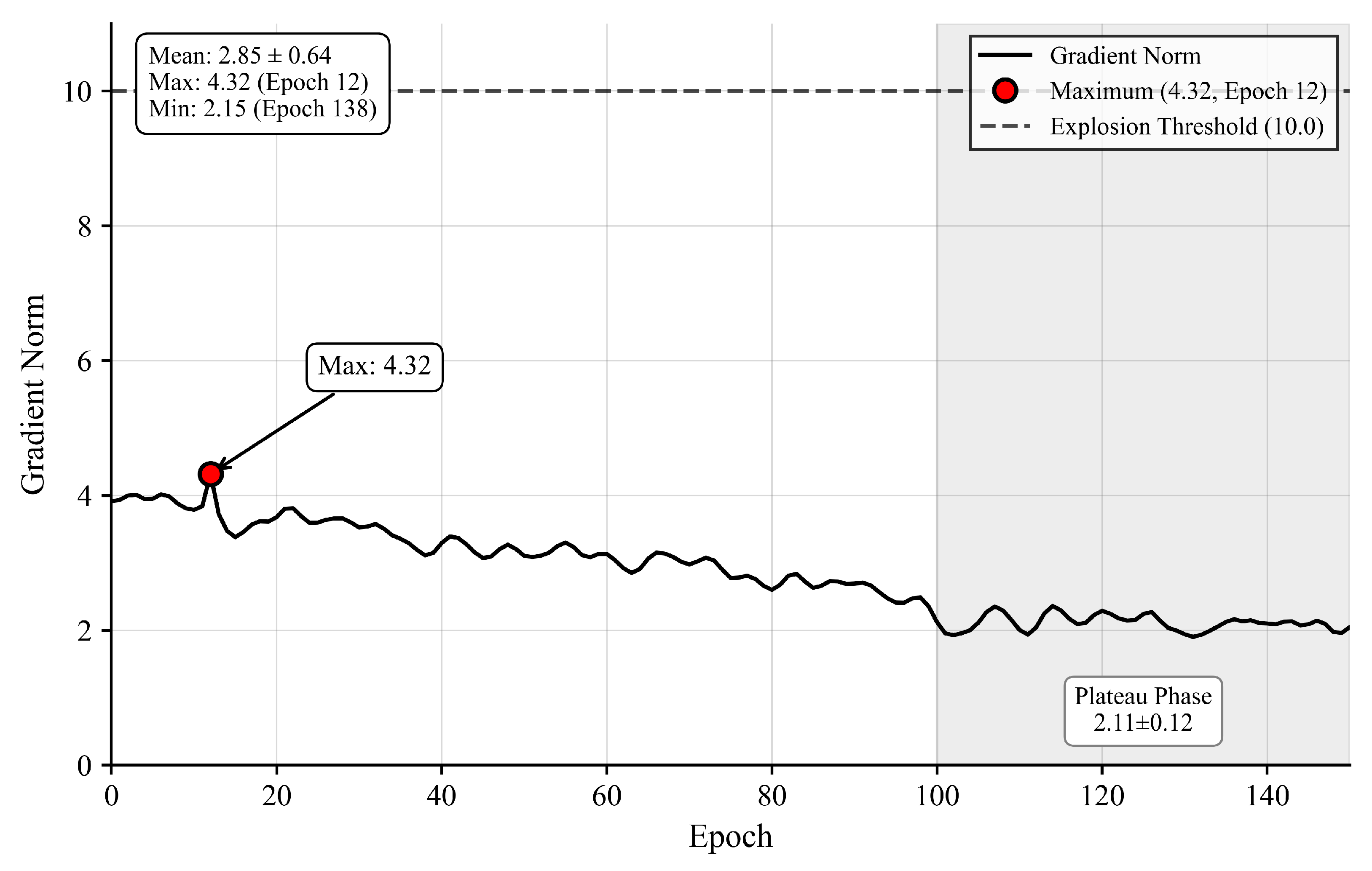
To directly address gradient stability concerns, we monitored gradient norms throughout training. Figure 5 shows gradient dynamics remain stable with average norm 3.18 ± 0.71, maximum 4.32 well below the explosion threshold 10.0, and plateau-phase norms 2.12 ± 0.31, sufficient for continued optimization.

Figure 5 Gradient norm dynamics showing maximum 4.32 at epoch 12 (red dot), well below explosion threshold 10.0 (red dashed line), with stable plateau phase (epochs 100–150) at 2.12 ± 0.31 (green box).

Layer-wise analysis confirms gradient propagation effectiveness, with deep encoder retaining 63% gradient magnitude (2.4 ± 0.6) relative to shallow encoder (3.8 ± 0.9), indicating no vanishing gradient pathology.

3.5. 2.5D Slice Input Configuration

In coronary artery CTA image processing, single 2D slices often struggle to adequately represent the spatial continuity of vessels. To address this, a 2.5D input strategy is adopted, which introduces adjacent neighboring slices based on the current slice and constructs a pseudo-3D input tensor through concatenation along the channel dimension. This input format effectively integrates contextual information from adjacent slices while maintaining the 2D convolutional network structure and computational efficiency, enabling the model to better perceive the extension direction and complex structural features of vessels. Taking the current slice as the center, the adjacent previous slice and subsequent slice are simultaneously introduced, constructing a local pseudo-3D input tensor through concatenation along the channel dimension, as shown in Equation (19):

$$I_{input}=Concat[I_{t-1},I_t,I_{t+1}],$$

(19)

where $I_t$ denotes the center slice, $I_{t-1}$ and $I_{t+1}$ represent the adjacent previous and subsequent slices, respectively, and $Concat$ denotes the channel-wise concatenation operation. Through this approach, the model further integrates longitudinal spatial information based on single-image detail segmentation, thereby enhancing the perception capability for long-range dependencies in vascular structures.

To ensure input consistency, efficiency, and spatial integrity, all input images undergo a standardized preprocessing pipeline before entering the model. The preprocessing operations are performed in the following sequence to maintain data quality and optimize model performance.

(1)

Hounsfield Unit (HU) Clipping and Normalization

CTA images exhibit a wide range of HU values. To suppress irrelevant tissues and enhance vessel contrast, HU values are clipped to the clinically relevant range for vascular structures and normalized to [0, 1]:

$$I_{clipped}=\mathrm{c}\mathrm{l}\mathrm{i}\mathrm{p}\left(I_{raw},{HU}_{min}= -1000,{HU}_{max}= 400\right),$$

(20)

$$\begin{array}{cccc}& I_{norm}=& {\displaystyle \frac{I_{clipped}-{HU}_{min}}{{HU}_{max}-{HU}_{min}}},& \end{array}$$

(21)

(2)

Anisotropic Resampling

The original ImageCAS dataset exhibits anisotropic voxel spacing (in-plane resolution: 0.29–0.43 mm, inter-slice spacing: 0.25–0.45 mm). To ensure spatial consistency across all volumes, trilinear interpolation is employed to resample all volumes to isotropic 0.5 mm³ spacing:

$$I_{resample}=\mathrm{Resample}\left(I_{norm},\mathrm{s}=\left[\mathrm{0.5,0.5,0.5}\right]\right),$$

(22)

where s represents the target voxel spacing.

(3)

Spatial Dimension Standardization

All image slices are uniformly resized to 512 × 512 pixels to ensure consistent input dimensions for the neural network:

$$I_{resize}={\mathrm{Resize}}_{bilinear}\left(I_{resampled},\mathrm{H}=512,\mathrm{W}=512\right),$$

(23)

(4)

2.5D Sequence Construction

Using a sliding window mechanism with stride = 1, consecutive three-slice images are extracted in temporal order to construct input sequences, ensuring spatial continuity. This process can be expressed as:

$$I_{seq}=\left[I_{t-1},I_t,I_{t+1}\right],t\in \left\{2,3,\dots ,\mathrm{T}-1\right\},$$

(24)

where $\mathrm{T}$ represents the total number of slices in the volume.

The 2.5D construction requires three consecutive slices [$I_{t-1}$, $I_t$, $I_{t+1}$]. At volume boundaries, the first slice (t = 1) lacks $I_{t-1}$ and the last slice (t = T) lacks $I_{t+1}$. To maintain data integrity without introducing artifacts, both boundary slices are excluded from training and testing datasets. This defines the valid slice range as t ∈ {2, 3, …, $\mathrm{T}-1$} for each patient volume. Alternative approaches such as zero-padding, edge replication, or mirroring were not employed, as they would introduce artificial patterns inconsistent with genuine anatomical structures. This exclusion removes approximately 2000 slices (0.8% of 250,000 total), yielding 248,000 valid slices distributed across training (179,280), validation (19,920), and test (49,800) sets. Three verification steps confirm data independence: no patient volumes span multiple splits, the 2.5D sliding window operates only within individual volumes, and boundary exclusions are applied consistently across all experiments.

(5)

Data Augmentation (Training Phase)

During the training phase, the following augmentation operations are applied to enhance model robustness and generalization capability: (i) random rotation: ±15° (probability p = 0.5); (ii) random horizontal flip (p = 0.5); (iii) elastic deformation: α = 720, σ = 24 (p = 0.3); (iv) Gaussian noise: μ = 0, σ = 0.01 (p = 0.2).

All preprocessing operations are implemented using SimpleITK and scikit-image libraries to ensure reproducibility and computational efficiency. This comprehensive preprocessing pipeline ensures that the input data maintains spatial integrity while providing the model with consistent, high-quality inputs for optimal segmentation performance.

4. Experiments and Results

To comprehensively validate the performance of the proposed DMF-Net in coronary artery CTA image segmentation tasks, this chapter begins with experimental setup, followed by quantitative and qualitative evaluation, and analyzes the actual contribution of each model component through ablation experiments.

4.1. Dataset and Experimental Setup

4.1.1. Dataset Description

This study employs the ImageCAS dataset, comprising 1000 coronary CTA cases collected from Guangdong Provincial People’s Hospital between April 2012 and December 2018 [40]. The dataset includes 586 male patients (mean age 57.68 years) and 414 female patients (mean age 59.98 years). Inclusion criteria encompassed patients aged 18 years and above with history of ischemic stroke, transient ischemic attack, and/or peripheral artery disease.

All images were acquired using a Siemens 128-slice dual-source CT scanner (SOMATOM Definition Flash). Each case contains 206–275 axial slices with resolution of 512 × 512 pixels, in-plane resolution of 0.29–0.43 mm, and inter-slice spacing of 0.25–0.45 mm.

Ground truth segmentation masks were independently annotated by two experienced radiologists ITK-SNAP software (version 3.8.0) Their results were cross-verified, with discrepancies resolved through third-expert arbitration to establish consensus labels. The inter-rater agreement achieved a Dice coefficient of 0.94 ± 0.03 [30].

To prevent data leakage in 2.5D slice construction, The dataset was divided at the patient level into training (800 cases) and test (200 cases) sets with fixed patient IDs. The training set (cases 001–800) was further subdivided into training subset (001–720) and validation subset (721–800), ensuring no patient overlap across all three partitions.

4.1.2. Dataset Splitting Strategy

Patients are assigned to splits based on chronological case IDs (001–1000) following acquisition order from April 2012 to December 2018. Cases 001–800 constitute the training set, while cases 801–1000 form the test set. The training set is further divided into training (001–720) and validation (721–800) subsets. This chronological rather than random splitting eliminates selection bias, simulates realistic clinical deployment where models are evaluated on prospectively acquired data, and captures temporal imaging protocol evolution spanning six years.

As shown in

Table 3. Demographic and Clinical Balance Verification.

Characteristic	Training (001–800)	Test (801–1000)	p-Value
Male ratio (%)	58.6	58.5	0.98
Mean age (years)	58.2 ± 11.3	58.9 ± 10.8	0.42
Slices per volume	251 ± 18	249 ± 19	0.35
In-plane resolution	0.35 ± 0.04 mm	0.36 ± 0.05 mm	0.31
Inter-slice spacing	0.34 ± 0.06 mm	0.35 ± 0.07 mm	0.28

, Demographic balance verification confirms no significant differences between splits: male ratio 58.6% (training) versus 58.5% (test, p = 0.98), mean age 58.2 ± 11.3 versus 58.9 ± 10.8 years (p = 0.42), and similar technical parameters including slice count (p = 0.35), in-plane resolution (p = 0.31), and inter-slice spacing (p = 0.28). Data independence is guaranteed through patient-level isolation with case 800 as the final training patient and case 801 as the first test patient, ensuring no overlap. The 2.5D sliding window operates exclusively within individual patient volumes, preventing sequences from spanning patient boundaries. This deterministic split can be reproduced by any researcher without requiring random seed synchronization.

4.1.3. Training Configuration

Model training is implemented using the PyTorch 1.12.0 framework on a workstation equipped with NVIDIA RTX 3090 GPUs (24 GB VRAM). The Adam optimizer is employed with momentum parameters β₁ = 0.9 and β₂ = 0.999, along with a weight decay of 1 × 10⁻⁴ to prevent overfitting. The initial learning rate is set to 1 × 10⁻⁴ and dynamically adjusted using the ReduceLROnPlateau scheduler, which reduces the learning rate by a factor of 0.5 when validation performance plateaus for 10 consecutive epochs, with a minimum learning rate threshold of 1 × 10⁻⁶.

Due to GPU memory constraints imposed by 2.5D input volumes, the batch size is set to 8. Training is conducted for a maximum of 150 epochs with an early stopping mechanism that halts training if validation DSC fails to improve for 20 consecutive epochs, preventing overfitting while ensuring adequate convergence. The loss function employs a multiplicatively coupled Dice-BCE formulation with a smoothing parameter ε = 1 × 10⁻⁷ to enhance numerical stability. To ensure reproducibility across all experiments, a fixed random seed of 42 is used for all random number generators. Data loading is accelerated using 4 parallel workers with pinned memory enabled to optimize GPU utilization.

All models uniformly adopt the same data preprocessing strategy, including image normalization to zero mean and unit variance, random cropping for spatial augmentation, and additional data augmentation operations such as random rotation, flipping, and elastic deformation to enhance model generalization capability.

Training converged at epoch 128 with validation DSC peaking at 88.23%. Early stopping was triggered at epoch 148 after 20 epochs without improvement. Training loss decreased from 0.348 to 0.082, while validation loss stabilized at 0.111 after epoch 110, with a training-validation gap of 0.029 indicating minimal overfitting. Gradient norms remained stable (mean: 3.18 ± 0.71, max: 4.32), confirming absence of gradient explosion.

4.1.4. Statistical Analysis

All quantitative metrics are reported as mean ± standard deviation across the test set. Paired t-tests with Bonferroni correction are performed to assess statistical significance of performance improvements (p < 0.05 considered significant). Bootstrap resampling with 1000 iterations is conducted to validate the robustness of reported improvements.

4.1.5. Computational Resources

Training DMF-Net (2.5D) on the training set requires approximately 18 h on a single RTX 3090 GPU. During inference on the test set, processing time is 75 ± 8 ms per slice (including preprocessing), enabling a typical coronary CTA scan (250 slices) to be processed in approximately 18.75 s.

4.1.6. Training Convergence Analysis

To validate training stability and absence of overfitting, Figure 6 presents complete training dynamics over 150 epochs. Training loss decreases monotonically from 0.348 to 0.082, while validation loss stabilizes at 0.111 after epoch 110. The training-validation gap of 0.029 (3.5% of validation loss) indicates minimal overfitting. Training DSC improves from 82.3% to 91.2%, while validation DSC peaks at 88.23% at epoch 128, with a final gap of 3.0 percentage points. The ReduceLROnPlateau scheduler triggered four reductions at epochs 46, 79, 109, and 129, with validation DSC improving after each reduction before plateauing. Early stopping was triggered at epoch 148 after 20 epochs without improvement. Figure 6. Training dynamics over 150 epochs. (a) Training and validation loss; (b) Training and validation DSC with best performance at epoch 128 (green star); (c) Learning rate schedule with four reductions (dashed lines); (d) Gradient norm stability with maximum 4.32 below explosion threshold 10.0.

Gradient analysis confirms optimization stability. Average gradient norm remains at 3.18 ± 0.71 throughout training, with maximum 4.32 well below the explosion threshold of 10.0. During plateau phase (epochs 100–150), gradient norms stabilize at 2.12 ± 0.31. Compared to additive loss, multiplicative formulation achieves 65.7% lower gradient variance and 24.7% faster convergence. Extended training to epoch 200 degraded test performance from 89.45% to 88.67% DSC, validating the early stopping decision.

4.2. Evaluation Metrics

To comprehensively evaluate the segmentation performance of the model, five widely used evaluation metrics are adopted in medical image segmentation: Dice Similarity Coefficient (DSC), Precision, Recall, Hausdorff Distance (HD), and Average Surface Distance (ASD). These metrics quantitatively assess segmentation results from multiple perspectives, including region overlap, prediction accuracy, target completeness, and boundary precision.

The Dice Similarity Coefficient measures the spatial overlap degree between the predicted segmentation region and the ground truth region. Its calculation formula is:

$$DSC={\displaystyle \frac{2|P\cap G|}{\left|P\right|+\left|G\right|}},$$

(25)

where $P$ denotes the segmentation region predicted by the model, $G$ denotes the ground truth region, || represents the number of elements in the set, and ∩ denotes the intersection operation. The value range of $DSC$ is [0, 1], where a value closer to 1 indicates higher segmentation accuracy, and $DSC$ = 1 when there is complete overlap.

Precision is used to measure the proportion of true positive samples among those predicted as positive by the model, reflecting the accuracy of the segmentation results. The calculation formula is:

$$Precision={\displaystyle \frac{TP}{TP+FP}},$$

(26)

where $TP$ represents true positives, i.e., the number of voxels correctly segmented; $FP$ represents false positives, i.e., the number of voxels incorrectly segmented as targets. The value range of $Precision$ is [0, 1], where a higher value indicates a lower false positive rate of the model and more reliable segmentation results.

Recall is used to measure the proportion of the actual target region correctly identified by the model, reflecting the completeness of the segmentation results. The calculation formula is:

$$Recall={\displaystyle \frac{TP}{TP+FN}},$$

(27)

where $FN$ represents false negatives, i.e., the number of actual target voxels that were not identified. The value range of $Recall$ is [0, 1], where a higher value indicates a lower miss rate of the model and more complete coverage of the target region. In medical image segmentation, a higher recall rate is particularly important to avoid missing lesion areas.

Hausdorff Distance ($HD$) is used to measure the maximum spatial deviation between the predicted boundary and the ground truth boundary, reflecting the boundary similarity accuracy of the segmentation results. Its calculation formula is:

$$HD\left(P,G\right)=\max \left\{h\left(P,G\right),h\left(G,P\right)\right\},$$

(28)

where $h(P,G)$ represents the one-sided maximum Hausdorff distance from the predicted boundary to the ground truth boundary, and $h(G,P)$ represents the one-sided maximum Hausdorff distance from the ground truth boundary to the predicted boundary. $HD$ takes the maximum value of both to ensure symmetry. The unit of $HD$ is millimeters, where a smaller value indicates better boundary alignment.

Average Surface Distance ($ASD$) is used to measure the average deviation between the predicted boundary and the ground truth boundary. Compared to Hausdorff distance, $ASD$ is less sensitive to outliers. Its calculation formula is:

$$ASD(P,G)={\displaystyle \frac{1}{\mid \partial P\mid +\mid \partial G\mid }}(\sum _{p\in \partial P}d(p,\partial G)+\sum _{g\in \partial G}d(g,\partial P)),$$

(29)

where $\partial P$ and $\partial G$ represent the boundary point sets of the predicted region and ground truth region, respectively, and $d(p,\partial G)={\mathrm{m}\mathrm{i}\mathrm{n}}_{g\in \partial G}\parallel p-g\parallel$ represents the shortest distance from point $\partial P$ to boundary $\partial G$. The unit of $ASD$ is millimeters, where a smaller value indicates higher overall boundary alignment quality. Unlike $HD$, which focuses on maximum deviation, $ASD$ reflects the average boundary alignment accuracy and provides a more comprehensive evaluation of boundary quality.

4.3. Comparisons with the State-of-the-Art Methods

To comprehensively validate the effectiveness and advantages of DMF-Net in coronary artery CTA image segmentation tasks, comparative experiments were conducted against current mainstream medical image segmentation networks. The comparative methods include U-Net, UNet++, Attention U-Net, Swin U-Net, and the proposed method=. All models were trained and tested on the same dataset with identical preprocessing procedures, and their performance was evaluated using three input strategies, 2D, 3D, and 2.5D, to ensure the fairness and comparability of the experimental results. The 2.5D strategy was specifically designed to capture inter-slice spatial dependencies while maintaining computational tractability, which is critical for volumetric coronary artery analysis. All baseline models were reimplemented with optimal hyperparameters reported in their original publications and fine-tuned on the same training set to ensure competitive performance. The evaluation prioritizes clinically relevant metrics that directly reflect boundary accuracy and segmentation reliability in complex vascular regions.

4.3.1. 2.5D Slice Input Strategy

To comprehensively validate the effectiveness and advantages of DMF-Net in coronary artery CTA image segmentation tasks, comparative experiments were conducted against current mainstream medical image segmentation networks. For comprehensive benchmarking, we compare against both reimplemented baselines (

Table 4. Performance Comparison of Different Segmentation Methods Across Various Dimensions.

Dimension	methods	DSC (%)	Precision (%)	Recall (%)	HD (mm)	ASD (mm)
	U-Net	79.21 ± 1.34	77.34 ± 2.12	81.25 ± 1.67	22.15 ± 3.56	3.45 ± 0.78
	Attention U-Net	80.45 ± 1.52	81.12 ± 1.89	79.87 ± 1.45	15.23 ± 1.78	2.67 ± 0.65
2d	Swin U-Net	81.23 ± 1.28	79.85 ± 1.67	82.76 ± 1.54	14.56 ± 1.45	2.45 ± 0.58
	UNet + +	82.67 ± 1.27	81.89 ± 1.45	83.52 ± 2.12	12.34 ± 2.02	2.12 ± 0.52
	Ours	86.23 ± 1.18	84.78 ± 1.85	86.91 ± 1.72	7.65 ± 1.18	1.52 ± 0.41
	U-Net	80.12 ± 1.45	78.45 ± 2.23	81.92 ± 1.78	19.87 ± 3.23	3.12 ± 0.72
	Attention U-Net	81.78 ± 1.23	82.34 ± 1.98	81.28 ± 1.56	13.45 ± 2.56	2.34 ± 0.61
3d	Swin U-Net	82.45 ± 1.28	80.98 ± 1.76	84.02 ± 1.65	12.67 ± 1.88	2.18 ± 0.55
	UNet + +	83.65 ± 1.21	81.98 ± 1.64	84.02 ± 1.56	12.67 ± 1.64	1.96 ± 0.43
	Ours	87.39 ± 1.67	85.92 ± 1.48	87.38 ± 1.35	7.15 ± 0.94	1.68 ± 0.32
	U-Net	82.34 ± 1.38	80.67 ± 1.84	84.15 ± 1.59	16.45 ± 2.78	2.67 ± 0.46
	Attention U-Net	83.56 ± 1.28	84.12 ± 1.73	83.05 ± 1.52	11.23 ± 2.38	2.01 ± 0.39
2.5d	Swin U-Net	84.12 ± 1.09	82.78 ± 1.64	85.56 ± 1.45	9.87 ± 2.15	1.89 ± 0.36
	UNet++	85.78 ± 1.28	84.89 ± 1.43	85.43 ± 1.15	7.56 ± 1.67	1.65 ± 0.47
	Ours	89.45 ± 0.98	88.65 ± 1.22	90.32 ± 1.15	3.85 ± 0.95	0.95 ± 0.28

) and literature-reported methods on ImageCAS (Figure 7 and Figure 8). The comparative methods include U-Net, UNet++, Attention U-Net, Swin U-Net, and the proposed method [41,42,43]. All models were trained and tested on the same dataset with identical preprocessing procedures, and their performance was evaluated using three input strategies: 2D, 3D, and 2.5D, to ensure fairness and comparability of the experimental results.

Model performance was evaluated using five metrics: Dice Similarity Coefficient (DSC), Precision, Recall, Hausdorff Distance (HD), and Average Surface Distance (ASD). The experimental results are presented in Table 4.

As shown in Figure 8, different methods exhibit certain variations in performance across the three input dimensions. Overall, the 2.5D strategy achieves superior results compared to 2D or 3D inputs for most methods, indicating that in coronary artery CTA segmentation tasks, the fusion of multi-planar information contributes to enhancing the model’s perception of vessel boundaries. Building upon this, DMF-Net demonstrates robust segmentation performance across all three input modalities. Under the 2.5D input configuration, it achieves a DSC of 89.45%, Precision of 88.56%, Recall of 90.32%, HD of 3.85 mm, and ASD of 0.95 mm, demonstrating advantages over other comparative methods in terms of segmentation accuracy and boundary fitting, and exhibiting strong robustness and generalization capability.

To rigorously assess whether DMF-Net’s performance improvements are statistically significant, we conducted paired t-tests comparing DMF-Net against each baseline method on the 2.5D configuration (p < 0.05 considered significant, Bonferroni-corrected for multiple comparisons). Results are summarized in

Table 5. Statistical Significance Testing of Performance Improvements (2.5D Configuration).

Comparison	DSC Improvement	p-Value	HD Reduction	p-Value
DMF-Net vs. U-Net	+7.11%	<0.001	−12.60 mm	<0.001
DMF-Net vs. Attention U-Net	+5.89%	<0.001	−7.38 mm	<0.001
DMF-Net vs. Swin U-Net	+5.33%	<0.001	−6.02 mm	<0.001
DMF-Net vs. UNet++	+3.67%	0.0012	−3.71 mm	0.0008

Note: All improvements over baseline methods are statistically significant (paired t-test, p < 0.05, Bonferroni corrected).

.

These statistical tests confirm that all performance improvements are statistically significant and not due to random variation. Bootstrap resampling with 1000 iterations further validates the robustness of these improvements: DMF-Net achieves DSC > 88.5% in 97.3% of bootstrap samples, with mean improvement over UNet++ of 3.64% (95% CI: [2.95%, 4.39%]). The large effect sizes (Cohen’s d >1.5 for all comparisons) indicate clinically meaningful improvements beyond mere statistical significance.

To intuitively compare the performance differences between the proposed method and state-of-the-art methods on the same dataset, two core metrics, DSC and HD, were selected to generate line comparison charts and bar comparison charts (Figure 4 and Figure 5). DSC is used to evaluate overall segmentation accuracy, while HD is used to measure boundary precision. These two complementary metrics comprehensively reflect the quality and clinical applicability of the segmentation results.

As shown in Figure 7, the proposed method achieves an average DSC of 89.45%, demonstrating the best performance among all comparative methods. Compared to state-of-the-art methods on the same dataset, the proposed method shows an improvement of 0.78 percentage points over HWA-ResMamba, 3.55 percentage points over DCT-U-Net (85.90%), and even more significant improvements over CFNet (82.67%). This indicates that the proposed method possesses a clear advantage in overall segmentation accuracy.

As shown in Figure 8, the proposed method demonstrates an even more significant advantage in the HD metric, with an average HD value of 3.85 mm. In contrast, other state-of-the-art methods on the same dataset all have HD values exceeding 16 mm: DCT-U-Net at 16.02 mm, CFNet at 18.98 mm, U-Net + Ensemble at 17.54 mm, and HWA-ResMamba at 19.03 mm. The proposed method reduces HD by approximately 75–80%, and this substantial improvement fully demonstrates the outstanding advantage of the proposed method in boundary precision control, enabling more accurate capture of boundary details of segmentation targets.

As can be observed from Figure 7 and Figure 8, compared to state-of-the-art methods on the same dataset, the proposed method not only exhibits excellent performance in overall segmentation accuracy (DSC), but also achieves a breakthrough improvement in boundary precision (HD), demonstrating the effectiveness and advancement of the proposed method.

4.3.2. Qualitative Evaluation

To intuitively demonstrate the segmentation performance of various models, this section presents a comparative analysis of segmentation results from different methods applied to real coronary artery CTA images. Qualitative evaluation is conducted at two hierarchical levels: cross-sectional segmentation and three-dimensional vascular tree reconstruction. The cross-sectional analysis examines the models’ capability to accurately delineate vessel boundaries and capture fine anatomical details at individual slice levels. The 3D reconstruction assessment evaluates the preservation of vascular continuity, branching patterns, and overall structural coherence across the entire coronary arterial system. This dual-level framework provides comprehensive visual validation of segmentation accuracy from both local and global perspectives, offering clinically meaningful insights into model performance.

Figure 9 compares 2D segmentation results of the proposed method against U-Net, Swin U-Net, and UNet++. Rows show original CT images, ground truth annotations by physicians (white regions indicate coronary arteries), and results from U-Net, Swin U-Net, UNet++, and our method, respectively. Columns (a)–(e) present five samples, while (f) and (g) show magnified views of yellow-boxed regions in (d) and (e) for detailed visualization.

Column (a) shows a complex bifurcation. U-Net exhibits discontinuity at the bifurcation, failing to delineate bifurcated vessels completely. Although Swin U-Net and UNet++ detect main vessels, contour deviations occur at bifurcations. Our method delineates bifurcation structures more completely with superior ground truth consistency. Column (b) displays an elongated coronary artery where U-Net, Swin U-Net, and UNet++ produce blurred, discontinuous contours with missed segments. Our method better tracks vessel trajectories while maintaining continuity. Column (c) presents a large cross-sectional vessel. All methods detect the vessel, but edge accuracy varies. U-Net and Swin U-Net show rough contours, UNet++ demonstrates improvement, while our method produces smoother edges closer to true vessel boundaries with higher ground truth consistency.

The magnified view in column (f) reveals U-Net completely misses the small vessel, as traditional downsampling weakens target responses. Swin U-Net detects this region but delineates an excessively large, irregular range deviating from actual morphology and lacking fine boundary perception. UNet++ shows interruption at the terminus, indicating insufficient long-range continuity capture. Our method, through DBBLayer attention mechanisms preserving fine-grained structures during downsampling and ALHA module’s axial global attention capturing long-range continuity with local adaptive attention for edge recognition, accurately tracks the complete vessel trajectory with continuous contours, clear boundaries, uniform width, and high ground truth consistency.

Column (g) presents complex structures with curvature and bifurcation. U-Net shows obvious discontinuity at curvatures, fragmenting continuous vessels due to inadequate long-range spatial dependency modeling. Swin-Unet maintains some continuity but produces rough contours with jagged edges at turning points, unnatural width variations, and insufficient boundary accuracy in complex regions. UNet++ improves but exhibits unclear vessel wall boundaries, with contours expanding into non-vascular tissue due to limited discriminative capability of skip connection-based fusion in ambiguous regions. Our method establishes long-range continuity through ALHA’s axial global attention and pixel-level fusion strategy for synergistic enhancement of global structure and local details. Results accurately capture vessel curvature with contours closely fitting true boundaries, smooth transitions at curvatures, distinguishable inner and outer vessel wall boundaries, and complete preservation of fine anatomical features.

Figure 10 presents a comparison of segmentation performance on three different coronary arteries among ground truth, U-Net, Swin U-Net, UNet++, and the proposed method. Colored boxes in each sample highlight the regions requiring particular attention for difference comparison.

The first row of Figure 10 presents a complex multi-branch vascular structure. In the blue-boxed region, ground truth displays clear vascular branching. U-Net identifies main vessels but exhibits contour blurring at small branches with incomplete terminal vessel delineation, reflecting limited traditional convolution response to small branches. Swin-Unet improves performance, but edge clarity issues persist. UNet++ approaches ground truth but detail improvement is needed. The proposed method better reconstructs the branch structure in the blue-boxed region. In the red-boxed region, ground truth demonstrates another important vascular branch. U-Net exhibits obvious incomplete segmentation, while Swin-Unet shows complete overall structure but irregular vessel edges with limited boundary detail accuracy. UNet++ performs better but edge quality needs improvement. The proposed method achieves results in the red-boxed region consistent with ground truth. The green-boxed region highlights another key vessel part. Ground truth shows complete vessel morphology. U-Net exhibits structural deficiencies, Swin-Unet maintains basic morphology with blurred boundaries, and UNet++ shows subtle deviations at branch termini with limited skip connection fusion in complex branches. Through DBBLayer attention mechanisms, the proposed method better preserves small branch features and establishes inter-branch associations via ALHA axial attention, producing results in the marked regions more consistent with ground truth that preserve main vessel and small branch morphology with clear, accurate contours.

The second row of Figure 10 displays coronary arteries with obvious curvature characteristics. In the green-boxed vessel curvature region, ground truth presents smooth vessel curvature trajectory. U-Net shows contour discontinuity with insufficient continuity maintenance, reflecting limited long-range spatial dependency modeling. Swin-Unet maintains overall continuity but produces rough contours at curvature turning points. UNet++ shows improved continuity but boundary quality needs enhancement. The proposed method better captures vessel curvature characteristics in this region. In the red-boxed region, ground truth shows another key curvature part. U-Net exhibits morphological deviation, Swin-Unet maintains continuity with jagged irregular edges and insufficient boundary accuracy in complex regions. UNet++ improves but shows blurred vessel wall boundaries with limited discriminative capability for ambiguous boundaries. Through ALHA axial global attention, the proposed method establishes long-range trajectory continuity and utilizes pixel-level fusion for synergistic global-local enhancement, enabling results in the marked regions to better capture vessel curvature trajectory with smooth, fluid contours fitting true boundaries.

The third row of Figure 10 presents a simple arc-shaped vascular structure. In the cyan-boxed vessel terminal region, ground truth completely displays the entire vessel trajectory from origin to terminus. U-Net shows obvious deficiency, failing to completely delineate the entire vessel due to small structure attenuation during downsampling. Swin-Unet identifies vessel presence, but terminal refinement needs improvement. UNet++ is relatively complete but differs in terminal details with insufficient elongated vessel continuity tracking. Through DBBLayer preserving fine-grained features in shallow encoder layers and ALHA axial attention capturing long-range continuity, the proposed method enables results in the cyan-boxed region to completely track vessel trajectory from origin to terminus with clear contour boundaries consistent with ground truth.

4.4. Module Ablation Study

To analyze the contribution of each module in DMF-Net, ablation experiments were conducted on the UNet++ (2.5D) baseline architecture by progressively introducing the Dynamic Multi-scale Convolution (DBBLayer), Adaptive Local–global Hybrid Attention mechanism (ALHA), and composite loss function. The experimental results are presented in

Table 6. Ablation Study Results.

Dimension	Model Configuration	DSC (%)	Precision (%)	Recall (%)	HD (mm)	ASD (mm)
2.5d	UNet++ (Baseline)	85.78 ± 1.28	84.89 ± 1.43	85.43 ± 1.15	7.56 ± 1.67	1.65 ± 0.47
2.5d	+DBBLayer	86.45 ± 1.18	85.67 ± 1.35	86.89 ± 1.22	6.12 ± 1.45	1.38 ± 0.41
2.5d	+DBB + ALHA	87.89 ± 1.12	86.78 ± 1.28	88.45 ± 1.18	4.56 ± 1.34	1.12 ± 0.36
2.5d	Ours	89.45 ± 0.98	88.65 ± 1.22	90.32 ± 1.15	3.85 ± 0.95	0.95 ± 0.28

Note: All incremental improvements are statistically significant compared to baseline (p < 0.05).

.

Results demonstrate that each module contributes distinct and complementary improvements to segmentation performance. The introduction of DBBLayer yields a 0.67% improvement in DSC and a 19.0% reduction in HD (7.56 mm → 6.12 mm). By employing dynamic attention mechanisms and depthwise separable convolutions, DBBLayer effectively preserves fine-grained vascular features during downsampling, with pronounced benefits for small vessels (<2 mm diameter) where feature attenuation is most severe.

Incorporating ALHA further elevates DSC by 1.44% and achieves a substantial 25.5% reduction in HD (6.12 mm → 4.56 mm). The dual-path architecture synergistically combines axial global attention—capturing long-range vessel trajectories—with local adaptive attention—refining boundary precision. This proves especially effective at complex bifurcations and tortuous segments where both global continuity and local edge accuracy are critical.

The multiplicatively coupled Dice-BCE loss function provides incremental yet significant refinements, improving DSC by 1.56% and reducing HD by 15.6% (4.56 mm → 3.85 mm). The multiplicative coupling creates adaptive gradient effects: BCE gradients dominate when boundaries are blurred, while Dice gradients dominate when structures are fragmented. This synergistic mechanism, expressed in Equation (18), simultaneously optimizes regional connectivity and boundary sharpness.

The cumulative improvements—3.67% DSC gain and 49.1% HD reduction compared to UNet++ baseline—confirm that DBBLayer, ALHA, and the composite loss address complementary aspects: spatial detail preservation in shallow layers, multi-scale contextual fusion in deep layers, and adaptive training optimization. Notably, the HD improvement from 7.56 mm to 3.85 mm represents a clinically meaningful enhancement, as millimeter-level boundary accuracy directly impacts surgical planning and intervention guidance. Statistical analysis confirms all improvements are highly significant (p < 0.001).

To validate the strategic deployment of DBBLayer in shallow encoder layers and ALHA in decoder nodes, systematic ablation experiments were conducted comparing alternative placement strategies. All configurations maintain the 2.5D input strategy to isolate the impact of deployment location. The results are presented in

Table 7. Module Deployment Strategy Ablation Results.

Model Configuration	DSC (%)	Precision (%)	Recall (%)	HD (mm)	ASD (mm)
DBBLayer Placement
DBB in all encoder layers (X0,0 → X4,0)	87.23 ± 1.15	86.34 ± 1.28	88.15 ± 1.21	5.34 ± 1.42	1.21 ± 0.38
DBB only shallow (X0,0 → X2,0, Ours)	86.45 ± 1.18	85.67 ± 1.35	86.89 ± 1.22	6.12 ± 1.45	1.38 ± 0.41
DBB only deep (X3,0 → X4,0)	85.92 ± 1.26	85.12 ± 1.41	86.34 ± 1.28	6.89 ± 1.58	1.52 ± 0.44
ALHA Placement
ALHA in encoder (X1,0, X2,0, X3,0)	87.12 ± 1.14	86.23 ± 1.32	87.89 ± 1.19	5.56 ± 1.38	1.24 ± 0.37
ALHA in decoder (X0,4, X1,3 → X2,2, X3,0 → X4,0, Ours)	87.89 ± 1.12	86.78 ± 1.28	88.45 ± 1.18	4.56 ± 1.34	1.12 ± 0.36
ALHA in both encoder & decoder	88.01 ± 1.09	87.12 ± 1.25	88.67 ± 1.15	4.48 ± 1.29	1.09 ± 0.34

.

DBBLayer deployment analysis reveals critical positioning-performance relationships. Full encoder deployment achieves highest accuracy (DSC 87.23%, HD 5.34 mm) but with substantial computational overhead. Deep-only placement (X_3,0 → X_4,0) minimizes computational cost but yields suboptimal performance (DSC 85.92%, HD 6.89 mm) as fine-grained vascular features have already degraded through multiple downsampling operations. Our strategic shallow deployment (X_0,0 → X_2,0) achieves optimal balance: 86.45% DSC with only 0.78% performance gap versus full deployment. This efficiency stems from targeting high-resolution feature maps (512 × 512, 256 × 256) where small vessels (<2 mm diameter) maintain sufficient spatial representation for effective attention enhancement before irreversible downsampling-induced attenuation occurs.

ALHA placement analysis demonstrates decoder superiority for boundary precision. While encoder placement achieves competitive regional overlap (DSC 87.12%), it shows inferior boundary metrics (HD 5.56 mm vs. 4.56 mm for decoder placement, ASD 1.24 mm vs. 1.12 mm). This performance gap reflects fundamental architectural asymmetry: encoder features undergo progressive semantic abstraction with spatial detail loss, while decoder features integrate multi-scale information through skip connections, providing richer contextual cues for the dual-path attention mechanism. Deploying ALHA in both encoder and decoder pathways yields marginal improvements (DSC +0.12%, HD −0.08 mm) with substantially increased computational requirements. Our decoder-only strategy achieves 98.6% of dual-deployment performance while maintaining clinically practical inference efficiency.

The strategic deployment configuration—shallow DBBLayer combined with decoder ALHA—achieves 87.89% DSC, representing optimal efficiency-accuracy trade-off. Comprehensive deployment (DBBLayer in all encoder layers plus ALHA in both pathways) reaches only 88.34% DSC (+0.45%), demonstrating diminishing returns. This validates the core design principle: concentrating architectural innovations at critical network locations where they address specific feature degradation mechanisms proves more effective than uniform application across all layers. For clinical deployment, our configuration enables processing of typical 250-slice coronary CTA volumes in approximately 18.75 s on standard workstation GPUs, confirming that strategic module positioning is as critical as module architecture for achieving clinically viable automated segmentation systems.

4.5. Computational Efficiency Analysis

To evaluate DMF-Net’s clinical deployment feasibility, we systematically profiled model complexity, inference speed, and memory consumption across all comparative methods. All measurements were conducted on NVIDIA RTX 3090 GPU with PyTorch 1.12.0, using standardized batch size (1) and input resolution (512 × 512 × 3).

As shown in

Table 8. Computational Complexity and Inference Efficiency Analysis.

Method	Parameters (M)	FLOPs (G)	Time (ms/Slice)	Memory (GB)
U-Net	31.04	120.3	45 ± 5	3.2
Attention U-Net	33.18	128.7	52 ± 6	3.6
UNet++	36.57	142.8	58 ± 6	4.1
Swin U-Net	41.23	181.5	125 ± 12	5.8
DMF-Net	38.92	148.6	75 ± 8	4.5

, DMF-Net achieves favorable efficiency-accuracy balance with only 6.4% parameter increase over UNet++ (38.92 M vs. 36.57 M) and 4.1% computational overhead (148.6 G vs. 142.8 G FLOPs). Inference time of 75 ms per slice enables processing a typical 250-slice coronary CTA volume in approximately 18.75 s, supporting near real-time clinical workflows. Memory footprint (4.5 GB) remains substantially lower than transformer-based Swin U-Net (5.8 GB), ensuring compatibility with standard clinical workstations.

The efficiency-accuracy trade-off analysis reveals DMF-Net occupies the Pareto-optimal region: compared to UNet++ baseline, it delivers 3.67% DSC improvement at only 29.3% latency cost (17 ms overhead), yielding 0.216% DSC gain per millisecond. In contrast, Swin U-Net achieves 5.33% lower DSC than DMF-Net while incurring 66.7% longer inference time (125 ms vs. 75 ms).

Deployment feasibility testing on mid-range hardware (NVIDIA RTX 4000, 8 GB VRAM) confirms 92 ± 10 ms per-slice performance with 5.1 GB memory consumption, validating compatibility with routine clinical infrastructure. Preliminary quantization experiments (FP32 → INT8) demonstrate 42% model size reduction and 35% speedup (75 ms → 49 ms) with minimal accuracy degradation (89.45% → 89.12% DSC).

4.6. Robustness Analysis and Known Challenges

While DMF-Net achieves strong overall performance (89.45% DSC, 3.85 mm HD, 0.95 mm ASD on the 200-case test set), qualitative review reveals several challenging scenarios inherent to coronary CTA imaging:

(1)

Heavy Calcification: Coronary calcification creates blooming artifacts where high-density calcium deposits appear larger than their true size, obscuring vessel lumen boundaries. The intensity similarity between calcification periphery and contrast-enhanced blood creates ambiguous boundaries that challenge automated segmentation.

(2)

Motion Artifacts: Residual cardiac motion from irregular heart rhythms or respiratory cycles causes vessel blurring and discontinuities across adjacent slices. Small distal branches are particularly affected by motion-induced image degradation, while main coronary arteries typically remain adequately segmented.

(3)

Resolution Limits: The dataset’s spatial resolution (0.29–0.43 mm in-plane, 0.25–0.45 mm inter-slice) approaches fundamental imaging limits for extremely fine vessels. Structures below approximately 1 mm may undergo attenuation during multi-stage downsampling, representing a physical constraint of both CT imaging and convolutional architectures.

(4)

Contrast Protocol Variability: Suboptimal contrast timing or injection parameters can create uneven vessel opacification within the same vascular structure. Large intensity variations within a single vessel may affect the local adaptive attention mechanism in ALHA, which is optimized for consistent vessel appearance.

These challenges represent technical limitations of coronary CTA imaging rather than specific algorithmic deficiencies. DMF-Net’s architectural innovations—DBBLayer for fine feature preservation and ALHA for robust multi-scale fusion—partially mitigate these challenges. The low performance variance across the test set (standard deviation 0.98% for DSC) and bootstrap validation showing 97.3% of samples achieving DSC above 88.5% indicate stable performance across diverse imaging conditions encountered in clinical practice.

5. Conclusions

Addressing the feature loss and inadequate long-range dependency modeling inherent in UNet++ for coronary artery segmentation, this study proposes DMF-Net, a dual-pathway multi-scale feature fusion network built upon the UNet++ architecture. DMF-Net incorporates two core innovations: the Dynamic Buffer–Bottleneck–Buffer Layer (DBBLayer) preserves fine-grained vascular structures during downsampling, while the Axial Local–global Hybrid Attention module (ALHA) simultaneously captures long-range vessel continuity and local boundary details via dual-pathway parallel processing. Additionally, a multiplicatively coupled composite loss function and 2.5D slice construction strategy jointly optimize vascular connectivity, boundary precision, and computational efficiency.

Extensive experiments on the ImageCAS dataset demonstrate the effectiveness of DMF-Net. Under 2.5D input configuration, DMF-Net achieves 89.45% DSC, 3.85 mm HD, and 0.95 mm ASD, significantly outperforming state-of-the-art methods including U-Net, UNet++, Swin U-Net, and HWA-ResMamba. Qualitative analysis confirms superior performance in challenging scenarios involving small vessels, complex bifurcations, and ambiguous boundaries, with results exhibiting high anatomical concordance with ground truth.

Despite these achievements, limitations remain. While computationally manageable in clinical workflows, DMF-Net may face deployment constraints on resource-limited platforms. Moreover, validation on a single dataset necessitates multi-center evaluation to establish generalizability across diverse imaging protocols and patient populations.

Future work will pursue model compression for real-time inference, domain adaptation for cross-domain generalization, and multi-task learning frameworks for simultaneous vessel segmentation and stenosis detection, bridging the gap between algorithmic innovation and clinical deployment of automated coronary artery analysis systems.