Parametric Inner Bounds for the Extreme Eigenvalues of Real Symmetric Matrices

Abstract

Here, inner bounds for the extreme eigenvalues of a real symmetric matrix are derived by using a two-dimensional subspace of ${\mathbb{R}}^n$. The addition of a single parameter to the basis vectors and optimization thereof results in superior bounds, as compared to using fixed basis vectors. This is a rather simple procedure that is easily automated.

1. Introduction

The determination of the spectrum $\sigma \left(\mathbf{A}\right)$ matrix is a fundamental problem in almost all spheres of science. In fact, if the eigenpairs are known, then this is a complete description of the associated linear operator. In most cases, the solution of the characteristic equation $det(\lambda \mathbf{I}-\mathbf{A})=0$ is unmanageable for large matrix dimensions n. In this case, numerical methods suffice, for example, the $QR$ algorithm [1]. In some cases, it is only the location of the spectrum that is required, whilst in other instances, knowledge of the extreme eigenvalues is sufficient. Weinstein bounds [2] and Kato bounds [3] depend on an approximate eigenpair, which may be evaluated numerically. For real symmetric matrices, Lehmann’s method [4] provides both upper and lower bounds for the eigenvalues. The Temple quotient [5] provides a lower bound for the smallest eigenvalue of such a matrix and is a special case of Lehmann’s method. Brauer [6] provides a method to calculate the outer bounds for $\sigma \left(\mathbf{A}\right)$ for such matrices. The Rayleigh quotient [7] is often used when some approximate eigenpair is known to improve the eigenvalue. The Gerschgorin theorem and ovals of Cassini [8] depend only on knowledge of the entries of a matrix, yet they yield powerful results, especially for large sparse matrices. Trace bounds use only the diagonal elements of a matrix; however, they can yield some very impressive bounds for the eigenvalues. These have been studied extensively by Wolcowicz and Styan [9]. Sharma et al. [10] extended and improved the work of Wolcowiz and Styan, whilst Singh et al. [11,12] generalized the work of the previous two authors by employing functions of a matrix. Recently, Singh et al. [13] have introduced a precursor to this article by using all matrix entries. Here we introduce an optimizing parameter which improves the inner bounds. Recently, there has been a resurgence in the effort to efficiently locate eigenvalue bounds for interval matrices [14] and symmetric tridiagonal matrices [15].

2. Theory

Let $\mathbf{A}$ be a $n\times n$ real symmetric matrix, with eigenvalues ${\left\{{\lambda }_i\right\}}_{i=1}^n$, and denote the associated set of orthonormal eigenvectors by ${\left\{{\mathbf{u}}_i\right\}}_{i=1}^n$. We shall assume that the eigenvalues are arranged in the order

$$\begin{array}{c}\hfill {\lambda }_1\le {\lambda }_2\le \cdots \le {\lambda }_n.\end{array}$$

Let $\langle ·,·\rangle$ denote the standard inner product in ${\mathbb{R}}^n$.

Theorem 1.

$$\begin{array}{c}\hfill {\lambda }_1\le \underset{{\parallel \mathbf{x}\parallel }_2=1}{min}\langle \mathbf{Ax},\mathbf{x}\rangle \le \underset{{\parallel \mathbf{x}\parallel }_2=1}{max}\langle \mathbf{Ax},\mathbf{x}\rangle \le {\lambda }_n.\end{array}$$

(1)

Proof. 

Let $\mathbf{x}\in {\mathbb{R}}^n$, where ${\parallel \mathbf{x}\parallel }_2=1$, then

$$\begin{array}{cc}\hfill \mathbf{x}& =\sum _{i=1}^n\langle \mathbf{x},{\mathbf{u}}_i\rangle {\mathbf{u}}_i,\hfill \end{array}$$

where

$$\begin{array}{c}\hfill \sum _{i=1}^n{\langle \mathbf{x},{\mathbf{u}}_i\rangle }^2=1.\end{array}$$

$$\begin{array}{cc}\hfill \langle \mathbf{Ax},\mathbf{x}\rangle & =〈\sum _{i=1}^n\langle \mathbf{x},{\mathbf{u}}_i\rangle {\mathbf{Au}}_i,\sum _{j=1}^n\langle \mathbf{x},{\mathbf{u}}_j\rangle {\mathbf{u}}_j〉\hfill \\ \hfill & =\sum _{i=1}^n\sum _{j=1}^n{\lambda }_i\langle \mathbf{x},{\mathbf{u}}_i\rangle \langle \mathbf{x},{\mathbf{u}}_j\rangle \langle {\mathbf{u}}_i,{\mathbf{u}}_j\rangle \hfill \\ \hfill & =\sum _{i=1}^n{\lambda }_i{\langle {\mathbf{x}}_i,{\mathbf{u}}_i\rangle }^2\hfill \\ \hfill & \le {\lambda }_n\sum _{i=1}^n{\langle {\mathbf{x}}_i,{\mathbf{u}}_i\rangle }^2\hfill \\ \hfill & ={\lambda }_n.\hfill \end{array}$$

Thus, ${max}_{{\parallel \mathbf{x}\parallel }_2=1}\langle \mathbf{Ax},\mathbf{x}\rangle \le {\lambda }_n$. The left hand side of (1) is proved in a similar manner. □

Lemma 1.

If $\mathbf{x}\in {S,\parallel \mathbf{x}\parallel }_2=1$, where S is a subspace of ${\mathbb{R}}^n$ and n is assumed to be even, then

$$\begin{array}{c}\hfill {\lambda }_1\le \underset{\begin{array}{c}{\parallel \mathbf{x}\parallel }_2=1\\ \mathbf{x}\in S\end{array}}{min}\langle \mathbf{Ax},\mathbf{x}\rangle \le \underset{\begin{array}{c}{\parallel \mathbf{x}\parallel }_2=1\\ \mathbf{x}\in S\end{array}}{max}\langle \mathbf{Ax},\mathbf{x}\rangle \le {\lambda }_n.\end{array}$$

Let $S=\mathrm{span}\{\mathbf{u},\mathbf{v}\}$, where $\mathbf{u},\mathbf{v}\in {\mathbb{R}}^n$ are orthogonal. An obvious parametric choice for $\mathbf{u}$ and $\mathbf{v}$ is the following:

$$\begin{array}{c}\hfill \mathbf{u}=\left[\begin{array}{c}\alpha \\ \alpha \\ ⋮\\ \alpha \\ \beta \\ \beta \\ ⋮\\ \beta \end{array}\right]\end{array}\leftarrow \mathrm{position}\frac{n}{2}\to \mathbf{v}=\left[\begin{array}{c}\hfill -\beta \\ \hfill -\beta \\ \hfill ⋮\\ \hfill -\beta \\ \hfill \alpha \\ \hfill \alpha \\ \hfill ⋮\\ \hfill \alpha \end{array}\right]$$

Let ${\mathbf{e}}^{\left(1\right)}={\sum }_{i=1}^{\frac{n}{2}}{\mathbf{e}}_i$ and ${\mathbf{e}}^{\left(2\right)}={\sum }_{i=\frac{n}{2}+1}^n{\mathbf{e}}_i$, where ${\mathbf{e}}_i$ are the standard unit vectors in ${\mathbb{R}}^n$, with one in the $i_{th}$ position and zeros elsewhere. We may thus write

$$\begin{array}{cc}\hfill \mathbf{u}& =\phantom{-}\alpha {\mathbf{e}}^{\left(1\right)}+\beta {\mathbf{e}}^{\left(2\right)},\hfill \end{array}$$

(2)

$$\begin{array}{cc}\hfill \mathbf{v}& =-\beta {\mathbf{e}}^{\left(1\right)}+\alpha {\mathbf{e}}^{\left(2\right)}.\hfill \end{array}$$

(3)

Thus, if $\mathbf{x}\in {S,\parallel \mathbf{x}\parallel }_2=1$, then $\mathbf{x}=c_1\mathbf{u}+c_2\mathbf{v}$ and

$$\begin{array}{c}\hfill f(\alpha ,\beta )=\langle \mathbf{Ax},\mathbf{x}\rangle .\end{array}$$

It may seem plausible that $\alpha$ and $\beta$ may be chosen to maximize/minimize f. However, this is not the case. For constants $k_1$ and $k_2$, we have that

$$\begin{array}{cc}\hfill k_1\mathbf{u}+k_2\mathbf{v}& =k_1\left(\alpha {\mathbf{e}}^{\left(1\right)}+\beta {\mathbf{e}}^{\left(2\right)}\right)+k_2\left(-\beta {\mathbf{e}}^{\left(1\right)}+\alpha {\mathbf{e}}^{\left(2\right)}\right)\hfill \\ \hfill & =(k_1\alpha -k_2\beta ){\mathbf{e}}^{\left(1\right)}+(k_1\beta -k_2\alpha ){\mathbf{e}}^{\left(2\right)}\hfill \\ \hfill & \in \mathrm{span}\left\{{\mathbf{e}}^{\left(1\right)},{\mathbf{e}}^{\left(2\right)}\right\}.\hfill \end{array}$$

Thus, $S=\mathrm{span}\{\mathbf{u},\mathbf{v}\}=\mathrm{span}\left\{{\mathbf{e}}^{\left(1\right)},{\mathbf{e}}^{\left(2\right)}\right\}$, and since the unit ball in S is independent of the two non-parallel vectors that span S, it must be true that the extreme values of f are independent of the choice of $\mathbf{u}$ and $\mathbf{v}$ of the form given by (2)–(3). It will therefore suffice to use the rather simpler form

$$\begin{array}{cc}\hfill \mathbf{u}& =\frac{{\mathbf{e}}^{\left(1\right)}}{\sqrt{\frac{n}{2}}},\hfill \end{array}$$

(4)

$$\begin{array}{cc}\hfill \mathbf{v}& =\frac{{\mathbf{e}}^{\left(2\right)}}{\sqrt{\frac{n}{2}}},\hfill \end{array}$$

(5)

where we have chosen the normalized form.

Theorem 2.

Let $S=\{\mathbf{u},\mathbf{v}\}$ be an orthonormal set in ${\mathbb{R}}^n$, where n is even; then, the extreme values of $\langle \mathbf{Ax},\mathbf{x}\rangle$, ${\parallel \mathbf{x}\parallel }_2=1$, $\mathbf{x}\in S$ are given by

$$\begin{array}{c}\hfill {\lambda }^{\pm }=\frac{1}{2}\left(\langle \mathbf{Au},\mathbf{u}\rangle +\langle \mathbf{Av},\mathbf{v}\rangle \pm \sqrt{{(\langle \mathbf{Au},\mathbf{u}\rangle -\langle \mathbf{Av},\mathbf{v}\rangle )}^2+4{\langle \mathbf{Au},\mathbf{v}\rangle }^2}\right).\end{array}$$

(6)

Proof. 

Write

$$\begin{array}{c}\hfill \mathbf{x}=\frac{c_1\mathbf{u}+c_2\mathbf{v}}{\sqrt{c_1^2+c_2^2}},\end{array}$$

(7)

and define

$$\begin{array}{cc}\hfill f(c_1,c_2)& =\langle \mathbf{Ax},\mathbf{x}\rangle \hfill \\ \hfill & =\frac{\langle c_1\mathbf{Au}+c_2\mathbf{Av},c_1\mathbf{u}+c_2\mathbf{v}\rangle }{c_1^2+c_2^2}.\hfill \end{array}$$

Thus,

$$\begin{array}{c}\hfill (c_1^2+c_2^2)f(c_1,c_2)=c_1^2\langle \mathbf{Au},\mathbf{u}\rangle +2c_1{c}_2\langle \mathbf{Au},\mathbf{v}\rangle +c_2^2\langle \mathbf{Av},\mathbf{v}\rangle .\end{array}$$

(8)

Differentiate (8) partially with respect to $c_1$ and $c_2$ to obtain

$$\begin{array}{cc}\hfill 2c_{1}f+(c_1^2+c_2^2)f_{c_1}& =2c_1\langle \mathbf{Au},\mathbf{u}\rangle +2c_2\langle \mathbf{Au},\mathbf{v}\rangle ,\hfill \\ \hfill 2c_{2}f+(c_1^2+c_2^2)f_{c_2}& =2c_1\langle \mathbf{Au},\mathbf{v}\rangle +2c_2\langle \mathbf{Av},\mathbf{v}\rangle .\hfill \end{array}$$

Setting $f_{c_1}=f_{c_2}=0$ yields a linear system of equations, which may be cast in the matrix vector form

$$\begin{array}{c}\hfill \left[\begin{array}{cc}\langle \mathbf{Au},\mathbf{u}\rangle & \langle \mathbf{Au},\mathbf{v}\rangle \\ \langle \mathbf{Au},\mathbf{v}\rangle & \langle \mathbf{Av},\mathbf{v}\rangle \end{array}\right]\left[\begin{array}{c}{c}_1\\ c_2\end{array}\right]=f\left[\begin{array}{c}{c}_1\\ c_2\end{array}\right].\end{array}$$

(9)

It is now obvious that the extreme values of f are the eigenvalues of the coefficient matrix in (9). The solution of the characteristic polynomial then yields (6). □

We partition the matrix $\mathbf{A}$ into $\frac{n}{2}\times \frac{n}{2}$ blocks as follows:

$$\begin{array}{c}\hfill \mathbf{A}=\left[\begin{array}{cc}{\mathbf{A}}_{11}& {\mathbf{A}}_{12}\\ {\mathbf{A}}_{12}^t& {\mathbf{A}}_{22}\end{array}\right].\end{array}$$

If $\mathbf{u}$ and $\mathbf{v}$ are chosen as in (4) and (5), we have

$$\begin{array}{cc}\hfill 〈\mathbf{Au},\mathbf{u}〉& =\frac{2}{n}〈{\mathbf{Ae}}^{\left(1\right)},{\mathbf{e}}^{\left(1\right)}〉\hfill \\ \hfill & =\frac{2}{n}〈\mathbf{A}\sum _{i=1}^{\frac{n}{2}}{\mathbf{e}}_i,\sum _{j=1}^{\frac{n}{2}}{\mathbf{e}}_j〉\hfill \\ \hfill & =\frac{2}{n}\sum _{i=1}^{\frac{n}{2}}\sum _{j=1}^{\frac{n}{2}}\langle \mathbf{A}{\mathbf{e}}_i,{\mathbf{e}}_j\rangle \hfill \\ \hfill & =\frac{2}{n}\sum _{i=1}^{\frac{n}{2}}\sum _{j=1}^{\frac{n}{2}}{a}_{ij}\hfill \\ \hfill & =\frac{2}{n}{S}_{11},\hfill \end{array}$$

(10)

where $S_{11}$ is the sum of the elements of ${\mathbf{A}}_{11}$. Similarly, we can show that

$$\begin{array}{cc}\hfill 〈\mathbf{Av},\mathbf{v}〉& =\frac{2}{n}{S}_{22},\hfill \end{array}$$

(11)

$$\begin{array}{cc}\hfill 〈\mathbf{Au},\mathbf{v}〉& =\frac{2}{n}{S}_{12},\hfill \end{array}$$

(12)

where $S_{22}$ is the sum of the elements of ${\mathbf{A}}_{22}$ and $S_{12}$ is the sum of the elements of ${\mathbf{A}}_{12}$. Substituting (10)–(12) into (6), we have

$$\begin{array}{c}\hfill {\lambda }^{\pm }=\frac{1}{n}\left(S_{11}+S_{22}\pm \sqrt{{(S_{11}-S_{22})}^2+4S_{12}^2}\right).\end{array}$$

(13)

We now let the $k_{th}$ component of ${\mathbf{e}}^{\left(1\right)}$ be replaced by a parameter $\alpha$, $1\le k\le \frac{n}{2}$ and

$$\begin{array}{cc}\hfill \mathbf{u}& =\frac{{\mathbf{e}}^{\left(1\right)}+(\alpha -1){\mathbf{e}}_k}{\sqrt{\frac{n}{2}+{\alpha }^2-1}}\hfill \\ \hfill & =\frac{{\mathbf{e}}^{\left(1\right)}+(\alpha -1){\mathbf{e}}_k}{D_u},\hfill \\ \hfill \mathbf{v}& =\frac{{\mathbf{e}}^{\left(2\right)}}{\sqrt{\frac{n}{2}}}\hfill \\ \hfill & =\frac{{\mathbf{e}}^{\left(2\right)}}{D_v},\hfill \end{array}$$

where $D_u=\sqrt{\frac{n}{2}+{\alpha }^2-1}={\parallel \mathbf{u}\parallel }_2$ and $D_v=\sqrt{\frac{n}{2}}={\parallel \mathbf{v}\parallel }_2$. For convenience, we shall write (6) as

$$\begin{array}{c}\hfill {\lambda }^{\pm }=\frac{1}{2}\left(T_1+T_2\pm \sqrt{{(T_1-T_2)}^2+4T_3^2}\right),\end{array}$$

(14)

where $T_1=\langle \mathbf{Au},\mathbf{u}\rangle$, $T_2=\langle \mathbf{Av},\mathbf{v}\rangle$, and $T_3=\langle \mathbf{Au},\mathbf{v}\rangle$. $T_1$ may be simplified as follows:

$$\begin{array}{cc}\hfill T_1{D}_u^2& =〈{\mathbf{Ae}}^{\left(1\right)}+(\alpha -1){\mathbf{Ae}}_k,{\mathbf{e}}^{\left(1\right)}+(\alpha -1){\mathbf{e}}_k〉\hfill \\ \hfill & =〈{\mathbf{Ae}}^{\left(1\right)},{\mathbf{e}}^{\left(1\right)}〉+2(\alpha -1)〈{\mathbf{Ae}}_k,{\mathbf{e}}^{\left(1\right)}〉+{(\alpha -1)}^2〈{\mathbf{Ae}}_k,{\mathbf{e}}_k〉\hfill \\ \hfill & =S_{11}+2(\alpha -1)\sum _{i=1}^{\frac{n}{2}}〈{\mathbf{Ae}}_k,{\mathbf{e}}_i〉+{(\alpha -1)}^2{a}_{kk}\hfill \\ \hfill & =S_{11}+2(\alpha -1)\sum _{i=1}^{\frac{n}{2}}{a}_{ki}+{(\alpha -1)}^2{a}_{kk}\hfill \\ \hfill & =S_{11}+2(\alpha -1)R_1+{(\alpha -1)}^2{a}_{kk},\hfill \end{array}$$

(15)

where $R_1={\sum }_{i=1}^{\frac{n}{2}}{a}_{ki}$ is the sum of the elements of the $k_{th}$ row of ${\mathbf{A}}_{11}$. Similarly, we can show the following results:

$$\begin{array}{cc}\hfill T_2{D}_v^2& =S_{22},\hfill \end{array}$$

(16)

$$\begin{array}{cc}\hfill T_3{D}_u{D}_v& =S_{12}+(\alpha -1)R_2,\hfill \end{array}$$

(17)

where $R_2={\sum }_{j=\frac{n}{2}+1}^n{a}_{kj}$ is the sum of the elements of the $k_{th}$ row of ${\mathbf{A}}_{12}$. Since $T_1$ and $T_3$ are functions of $\alpha$, we may differentiate them with respect to alpha to show the following results:

$$\begin{array}{cc}\hfill T_1^{\prime }{D}_u^2+2\alpha T_1& =2R_1+2(\alpha -1)a_{kk},\hfill \\ \hfill T_1^{\prime }{D}_u^4+2\alpha T_1{D}_u^2& =\left[2R_1+2(\alpha -1)a_{kk}\right]D_u^2.\hfill \end{array}$$

(18)

Equation (18) is simplified to yield

$$\begin{array}{cc}\hfill T_1^{\prime }{D}_u^4& =2{(\alpha -1)}^2(a_{kk}-R_1)+(\alpha -1)(n{a}_{kk}-2S_{11})+(n{R}_1-2S_{11}).\hfill \end{array}$$

(19)

In a similar manner, we may show that

$$\begin{array}{cc}\hfill T_3^{\prime }{D}_u{D}_v+2\alpha T_3{D}_u& =R_2,\hfill \\ \hfill T_3^{\prime }{D}_u{D}_v^2+2\alpha T_3{D}_u{D}_v& =R_2{D}_v.\hfill \end{array}$$

(20)

Equation (20) may be simplified to the form

$$\begin{array}{cc}\hfill T_3^{\prime }{D}_u{D}_v^2& =-2\left[{(\alpha -1)}^2{R}_2+(\alpha -1)(R_2+S_{12})+S_{12}-\sqrt{\frac{n}{8}}{R}_2\right].\hfill \end{array}$$

(21)

From (15) and (16), we have

$$\begin{array}{cc}\hfill (T_1-T_2)D_u^2{D}_v^2& =\frac{1}{2}\left[{(\alpha -1)}^2\left(n{a}_{kk}-2S_{22}\right)+2(\alpha -1)(n{R}_1-2S_{22})\right.\hfill \\ \hfill & \left.+n(S_{11}-S_{22})\right].\hfill \end{array}$$

(22)

To find the extreme values of $\lambda$, (14) is differentiated with respect to $\alpha$ to yield the equation

$$\begin{array}{c}\hfill T_1^{\prime 2}\left[{(T_1-T_2)}^2+4T_3^2\right]={\left[(T_1-T_2)T_1^{\prime }+4T_3{T}_3^{\prime }\right]}^2.\end{array}$$

(23)

Equation (23) simplifies to

$$\begin{array}{c}\hfill T_3{T}_1^{\prime 2}=2T_1^{\prime }{T}_3^{\prime }(T_1-T_2)+4T_3{T}_3^{\prime 2}.\end{array}$$

(24)

Equation (24) is now multiplied by $D_u^9{D}_v^5$ and terms are grouped to yield

$$\begin{array}{cc}\hfill D_v^4\left[T_3{D}_u{D}_v\right]{\left[T_1^{\prime }{D}_u^4\right]}^2& =2D_u^2{D}_v\left[T_1^{\prime }{D}_u^4\right]\left[T_3^{\prime }{D}_u{D}_v^2\right]\left[(T_1-T_2)D_u^2{D}_v^2\right]\hfill \\ \hfill & +4\left[T_3{D}_u{D}_v\right]{\left[T_3^{\prime }{D}_u{D}_v^2\right]}^2{D}_u^6.\hfill \end{array}$$

(25)

The terms in the brackets in Equation (25) can be simplified by using Equations (17), (19), (21), (22) and (25), written in the form

$$\begin{array}{cc}\hfill F\left(\alpha \right)& =G_1\left(\alpha \right)+G_2\left(\alpha \right)+G_3\left(\alpha \right)\hfill \\ \hfill & =0,\hfill \end{array}$$

(26)

where

$$\begin{array}{cc}\hfill G_1\left(\alpha \right)& =D_v^4\left[T_3{D}_u{D}_v\right]{\left[T_1^{\prime }{D}_u^4\right]}^2\hfill \\ \hfill & =\frac{n^2}{4}\left[S_{12}+(\alpha -1)R_2\right]\left[2{(\alpha -1)}^2(a_{kk}-R_1)\right.\hfill \\ \hfill & {\left.+(\alpha -1)(n{a}_{kk}-2S_{11})+(n{R}_1-2S_{11})\right]}^2,\hfill \end{array}$$

(27)

$$\begin{array}{cc}\hfill G_2\left(\alpha \right)& =-2D_u^2{D}_v\left[T_1^{\prime }{D}_u^4\right]\left[T_3^{\prime }{D}_u{D}_v^2\right]\left[(T_1-T_2)D_u^2{D}_v^2\right]\hfill \\ \hfill & =\sqrt{\frac{n}{2}}\left[n+2{(\alpha -1)}^2+4(\alpha -1)\right]\left[2{(\alpha -1)}^2(a_{kk}-R_1)\right.\hfill \\ \hfill & \left.+(\alpha -1)(n{a}_{kk}-2S_{11})+n{R}_1-2S_{11}\right]\hfill \\ \hfill & \times \left[{(\alpha -1)}^2{R}_2+(\alpha -1)(R_2+S_{12})+S_{12}-\sqrt{\frac{n}{8}}{R}_2\right]\hfill \\ \hfill & \times \left[{(\alpha -1)}^2(n{a}_{kk}-2S_{22})+2(\alpha -1)(n{R}_1-2S_{22})+n(S_{11}-S_{22})\right],\hfill \end{array}$$

(28)

$$\begin{array}{cc}\hfill G_3\left(\alpha \right)& =-4\left[T_3{D}_u{D}_v\right]{\left[T_3^{\prime }{D}_u{D}_v^2\right]}^2{D}_u^6\hfill \\ \hfill & =-2{\left[n+2{(\alpha -1)}^2+4(\alpha -1)\right]}^3\left[S_{12}+(\alpha -1)R_2\right]\hfill \\ \hfill & \times {\left[{(\alpha -1)}^2{R}_2+(\alpha -1)(R_2+S_{12})+S_{12}-\sqrt{\frac{n}{8}}{R}_2\right]}^2.\hfill \end{array}$$

(29)

Linearizing $F\left(\alpha \right)$ about $\alpha =1$ by using $F\left(\alpha \right)\approx F\left(1\right)+F^{\prime }\left(1\right)(\alpha -1)$ and finding a zero which we shall call ${\alpha }_0$ yields

$$\begin{array}{cc}\hfill {\alpha }_0& =1-\frac{F\left(1\right)}{F^{\prime }\left(1\right)}\hfill \\ \hfill & =1-\frac{G_1\left(1\right)+G_2\left(1\right)+G_3\left(1\right)}{G_1^{\prime }\left(1\right)+G_2^{\prime }\left(1\right)+G_3^{\prime }\left(1\right)},\hfill \end{array}$$

(30)

where

$$\begin{array}{cc}\hfill G_1\left(1\right)& =\frac{n^2}{4}{S}_{12}{(n{R}_1-2S_{11})}^2,\hfill \\ \hfill G_2\left(1\right)& =\sqrt{\frac{n}{2}}{n}^2(n{R}_1-2S_{11})(n{a}_{kk}-2S_{22})(s11-s22),\hfill \\ \hfill G_3\left(1\right)& =-2n^3{S}_{12}{(S_{12}-\sqrt{\frac{n}{8}}{R}_2)}^2,\hfill \\ \hfill G_1^{\prime }\left(1\right)& =\frac{n^2}{4}(n{R}_1-2S_{11})\left[R_2(n{R}_1-2S_{11})+2(n{a}_{kk}-2S_{11})S_{12}\right],\hfill \\ \hfill G_2^{\prime }\left(1\right)& =n\sqrt{\frac{n}{2}}\left[2(n{R}_1-2S_{11})\left(S_{12}-\sqrt{\frac{n}{8}}{R}_2\right)(n{R}_1+2S_{11}-4S_{22})\right.\hfill \\ \hfill & +n(S_{11}-S_{22})\left\{(n{a}_{kk}-2S_{11})\left(s_{12}-\sqrt{\frac{n}{8}}{R}_2\right)\right.\hfill \\ \hfill & \left.+(n{R}_1-2S_{11})(R_2+S_{12})\right\}],\hfill \\ \hfill G_3^{\prime }\left(1\right)& =-2n^2\left(S_{12}-\sqrt{\frac{n}{8}}{R}_2\right)\left[\left(S_{12}-\sqrt{\frac{n}{8}}{R}_2\right)(12S_{12}+n{R}_2)\right.\hfill \\ \hfill & =+2n{S}_{12}(R_2+S_{12})].\hfill \end{array}$$

Now let

$$\begin{array}{cc}\hfill \mathbf{P}& =\left[\begin{array}{cc}\mathbf{0}& \mathbf{I}\\ \mathbf{I}& \mathbf{0}\end{array}\right],\hfill \end{array}$$

$\mathbf{v}=\mathbf{Pu}$ and $\mathbf{u}=\mathbf{Pv}$; thus, $\alpha$ is now a component in the vector $\mathbf{v}$. From (6), we have

$$\begin{array}{cc}\hfill {\lambda }^{\pm }& =\frac{1}{2}\left(\phantom{0pt11pt}\langle \mathbf{APv},\mathbf{Pv}\rangle +\langle \mathbf{APu},\mathbf{Pu}\rangle \right.\hfill \\ \hfill & \left.\pm \sqrt{{(\langle \mathbf{APv},\mathbf{Pv}\rangle -\langle \mathbf{APu},\mathbf{Pu}\rangle )}^2+4{\langle \mathbf{APv},\mathbf{Pu}\rangle }^2}\right)\hfill \\ \hfill & =\frac{1}{2}\left(\phantom{0pt11pt}\langle \mathbf{PAPv},\mathbf{v}\rangle +\langle \mathbf{PAPu},\mathbf{u}\rangle \right.\hfill \\ \hfill & \left.\pm \sqrt{{(\langle \mathbf{PAPv},\mathbf{v}\rangle -\langle \mathbf{PAPu},\mathbf{u}\rangle )}^2+4{\langle \mathbf{PAPv},\mathbf{u}\rangle }^2}\right)\hfill \\ \hfill & =\frac{1}{2}\left(\langle \mathbf{Bv},\mathbf{v}\rangle +\langle \mathbf{Bu},\mathbf{u}\rangle \pm \sqrt{{(\langle \mathbf{Bv},\mathbf{v}\rangle -\langle \mathbf{Bu},\mathbf{u}\rangle )}^2+4{\langle \mathbf{Bv},\mathbf{u}\rangle }^2}\right),\hfill \end{array}$$

where

$$\begin{array}{cc}\hfill \mathbf{B}& =\mathbf{PAP}\hfill \\ \hfill & =\left[\begin{array}{cc}{\mathbf{A}}_{22}& {\mathbf{A}}_{12}^t\\ {\mathbf{A}}_{12}& {\mathbf{A}}_{11}\end{array}\right].\hfill \end{array}$$

Note that $\sigma \left(\mathbf{A}\right)=\sigma \left(\mathbf{B}\right)$. Let

$$\begin{array}{cc}\hfill {\tilde{R}}_1& =\sum _{i=1}^{\frac{n}{2}}{b}_{ki}\hfill \\ \hfill & =\sum _{i=\frac{n}{2}+1}^n{a}_{ki}.\hfill \end{array}$$

Thus, ${\tilde{R}}_1$ is the sum of the $k_{th}$ row of ${\mathbf{A}}_{22}$. Similarly,

$$\begin{array}{cc}\hfill {\tilde{R}}_2& =\sum _{i=\frac{n}{2}+1}^n{b}_{ki}\hfill \\ \hfill & =\sum _{i=\frac{n}{2}+1}^n{a}_{ik}.\hfill \end{array}$$

Thus, ${\tilde{R}}_2$ is the sum of the $k_{th}$ column of ${\mathbf{A}}_{12}$. We may thus replace $S_{11}$ by $S_{22}$, $S_{22}$ by $S_{11}$, $R_1$ by ${\tilde{R}}_1$, $R_2$ by ${\tilde{R}}_2$, $D_u$ by $D_v$, $D_v$ by $D_u$, and $a_{kk}$ by $a_{\frac{n}{2}+k,\frac{n}{2}+k}$ in our derivations. Thus, from (27)–(29), we have

$$\begin{array}{cc}\hfill {\tilde{G}}_1\left(\alpha \right)& =\frac{n^2}{4}\left[S_{12}+(\alpha -1){\tilde{R}}_2\right]\left[2{(\alpha -1)}^2(a_{\frac{n}{2}+k,\frac{n}{2}+k}-{\tilde{R}}_1)\right.\hfill \\ \hfill & {\left.+(\alpha -1)(n{a}_{\frac{n}{2}+k,\frac{n}{2}+k}-2S_{22})+(n{\tilde{R}}_1-2S_{22})\right]}^2,\hfill \\ \hfill {\tilde{G}}_2\left(\alpha \right)& =\sqrt{\frac{n}{2}}\left[n+2{(\alpha -1)}^2+4(\alpha -1)\right]\left[2{(\alpha -1)}^2(a_{\frac{n}{2}+k,\frac{n}{2}+k}-{\tilde{R}}_1)\right.\hfill \\ \hfill & \left.+(\alpha -1)(n{a}_{\frac{n}{2}+k,\frac{n}{2}+k}-2S_{22})+n{R}_1-2S_{22}\right]\hfill \\ \hfill & \times \left[{(\alpha -1)}^2{\tilde{R}}_2+(\alpha -1)({\tilde{R}}_2+S_{12})+S_{12}-\sqrt{\frac{n}{8}}{R}_2\right]\hfill \\ \hfill & \times \left[{(\alpha -1)}^2(n{a}_{\frac{n}{2}+k,\frac{n}{2}+k}-2S_{11})+2(\alpha -1)(n{\tilde{R}}_1-2S_{11})+n(S_{22}-S_{11})\right],\hfill \\ \hfill {\tilde{G}}_3\left(\alpha \right)& =-2{\left[n+2{(\alpha -1)}^2+4(\alpha -1)\right]}^3\left[S_{12}+(\alpha -1){\tilde{R}}_2\right]\hfill \\ \hfill & \times {\left[{(\alpha -1)}^2{\tilde{R}}_2+(\alpha -1)({\tilde{R}}_2+S_{12})+S_{12}-\sqrt{\frac{n}{8}}{\tilde{R}}_2\right]}^2.\hfill \end{array}$$

Similarly,

$$\begin{array}{cc}\hfill \tilde{F}\left(\alpha \right)& ={\tilde{G}}_1\left(\alpha \right)+{\tilde{G}}_2\left(\alpha \right)+{\tilde{G}}_3\left(\alpha \right)\hfill \\ \hfill & =0,\hfill \end{array}$$

(31)

and

$$\begin{array}{cc}\hfill {\tilde{\alpha }}_0& =1-\frac{\tilde{F}\left(1\right)}{{\tilde{F}}^{\prime }\left(1\right)}\hfill \\ \hfill & =1-\frac{{\tilde{G}}_1\left(1\right)+{\tilde{G}}_2\left(1\right)+{\tilde{G}}_3\left(1\right)}{{\tilde{G}}_1^{\prime }\left(1\right)+{\tilde{G}}_2^{\prime }\left(1\right)+{\tilde{G}}_3^{\prime }\left(1\right)},\hfill \end{array}$$

(32)

where

$$\begin{array}{cc}\hfill {\tilde{G}}_1\left(1\right)& =\frac{n^2}{4}{S}_{12}{(n{\tilde{R}}_1-2S_{22})}^2,\hfill \\ \hfill {\tilde{G}}_2\left(1\right)& =\sqrt{\frac{n}{2}}{n}^2(n{\tilde{R}}_1-2S_{22})(n{a}_{\frac{n}{2}+k,\frac{n}{2}+k}-2S_{11})(S_{22}-S_{11}),\hfill \\ \hfill {\tilde{G}}_3\left(1\right)& =-2n^3{S}_{12}{(S_{12}-\sqrt{\frac{n}{8}}{\tilde{R}}_2)}^2,\hfill \\ \hfill {\tilde{G}}_1^{\prime }\left(1\right)& =\frac{n^2}{4}(n{\tilde{R}}_1-2S_{22})\left[{\tilde{R}}_2(n{\tilde{R}}_1-2S_{22})+2(n{a}_{\frac{n}{2}+k,\frac{n}{2}+k}-2S_{22})S_{12}\right],\hfill \\ \hfill {\tilde{G}}_2^{\prime }\left(1\right)& =n\sqrt{\frac{n}{2}}\left[2(n{\tilde{R}}_1-2S_{22})\left(S_{12}-\sqrt{\frac{n}{8}}{\tilde{R}}_2\right)(n{\tilde{R}}_1+2S_{22}-4S_{11})\right.\hfill \\ \hfill & +n(S_{22}-S_{11})\left\{(n{a}_{\frac{n}{2}+k,\frac{n}{2}+k}-2S_{22})\left(s_{12}-\sqrt{\frac{n}{8}}{\tilde{R}}_2\right)\right.\hfill \\ \hfill & \left.+(n{\tilde{R}}_1-2S_{22})({\tilde{R}}_2+S_{12})\right\}],\hfill \\ \hfill {\tilde{G}}_3^{\prime }\left(1\right)& =-2n^2\left(S_{12}-\sqrt{\frac{n}{8}}{\tilde{R}}_2\right)\left[\left(S_{12}-\sqrt{\frac{n}{8}}{\tilde{R}}_2\right)(12S_{12}+n{\tilde{R}}_2)\right.\hfill \\ \hfill & =+2n{S}_{12}({\tilde{R}}_2+S_{12})].\hfill \end{array}$$

Hence,

$$\begin{array}{c}\hfill {\lambda }^{\pm }=\frac{1}{2}\left({\tilde{T}}_1+{\tilde{T}}_2\pm \sqrt{{({\tilde{T}}_1-{\tilde{T}}_2)}^2+4{\tilde{T}}_3^2}\right),\end{array}$$

where

$$\begin{array}{cc}\hfill {\tilde{T}}_1{D}_v^2& =S_{22}+2(\alpha -1){\tilde{R}}_1+{(\alpha -1)}^2{a}_{\frac{n}{2}+k,\frac{n}{2}+k},\hfill \\ \hfill {\tilde{T}}_2{D}_u^2& =S_{11},\hfill \\ \hfill {\tilde{T}}_3{D}_v{D}_u& =S_{12}+(\alpha -1){\tilde{R}}_2.\hfill \end{array}$$

The solution of $F\left(\alpha \right)=0$ in (26) and $\tilde{F}\left(\alpha \right)=0$ in (31) is easily effected by using a Newton method with starting values ${\alpha }_0$ and ${\tilde{\alpha }}_0$ given in (30) and (32). This yields single values for the parameter $\alpha$ that is used to optimize both ${\lambda }^{+}$ and ${\lambda }^{-}$ simultaneously using (14). However, this may result in the maximization of ${\lambda }^{-}$ and/or the minimization of ${\lambda }^{+}$, clearly a situation that we do not desire. However, this routine is simple to implement and automatic. An alternative yet more accurate approach is to minimize ${\lambda }^{-}\left(\alpha \right)$ separately and maximize ${\lambda }^{+}\left(\alpha \right)$ separately by setting

$$\begin{array}{cc}\hfill {\lambda }^{\prime -}\left(\alpha \right)& =0,\hfill \end{array}$$

(33)

$$\begin{array}{cc}\hfill {\lambda }^{\prime +}\left(\alpha \right)& =0.\hfill \end{array}$$

(34)

In this case, an initial value of $\alpha$ chosen arbitrarily can lead to divergence of the Newton routine. It may also lead to the maximization of ${\lambda }^{-}$ or minimization of ${\lambda }^{+}$. Recall that $\alpha \in (-\infty ,\infty )$ is what complicates the issue. A workaround is to sketch the corresponding curves ${\lambda }^{-}\left(\alpha \right)$ and ${\lambda }^{+}\left(\alpha \right)$ to determine the appropriate initial guesses. This is unfortunately not readily automated. However, the preceding process yields superior results, as we will illustrate. In order to deal with the case of n odd, we shall use a principal submatrix $\overline{\mathbf{A}}$ of $\mathbf{A}$ by deleting the $p_{th}$ row and column of $\mathbf{A}$, where $p\in \{1,2,\cdots ,n\}$. It is well known that $\sigma \left(\overline{\mathbf{A}}\right)\subseteq \sigma \left(\mathbf{A}\right)$ from the Cauchy interlacing theorem [16]. In this case, we will be evaluating inner bounds for the submatrix, which are still bounds for the original matrix. The efficiency of this procedure is however restricted by the spectral distribution of $\overline{\mathbf{A}}$. Another possibility is to pad the original matrix to even order by adding a $p_{th}$ row and $p_{th}$ column, $p\in \{0,1,2,\cdots ,n\}$ so that the extreme eigenvalues of $\mathbf{A}$ are unaffected. Here $p=0$ means to prepend the row and column, $p=1$ means insert the row and column immediately after row one and column one of $\mathbf{A}$, while $p=n$ means append the row and column to $\mathbf{A}$. The example for $p=0$ is illustrated below:

$$\begin{array}{c}\hfill \left[\begin{array}{cc}\frac{tr\left(\mathbf{A}\right)}{n}& \mathbf{0}\\ \mathbf{0}& \mathbf{A}\end{array}\right].\end{array}$$

Here $tr\left(\mathbf{A}\right)$ refers to the trace of $\mathbf{A}$. The well known inequality ${\lambda }_1\le \frac{tr\left(\mathbf{A}\right)}{n}\le {\lambda }_n$ ensures that the original extreme eigenvalues are not affected. Instead of the trace, one could use $a_{ii}$ as ${\lambda }_1\le a_{ii}\le {\lambda }_n,i=1,2,\cdots ,n$.

Example 1.

Here we consider the $8\times 8$ matrix [17] given by

$$\begin{array}{c}\hfill \mathbf{A}=\left[\begin{array}{cccccccc}8& 7& 6& 5& 4& 3& 2& 1\\ 7& 7& 6& 5& 4& 3& 2& 1\\ 6& 6& 6& 5& 4& 3& 2& 1\\ 5& 5& 5& 5& 4& 3& 2& 1\\ 4& 4& 4& 4& 4& 3& 2& 1\\ 3& 3& 3& 3& 3& 3& 2& 1\\ 2& 2& 2& 2& 2& 2& 2& 1\\ 1& 1& 1& 1& 1& 1& 1& 1\end{array}\right],\end{array}$$

with

$$\begin{array}{cc}\hfill {\lambda }_1& =\frac{1}{2}\left[1-cos\left(\frac{15\pi }{17}\right)\right]\hfill \\ \hfill & \approx 0.258736.\hfill \\ \hfill {\lambda }_8& =\frac{1}{2}\left[1-cos\left(\frac{\pi }{17}\right)\right]\hfill \\ \hfill & \approx 29.365298.\hfill \end{array}$$

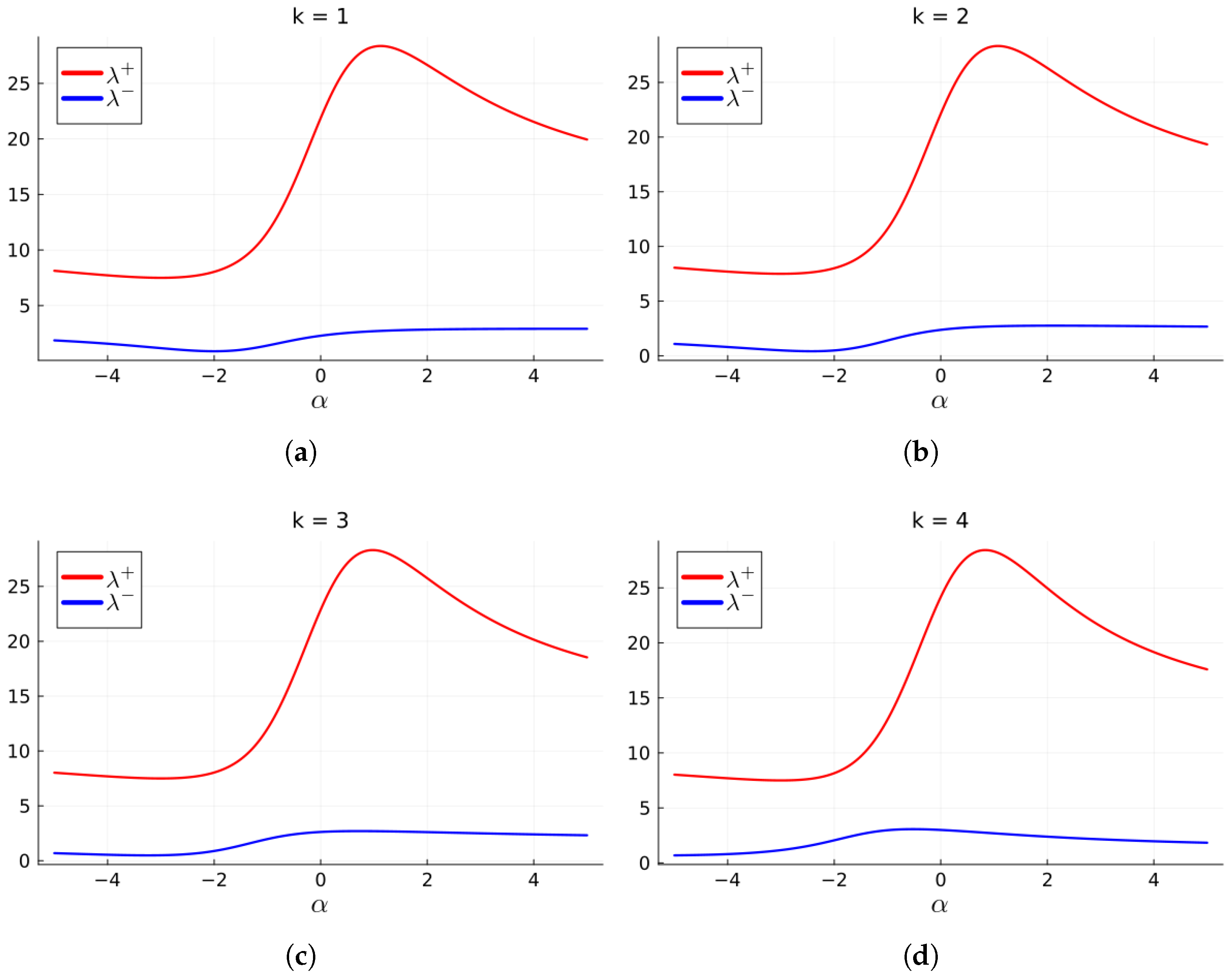
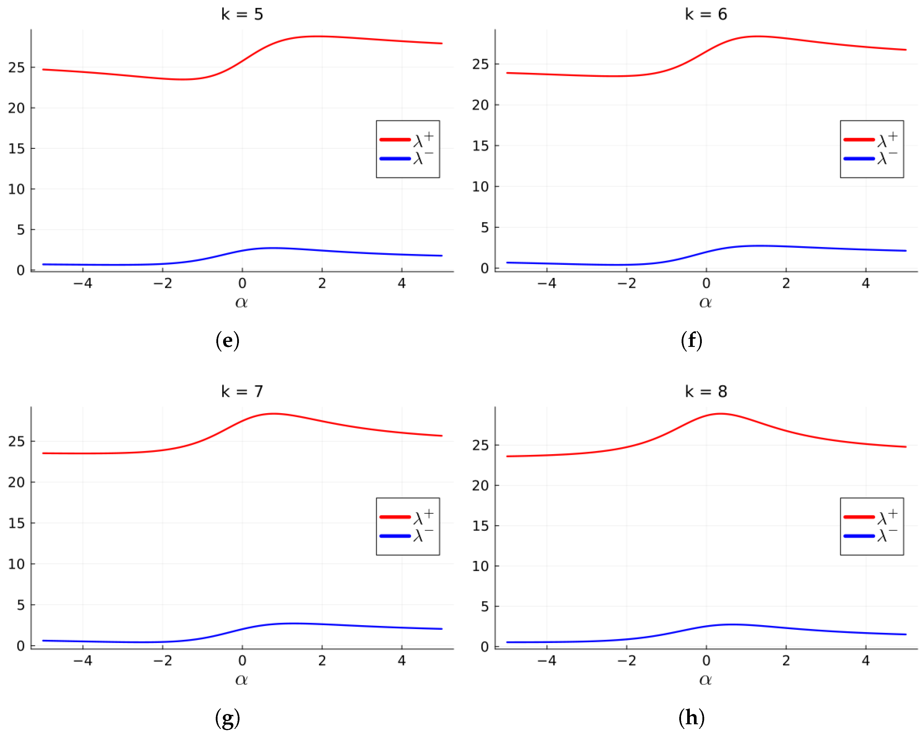
The solution for ${\lambda }^{-}$ and ${\lambda }^{+}$ using (26) and (31) is shown in

Table 1. Solution of Example 1.

k	${\mathit{\alpha }}_0,$${\tilde{\mathit{\alpha }}}_0$	$\mathit{\alpha }$	$\mathit{F}\left(\mathit{\alpha }\right),$$\tilde{\mathit{F}}\left(\mathit{\alpha }\right)$	${\mathit{\lambda }}^{-}$	${\mathit{\lambda }}^{+}$
1	0.826722	0.710321	1.86 × ${10}^{-09}$	2.614485	27.601089
2	0.826197	0.690819	−1.86 × ${10}^{-09}$	2.637621	27.642029
3	0.837001	0.644609	9.31 × ${10}^{-10}$	2.700265	27.756653
4	0.865323	0.570751	4.66 × ${10}^{-10}$	2.834633	28.043900
5	1.013646	0.555864	−3.49 × ${10}^{-10}$	2.691661	27.428588
6	0.910219	0.433913	−6.40 × ${10}^{-10}$	2.414374	27.600672
7	0.739681	0.296971	−2.04 × ${10}^{-10}$	2.328878	28.018525
8	0.473212	0.154739	−2.47 × ${10}^{-10}$	2.613206	28.807700

. From this, we can accept 2.328878 as an upper bound for ${\lambda }_1$ and 28.807700 as a lower bound for ${\lambda }_8$. These are acceptable given the relative ease of computation. In order to obtain a superior lower bound, we solve (33) for optimal $\alpha$ and substitute into (14). These results are summarized in

Table 2. Solution of Example 1 using (33).

k	${\mathit{\alpha }}_0$	$\mathit{\alpha }$	${\mathit{\lambda }}^{\prime -}\left(\mathit{\alpha }\right)$	${\mathit{\lambda }}^{-}$
1	−2.00	−1.998667	0.00 × ${10}^{0\phantom{-0}}$	0.888395
2	−2.00	−2.426749	−1.33 × ${10}^{-15}$	0.416356
3	−2.50	−3.242623	5.27 × ${10}^{-16}$	0.490469
4	−4.00	−5.982560	−5.55 × ${10}^{-17}$	0.668332
5	−3.00	−3.211123	0.00 × ${10}^{0\phantom{-0}}$	0.639657
6	−2.00	−2.256362	1.70 × ${10}^{-16}$	0.394002
7	−2.50	−2.527823	1.11 × ${10}^{-16}$	0.425852
8	−4.00	−5.068167	0.00 × ${10}^{0\phantom{-0}}$	0.543244

. Similarly, to obtain a superior upper bound, we solve (34) for optimal $\alpha$ and substitute into (14). The corresponding results are summarized in

Table 3. Solution of Example 1 using (34).

k	${\mathit{\alpha }}_0$	$\mathit{\alpha }$	${\mathit{\lambda }}^{\prime +}\left(\mathit{\alpha }\right)$	${\mathit{\lambda }}^{+}$
1	1.00	1.126413	9.16 × ${10}^{-16}$	28.368499
2	1.20	1.073185	6.25 × ${10}^{-16}$	28.328146
3	1.00	0.976169	−6.23 × ${10}^{-15}$	28.308683
4	0.75	0.835843	1.67 × ${10}^{-16}$	28.428059
5	1.50	1.884316	3.89 × ${10}^{-16}$	28.814222
6	1.00	1.290095	−6.07 × ${10}^{-16}$	28.378167
7	0.75	0.788489	−3.89 × ${10}^{-16}$	28.355043
8	0.00	0.356960	−1.67 × ${10}^{-16}$	28.882906

. From these, we obtain the lower bound 0.394002 and the upper bound 28.882906 However, the latter process requires a good enough starting value for $\alpha$ in the corresponding Newton routine, failing which there is divergence, a value of $\alpha$ that maximizes the lower bound, a value of $\alpha$ that minimizes the upper bound, or convergence to a complex zero. These starting values are obtained graphically for different values of k, as depicted in Figure 1. We shall thus not generate these results for further examples.

Example 2.

Here we consider the pentadiagonal matrix of odd order $n=11$ [17] given by

$$\begin{array}{c}\hfill \mathbf{A}=\left[\begin{array}{ccccccccccc}\hfill -1& \hfill 2& \hfill 1& \hfill & & \hfill & & \hfill & & \hfill & \\ \hfill 2& \hfill \phantom{-}0& \hfill 2& \hfill 1& \hfill & & \hfill & & \hfill & & \\ \hfill 1& \hfill 2& \hfill \phantom{-}0& \hfill 2& \hfill 1& \hfill & & \hfill & & \hfill & \\ \hfill & \hfill 1& \hfill 2& \hfill \phantom{-}0& \hfill 2& \hfill 1& \hfill & & \hfill & & \\ \hfill & \hfill & \hfill 1& \hfill 2& \hfill \phantom{-}0& \hfill 2& \hfill 1& \hfill & & \hfill & \\ \hfill & \hfill & & \hfill 1& \hfill 2& \hfill \phantom{-}0& \hfill 2& \hfill 1& \hfill & & \\ \hfill & \hfill & & \hfill & \hfill 1& \hfill 2& \hfill \phantom{-}0& \hfill 2& \hfill 1& \hfill & \\ \hfill & \hfill & & \hfill & & \hfill 1& \hfill 2& \hfill \phantom{-}0& \hfill 2& \hfill 1& \\ \hfill & \hfill & & \hfill & & \hfill & \hfill 1& \hfill 2& \hfill \phantom{-}0& \hfill 2& \hfill 1\\ \hfill & \hfill & & \hfill & & \hfill & & \hfill 1& \hfill 2& \hfill \phantom{-}0& \hfill 2\\ \hfill & \hfill & & \hfill & & \hfill & & \hfill & \hfill 1& \hfill 2& \hfill -1\end{array}\right],\end{array}$$

with

$$\begin{array}{cc}\hfill {\lambda }_1& =-3\hfill \\ \hfill {\lambda }_{11}& ={\left[1-2cos\left(\frac{11\pi }{12}\right)\right]}^2-3\hfill \\ \hfill & \approx 5.595754.\hfill \end{array}$$

For Example 2, we merely omit the last row and last column of the matrix to obtain and even-order submatrix. However, omission of the $p_{th}$ row and column will achieve a similar purpose, though with different results. From

Table 4. Solution for Example 2. Results for deletion of row and column 11.

k	${\mathit{\alpha }}_0,$${\tilde{\mathit{\alpha }}}_0$	$\mathit{\alpha }$	$\mathit{F}\left(\mathit{\alpha }\right),$$\tilde{\mathit{F}}\left(\mathit{\alpha }\right)$	${\mathit{\lambda }}^{-}$	${\mathit{\lambda }}^{+}$
1	1.000000	0.345487	1.82 × ${10}^{-12}$	3.497548	5.260788
2	0.902669	0.598199	0.00 × ${10}^{0\phantom{-0}}$	3.255361	5.041520
3	1.164888	0.708619	−7.28 × ${10}^{-12}$	3.262788	5.025014
4	1.050408	0.768007	−1.46 × ${10}^{-11}$	3.431253	5.038625
5	2.694508	1.265825	−2.91 × ${10}^{-11}$	3.291750	5.141396
6	−3.242201	−2.259370	−3.73 × ${10}^{-09}$	0.089968	4.378438
7	0.696487	0.800915	3.64 × ${10}^{-12}$	3.464532	5.046424
8	0.512421	0.786430	2.91 × ${10}^{-11}$	3.371885	5.036684
9	0.627825	0.659950	−7.28 × ${10}^{-12}$	3.347260	5.046034
10	1.073686	0.411161	3.64 × ${10}^{-12}$	3.431177	5.198358

, we accept 0.089968 as an upper bound for ${\lambda }_1$ and 5.260788 as a lower bound for ${\lambda }_{11}$. We additionally summarize in

Table 5. Solution for Example 2. Best bounds from deletion of row and column p.

p	${\mathit{\lambda }}^{-}$	${\mathit{\lambda }}^{+}$
1	−0.066734	5.262994
2	1.922344	4.956660
3	0.001084	4.818508
4	2.070744	4.818508
5	2.046900	4.601543
6	3.995904	4.515387
7	2.025074	4.602222
8	2.070744	4.816596
9	0.190265	4.816596
10	2.061973	4.946304
11	0.089968	5.260788

the best bounds obtained by deleting each of the other rows and corresponding columns. From Table 5, the best choices for extreme inner bounds are obviously −0.066734 and 5.262994 In

Table 6. Solution for Example 2. Best bounds from padding to even order.

p	${\mathit{\lambda }}^{-}$	${\mathit{\lambda }}^{+}$
0	2.620531	5.095542
1	2.620531	5.095542
2	2.620531	5.095542
3	2.620531	5.095542
4	2.620531	5.095542
5	2.626640	5.095542
6	−0.107061	5.095352
7	−0.107061	5.095406
8	−0.107061	5.095406
9	−0.107061	5.095406
10	−0.107061	5.095406
11	−0.107061	5.095406

, we summarize the effect of padding the matrix to even order. Several results are similar, since the padding position does not affect the spectrum of all such padded matrices. This is because each padded matrix is similar to the other by a permutation similarity transformation. From this table, −0.107061 and 5.095542 are acceptable bounds.

Example 3.

Here we consider the dense matrix $\mathbf{A}$ of order 9 given by $\mathbf{A}=\mathbf{R}\mathbf{D}\mathbf{R}$, where $\mathbf{R}=\mathbf{I}-2{\mathbf{ww}}^t$, $\mathbf{w}=\frac{1}{3}[1,1,\cdots ,1]$, and $\mathbf{D}$ is a chosen diagonal matrix. Since $\mathbf{R}$ is an involution, $\sigma \left(\mathbf{A}\right)=\sigma \left(\mathbf{D}\right)=\{-10,5,6,7,8,9,10,11,20\}$. The results using deletion are presented in

Table 7. Solution for Example 3. Best bounds from deletion of row and column p.

p	${\mathit{\lambda }}^{-}$	${\mathit{\lambda }}^{+}$
1	1.058718	10.592087
2	3.068791	11.066702
3	3.205324	11.194483
4	3.251441	11.345256
5	3.280746	11.517792
6	3.453696	11.541006
7	3.601736	11.588090
8	3.730502	11.680606
9	−5.823999	12.713623

. From this the best bounds are −5.823999 and 12.713623 Results using padding are presented in

Table 8. Solution for Example 3. Best bounds from padding to even order.

p	${\mathit{\lambda }}^{-}$	${\mathit{\lambda }}^{+}$
0	1.980210	11.600000
1	1.980210	11.600000
2	1.980210	11.600000
3	1.980210	11.600000
4	1.980210	11.600000
5	3.210315	12.506688
6	3.200135	12.506688
7	3.200043	12.506688
8	3.200003	12.506688
9	3.200486	12.506700

. Here the accepted bounds are 1.980210 and 12.506700 A similar pattern of results are obtained as for padding in Example 2. If padding is to be used, then it is only necessary to prepend or append the padding to the matrix.

Example 4.

Here we consider the Hilbert matrix $\mathbf{A}$ of order 10 given by

$$\begin{array}{c}\hfill a_{ij}=\frac{1}{i+j-1},i,j=1,2,\cdots ,10.\end{array}$$

This is a highly ill-conditioned matrix with ${\lambda }_1\approx 0$ and ${\lambda }_{10}=1.751920$.

The results are depicted in

Table 9. Solution for Example 4.

k	${\mathit{\alpha }}_0,$${\tilde{\mathit{\alpha }}}_0$	$\mathit{\alpha }$	$\mathit{F}\left(\mathit{\alpha }\right),$$\tilde{\mathit{F}}\left(\mathit{\alpha }\right)$	${\mathit{\lambda }}^{-}$	${\mathit{\lambda }}^{+}$
1	2.416906	1.122961	0.00 × ${10}^{0\phantom{-0}}$	0.114456	1.561871
2	0.812592	0.730081	−2.73 × ${10}^{-12}$	0.107768	1.488724
3	0.854452	0.563215	0.00 × ${10}^{0\phantom{-0}}$	0.113670	1.509045
4	0.902925	0.460570	−2.27 × ${10}^{-13}$	0.118454	1.537182
5	0.939411	0.389961	1.14 × ${10}^{-13}$	0.121675	1.563673
6	0.862024	0.392434	3.77 × ${10}^{-13}$	0.103398	1.490751
7	0.804749	0.338647	9.95 × ${10}^{-14}$	0.100977	1.495043
8	0.755895	0.301870	−2.13 × ${10}^{-13}$	0.099599	1.499771
9	0.713507	0.272798	−2.10 × ${10}^{-13}$	0.098871	1.504251
10	0.676250	0.248981	−3.48 × ${10}^{-13}$	0.098587	1.508395

. The minimum upper bound for ${\lambda }_1$ is accepted as 0.098587, while the maximum lower bound for ${\lambda }_{10}$ is given by 1.563673.

3. Conclusions

We have provided a rather inexpensive procedure to obtain optimal inner bounds for the extreme eigenvalues of real symmetric matrices. These bounds depend only on a single parameter and arise from approximation over a two-dimensional subspace of ${\mathbb{R}}^n$. They can be used to locate more accurately the spectrum of the matrix on $\mathbb{R}$. It is encouraged that others extend this idea of subspace approximation of eigenvalues to $r-$ invertible matrices over antirings [18].

References

1. Golub, G.; Uhlig, F. The QR algorithm: 50 years later–its genesis by John Francis and Vera Kublanovskaya, and subsequent developments. IMA J. Numer. Anal. 2009, 29, 467–485. [Google Scholar] [CrossRef]
2. Coulson, C.A.; Haskins, P.J. On the relative accuracies of eigenvalue bounds. J. Phys. B At. Mol. Phys. 1973, 6, 1741–1750. [Google Scholar] [CrossRef]
3. Kato, T. On the upper and lower bounds of eigenvalues. Phys. Rev. Lett. 1950, 77, 334–339. [Google Scholar] [CrossRef]
4. Ovtchinnikov, E.E. Lehmann bounds and eigenvalue error estimation. SIAM J. Numer. Anal. 2011, 49, 2078–2102. [Google Scholar] [CrossRef]
5. Delves, L.M. On the Temple lower bound for eigenvalues. J. Phys. A Gen. Phys. 1972, 5, 1123–1129. [Google Scholar] [CrossRef]
6. Brauer, A.; Mewbom, A.C. The greatest distance between two characteristic roots of a matrix. Duke Math. J. 1959, 26, 653–661. [Google Scholar] [CrossRef]
7. Horn, R.; Johnson, C.A. Matrix Analysis; Cambridge University Press: Cambridge, UK, 2012; pp. 345–346. [Google Scholar]
8. Brauer, A. Limits for the characteristic roots of a matrix: VII. Duke Math. J. 1958, 25, 583–590. [Google Scholar] [CrossRef]
9. Wolkowicz, H.; Styan, G.P.H. Bounds for eigenvalues using traces. Linear Algebra Appl. 1980, 29, 471–506. [Google Scholar] [CrossRef]
10. Sharma, R.; Kumar, R.; Saini, R. Note on Bounds for Eigenvalues using Traces. arXiv 2014, arXiv:1409.0096. [Google Scholar] [CrossRef]
11. Singh, P.; Singh, V.; Singh, S. New bounds for the maximal eigenvalues of positive definite matrices. Int. J. Appl. Math. 2022, 35, 685–691. [Google Scholar] [CrossRef]
12. Singh, P.; Singh, S.; Singh, V. Results on Bounds of the Spectrum of Positive Definite Matrices by Projections. Aust. J. Math. Anal. Appl.. 2023, 20, 1–10. [Google Scholar]
13. Singh, P.; Singh, S.; Singh, V. New Inner Bounds for the Extreme Eigenvalues of Real Symmetric Matrices. IAENG Int. J. Appl. Math. 2024, 54, 871–876. [Google Scholar]
14. Liao, W.; Long, P. Distribution of Eigenvalues and Upper Bounds of the Spread of Interval Matrices. Mathematics 2023, 11, 4032. [Google Scholar] [CrossRef]
15. Yuan, Q.; Yang, Z. A Fast Algorithm for the Eigenvalue Bounds of a Class of Symmetric Tridiagonal Interval Matrices. AppliedMath 2023, 3, 90–97. [Google Scholar] [CrossRef]
16. Hwang, S.G. Cauchy’s Interlace Theorem for Eigenvalues of Hermitian Matrices. Am. Math. Mon. 2004, 111, 157–1579. [Google Scholar] [CrossRef]
17. Gregory, R.T.; Karney, D.L. A Collection of Matrices for Testing Computational Algorithms; Robert, E., Ed.; Krieger Publishing Company: Huntington, WV, USA; New York, NY, USA, 1978; p. 57. [Google Scholar]
18. Wang, A.; Cheng, C.; Wang, L. On r-invertible matrices over antirings. Publ. Math. Debr. 2025, 106, 445–459. [Google Scholar] [CrossRef]
Figure 1. Variation in λ and λ + with α for example 1, for different positions k of α , from which starting values of α are chosen for Newton’s routine. (a) k = 1 , (b) k = 2 , (c) k = 3 , (d) k = 4 , (e) k = 5 , (f) k = 6 , (g) k = 7 , (h) k = 8 .
Symmetry 17 02031 g001aSymmetry 17 02031 g001b